
Multiple Sound Source Localization, Separation, and Reconstruction by Microphone Array: A DNN-Based Approach

1
College of Electronics and Information Engineering, Shenzhen University, Shenzhen 518060, China
2
Department of Mechanical Engineering, The Hong Kong Polytechnic University, Hung Hom, Kowloon 999077, Hong Kong
*
Author to whom correspondence should be addressed.
Appl. Sci. 2022, 12(7), 3428; https://doi.org/10.3390/app12073428
Submission received: 1 March 2022
/
Revised: 23 March 2022
/
Accepted: 27 March 2022
/
Published: 28 March 2022
(This article belongs to the Special Issue Machine Learning in Vibration and Acoustics)
Abstract
:Synchronistical localization, separation, and reconstruction for multiple sound sources are usually necessary in various situations, such as in conference rooms, living rooms, and supermarkets. To improve the intelligibility of speech signals, the application of deep neural networks (DNNs) has achieved considerable success in the area of time-domain signal separation and reconstruction. In this paper, we propose a hybrid microphone array signal processing approach for the nearfield scenario that combines the beamforming technique and DNN. Using this method, the challenge of identifying both the sound source location and content can be overcome. Moreover, the use of a sequenced virtual sound field reconstruction process enables the proposed approach to be quite suitable for a sound field which contains a dominant, stronger sound source and masked, weaker sound sources. Using this strategy, all traceable, mainly sound, sources can be discovered by loops in a given sound field. The operational duration and accuracy of localization are further improved by substituting the broadband weighted multiple signal classification (BW-MUSIC) method for the conventional delay-and-sum (DAS) beamforming algorithm. The effectiveness of the proposed method for localizing and reconstructing speech signals was validated by simulations and experiments with promising results. The localization results were accurate, while the similarity and correlation between the reconstructed and original signals was high.
1. Introduction
Deep learning-based sound source separation and reconstruction methods have significantly progressed in recent years [1,2]. Relevant speech signal state-of-the-art neural network technologies can be applied in various scenarios, such as speech enhancement and human–computer interactions [3,4,5,6]. As has been reported, the denoising performance of deep neural networks (DNNs) in signal processing areas is promising in low signal-to-noise ratios and reverberant environments [7,8]. However, in certain situations, for example, the active greetings of service robots in supermarkets and residences, accurate physical positions of the sound sources and accurate descriptions of the content of the acoustic signals are required. The spatial information of sound sources can also be useful for signal enhancement and other post-processing approaches. For the aforementioned and other potential scenarios, we propose a hybrid multichannel signal processing approach using a set of microphones for multiple sound source localization, separation, and reconstruction.
Over the past few decades, a variety of sound source separation and reconstruction methods have been developed for automatic speech recognition (ASR) systems. The multi-channel blind source separation (BSS) technique, which is based on independent component analysis (ICA), is one of the most widely used methods [9,10,11,12]. In a large number of ICA methods, the well-known fast-ICA is one of the most popular BSS techniques for separating and estimating non-Gaussian sound sources without any prior knowledge of the mixing process [10,13]. It is based on the optimization of a contrast function that measures the non-Gaussianity of the source. When the non-Gaussian nature of the modified signals is maximized, these modified signals are considered to be independent signals. As a result, the independent sources can be separated by iteratively modifying the mixed signals with a so-called unmixing matrix. The main advantage of the fast-ICA technique is its computational efficiency. These techniques have promising results for the separation of multiple independent sound sources. However, the locations of the sound sources cannot be determined directly after they are applied. The ASR system utilizes the artificial neural network (ANN) or DNN as a classification decoder to transcribe speech signals into words and text. Prior knowledge of speech signals, such as their acoustic features, and the pronunciation dictionary (PD) are required before processing [9]. Recently, the ASR system has been improved and developed to work with ego noise and to locate the sound source by binaural sound source localization (SSL) [14]. For the humanoid robot ASR system introduced in [14], the utilization of spatial information from binaural SSL could significantly improve the accuracy of speech recognition, even in a reverberant environment. As stated in [14], the spatial information decoded by microphones could be used to achieve multi-perception fusion between the auditory and visual senses of artificial intelligence (AI). However, except for the presence of prior knowledge, the other drawback of this method is that it requires a large number of sound sources.
An alternative to the aforementioned methods is the larger microphone array, which could provide a more accurate coordinate value in the scanning area instead of an incident angle [15]. Using a large microphone array, the acoustic imaging and signal processing approach, which contains near-field acoustical holography (NAH) and beamforming, has been widely applied in various industrial scenarios [16,17,18,19]. The NAH technique could map the sound field at every frequency of interest measured by the array. Therefore, a very precise sound source distribution can be provided because of the short-wave radiating distance between the microphone array plane and the sound source plane [18]. However, in many applications, a microphone array cannot be installed at such a short distance from the source plane. In addition, the area of the measured plane is limited to the dimension of the microphone array.
Various acoustic beamformers are regarded as the most suitable approaches for sound source localization in the far field, such as speech enhancement and human–computer interactions in indoor public areas. Beamforming techniques have been developed for decades [20,21]. In addition, an attempt to integrate neural networks (NNs) with acoustic beamformers has proved that NNs could work as front-end in ASR systems for practical SSL scenarios [22,23,24]. Every microphone channel signal of this neural mask-based beamformer is pre-processed through NNs directly, to achieve high recognition rates in far-field scenarios. With respect to acoustic beamformers, in the SSL area, most of the acoustic beamformers are operated in the frequency domain for more accurate localization performances and shorter processing durations, such as in the widely used, linearly constrained minimum variance (LCMV) method, the multiple signal classification (MUSIC) technique, and the well-known deconvolution methods, including the CLEAN algorithm and the deconvolution approach for the mapping of acoustic sources (DAMAS) algorithm [25,26,27,28,29,30]. However, to simultaneously acquire the signal features of sound sources in the time domain with their spatial information, the use of the conventional delay-and-sum (DAS) beamforming algorithm is regarded as a prerequisite so that the localization, separation, and reconstruction approaches of the multiple sound sources can be achieved concurrently [20]. The time-domain DAS beamforming algorithm utilizes a weighting function to compensate for the time delay in each measurement channel, and the compensated signals reinforce each other so that their summation can be maximized [31]. Wang et al. proved that a roughly estimated time series could be obtained at each scanning point with two sound sources in the scanning area, experimentally, by weighting different time delays and compensating for distance attenuations for each measurement channel [32]. Thus, after the location of the sound source is determined by calculating the maximum summation of the compensated signals on the scanning plane, a preliminary estimated signal of the dominant sound source can be obtained. Based on this, the main logic of the proposed signal processing approach is that, first, the location and rough time-domain features of the dominant sound source can be identified and characterized by a time-domain DAS beamformer. Then, the denoising approach is performed using supervised learning DNNs [33] so that the dominant sound source can be reconstructed. Subsequently, the signals from the dominant sound source are subtracted from the originally received signals, and the initial beamforming sound map is updated. Since the dominant sound source is localized and reconstructed, the received signals of all channels will be subtracted by this dominant source signal to perform the next iteration. By repeating this loop, multiple sound sources in the sound field can be localized and reconstructed. As the time consumption of time-domain DAS beamformer is extremely high, to achieve the real-time localization and separation performance, the computing speed could be improved by using a frequency-domain beamformer to estimate the initial location of the dominant sound source. Considering the broadband feature of the speech signal, a broadband weighted multiple signal classification (BW-MUSIC) method is used in this study to balance the selection of the computed frequency and computation time [34]. Moreover, to make full use of the feature information contained in the speech, four parameters are extracted from the pending signal: the mel-frequency cepstral coefficients (MFCC), amplitude modulation spectrum (AMS), gammatone filter bank power spectra (GFPS), and relative spectral transformed perceptual linear prediction coefficients (RASTA-PLP) [35,36]. A schematic of the proposed method is shown in Figure 1.
2. Methodologies
2.1. Sound Source Localization
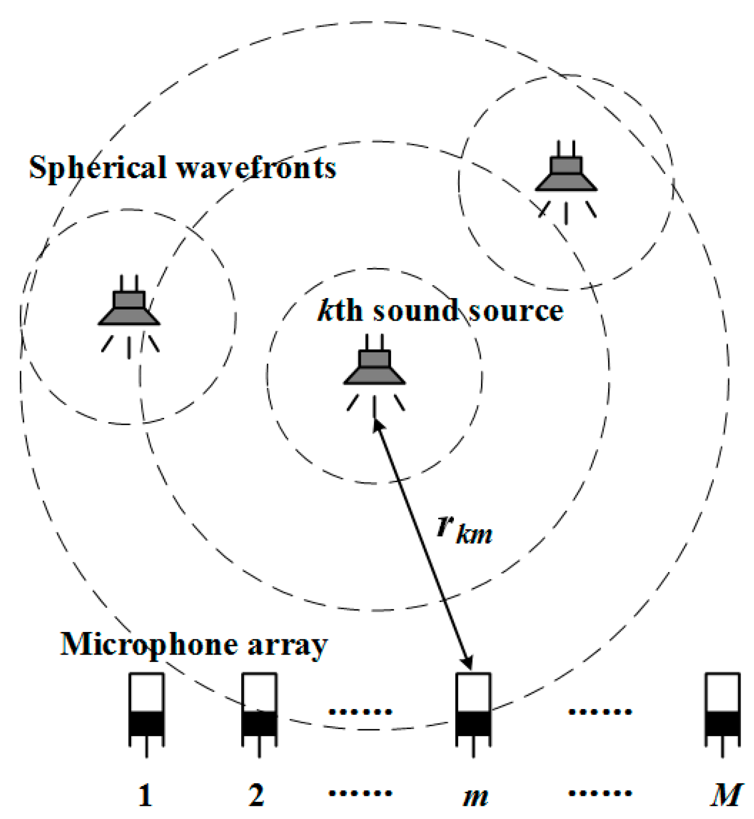
Unlike frequency-domain acoustic beamformers, which have undergone rapid development, few time-domain algorithms have been proposed in the past because of their high computational cost [37]. One of the most famous acoustic beamformers is the conventional DAS beamformer, which is considered effective and accurate for localizing moving, transient, and broadband sound sources based on various indicators, such as the peak value and root mean square (RMS) [20,38]. For an accurate localization performance, the spherical wave-front assumption of the sound wave propagation model is adopted so that the scanning region is meshed with certain horizontal and vertical coordinates.
Figure 2 illustrates the spherical wavefronts from N, point sound sources, incident on a linear array of M, microphones. The sound signals received at the mth () microphone can be expressed as
where , and the total sound signals received by the microphone array, can be expressed as
where is the signal from the kth sound source, is the incoherent noise, represents the sound pressure attenuation factor due to the distance between the sound source and microphone, represents the time delay, and is the speed of sound. With respect to a positional parameter , which is the distance between the scanning point and the mth microphone, an intentional compensating time delay is applied to each measured signal, and the traditional DAS beamformer output can be derived by summing and averaging all the delayed signals, i.e.,
and it is a function of time and space [20,37]. To indicate the spatial information of the dominant sound source in the scanning area only, an expectation operator, E, is applied such that the corresponding beamforming power can be expressed as
To achieve a higher accurate localization performance, the MUSIC algorithm uses the eigen-decomposition of the correlation matrix of the measured sound signal to extract the signal and noise subspaces. After the eigen-decomposition of the correlation matrix, it can be observed that the eigenvectors of the noise subspace are orthogonal to the basis vectors of the signal subspace. Furthermore, the MUSIC beamforming output can be calculated by the inverse of a designed scan vector, which belongs to the subspace obtained by multiplying the signal subspace by the correlation matrix of the noise subspace [20,27,34].
Considering the measured, complex sound field described in Equation (2) of a specific frequency bin, , (2) can be expressed as
and the measured correlation matrix is
where each element represents the correlation between two microphone signals. The correlation matrix can be expressed in an eigen-decomposition form:
Because the columns of are orthogonal, the correlation matrix can be separated into two parts:
where and represent the signal subspace corresponding to the largest eigenvalues of , and and represent the noise subspace [20]. Because is orthogonal to the basis vectors of the signal subspace, the beamforming power calculated from the correlation matrix consisting of these eigenvectors is minimal for a scan vector belonging to the signal subspace. The inverse of this beamforming power indicates that the source location has a maximum value when the scan vector belongs to the signal subspace:
Considering the different contributions of each frequency in the spectrum, a weighted broadband MUSIC output can be expressed as
where the narrowband MUSIC output is averaged and weighted by the different contributions in the spectrum for each frequency bin, f [34]. Therefore, the interference of the non-dominating frequency band can be eliminated during the computation of the beamforming maps.
2.2. Preliminary Signal Estimation
Because the location of the kth sound source can be indicated by (10)—in other words, is known—the estimated temporal characteristics of the kth source can be obtained by taking the average of all the weighted signals:
In (11), the weighted signal is amplified to compensate for the time delay and attenuation of the amplitude due to the travelling distance of the sound wave from the source to each microphone. By substituting (1) into (11), the temporal estimation of the kth source can be rewritten as
In (12), the estimated source signals are divided into two parts by simplification: the first part is the real source signal , while the second part could be considered the error function , which represents the difference between the real source signal and estimated signal:
In general, the right side of contains three parts: (1) the contribution of the sound sources that have been localized before the kth source, (2) the contribution of the sound sources that have not been localized after the kth source, and (3) the contribution of the incoherent noise from each measurement signal. First, compared with the real source signal, , a weighted averaging by the difference between and in the error function would suppress the amplitude of and in (12), which means that the amplitude of is much smaller than . Therefore, can be regarded as a rough estimate of . This acceptable hypothesis is the precondition of the following separation and reconstruction approach. Subsequently, in the first part of can be replaced by . The real source signal, , can be estimated using an iteration computation as:
The virtual received signals could be updated by newly estimated source signals. The iteration process stops if no additional sound source appears. Finally, all in the first part are obtained from the updated beamforming maps.
It is worth mentioning that the estimation of by is rather rough, with large errors in (12). However, the errors that cumulate after the iterative calculations could significantly affect the reconstruction signals when the number of sound sources is large. Therefore, DNN technology is introduced to eliminate errors and to acquire an acceptable estimation of in the next section.
2.3. Denoising the Deep Neural Network
To improve the estimation performance in (14), is processed before the subtraction for each iteration by the DNN [33]. The DNN contains four hidden layers without any dropout regularization and is pre-trained in an unsupervised manner, with each layer possessing 2048, 4096, 2048, and 512 hidden neural units. In the training stage, the adaptive gradient descent method is adopted as the optimization process, in which the learning rate decreases from 0.08 to 0.001 as the epoch increases, and the mean square error (MSE) is selected as the loss function to measure the error between the prediction of DNN and the training target. The sigmoid function is adopted as the activation function in each hidden layer. Moreover, to make full use of the feature information contained in the speech, four parameters are extracted from the pending signal: MFCC, AMS, GFPS, and RASTA-PLP [35,36]. To obtain the MFCC involving the envelope and detail of the frequency spectrum, each piece of raw data is divided into frames of 20 ms, with a 10 ms overlap. The Hamming window is applied to each frame, and the short-time Fourier transform (STFT) is utilized to obtain the power spectrum, which can be converted to 31-dimensional (31-D) MFCC by a log operation and discrete cosine transform (DCT) in the mel scale. To obtain AMS, the full-wave rectification and the decreased sample by a factor of 4 are applied to the speech signal, which is divided into frames of 32 ms, with a 10 ms frame shift. The Hamming window and a 256-point fast Fourier transform (FFT) are applied to each frame to obtain the power spectrum, which is converted to a 15-dimensional (15-D) feature by utilizing 15 triangular windows uniformly centered from 15.6 400 Hz. To obtain GFPS, a 64-channel gammatone filter bank is applied to the speech signal to obtain sub-band signals, and the energy spectrum is derived from the energy function to sub-band signals. It is noted that the RASTA-PLP is the spectral feature of the sound signals. Generally, it is a modified linear prediction cepstral coefficient to make the extracted power spectrum more suitable for the processing characteristics of the human ear [39]. To obtain RASTA-PLP, RASTA filtering is applied to PLP, which can minimize the differences among the dominant formant structures of different speakers. After converting the power spectrum of the signal to the bark scale, the log application and RASTA filter were then applied to the resulting spectrum. Finally, by expanding the filtered log spectrum with an exponential function and performing a linear prediction analysis, the 13-D RASTA-PLP can be derived. The characteristics of the pending signal were obtained from these four parameters using their sequential derivatives. Although the speech signal is usually regarded as a non-stationary signal, it has been reported that within a diminutive duration range, the speech signal can be regarded as a stationary signal owing to the motion inertia of the vocal organ [40]. In addition, to preserve the time-domain characteristics of the speech signal spectrum, in speech signal analysis, researchers usually adopt a 20–30 ms frame length during processing [35,41]. As a result, the original irregular signal could exhibit periodic properties without losing too much edge information.
The Free Surfing-Tech Chinese Mandarin Corpus dataset, which was recorded in a silent indoor environment by a cell phone, was adopted in the learning and training stage of DNNs. The dataset contained 855 different speakers with 120 short utterances for each speaker. A dataset of 700 speakers was randomly selected as the training set, while the remaining data were the testing set. A suitable training target significantly affects the performance of the network training. Therefore, in this study, the ideal ratio mask (IRM), which can be calculated using a 64-channel gammatone filter bank, was utilized as the training target:
where and are composed of randomly selected data pieces s1, s2, and s3 from the training set. and denote the energy of clean and background sounds, respectively, in a specific time-frequency unit, and is a tunable parameter that scales the IRM [35]. In this study, was set as 0.5 to achieve better quality objective data. The IRM is similar to an ideal Wiener filter [33,35]. The data with a dimension of 246, the number of frames, the mentioned four features, and their derivations were utilized as the input of the DNNs. Subsequently, the appropriate mapping from the frequency spectrum to the training target could be obtained by the DNNs. Finally, the estimated ratio mask from the network is applied to the frequency spectrum of the mixture speaker data to obtain the target speech frequency spectrum. Therefore, a clean signal can be obtained by an inverse fast Fourier transform (IFFT).
The denoising performance of the DNNs was first verified using MATLAB. A mixed signal with a signal-to-noise ratio (SNR) of 15 dB was processed by the trained DNN, as shown in Figure 3b. The original signal shown in Figure 3a was randomly selected from the ST-CMDS data testing set, while the interference noise was generated by mixing two other randomly selected signals beforehand. Figure 3c shows the estimated result after denoising processing, which indicates that the original signal was well retained.
3. Simulation Results
To verify the proposed signal-processing approach, numerical simulations were performed using MATLAB. As shown in Figure 4a, three point sound sources were located at (0.7 m, 1.4 m), (0.6 m, 0.4 m), and (1.2 m, 0.4 m), and an annular simulative array with eight receivers was adopted around the sources. The directivity pattern of the microphone array is shown in Figure 4b by assuming a single frequency point source signal in the geometric center of the scanning area.
The eight-channel measured mixed signal, which is shown in Figure 5, consists of three randomly selected signals from the ST-CMDS data testing set that do not contain any additional noise.
3.1. Traditional Time-Domain Beamforming
Figure 6 shows the simulated beamforming map obtained by the DAS beamformer using (4) before the first iteration. The hotspot in Figure 6 indicates the location of the dominant sound source, s1. Because the sound power level (SWL) of s1 was relatively higher than those of s2 and s3, the locations of the sound sources of s2 and s3 can barely be observed in Figure 6. Thus, the spatial information from the sound map and the preliminary estimation of s1 by time-domain DAS is regarded as an initial value, and it can be easily removed from the mixed signal by the proposed method. A virtual measurement signal is created such that the first dominant sound source, s1, does not exist.
Figure 7 shows the beamforming maps obtained after removing s1. To verify the effectiveness of the denoising DNNs, the performance of the DAS beamformer with and without the DNNs was determined through controlled experiments as well. The location of the dominant sound source, s2, in a virtual upgraded sound area is shown in Figure 7a,b. The effectiveness of adding the DNNs before removing s1 was not remarkable in this step.
To further separate the measured mixed signal, s1 and s2 were both removed by analogous processes, while Figure 8 shows the corresponding beamforming maps. In Figure 8a, which shows a beamforming map obtained without pre-processing by DNNs, the location of s3 cannot be identified successfully because of the interference caused by the error generated after removing s1 and s2 from the mixed signal. This problem was resolved by DNN pre-processing, as shown in Figure 8b, where the location of s3 in the virtual upgraded sound area can now be observed. The results of virtual sound area reconstruction and the corresponding source locations shown in Figure 7b and Figure 8b verify the effectiveness of DNN denoising.
3.2. Weighted Broadband MUSIC
As the high computation time burden of the time-domain DAS beamformer conflicts with the real-time localization and separation requirements, an alternative localization approach, the so-called BW-MUSIC method, was utilized to balance the broadband feature of the speech signal and the real-time operation performance. In the simulation cases, the sampling rate of the speech signals from the ST-CMDS data set was 16,000 Hz; therefore, the analysis frequency band was set to 50–8000 Hz, and the step length was 50 Hz for the BW-MUSIC method. The total processing duration for one sound source was 78.037 s, measured by MATLAB with an Intel i7-6700 central processing unit (CPU) and 44 GB of random access memory (RAM).
The improved localization results obtained with the BW-MUSIC method are shown in Figure 9, in which the locations of s1, s2, and s3 are denoted in the beamforming maps conspicuously by the virtual upgraded measurement sound signal. Compared with Figure 6, Figure 7b and Figure 8b of the DAS beamformer, the localization results of BW-MUSIC in Figure 9a–c are much more accurate, with minor main-lobe-to-side-lobe ratios (MSRs) and higher resolution. More specifically, owing to the error elimination by the weighting summation and averaging calculation in the BW-MUSIC method, the sound sources could be significantly identified by the main lobes, which are the distinct hotspots in all the three figures, while the areas of the hotspots are smaller.
3.3. Performance Evaluation of the Localization Results
Table 1 shows the errors in the absolute distance of localization for different simulation methods. A maximal error of 0.79 m occurs in the DAS beamforming map after removing s1 and s2 without DNNs. In accordance with the localization results shown in the figures, the DNN-based beamforming method provides a smaller error, and the localization results can be observed to be accurate.
It is worth mentioning that the virtual measurement signal could not be constructed perfectly in the time domain. This means that the residual error after removing the dominant sound source could still be comparable in the upgraded sound area. Therefore, the location of s1 can still be observed in Figure 9b,c. The same conclusion can be drawn from the signal reconstruction section.
As the interference in the beamforming maps is usually generated by two other sound sources instead of side-lobes, in this case, the common MSR may lead to an inaccurate evaluation to describe the localization performance. Therefore, a parameter called the main-to-second-lobe level (MSEL) was defined and utilized in this study:
where Lm is the height of the main lobe, and Ls is the height of the second lobe generated by other sources. Figure 10a shows the MSEL results of the three sources using different approaches. First, the MSEL of the beamforming maps of the third source obtained by DAS without DNNs is negative, which means that this method fails to locate the third sound source, as shown in Figure 8a. The DNNs could significantly improve the MSEL in the beamforming maps after removing s1 and s2. Second, the MSEL of the BW-MUSIC method is not always higher than that of the DAS method, even though the BW-MUSIC method could provide distinct beamforming maps.
The effective SNR ranges of the different approaches were evaluated by MSEL as well. Since no additional noise was added in this case, the decay rate between the two adjacent sound sources was utilized to describe the SNR. For example, assuming that the primary amplitudes of the three sound sources were A1, A2, and A3, the actual amplitudes of the three sound sources in the simulation would be set to A1, 0.8A2, and 0.64A3 when the decay rate is 80%. Figure 10b shows the MSEL results of the beamforming maps after removing s1 and s2, which vary with the decay rate. Apparently, the DAS without DNNs method could not locate the third sound source at all the SNR ranges, while the other two approaches failed when the decay rate was lower than 20%. According to the curves shown in Figure 10b, a decay rate higher than 40% could be a reasonably effective SNR range for the DAS with the DNNs method. For BW-MUSIC with DNNs, the criterion should be higher than 60%.
3.4. Signal Separation and Reconstruction
The DNN-processed signals were extracted and removed from the mixed signal simultaneously. The performance of the reconstruction and separation of the original signals is shown in Figure 11. Figure 11(1a) shows the original s1 from the ST-CMDS data testing set; Figure 11(1b) shows the reconstructed s1 using the proposed method; Figure 11(1c) shows the cross-correlation function between them. The same dispositions are adopted for s2 and s3 in Figure 11(2a–c,3a–c), respectively. It can be noticed that the signals s2 and s3 contain rare information in the 0–0.5 s range in Figure 11(2a,3a). However, s1 contains a large amount of information within the same range. Under such conditions, the three mixed signals were well separated and reconstructed. Only a few residual errors could be observed in the 0–0.5 s range in Figure 9(2b,3b). Additionally, the sharp peaks close to 1 in the cross-correlation functions shown in Figure 11(1c,2c,3c) indicate that the two corresponding signals are strongly coherent with each other, while no time shift can be found at the horizontal ordinate.
4. Experimental Study
Experimental validation was carried out in a semi-anechoic chamber of the Institute of Vibration, Shock, and Noise (IVSN) at the Shanghai Jiao Tong University (SJTU). The background noise level of the semi-anechoic chamber is 15.6 dB (A), and the cut-off frequency is 100 Hz. The floor of the semi-anechoic chamber is solid, which could act as a work surface for supporting heavy items. In the experiments, a 56-channel spiral array with 40 enabled microphones was placed 2.404 m in front of the measurement plane. Three Philips BT25 Bluetooth loudspeakers were arranged in the measurement plane as sound sources. The acoustic signals were captured by Brüel & Kjær 4944-A microphones, which were calibrated by a Brüel & Kjær 4231 94 dB sound pressure calibration before the measurements. The sound pressure analog signals were converted into digital signals using a 42-channel Mueller-BBM MKII sound measurement system, and the sampling rate was 16,000 Hz. A snapshot of the experimental setup is presented in Figure 12.
As shown in Figure 12, the geometrical center of the spiral array, which was at a height of 1.39 m from the floor in the experiments, was set as the coordinate origin. Three sound sources, which were 1.752 m, 1.128 m, and 1.419 m from the floor, were supported by tripods. A laser level and the band tapes with a 0.001 m accuracy were utilized to measure the sound source locations. Accordingly, considering the length of the microphones, the coordinates of the three sound sources were (−0.800, 0.029, and 2.304 m), (0.007 m, −0.262 m, and 2.304 m), and (0.793 m, 0.362 m, and 2.304 m) in a near-field Cartesian coordinate system. The plane of the microphones was set as the x–z coordinate plane. Three randomly selected data pieces from the ST-CMDS data testing set were broadcast by loudspeakers on an endless loop in the measurements. A 40-channel mixed signal is shown in Figure 13.
The beamforming maps of the localization results obtained by the proposed process are shown in Figure 14. By adopting the BW-MUSIC method and denoising DNNs, the localization performance was found to be acceptable with obvious main lobes, which indicate the location of the sound source. The side lobes could barely be noticed in all the three figures. However, the area of the hotspots was larger than in the simulation results. As the experimental chamber is semi-anechoic, the lower resolution in Figure 14, compared to Figure 9, can be attributed to the ground reflection of sound waves. Table 2 shows the corresponding errors in the absolute distance of localization by BW-MUSIC. It is indicated that the three sound sources are localized accurately, with a location error of less than 0.15 m.
A comparison of the original signals from the dataset and the signals reconstructed by the proposed method is shown in Figure 15. The reconstructed signals shown in Figure 15(1b–3b) prove that the proposed method can successfully separate the three sound sources from the mixed measurement signal. However, the apparent discrepancy between the original and reconstructed signals indicates a worse performance of the signal reconstruction in the experimental study compared with the simulation results. As background noise is generated from the sound measurement system and the ground reflection interference of sound waves, in future work, a more robust denoising DNN for a lower SNR will be explored to improve the reconstruction performance.
5. Conclusions
The aim of this paper is to present a conceivable approach for real-time, multiple sound source, synchronistical localization, separation, and reconstruction. Its performance regarding the processing of speech signals from the ST-CMDS dataset was investigated through simulations and experiments. The major conclusions of this study are as follows.
1. By adopting the beamforming technique and denoising DNNs by numerical simulations and experimental studies, it is feasible to localize and separate the mixed multiple sound sources of speech signals in the time domain. The sound map of a DAS beamformer is formed by the superposition of the contributions of all sources in the sound field. Sources with lower SWLs may be masked by other sound sources with higher SWLs. Accordingly, compared with the traditional beamforming methods for multiple sound source localization, the proposed approach is quite suitable for a sound field containing a dominant sound source with masked weak sound sources, owing to the signal removal and virtual sound field reconstruction iteration. A decay rate higher than 60% could be an effective SNR range for the proposed method.
2. The time-domain signals were estimated and denoised using the DAS beamformer with DNNs. However, in reality, the computational cost of the time-domain DAS beamformer is unsuitable for potential applications. Thus, the localization procedure in the proposed approach is improved by the BW-MUSIC method, which is more flexible for broadband speech signals with an adjustable operational speed in the frequency domain. In particular, the accuracy and resolution of the sound source locations are enhanced by the BW-MUSIC method. The sound sources are localized accurately with a location error less than 0.001 m in the numerical simulations, and 0.15 m in the experimental study. The temporal characteristics of the source signals are well-extracted from the measurement signals during simulations, yet the signal reconstruction performance in the experiments is worse because of the ground reflection of sound waves and background noise.
3. The proposed approach could provide a potential criterion for determining whether a small hotspot in a beamforming map is the main lobe of a weaker source or the side lobe of a stronger source at another place, as each main sound source could be plotted on the beamforming map separately by iterations. This can be regarded as an alternative approach for source number estimation in a given sound field.
Author Contributions
L.C.: methodology, software, validation, formal analysis, data curation, and writing—original draft. G.C.: investigation, data curation, formal analysis, and writing—original draft. W.S.: supervision, conceptualization, and writing—review and editing. L.H.: funding acquisition, resources, and writing—review and editing. Y.-S.C.: writing—review and editing. All authors have read and agreed to the published version of the manuscript.
Funding
This work was supported, in part, by the National Natural Science Foundation of China (NSFC) under Grants 62101335, U1713217, and 61925108; in part by the Natural Science Foundation of Guangdong under Grant 2021A1515011706, and in part by the Foundation of Shenzhen under Grant JCYJ20190808122005605.
Institutional Review Board Statement
Not applicable.
Informed Consent Statement
Not applicable.
Data Availability Statement
Not applicable.
Acknowledgments
The authors would like to acknowledge the experimental support from Weikang Jiang and Liang Yu of SJTU.
Conflicts of Interest
The authors declare no conflict of interest.
References
- Qian, K.; Zhang, Y.; Chang, S.; Yang, X.; Florencio, D.; Hasegawa-Johnson, M. Deep learning based speech beamforming. In Proceedings of the 2018 IEEE International Conference on Acoustics, Speech and Signal Processing (ICASSP), Calgary, AB, Canada, 15–20 April 2018; pp. 5389–5393. [Google Scholar]
- Zhang, Z.; Xu, Y.; Yu, M.; Zhang, S.-X.; Chen, L.; Yu, D. ADL-MVDR: All deep learning MVDR beamformer for target speech separation. arXiv 2020, arXiv:2008.06994. [Google Scholar]
- Li, H.; Zhang, X.; Gao, G. Beamformed Feature for Learning-based Dual-channel Speech Separation. In Proceedings of the ICASSP 2020—2020 IEEE International Conference on Acoustics, Speech and Signal Processing (ICASSP), Barcelona, Spain, 4–8 May 2020; pp. 4722–4726. [Google Scholar]
- Qi, J.; Du, J.; Siniscalchi, S.M.; Ma, X.; Lee, C.-H. Analyzing Upper Bounds on Mean Absolute Errors for Deep Neural Network Based Vector-to-Vector Regression. IEEE Trans. Signal Process. 2020, 68, 3411–3422. [Google Scholar] [CrossRef]
- Qi, J.; Du, J.; Siniscalchi, S.M.; Ma, X.; Lee, C.-H. On mean absolute error for deep neural network based vector-to-vector regression. IEEE Signal Process. Lett. 2020, 27, 1485–1489. [Google Scholar] [CrossRef]
- Akhtiamov, O.; Sidorov, M.; Karpov, A.A.; Minker, W. Speech and Text Analysis for Multimodal Addressee Detection in Human-Human-Computer Interaction. In Proceedings of the Interspeech 2017, Stockholm, Sweden, 20–24 August 2017; pp. 2521–2525. [Google Scholar]
- Zhang, X.; Wang, D. Deep Learning Based Binaural Speech Separation in Reverberant Environments. IEEE/ACM Trans. Audio Speech Lang. Process. 2017, 25, 1075–1084. [Google Scholar] [CrossRef] [PubMed]
- Williamson, D.S.; Wang, D. Time-Frequency Masking in the Complex Domain for Speech Dereverberation and Denoising. IEEE/ACM Trans. Audio Speech Lang. Process. 2017, 25, 1492–1501. [Google Scholar] [CrossRef] [PubMed]
- Nasereddin, H.H.; Omari, A.A.R. Classification techniques for automatic speech recognition (ASR) algorithms used with real time speech translation. In Proceedings of the 2017 Computing Conference, London, UK, 18–20 July 2017; pp. 200–207. [Google Scholar]
- Hesse, C.W.; James, C.J. The FastICA algorithm with spatial constraints. IEEE Signal Process. Lett. 2005, 12, 792–795. [Google Scholar] [CrossRef]
- Saruwatari, H.; Kawamura, T.; Shikano, K. Blind source separation for speech based on fast-convergence algorithm with ICA and beamforming. In Proceedings of the 7th European Conference on Speech Communication and Technology, Aalborg, Denmark, 3–7 September 2001. [Google Scholar]
- Brems, D.J.; Schoeffler, M.S. Automatic Speech Recognition (ASR) Processing Using Confidence Measures. U.S. Patent 5,566,272, 15 October 1996. [Google Scholar]
- He, X.; He, F.; He, A. Super-Gaussian BSS Using Fast-ICA with Chebyshev–Pade Approximant. Circuits Syst. Signal Process. 2017, 37, 305–341. [Google Scholar] [CrossRef]
- Davila-Chacon, J.; Liu, J.; Wermter, S. Enhanced Robot Speech Recognition Using Biomimetic Binaural Sound Source Localization. IEEE Trans. Neural. Netw. Learn. Syst. 2019, 30, 138–150. [Google Scholar] [CrossRef] [Green Version]
- Benesty, J.; Chen, J.; Huang, Y. Microphone Array Signal Processing; Springer Science & Business Media: Berlin/Heidelberg, Germany, 2008. [Google Scholar]
- Chen, L.; Choy, Y.S.; Wang, T.G.; Chiang, Y.K. Fault detection of wheel in wheel/rail system using kurtosis beamforming method. Struct. Health Monit. 2019, 19, 495–509. [Google Scholar] [CrossRef]
- Yu, L.; Antoni, J.; Wu, H.; Jiang, W. Reconstruction of cyclostationary sound source based on a back-propagating cyclic wiener filter. J. Sound Vib. 2019, 442, 787–799. [Google Scholar] [CrossRef]
- Wu, H.; Jiang, W.; Zhang, H. A mapping relationship based near-field acoustic holography with spherical fundamental solutions for Helmholtz equation. J. Sound Vib. 2016, 373, 66–88. [Google Scholar] [CrossRef]
- Khan, S.; Huh, J.; Ye, J.C. Adaptive and Compressive Beamforming Using Deep Learning for Medical Ultrasound. IEEE Trans. Ultrason. Ferroelectr. Freq. Control. 2020, 67, 1558–1572. [Google Scholar] [CrossRef] [Green Version]
- Kim, Y.-H.; Choi, J.-W. Sound Visualization and Manipulation; John Wiley & Sons: Hoboken, NJ, USA, 2013. [Google Scholar]
- Chiariotti, P.; Martarelli, M.; Castellini, P. Acoustic beamforming for noise source localization—Reviews, methodology and applications. Mech. Syst. Signal Process. 2019, 120, 422–448. [Google Scholar] [CrossRef]
- Boeddeker, C.; Erdogan, H.; Yoshioka, T.; Haeb-Umbach, R. Exploring practical aspects of neural mask-based beamforming for far-field speech recognition. In Proceedings of the 2018 IEEE International Conference on Acoustics, Speech and Signal Processing (ICASSP), Calgary, AB, Canada, 15–20 April 2018; pp. 6697–6701. [Google Scholar]
- Masuyama, Y.; Togami, M.; Komatsu, T. Multichannel loss function for supervised speech source separation by mask-based beamforming. arXiv 2019, arXiv:1907.04984. [Google Scholar]
- Drude, L.; Heymann, J.; Haeb-Umbach, R. Unsupervised training of neural mask-based beamforming. arXiv 2019, arXiv:1904.01578. [Google Scholar]
- Jian, L.; Stoica, P.; Zhisong, W. On robust capon beamforming and diagonal loading. IEEE Trans. Signal Process. 2014, 51, 1702–1715, 2003. [Google Scholar]
- Chu, Z.; Yang, Y. Comparison of deconvolution methods for the visualization of acoustic sources based on cross-spectral imaging function beamforming. Mech. Syst. Signal Process. 2014, 48, 404–422. [Google Scholar] [CrossRef]
- Schmidt, R. Multiple emitter location and signal parameter estimation. IEEE Trans. Antennas Propag. 1986, 34, 276–280. [Google Scholar] [CrossRef] [Green Version]
- Sijtsma, P.; Merino-Martinez, R.; Malgoezar, A.M.N.; Snellen, M. High-resolution CLEAN-SC: Theory and experimental validation. Int. J. Aeroacoust. 2017, 16, 274–298. [Google Scholar] [CrossRef] [Green Version]
- Dougherty, R.P. Functional beamforming for aeroacoustic source distributions. In Proceedings of the 20th AIAA/CEAS Aeroacoustics Conference, Atlanta, GA, USA, 16–20 June 2014; p. 3066. [Google Scholar]
- Brooks, T.F.; Humphreys, W.M. A deconvolution approach for the mapping of acoustic sources (DAMAS) determined from phased microphone arrays. J. Sound Vib. 2006, 294, 856–879. [Google Scholar] [CrossRef] [Green Version]
- Byrne, D.; Craddock, I.J. Time-Domain Wideband Adaptive Beamforming for Radar Breast Imaging. IEEE Trans. Antennas Propag. 2015, 63, 1725–1735. [Google Scholar] [CrossRef]
- Wang, T.; Choy, Y. An approach for sound sources localization and characterization using array of microphones. In Proceedings of the 2015 International Conference on Noise and Fluctuations (ICNF), Xi’an, China, 2–6 June 2015; pp. 1–4. [Google Scholar]
- Wang, Y.; Wang, D. A deep neural network for time-domain signal reconstruction. In Proceedings of the 2015 IEEE International Conference on Acoustics, Speech and Signal Processing (ICASSP), South Brisbane, Australia, 19–24 April 2015; pp. 4390–4394. [Google Scholar]
- Chen, L.; Choy, Y.-S.; Tam, K.-C.; Fei, C.-W. Hybrid microphone array signal processing approach for faulty wheel identification and ground impedance estimation in wheel/rail system. Appl. Acoust. 2021, 172, 107633. [Google Scholar] [CrossRef]
- Wang, Y.; Narayanan, A.; Wang, D. On training targets for supervised speech separation. IEEE/ACM Trans. Audio Speech Lang. Process. 2014, 22, 1849–1858. [Google Scholar] [CrossRef] [PubMed] [Green Version]
- Yuxuan, W.; DeLiang, W. Towards Scaling Up Classification-Based Speech Separation. IEEE/ACM Trans. Audio Speech Lang. Process. 2013, 21, 1381–1390. [Google Scholar] [CrossRef] [Green Version]
- Dougherty, R. Advanced time-domain beamforming techniques. In Proceedings of the 10th AIAA/CEAS Aeroacoustics Conference, Manchester, UK, 10–12 May 2004; p. 2955. [Google Scholar]
- Seo, D.-H.; Choi, J.-W.; Kim, Y.-H. Impulsive sound source localization using peak and RMS estimation of the time-domain beamformer output. Mech. Syst. Signal Process. 2014, 49, 95–105. [Google Scholar] [CrossRef]
- Zulkifly, M.A.A.; Yahya, N. Relative spectral-perceptual linear prediction (RASTA-PLP) speech signals analysis using singular value decomposition (SVD). In Proceedings of the 2017 IEEE 3rd International Symposium in Robotics and Manufacturing Automation (ROMA), Kuala Lumpur, Malaysia, 19–21 September 2017; pp. 1–5. [Google Scholar]
- Rabiner, L.; Schafer, R. Theory and Applications of Digital Speech Processing; Prentice Hall Press: Hoboken, NJ, USA, 2010. [Google Scholar]
- Chen, J.; Wang, Y.; Wang, D. A feature study for classification-based speech separation at low signal-to-noise ratios. IEEE/ACM Trans. Audio Speech Lang. Process. 2014, 22, 1993–2002. [Google Scholar] [CrossRef]
Figure 1.
Schematic of the proposed method.

Figure 2.
Spherical wave-front model.

Figure 3.
Signal denoised by DNNs. (a) Original signal; (b) mixed signal; (c) estimated signal.

Figure 4.
Geometry of the simulation performed in MATLAB (a) and the directivity pattern of microphone array (b).
Figure 4.
Geometry of the simulation performed in MATLAB (a) and the directivity pattern of microphone array (b).

Figure 5.
Eight-channel measured mixed signal in the simulative study.

Figure 6.
Preliminary beamforming map by DAS.

Figure 7.
DAS Beamforming maps after removing s1. (a) Without DNNs; (b) with DNNs.

Figure 8.
DAS Beamforming maps after removing s1 and s2. (a) Without DNNs; (b) with DNNs.

Figure 9.
Beamforming maps obtained with the BW-MUSIC with DNNs. (a) s1; (b) s2; (c) s3.

Figure 10.
MSEL results of the three sources (a) and the effective SNR ranges (b).

Figure 11.
Original signals (a), reconstructed signals (b), and the cross-correlation function (c) between them: (1) s1, (2) s2, and (3) s3.
Figure 11.
Original signals (a), reconstructed signals (b), and the cross-correlation function (c) between them: (1) s1, (2) s2, and (3) s3.

Figure 12.
Experimental setup: three loudspeakers and the spiral microphone array in a semi-anechoic chamber.
Figure 12.
Experimental setup: three loudspeakers and the spiral microphone array in a semi-anechoic chamber.

Figure 13.
Forty-channel measured mixed signal in the experimental study.

Figure 14.
Localization results of the experimental study performed with BW-MUSIC and DNNs: (a) s1, (b) s2, and (c) s3.
Figure 14.
Localization results of the experimental study performed with BW-MUSIC and DNNs: (a) s1, (b) s2, and (c) s3.

Figure 15.
Original signals (a) and the reconstructed signals (b) in the experimental study: (1) s1, (2) s2, and (3) s3.
Figure 15.
Original signals (a) and the reconstructed signals (b) in the experimental study: (1) s1, (2) s2, and (3) s3.


Table 1.
Localization errors of the simulations.
| Sound Source | Localization Method | Error (m) |
|---|---|---|
| s1 | DAS | 0 |
| BW-MUSIC | 0 | |
| s2 | DAS without DNNs | 0.01 |
| DAS with DNNs | 0 | |
| BW-MUSIC with DNNs | 0 | |
| s3 | DAS without DNNs | 0.79 |
| DAS with DNNs | 0 | |
| BW-MUSIC with DNNs | 0 |
Table 2.
Localization error of the experimental study performed with BW-MUSIC and DNNs.
| Sound Source | Error (m) |
|---|---|
| s1 | 0.14 |
| s2 | 0.11 |
| s3 | 0.09 |
Publisher’s Note: MDPI stays neutral with regard to jurisdictional claims in published maps and institutional affiliations. |
© 2022 by the authors. Licensee MDPI, Basel, Switzerland. This article is an open access article distributed under the terms and conditions of the Creative Commons Attribution (CC BY) license (https://creativecommons.org/licenses/by/4.0/).
Share and Cite
MDPI and ACS Style
Chen, L.; Chen, G.; Huang, L.; Choy, Y.-S.; Sun, W. Multiple Sound Source Localization, Separation, and Reconstruction by Microphone Array: A DNN-Based Approach. Appl. Sci. 2022, 12, 3428. https://doi.org/10.3390/app12073428
AMA Style
Chen L, Chen G, Huang L, Choy Y-S, Sun W. Multiple Sound Source Localization, Separation, and Reconstruction by Microphone Array: A DNN-Based Approach. Applied Sciences. 2022; 12(7):3428. https://doi.org/10.3390/app12073428
Chicago/Turabian StyleChen, Long, Guitong Chen, Lei Huang, Yat-Sze Choy, and Weize Sun. 2022. "Multiple Sound Source Localization, Separation, and Reconstruction by Microphone Array: A DNN-Based Approach" Applied Sciences 12, no. 7: 3428. https://doi.org/10.3390/app12073428
Note that from the first issue of 2016, this journal uses article numbers instead of page numbers. See further details here.