Boundaries of Oscillatory Motion in Structures with Nonviscous Dampers

Abstract

In this paper, a new methodology for the determination of the boundaries between oscillatory and non-oscillatory motion for nonviscously damped nonproportional systems is proposed. It is assumed that the damping forces are expressed as convolution integrals of the velocities via hereditary exponential kernels. Oscillatory motion is directly related to the complex nature of eigensolutions in a frequency domain and, in turn, on the value of the damping parameters. New theoretical results are derived on critical eigenmodes for viscoelastic systems with multiple degrees of freedom, with no restrictions on the number of hereditary kernels. Furthermore, these outcomes enable the construction of a numerical approach to draw the critical curves as solutions of certain parameter-dependent eigenvalue problems. The method is illustrated and validated through two numerical examples, covering discrete and continuous systems.

1. Introduction

Currently, there are many applications, from micro-scale systems to large structures, that require the control of vibration, sound, and wave propagation for proper operation. New techniques to optimize energy dissipation have been proposed in recent years, from the consolidation of time-dependent viscoelastic materials [1,2,3,4], to the emergent phenomenon of metadamping [5,6]. In part, the advances in new dissipation mechanisms have been carried out thanks to the constant increase in computing capacity, since the new discoveries are generally accompanied by more complex mathematical models. In the context of vibration control with nonviscously damped materials, it is especially important to know how to choose the characteristics of the dissipative devices or materials to ensure that the system becomes overcritically damped in one or more modes. In this article, we investigate criticality in nonviscously damped multiple-degrees-of-freedom (dof) systems, considering any number of exponential hereditary kernels.

Nonviscous damping is characterized by dissipative forces which depend on the past history of the velocity response via convolution integrals over hereditary kernel functions. Denoting, with $\mathfrak{u}\left(t\right)\in {\mathbb{R}}^n$, the array with degrees of freedom, the equations of motion are expressed in integro-differential form, as [1]:

$$\mathbf{M}\ddot{\mathfrak{u}}+{\int }_{-\infty }^t\mathcal{G}(t-\tau )\dot{\mathfrak{u}}\mathrm{d}\tau +\mathbf{K}\mathfrak{u}=\mathfrak{f}\left(t\right),$$

(1)

where $\mathbf{M},\mathbf{K}\in {\mathbb{R}}^{n\times n}$ are the mass and stiffness matrices assumed to be positive definite and positive semidefinite, respectively; $\mathcal{G}\left(t\right)\in {\mathbb{R}}^{n\times n}$ represents the time-domain damping matrix, assumed to be symmetric. Viscous damping arises just as a particular form of Equation (1), with $\mathcal{G}\left(t\right)\equiv \mathbf{C}\delta \left(t\right)$, where $\mathbf{C}$ is the viscous damping matrix and $\delta \left(t\right)$ the Dirac’s delta function. Checking for solutions of the form $\mathfrak{u}\left(t\right)=\mathit{u}{e}^{st}$ in Equation (1) transforms the time-domain equations into a nonlinear eigenvalue problem with the form:

$$\left[s^2\mathbf{M}+s\mathbf{G}\left(s\right)+\mathbf{K}\right]\mathit{u}\equiv \mathbf{D}\left(s\right)\mathit{u}=\mathbf{0},$$

(2)

where $\mathbf{G}\left(s\right)=\mathcal{L}\left\{\mathcal{G}\left(t\right)\right\}\in {\mathbb{C}}^{n\times n}$ is the frequency-domain damping matrix, $\mathbf{D}\left(s\right)$ is the dynamical stiffness matrix, and $s=i\omega$ is the Laplace parameter. The roots of the characteristic equation:

$$det\left[\mathbf{D}\left(s\right)\right]=0,$$

(3)

are the eigenvalues of Equation (2). Viscoelastically damped structures are characterized as a frequency-dependent damping matrix. The time-domain response will be affected by the nature of the eigenvalues of Equation (2). In turn, complex eigenvalues are associated to oscillatory motion; meanwhile, real negative eigenvalues lead to nonoscillatory modes. When the nonviscous damping model is based on hereditary exponential kernels, something that will be assumed in the current investigation, the number of eigenvalues will be invariably greater than $2n$ because there exist p real nonviscous modes associated to hereditary exponential kernels [7,8]. Thus, undamped or lightly damped systems present $2n$ oscillatory modes with a relatively small real part in magnitude, together with p real nonviscous eigenvalues. However, as the damping level increases, the complex eigenvalues move away from the undamped ones in the complex plane. For high-damping forces, some conjugate–complex pair of eigenvalues may drop into the real axis, vanishing the oscillatory nature. The root locus in the complex plane depends on the damping parameters presented in the matrix $\mathbf{G}\left(s\right)$. In general, viscoelastic models are mathematically defined by several parameters so that the set of all of them defines a multidimensional parametric domain. The nature of eigenvalues closely depends on where the multidimensional point of such parameters lies. Critical manifolds are sets in this parametric domain, limiting the undercritically and overcritically damped regions. Geometrically, one-dimensional manifolds represent critical curves, which depicts critical relationships between two parameters. Then, critical regions are 2D areas enclosed by such critical curves. Lázaro [9] proved that critical manifolds of dynamical systems with viscoelastic damping can be found by eliminating the Laplace parameter s from the two equations:

$$det\left[\mathbf{D}\left(s\right)\right]=0,\frac{\partial }{\partial s}det\left[\mathbf{D}\left(s\right)\right]=0.$$

(4)

Purely viscous forces are characterized by being proportional to the velocity of the response. In the frequency domain, this fact simplifies the study of the critical damping conditions with respect to the use of nonviscous damping. In fact, Papargyri-Beskou and Beskos [10] proved that, for viscous systems, approximations of critical curves may be derived by assuming that the critical eigenvalues are $s=-{\omega }_j,1\le j\le n$, where ${\omega }_j$ denotes the jth natural undamped frequency. Bulatovic [11] proved new necessary and sufficient conditions for critical damping based on the determinant of the system and on the minors of certain matrices, depending on the eigenvalues. Mathematically, the inclusion of hereditary exponential kernels in the damping model leads to an increase of the order of the characteristic polynomial. The first attempts to determine the conditions of overcritical damping were proposed by Muravyov and Hutton [12] and Adhikari [13]. These works were developed with just one hereditary kernel, addressing the problem by carrying out an exhaustive analysis of the nature of the root of the resulting third-order characteristic polynomial. Müller [14] studied the nature of eigenvalues for single-dof systems based on a Zener three-parameter damping model. The critical oscillatory motion of nonviscous beams has been studied by Pierro [15], solving the eigenvalues for one and two exponential kernels and discussing their nature (real or complex). Wang [16] obtained fractional orders compatible with critical damping in fractional derivative-based, viscoelastic, classically damped structures. The problem of determining the critical manifolds of a single degree-of-freedom oscillator for any number of hereditary kernels has been analytically solved in exact form by Lázaro [17], by transforming Equation (4) into parametric closed-form expressions. For large multiple-dof systems, the general method proposed by Lázaro [9], consisting of eliminating s from Equation (4), cannot be carried out since an analytical expression of the determinant is, in general, not available. Trying to overcome that, Lázaro [18] proposed an approach for systems with multiple degrees of freedom, but the proposal was restricted to problems of one single hereditary kernel.

At present, the problem of finding approximate solutions to the critical curves of multiple-dof systems with multiple hereditary exponential kernels remains open. In this article, a novel approximate method that allows for obtaining these curves without limitations on the number of exponential kernels is proposed. In addition, the developments carried out deepen the problem from a theoretical point of view and improve some results already published, something that helps to consolidate the knowledge about this problem. These new theoretical results lead to a new equation, which is verified by critical eigenvalues. From critical curves arise, in parametric form, the solution of an eigenvalue problem whose nature depends on the type of curve to be solved. The proposed approach is validated by means of two numerical examples: a four-dof discrete lumped-mass system, and a continuous beam finite element model with viscoelastic supports.

2. New Results on Critical Damping of Structures with Viscoelastic Dampers

In this paper, nonviscous damping, based on Biot’s model [19], will be considered. In general, the damping matrix can be written as the superposition of N hereditary exponential functions, expressed both in the time and frequency domains as:

$$\mathcal{G}\left(t\right)=\sum _{k=1}^N{\mathbf{C}}_k{\mu }_k{e}^{-{\mu }_{k}t},\mathbf{G}\left(s\right)=\mathcal{L}\left\{\mathcal{G}\left(t\right)\right\}=\sum _{k=1}^N\frac{{\mu }_k}{s+{\mu }_k}{\mathbf{C}}_k,$$

(5)

where ${\mu }_k>0$, $1\le k\le N$ stand for the relaxation (or nonviscous) parameters, and ${\mathbf{C}}_k\in {\mathbb{R}}^{n\times n}$ are the symmetric damping matrices of the limited viscous model, obtained as the relaxation parameters tend to infinite; that is,

$$\sum _{k=1}^N{\mathbf{C}}_k=\underset{{\mu }_1\dots {\mu }_N\to \infty }{lim}\mathbf{G}\left(s\right).$$

(6)

The coefficients ${\mu }_k$ control the time- (and frequency-) dependence of the damping model, while the spatial location and the level of damping are modeled via the matrices ${\mathbf{C}}_k$. From now on, the matrix $\mathbf{G}\left(s\right)$ will be assumed to depend on a set of damping parameters which monitor the dissipative behavior. Thus, $\mathcal{G}\left(t\right)$ and $\mathbf{G}\left(s\right)$, from Equation (5), depend at most on $p_{\max }=N+Nn(n+1)/2$-independent parameters: N distinct non-viscous parameters, say ${\mu }_k, \mathrm{and}1\le k\le N$ plus $n(n+1)/2$ matrix entries within each ${\mathbf{C}}_k,1\le k\le N$:

$${\mu }_1,\dots ,{\mu }_N,{\mathbf{C}}_1=\left[\begin{array}{ccc}{C}_{11}^{\left(1\right)}& \cdots & C_{1n}^{\left(1\right)}\\ ⋮& \ddots & ⋮\\ C_{1n}^{\left(1\right)}& \cdots & C_{nn}^{\left(1\right)}\end{array}\right],\dots ,{\mathbf{C}}_N=\left[\begin{array}{ccc}{C}_{11}^{\left(N\right)}& \cdots & C_{1n}^{\left(N\right)}\\ ⋮& \ddots & ⋮\\ C_{1n}^{\left(N\right)}& \cdots & C_{nn}^{\left(N\right)}\end{array}\right]$$

(7)

where $C_{ij}^{\left(k\right)}=C_{ji}^{\left(k\right)}$ is the $ij$-entree of ${\mathbf{C}}_k$, assumed to be symmetric. Real applications depend, in general, on less parameters, say $p<<p_{\max }$. Just for the shake of simplicity in our exposition, the array $\mathbf{\theta }=\left\{{\theta }_1,\dots ,{\theta }_p\right\}$ is introduced to denote the set of independent damping parameters. Hence, both the viscoelastic and dynamical stiffness matrices can be written as functional arrays of s and $\mathbf{\theta }$, denoted as $\mathbf{G}(s,\mathbf{\theta })$ and $\mathbf{D}(s,\mathbf{\theta })$, respectively, such that:

$$\mathbf{D}(s,\mathbf{\theta })=s^2\mathbf{M}+s\mathbf{G}(s,\mathbf{\theta })+\mathbf{K}.$$

(8)

Let us consider the following system of $n+1$ equations expressed in terms of the unknowns given by the $(n+1)$ − tuple $(s,u_1,\dots ,u_n)$:

$$\begin{array}{ccc}\hfill F_j(s,u_1,\dots ,u_n,\mathbf{\theta })& \equiv & \sum _{k=1}^n{D}_{jk}(s,\mathbf{\theta })u_k=0,1\le j\le n,\hfill \\ \hfill F_{n+1}(s,u_1,\dots ,u_n,\mathbf{\theta })& \equiv & f(u_1,\dots ,u_n)=0,\hfill \end{array}$$

(9)

where $D_{jk}(s,\mathbf{\theta })$ is the entry $(j,k)$ of the dynamical stiffness matrix $\mathbf{D}(s,\mathbf{\theta })$, and $f(u_1,\dots ,u_n)$ is a real-valued function of the n components $u_1,\dots ,u_n$, which enables fixing the eigenvector $\mathbf{u}={\{u_1,\dots ,u_n\}}^T$. Thus, some normalization forms can be used by the function $f\left(\mathbf{u}\right)$, for instance, $f\left(\mathbf{u}\right)={\sum }_{k=1}^n{u}_k^{*}{u}_k-1$ (unit vector), $f\left(\mathbf{u}\right)={\sum }_{k=1}^n{\sum }_{j=1}^n{u}_j^{*}{M}_{jk}{u}_k-1$ (mass-normalized vector), or $f\left(\mathbf{u}\right)=u_j-1$ (jth unit component), where the above ${\mathbf{u}}^{*}$ denotes the conjugate–complex vector of $\mathbf{u}$. Equation (9) can be read as a system of $n+1$ equations with $n+1$ unknowns, say $(s,u_1,\dots ,u_n)$, which, in turn, are functions of the p parameters via $\mathbf{\theta }\in {\mathbb{R}}^p$. If the actual state of the damping model, represented by $\mathbf{\theta }$, induces light damping, then there exist n conjugate–complex eigensolutions of the form $(s_j,{\mathbf{u}}_j),(s_j^{*},{\mathbf{u}}_j^{*}),1\le j\le n$, and r real nonviscous eigenmodes $(s_j,{\mathbf{u}}_j),2n+1\le j\le 2n+r$, where $r={\sum }_{k=1}^{N}rank\left({\mathbf{C}}_k\right)$ [7]. As the damping level (through the variation of parameters $\mathbf{\theta }$), some of the conjugate–complex eigensolutions may come close to the real axis. If one of these eigenvalues drops into the real axis, then the two pairs of conjugate–complex eigenvalues are transformed into a double real eigenvalue, and then $\mathbf{\theta }$ will lie exactly on a critical manifold. At this point, the resulting negative eigenvalue is critical and double; therefore, it will be the root, simultaneously, of both expressions in Equation (4). If the level of damping continues to increase, the array $\mathbf{\theta }$ will be completely inside an overdamped region and the double root will be split into two overcritical (real and negative) eigenvalues with non-oscillatory natures. At this point, it may be useful to distinguish between overdamped modes and nonviscous modes. Both are properly non-oscillatory modes because they correspond to real and negative eigenvalues. However, while the presence of the former strongly depends on the level of damping, the amount of the latter, $r={\sum }_{k=1}^{N}rank\left({\mathbf{C}}_k\right)$, depends on the spatial distribution of the viscous matrices ${\mathbf{C}}_k$, rather than the value of their coefficients. Therefore, the reader must be aware that nonviscous modes without an oscillatory nature will be present always in nonviscously damped structures based on kernels with exponential decay, no matter the damping level. Some works specifically devoted to the study of nonviscous modes can be found in the references [8,20,21,22], where, in particular, Mohammadi and Voss propose a mathematical characterization [20] and study their distribution [21]. However, in the context of the current investigation, overdamped modes are those whose non-oscillatory nature (as negative real numbers) can be affected by the damping level, so that they can be transformed into complex underdamped modes with oscillatory natures for low damping conditions.

Let us assume certain combination of damping parameters $\mathbf{\theta }={\mathbf{\theta }}_0$, lying within the overdamped region and leading, consequently, to (at least) two overdamped modes. Let us denote, respectively, by $s_0\in {\mathbb{R}}^{-}$ and by ${\mathbf{u}}_0\in {\mathbb{R}}^n$, the eigenvalue and eigenvector of one such modes. The $(n+1)$ − tuple $(s_0,{\mathbf{u}}_0)\in {\mathbb{R}}^{n+1}$ is, then, a particular solution of Equation (9). Small variations of $\mathbf{\theta }$ around ${\mathbf{\theta }}_0$ lead to a functional dependence of s and $\mathbf{u}$ with to $\mathbf{\theta }$. Mathematically, it is said, then, that there exist two functions:

$$s=s\left(\mathbf{\theta }\right):{\mathbb{R}}^p\to \mathbb{R},\mathbf{u}=\mathbf{u}\left(\mathbf{\theta }\right):{\mathbb{R}}^p\to {\mathbb{R}}^n,$$

(10)

which are implicitly defined by the expression in Equation (9) around the point $(s_0,{\mathbf{u}}_0)$, holding that $s_0=s\left({\mathbf{\theta }}_0\right)$ and ${\mathbf{u}}_0=\mathbf{u}\left({\mathbf{\theta }}_0\right)$. In addition, we will assume that:

$$\nabla f\left({\mathbf{u}}_0\right)={\left\{\frac{\partial f}{\partial u_1},\dots ,\frac{\partial f}{\partial u_n}\right\}}_{\mathbf{u}={\mathbf{u}}_0}^T\ne \mathbf{0}.$$

(11)

The expressions in Equation (9) can be written in a more compact form as:

$$\mathbf{F}(\mathbf{y},\mathbf{\theta })=\mathbf{0},$$

(12)

where $\mathbf{F}(\mathbf{y},\mathbf{\theta }):{\mathbb{R}}^{n+1+p}\to {\mathbb{R}}^{n+1}$ is a vector field defined as:

$$\mathbf{F}(\mathbf{y},\mathbf{\theta })={\left\{F_1(\mathbf{y},\mathbf{\theta }),\dots ,F_n(\mathbf{y},\mathbf{\theta }),F_{n+1}(\mathbf{y},\mathbf{\theta })\right\}}^T,$$

(13)

with $\mathbf{y}=\left(s,\mathbf{u}\right)\in {\mathbb{R}}^{n+1}$ and $\mathbf{\theta }=\{{\theta }_1,\dots ,{\theta }_p\}\in {\mathbb{R}}^p$. Sufficient conditions to guarantee the existence of the functions of Equation (10) are provided by the implicit function theorem. Assuming that $\mathbf{F}(\mathbf{y},\mathbf{\theta })$ is a continuously differentiable function in a neighborhood of $({\mathbf{y}}_0,{\mathbf{\theta }}_0)$, where ${\mathbf{y}}_{\mathbf{0}}={\left\{s_0,{\mathbf{u}}_0\right\}}^T$ and $\mathbf{F}({\mathbf{y}}_0,{\mathbf{\theta }}_0)=\mathbf{0}$, then if the Jacobian matrix ${\mathcal{J}}_{\mathbf{F},\mathbf{y}}({\mathbf{y}}_0,{\mathbf{\theta }}_0)$ is invertible, it can be ensured that there exists an open set $\mathcal{U}\subset {\mathbb{R}}^p$ around ${\mathbf{\theta }}_0$ and a unique continuously differentiable function $\mathbf{y}=\mathbf{g}\left(\mathbf{\theta }\right):\mathcal{U}\to {\mathbb{R}}^{n+1}$, such that $\mathbf{g}\left({\mathbf{\theta }}_0\right)={\mathbf{y}}_0$ and $\mathbf{F}\left(\mathbf{g}\right(\mathbf{\theta }),\mathbf{\theta })=\mathbf{0}$ for all $\mathbf{\theta }\in U$. The existence of the function $\mathbf{g}\left(\mathbf{\theta }\right)=\left\{s\right(\mathbf{\theta }),\mathbf{u}(\mathbf{\theta }\left)\right\}$ is directly related to the location of $\mathbf{\theta }$ within the domain of the damping parameters. Thus, if ${\mathbf{\theta }}_0$ lies on a critical surface, the above functions are not well defined since small variations of the damping parameters lead to an indefinite state with two possible conjugate–complex solutions. An assessment of the conditions under which the Jacobian matrix becomes non-invertible will provide valuable information about critical damping. According to the definition of the Jacobian matrix, and after some straight operations, it yields:

$${\mathcal{J}}_{\mathbf{F},\mathbf{y}}=\left[\frac{\partial \mathbf{F}}{\partial \mathbf{y}}\right]=\left[\begin{array}{cccc}\frac{\partial F_1}{\partial s}& \frac{\partial F_1}{\partial u_1}& \cdots & \frac{\partial F_1}{\partial u_n}\\ \frac{\partial F_2}{\partial s}& \frac{\partial F_2}{\partial u_1}& \cdots & \frac{\partial F_2}{\partial u_n}\\ ⋮& ⋮& \ddots & ⋮\\ \frac{\partial F_n}{\partial s}& \frac{\partial F_n}{\partial u_1}& \cdots & \frac{\partial F_n}{\partial u_n}\\ ine\\ \frac{\partial F_{n+1}}{\partial s}& \frac{\partial F_{n+1}}{\partial u_1}& \cdots & \frac{\partial F_{n+1}}{\partial u_n}\end{array}\right]=\left[\begin{array}{cc}{\displaystyle \frac{\partial \mathbf{D}}{\partial s}\mathbf{u}}& \mathbf{D}\\ ine\\ 0& {\displaystyle {\nabla }^{T}f}\end{array}\right]\in {\mathbb{R}}^{(n+1)\times (n+1)}$$

(14)

This result shows that the Jacobian matrix is formed by four matrix blocks. In ref. [18], it was demonstrated that if ${\mathbf{D}}^{\prime }\left(s\right)\mathbf{u}=\mathbf{0}$ (denoting ${(•)}^{\prime }=\partial (•)/\partial s$), then $rank\left[{\mathcal{J}}_{\mathbf{F},\mathbf{y}}\right]<n+1$, and therefore, ${\mathcal{J}}_{\mathbf{F},\mathbf{y}}$ is non-invertible and the functions $s\left(\mathbf{\theta }\right)$ and $\mathbf{u}\left(\mathbf{\theta }\right)$ are not well defined at that point. However, the inverse statement is not true in general; that is, eigensolutions holding ${\mathbf{D}}^{\prime }\left(s\right)\mathbf{u}\ne \mathbf{0}$ might lead to $rank\left[{\mathcal{J}}_{\mathbf{F},\mathbf{y}}\right]<n+1$. In the current paper, that result will be improved by finding the necessary and sufficient conditions for which Jacobian matrix is non-invertible, enabling a much more general characterization of the critical damping. These conditions are presented in the following theorem:

Theorem 1. 

Assume that $s\in {\mathbb{R}}^{-}$ and $\mathbf{u}\in {\mathbb{R}}^n$ are a real eigensolution for a certain value of the damping parameters $\mathbf{\theta }\in {\mathbb{R}}^p$. In addition, it will be assumed that $rank\left[\mathbf{D}(s,\mathbf{\theta })\right]=n-1$. Under these hypotheses, the Jacobian is non-invertible, i.e., $det\left[{\mathcal{J}}_{\mathbf{F},\mathbf{y}}\right]=0$, if and only if ${\mathbf{u}}^T{\mathbf{D}}^{\prime }(s,\mathbf{\theta })\mathbf{u}=0$.

Proof. 

First, let us consider that $det\left[{\mathcal{J}}_{\mathbf{F},\mathbf{y}}\right]=0$. Since we are free to choose $f\left(\mathbf{u}\right)$, it can be assumed that the last row of ${\mathcal{J}}_{\mathbf{F},\mathbf{y}}$, i.e., the vector $\{0,{\nabla }^{T}f\}$, is linearly independent of the previous n rows; therefore, $rank\left[{\mathbf{D}}^{\prime }(s,\mathbf{\theta })\mathbf{u},\mathbf{D}(s,\mathbf{\theta })\right]\le n-1$. Then, there exist n real coefficients, ${\alpha }_1,\dots ,{\alpha }_n$, not all of which are zero, such that:

$${\mathbf{D}}^{\prime }(s,\mathbf{\theta })\mathbf{u}={\alpha }_1{\mathbf{d}}_1+\cdots +{\alpha }_n{\mathbf{d}}_n,$$

(15)

where ${\mathbf{d}}_j={\{D_{j1}(s,\mathbf{\theta }),\dots ,D_{jn}(s,\mathbf{\theta })\}}^T$ denotes the jth column/row of the matrix $\mathbf{D}(s,\mathbf{\theta })$, due to the symmetry. Writting Equation (15) in matrix form yields:

$${\mathbf{D}}^{\prime }(s,\mathbf{\theta })\mathbf{u}=\mathbf{D}(s,\mathbf{\theta })\mathbf{\alpha },$$

(16)

where $\mathbf{\alpha }={\{{\alpha }_1,\cdots {\alpha }_n\}}^T\ne {\mathbf{0}}^T$. Since $\mathbf{u}$ is an eigenvector, $\mathbf{D}(s,\mathbf{\theta })\mathbf{u}=\mathbf{0}$, and consequently:

$${\mathbf{u}}^T{\mathbf{D}}^{\prime }(s,\mathbf{\theta })\mathbf{u}={\mathbf{u}}^T\left(\mathbf{D}(s,\mathbf{\theta })\mathbf{\alpha }\right)=\left({\mathbf{u}}^T\mathbf{D}(s,\mathbf{\theta })\right)\mathbf{\alpha }={\mathbf{0}}^T\mathbf{\alpha }=0.$$

(17)

Inversely, assume that ${\mathbf{u}}^T{\mathbf{D}}^{\prime }(s,\mathbf{\theta })\mathbf{u}=0$. Then, the vector ${\mathbf{D}}^{\prime }(s,\mathbf{\theta })\mathbf{u}$ belongs to the vector subspace:

$$\mathit{S}=\{\mathbf{x}\in {\mathbb{R}}^n:{\mathbf{u}}^T\mathbf{x}=0\}.$$

It is straightforward that the $dim\left(\mathit{S}\right)=n-1$ because $\mathbf{u}\in {\mathbb{R}}^n$ is a non-zero vector. Moreover, since $\mathbf{u}$ is an eigenvector associated to s, the n following relationships hold:

$$\mathbf{D}(s,\mathbf{\theta })\mathbf{u}={\{{\mathbf{u}}^T{\mathbf{d}}_1,\dots ,{\mathbf{u}}^T{\mathbf{d}}_n\}}^T=\mathbf{0},$$

(18)

where ${\mathbf{d}}_j$ has already been defined above. It is clear that ${\mathbf{d}}_j\in \mathit{S}$, for $1\le j\le n$. Since $dim\left(\mathit{S}\right)=n-1$ and $rank\left[\mathbf{D}(s,\mathbf{\theta })\right]=n-1$, then (without loss of generality) the set of vectors ${\mathbf{d}}_1,\dots ,{\mathbf{d}}_{n-1}$ is a basis of $\mathit{S}$. Thus, there exist $n-1$ coefficients, ${\beta }_1,\dots ,{\beta }_{n-1}$, such that:

$${\mathbf{D}}^{\prime }(s,\mathbf{\theta })\mathbf{u}={\beta }_1{\mathbf{d}}_1+\cdots +{\beta }_{n-1}{\mathbf{d}}_{n-1}.$$

(19)

Therefore,

$$rank\left[{\mathbf{D}}^{\prime }(s,\mathbf{\theta })\mathbf{u},{\mathbf{d}}_1,\dots ,{\mathbf{d}}_{n-1}\right]=n-1.$$

(20)

Adding ${\mathbf{d}}_n$ to the previous set does not change the rank because, by hypothesis, it is $rank\left[\mathbf{D}(s,\mathbf{\theta })\right]=n-1$, yielding, then:

$$rank\left[\begin{array}{cc}{\mathbf{D}}^{\prime }(s,\mathbf{\theta })\mathbf{u}& \mathbf{D}(s,\mathbf{\theta })\end{array}\right]=n-1,$$

which leads to $rank\left[{\mathcal{J}}_{\mathbf{F},\mathbf{y}}\right]\le n$ and, therefore, $det\left[{\mathcal{J}}_{\mathbf{F},\mathbf{y}}\right]=0$. □

The previous result provides a new theoretical characterization of critical eigenmodes as those modes whose functional dependency on the damping parameters is not well defined. According to such result, a combination of damping parameters is said to be critical if at least one mode $(s,\mathbf{u})$ verifies the following relations:

$$\begin{array}{ccc}\hfill \mathbf{D}\left(s\right)\mathbf{u}& =& \mathbf{0},\hfill \end{array}$$

(21)

$$\begin{array}{ccc}\hfill {\mathbf{u}}^T\frac{\partial \mathbf{D}}{\partial s}\mathbf{u}& =& 0.\hfill \end{array}$$

(22)

The Equation (22) results are of interest, from a theoretical point of view, but are not useful in practice since the critical eigenvectors are unknown. However, according to the following theorem, the location of critical eigenvalues along the real axis may be conditioned if the associated eigenvectors are close to the classical normal modes.

Theorem 2. 

Assume that $s\in {\mathbb{R}}^{-}$ is a critical eigenvalue with eigenvector $\mathbf{u}\in {\mathbb{R}}^n$ of Equation (21), and ${\omega }_1\le \dots \le {\omega }_n$ are the n undamped natural frequencies. Then:

(i) 

$s\le -{\omega }_1$;

(ii) 

Furthermore, if $\mathbf{u}$ is close to a normal mode ${\mathbf{\varphi }}_j$, in the sense that $\mathbf{u}={\mathbf{\varphi }}_j+{\sum }_{k\ne j}{a}_{jk}{\mathbf{\varphi }}_k$ with ${\sum }_{k\ne j}{a}_{jk}^2\ll 1,$ and, in addition, if the inequality ${\sum }_{k\ne j}{a}_{jk}^2{\omega }_k^2\ge {\omega }_j^2{\sum }_{k\ne j}{a}_{jk}^2$ holds, then $s\le -{\omega }_j$;

(iii) 

(Ref. [23]) If the system is purely viscous, with ${\mathbf{G}}^{\prime }\left(s\right)\equiv \mathbf{0}$, then $s=-\sqrt{\frac{{\mathbf{u}}^T\mathbf{K}\mathbf{u}}{{\mathbf{u}}^T\mathbf{M}\mathbf{u}}.}$

Proof. 

(i) Let us transform the relationship of Equation (21) into a scalar equation by left multiplying by the eigenvector ${\mathbf{u}}^T$. Both Equations (21) and (22) yield:

$$\begin{array}{ccc}\hfill s^2\mathfrak{M}\left(\mathbf{u}\right)+s\mathfrak{g}(s,\mathbf{u})+\mathfrak{K}\left(\mathbf{u}\right)& =& 0,\hfill \end{array}$$

(23)

$$\begin{array}{ccc}\hfill 2s\mathfrak{M}\left(\mathbf{u}\right)+\mathfrak{g}(s,\mathbf{u})+s{\mathfrak{g}}^{\prime }(s,\mathbf{u})& =& 0,\hfill \end{array}$$

(24)

where $\mathfrak{M}\left(\mathbf{u}\right)={\mathbf{u}}^T\mathbf{M}\mathbf{u}, \mathfrak{g}(s,\mathbf{u})={\mathbf{u}}^T\mathbf{G}\left(s\right)\mathbf{u}, \mathfrak{K}\left(\mathbf{u}\right)={\mathbf{u}}^T\mathbf{K}\mathbf{u}.$ Dividing Equation (23) by s, and subtracting both equations, we obtain:

$$-s\mathfrak{M}\left(\mathbf{u}\right)+\mathfrak{K}\left(\mathbf{u}\right)/s-s{\mathfrak{g}}^{\prime }(s,\mathbf{u})=0.$$

(25)

Since $\mathbf{G}\left(s\right)=\mathcal{L}\left\{\mathcal{G}\right(t\left)\right\}$ verifies the conditions of Golla and Hughes [24], thereby representing a strictly dissipative viscoelastic model, then:

$$\begin{array}{c}\hfill {\mathfrak{g}}^{\prime }(s,\mathbf{u})={\mathbf{u}}^T{\mathbf{G}}^{\prime }\left(s\right)\mathbf{u}={\mathbf{u}}^T\mathcal{L}\left\{t\mathcal{G}\left(t\right)\right\}\mathbf{u}\le 0,\forall \mathbf{u}\in {\mathbb{R}}^n.\end{array}$$

(26)

After straight operations in Equation (25):

$$-1+\frac{\mathfrak{K}\left(\mathbf{u}\right)}{s^2\mathfrak{M}\left(\mathbf{u}\right)}=\frac{{\mathfrak{g}}^{\prime }(s,\mathbf{u})}{\mathfrak{M}\left(\mathbf{u}\right)}\le 0,$$

(27)

which leads to the inequality $s^2\ge \frac{\mathfrak{K}\left(\mathbf{u}\right)}{\mathfrak{M}\left(\mathbf{u}\right)}$. Discarding positive solutions, $s\le -\sqrt{\frac{\mathfrak{K}\left(\mathbf{u}\right)}{\mathfrak{M}\left(\mathbf{u}\right)}.}$ It is known [25] that:

$${\omega }_1=\underset{\mathbf{u}\in {\mathbb{R}}^n}{min}\frac{{\mathbf{u}}^T\mathbf{K}\mathbf{u}}{{\mathbf{u}}^T\mathbf{M}\mathbf{u}},$$

(28)

whence the inequality $s\le -{\omega }_1$ holds.

(ii) Assume that the eigenvector $\mathbf{u}$ is close to the jth normal mode ${\mathbf{\varphi }}_j$. Without loss of generality, $\mathbf{u}$ can be written as:

$$\mathbf{u}={\mathbf{\varphi }}_j+\sum _{\begin{array}{c}k=1\\ k\ne j\end{array}}^n{a}_{jk}{\mathbf{\varphi }}_k,$$

(29)

where ${\sum }_{\begin{array}{c}k=1\\ k\ne j\end{array}}^n{a}_{jk}^2\ll 1$. Hence:

$$\begin{array}{cc}\hfill {\mathbf{u}}^T\mathbf{M}\mathbf{u}& =\left({\mathbf{\varphi }}_j^T+\sum _{k\ne j}{a}_{jk}{\mathbf{\varphi }}_k^T\right)\mathbf{M}\left({\mathbf{\varphi }}_j+\sum _{k\ne j}{a}_{jl}{\mathbf{\varphi }}_l^T\right)\hfill \\ \hfill & ={\mathbf{\varphi }}_j^T\mathbf{M}{\mathbf{\varphi }}_j+2\sum _{k\ne j}{a}_{jk}{\mathbf{\varphi }}_j^T\mathbf{M}{\mathbf{\varphi }}_k+\sum _{k\ne j}\sum _{l\ne j}{a}_{jk}{a}_{jl}{\mathbf{\varphi }}_k^T\mathbf{M}{\mathbf{\varphi }}_l\hfill \\ \hfill {\mathbf{u}}^T\mathbf{K}\mathbf{u}& =\left({\mathbf{\varphi }}_j^T+\sum _{k\ne j}{a}_{jk}{\mathbf{\varphi }}_j^T\right)\mathbf{K}\left({\mathbf{\varphi }}_j+\sum _{k\ne j}{a}_{jk}{\mathbf{\varphi }}_j\right)\hfill \\ \hfill & ={\mathbf{\varphi }}_j^T\mathbf{K}{\mathbf{\varphi }}_j+2\sum _{k\ne j}{a}_{jk}{\mathbf{\varphi }}_j^T\mathbf{K}{\mathbf{\varphi }}_k+\sum _{k\ne j}\sum _{l\ne j}{a}_{jk}{a}_{jl}{\mathbf{\varphi }}_k^T\mathbf{K}{\mathbf{\varphi }}_l\hfill \end{array}$$

(30)

Using, to the modal orthogonality, relations ${\mathbf{\varphi }}_j^T\mathbf{M}{\mathbf{\varphi }}_k={\delta }_{jk}$ and ${\mathbf{\varphi }}_j^T\mathbf{K}{\mathbf{\varphi }}_k={\omega }_k^2{\delta }_{jk}$, the above expressions can be simplified, yielding:

$${\mathbf{u}}^T\mathbf{M}\mathbf{u}=1+\sum _{k\ne j}{a}_{jk}^2,{\mathbf{u}}^T\mathbf{K}\mathbf{u}={\omega }_j^2+\sum _{k\ne j}{a}_{jk}^2{\omega }_k^2.$$

(31)

Plugging these expressions into the Rayleigh quotient and rearranging the resulting expression:

$$\frac{\mathfrak{K}\left(\mathbf{u}\right)}{\mathfrak{M}\left(\mathbf{u}\right)}=\frac{{\omega }_j^2+{\sum }_{k\ne j}{a}_{jk}^2{\omega }_k^2}{1+{\sum }_{k\ne j}{a}_{jk}^2}={\omega }_j^2+\frac{{\sum }_{k\ne j}{a}_{jk}^2{\omega }_k^2-{\omega }_j^2{\sum }_{k\ne j}{a}_{jk}^2}{1+{\sum }_{k\ne j}{a}_{jk}^2}.$$

(32)

According to the hypothesis of Theorem 2, it is ${\sum }_{k\ne j}{a}_{jk}^2{\omega }_k^2\ge {\omega }_j^2{\sum }_{k\ne j}{a}_{jk}^2$; therefore:

$$s^2\ge \frac{\mathfrak{K}\left(\mathbf{u}\right)}{\mathfrak{M}\left(\mathbf{u}\right)}\ge {\omega }_j^2.$$

(33)

Finally, since ${\displaystyle s<0}$, it leads to the searched inequality $s\le -{\omega }_j$.

(iii) If the system is purely viscous, then ${\mathbf{G}}^{\prime }\left(s\right)\equiv \mathbf{0}$; therefore, it is ${\mathfrak{g}}^{\prime }(s,\mathbf{u})=0$. Thus, from Equation (25), it yields, straightforwardly:

$$s=-\sqrt{\frac{{\mathbf{u}}^T\mathbf{K}\mathbf{u}}{{\mathbf{u}}^T\mathbf{M}\mathbf{u}}}.$$

(34)

The point (iii) of this theorem, proved here as a particular case of nonviscous systems, was already deduced by [23] in the context of the decoupling of defective linear dynamical systems. □

According to the first part of Theorem 2, the presence of critical eigenvalues within the range $-{\omega }_1<s<0$ can be discarded. Perhaps more important is the point (ii) of the theorem, which allows for bounding critical eigenvalues associated to each undamped mode, provided that the system can be considered as slightly nonproportional. In the next section, this result will be used to derive the proposed methodology.

3. Derivation of Critical Curves: The Modal Critical Equation

In the previous section, a new theoretical characterization of critical eigenmodes has been derived, considering critical modes as those whose functional dependency on the damping parameters is not well defined. According to one such result, a combination of damping parameters is said to be critical if it leads to (at least) one mode $(s,\mathbf{u})$ verifying the following relations:

$$\begin{array}{ccc}\hfill \mathbf{D}\left(s\right)\mathbf{u}& =& \mathbf{0},\hfill \end{array}$$

(35)

$$\begin{array}{ccc}\hfill {\mathbf{u}}^T\frac{\partial \mathbf{D}}{\partial s}\mathbf{u}& =& 0.\hfill \end{array}$$

(36)

The aim of this section is to develop a numerical method based on the above equations to determine points of the critical curves. These curves graphically represent thresholds in the parametric domain where the oscillatory nature of a complex mode is lost, giving rise to two overdamped distinct real modes. Consider the two scalar relationships, Equations (23) and (24). Now, dividing both equations by $s\mathfrak{g}(s,\mathbf{u})$ and $\mathfrak{g}(s,\mathbf{u})+s{\mathfrak{g}}^{\prime }(s,\mathbf{u})$, respectively, and subtracting, yields:

$$\left(\frac{s^2}{s\mathfrak{g}(s,\mathbf{u})}-\frac{2s}{\mathfrak{g}(s,\mathbf{u})+s{\mathfrak{g}}^{\prime }(s,\mathbf{u})}\right)\mathfrak{M}\left(\mathbf{u}\right)+\frac{1}{s\mathfrak{g}(s,\mathbf{u})}\mathfrak{K}\left(\mathbf{u}\right)=0.$$

(37)

After some straight operations, this equation can be rearranged in a more compact form:

$$s^2\frac{\mathfrak{g}(s,\mathbf{u})-s{\mathfrak{g}}^{\prime }(s,\mathbf{u})}{\mathfrak{g}(s,\mathbf{u})+s{\mathfrak{g}}^{\prime }(s,\mathbf{u})}=\frac{\mathfrak{K}\left(\mathbf{u}\right)}{\mathfrak{M}\left(\mathbf{u}\right)}.$$

(38)

The starting point of the developments is focused on this equation. For purely viscous systems, with ${\mathfrak{g}}^{\prime }(s,\mathbf{u})\equiv 0$, Equation (38) is reduced to $s^2={\mathbf{u}}^T\mathbf{K}\mathbf{u}/{\mathbf{u}}^T\mathbf{M}\mathbf{u}$, as proved above. Papargyri-Beskou and Beskos pointed out [10] that, for nonproportional systems, the approach:

$$s^2\approx \frac{{\mathbf{\varphi }}_j^T\mathbf{K}{\mathbf{\varphi }}_j}{{\mathbf{\varphi }}_j^T\mathbf{M}{\mathbf{\varphi }}_j}={\omega }_j^2$$

can be assumed with accurate results. This affirmation can be justified directly from the approximation of Equation (32), which states $s\approx -{\omega }_j$ with an error of the second order of magnitude in terms of the coefficients $a_{jk}$ of Equation (29). These coefficients, in turn, are directly related to the nonproportionality of the system. Indeed, Adhikari [1] proved that $a_{jk}$ is directly related to the off-diagonal terms of the modal damping matrix, i.e.:

$$a_{jk}=-s\frac{g_{jk}\left(s\right)}{{\mathcal{D}}_{kk}\left(s\right)}+s^2\sum _{\begin{array}{c}l=1\\ j\ne l\ne k\end{array}}^n\frac{g_{kl}\left(s\right)g_{jl}\left(s\right)}{{\mathcal{D}}_{kk}\left(s\right){\mathcal{D}}_{ll}\left(s\right)}+\cdots ,j\ne k,$$

(39)

provided that the matrix ${\mathbf{S}}^{\left(j\right)}=\left[S_{ik}^{\left(j\right)}\right]\in {\mathbb{R}}^{n\times n}$ fulfills the condition $∥{\mathbf{S}}^{\left(j\right)}∥<1$, where:

$$\begin{array}{ccc}\hfill S_{ik}^{\left(j\right)}& =& -s\frac{g_{ik\left(s\right)}}{{\mathcal{D}}_{ii}}(1-{\delta }_{ik})(1-{\delta }_{kj})(1-{\delta }_{ij}),1\le i,k\le n,\hfill \\ \hfill g_{ik}\left(s\right)& =& {\mathbf{\varphi }}_i^T\mathbf{G}\left(s\right){\mathbf{\varphi }}_k,\hfill \\ \hfill {\mathcal{D}}_{ii}\left(s\right)& =& s^2+s{g}_{ii}\left(s\right)+{\omega }_i^2,\hfill \end{array}$$

(40)

and ${\delta }_{ij}$ denotes the Kronecker delta function. Equation (38) depends on $\mathbf{u}$ on both sides. It is clear that if the system is proportional, then $g_{ik}\left(s\right)\equiv 0,1\le i,k\le n$, and such an equation will depend on s and on the given mode ${\mathbf{\varphi }}_j$. Proportional systems admit closed-form analytical solutions for critical curves, as proved in reference [26]. However, the presence of $\mathbf{u}$ in Equation (38) requires some assumptions to reach approximate solutions. A more detailed inspection of the nature of equation Equation (38) enables a determination of the dependence of the off-diagonal terms of the damping matrix. Indeed, $\mathcal{O}(•)$-notation will be considered to distinguish this order of magnitude. Thus, in general, a certain vector or scalar will be of order h, say $\mathcal{O}\left(h\right)$, if its components depends on the hth order of the entries $g_{ik}\left(s\right)$ and their s-derivatives, $g_{ik}^{\prime }\left(s\right)$. For instance, products of the type $g_{ik}\left(s\right)g_{lm}^{\prime }\left(s\right)$ or $g_{ik}^{\prime }\left(s\right)g_{lm}^{\prime }\left(s\right)$ are both considered to be of order $\mathcal{O}\left(2\right)$. If the system exhibits lightly nonproportional damping, it is expected that terms of a higher order involved in the equations could be neglected with respect to those ones of order zero. Based on the above considerations, we are interested in addressing the nonproportionality order defined above for each of the terms involved in Equation (38) and, ultimately, the order of the entire equation. Thus, for $\mathfrak{g}(s,\mathbf{u})$, it yields:

$$\mathfrak{g}(s,\mathbf{u})={\mathbf{u}}^T\mathbf{G}\left(s\right)\mathbf{u}=\left({\mathbf{\varphi }}_j^T+\sum _{\begin{array}{c}k=1\\ k\ne j\end{array}}^n{a}_{jk}{\mathbf{\varphi }}_k^T\right)\mathbf{G}\left(s\right)\left({\mathbf{\varphi }}_j+\sum _{\begin{array}{c}k=1\\ k\ne j\end{array}}^n{a}_{jk}{\mathbf{\varphi }}_k\right)=g_{jj}\left(s\right)+\mathcal{O}\left(2\right).$$

(41)

Similarly, and using the orthogonality relations, it is straightforward that:

$${\mathfrak{g}}^{\prime }(s,\mathbf{u})=g_{jj}^{\prime }\left(s\right)+\mathcal{O}\left(2\right),\mathfrak{K}\left(\mathbf{u}\right)={\omega }_j^2+\mathcal{O}\left(2\right),\mathfrak{M}\left(\mathbf{u}\right)=1+\mathcal{O}\left(2\right).$$

(42)

Plugging the above relations into both sides of Equation (38), it yields:

$$\begin{array}{cc}\hfill s^2\frac{\mathfrak{g}(s,\mathbf{u})-s{\mathfrak{g}}^{\prime }(s,\mathbf{u})}{\mathfrak{g}(s,\mathbf{u})+s{\mathfrak{g}}^{\prime }(s,\mathbf{u})}& =s^2\frac{g_{jj}\left(s\right)-s{g}_{jj}^{\prime }\left(s\right)+\mathcal{O}\left(2\right)}{g_{jj}\left(s\right)+s{g}_{jj}^{\prime }\left(s\right)+\mathcal{O}\left(2\right)}=s^2\frac{g_{jj}\left(s\right)-s{g}_{jj}^{\prime }\left(s\right)}{g_{jj}\left(s\right)+s{g}_{jj}^{\prime }\left(s\right)}+\mathcal{O}\left(2\right)\hfill \\ \hfill \frac{\mathfrak{K}\left(\mathbf{u}\right)}{\mathfrak{M}\left(\mathbf{u}\right)}& =\frac{{\omega }_j^2+\mathcal{O}\left(2\right)}{1+\mathcal{O}\left(2\right)}={\omega }_j^2+\mathcal{O}\left(2\right).\hfill \end{array}$$

(43)

Finally, we find that:

$$s^2\frac{g_{jj}\left(s\right)-s{g}_{jj}^{\prime }\left(s\right)}{g_{jj}\left(s\right)+s{g}_{jj}^{\prime }\left(s\right)}={\omega }_j^2+\mathcal{O}\left(2\right).$$

(44)

Encouraged by this result, we postulate that, in those cases where the eigenvector $\mathbf{u}$ is close to ${\mathbf{\varphi }}_j$, it can be stated that:

$$s^2\frac{g_{jj}\left(s\right)-s{g}_{jj}^{\prime }\left(s\right)}{g_{jj}\left(s\right)+s{g}_{jj}^{\prime }\left(s\right)}\approx {\omega }_j^2.$$

(45)

In the context of this article, this equation will be called the Modal Critical Equation (MCE) associated to the jth mode. This scalar equation, together with the eigenvalue problem $\mathbf{D}\left(s\right)\mathbf{u}=\mathbf{0}$, makes up the system of equations for solving the critical curve. We find, in this equation, the two particular cases that have been already solved in the literature: (a) purely viscous damping, studied by Papargyri-Beskou and Beskos [10], and (b) proportional nonviscous damping, investigated by Lázaro and García-Raffi [26]. Both cases deserve some comments before addressing the proposed strategy to solve the general case of nonproportional nonviscously damped systems.

Mathematically, the purely viscous case is characterized by a frequency-independent damping matrix, $\mathbf{G}\left(s\right)\equiv \mathbf{C}$. Equation (45) degenerates into the n equations $s^2\approx {\omega }_j^2$ for all modes $1\le j\le n$. The results obtained fit the actual overdamped regions, generally, quite well, as is reflected in ref. [10]. One of the numerical examples of the current paper shows the outcomes for viscous systems, reinforcing those results.

The second particular case which can be derived from Equation (45) is that of proportional damping. Indeed, if $g_{ij}\left(s\right)={\mathbf{\varphi }}_i^T\mathbf{G}\left(s\right){\mathbf{\varphi }}_j=g_{jj}\left(s\right){\delta }_{ij}$, then it follows that Equation (45) is no longer an approximation, but that both sides of the equation are irrefutably equal. Furthermore, as shown by [26], the eigenvalue problem can be decoupled using the undamped modal space, and the critical curves arise as exact closed forms. The graphical realization of such curves matches perfectly with the overdamped regions, and overlappings represent regions with several overdamped modes.

The current developments, carried out for nonviscous nonproportional systems, should be consistent with those aforementioned (viscous damping and proportional nonviscous damping); thus, approximate critical surfaces arise by eliminating the Laplace parameter s from both the characteristic equation and MCE, namely:

$$\begin{array}{ccc}\hfill det\left[\mathbf{D}\left(s\right)\right]& =& 0,\hfill \end{array}$$

(46)

$$\begin{array}{ccc}\hfill s^2\frac{g_{jj}\left(s\right)-s{g}_{jj}^{\prime }\left(s\right)}{g_{jj}\left(s\right)+s{g}_{jj}^{\prime }\left(s\right)}& =& {\omega }_j^2,1\le j\le n.\hfill \end{array}$$

(47)

Symbolically manipulating determinants is not computationally efficient for moderate or large systems: on one hand, only in some cases is it possible to solve Equation (47) analytically, because this equation could, ultimately, be expressed as a polynomial whose order increases with the number of hereditary kernels N. On the other hand, even if analytical solutions are available, their substitution in Equation (46) would lead to expressions that are unapproachable for moderate or large systems, due to the computational complexity behind the determination of analytical expressions of determinants.

In order to address these limitations, we will make use of the result obtained in Theorem 2(ii), which establishes, under the hypothesis of light nonproportional damping, the range $-\infty <s\le -{\omega }_j$ for any critical eigenvalue associated to the jth normal mode. Hence, the following dimensionless parameter associated to mode j is defined:

$$\alpha =-\frac{{\omega }_j}{s}.$$

(48)

Therefore, translating the above limits to the new parameter, it is clear, then, that $0<\alpha \le 1$. From now on, the variable s, throughout the dimensionless parameter $\alpha$, should not be read as an unknown but as an independent parameter. Both the eigenvalue problem, $\mathbf{D}\left(s\right)\mathbf{u}=\mathbf{0}$, and the MCE can be expressed, in terms of this new parameter, as:

$$\begin{array}{ccc}\hfill \left[{\left(-\frac{{\omega }_j}{\alpha }\right)}^2\mathbf{M}-\frac{{\omega }_j}{\alpha }\mathbf{G}(-{\omega }_j/\alpha )+\mathbf{K}\right]\mathbf{u}& =& \mathbf{0},\hfill \end{array}$$

(49)

$$\begin{array}{ccc}\hfill {\left(-\frac{{\omega }_j}{\alpha }\right)}^2\frac{g_{jj}(-{\omega }_j/\alpha )+({\omega }_j/\alpha )g_{jj}^{\prime }(-{\omega }_j/\alpha )}{g_{jj}(-{\omega }_j/\alpha )-({\omega }_j/\alpha )g_{jj}^{\prime }(-{\omega }_j/\alpha )}& =& {\omega }_j^2,1\le j\le n.\hfill \end{array}$$

(50)

Considering the general form for matrix $\mathbf{G}\left(s\right)$ consisting of N hereditary kernels (see Equation (5)), we have:

$$\begin{array}{cc}\hfill \mathbf{G}(-{\omega }_j/\alpha )& =\sum _{k=1}^N\frac{{\mu }_k}{-{\omega }_j/\alpha +{\mu }_k}{\mathbf{C}}_k=\sum _{k=1}^N\frac{\alpha }{\alpha -{\omega }_j/{\mu }_k}{\mathbf{C}}_k,\hfill \\ \hfill g_{jj}(-{\omega }_j/\alpha )& ={\mathbf{\varphi }}_j^T\mathbf{G}(-{\omega }_j/\alpha ){\mathbf{\varphi }}_j=\sum _{k=1}^N\frac{\alpha }{\alpha -{\omega }_j/{\mu }_k}{\mathbf{\varphi }}_j^T{\mathbf{C}}_k{\mathbf{\varphi }}_j,\hfill \\ \hfill g_{jj}^{\prime }(-{\omega }_j/\alpha )& ={\mathbf{\varphi }}_j^T{\mathbf{G}}^{\prime }(-{\omega }_j/\alpha ){\mathbf{\varphi }}_j=-\sum _{k=1}^N\frac{{\mu }_k}{{(-{\omega }_j/\alpha +{\mu }_k)}^2}{\mathbf{\varphi }}_j^T{\mathbf{C}}_k{\mathbf{\varphi }}_j,\hfill \\ \hfill & =-\sum _{k=1}^N\frac{{\alpha }^2{\mu }_k}{{({\mu }_k\alpha -{\omega }_j)}^2}{\mathbf{\varphi }}_j^T{\mathbf{C}}_k{\mathbf{\varphi }}_j.\hfill \end{array}$$

(51)

Plugging these expressions into Equations (49) and (50), and after further simplifications, it yields:

$$\begin{array}{ccc}\hfill \sum _{k=1}^N{\mathcal{R}}_{jk}{\mathbf{C}}_k\mathbf{u}& =& {\mathfrak{M}}_j\mathbf{u},\hfill \end{array}$$

(52)

$$\begin{array}{ccc}\hfill \sum _{k=1}^N{\mathcal{R}}_{jk}^2{\mathbf{\varphi }}_j^T{\mathbf{C}}_k{\mathbf{\varphi }}_j& =& \frac{2}{{\alpha }^2+1}\sum _{k=1}^N{\mathcal{R}}_{jk}{\mathbf{\varphi }}_j^T{\mathbf{C}}_k{\mathbf{\varphi }}_j,1\le j\le n,\hfill \end{array}$$

(53)

where:

$${\mathcal{R}}_{jk}=\frac{\alpha }{\alpha -\frac{{\omega }_j}{{\mu }_k}},{\mathfrak{M}}_j=\frac{{\omega }_j}{\alpha }\mathbf{M}+\frac{\alpha }{{\omega }_j}\mathbf{K}.$$

(54)

All the parameters that control the dissipative model are included within Equations (52) and (53): indeed, the relaxation coefficients ${\mu }_k,1\le k\le N$ are represented by the auxiliary variables ${\mathcal{R}}_{kj}=\alpha /(\alpha -{\omega }_j/{\mu }_k)$, and the viscous coefficients are represented as the entries of ${\mathbf{C}}_k$. The strategy to build a critical curve starts by choosing two of these parameters of interest; let us denote them as ${\theta }_1$ and ${\theta }_2$. Both can be either two viscous coefficients or two nonviscous coefficients, or even one of each type (possible combinations are listed below and in

Table 1. Types of critical curves and the corresponding eigenvalue problem required for their determination (see Example 1 for details about the procedure to obtain such eigenvalue problems).

Curve	Parameters $\{{\mathit{\theta }}_1,{\mathit{\theta }}_2\}$	Equivalent Eigenvalue Problem
Type I	$\{c_i,c_k\}$	one-parameter linear
Type II	$\{{\mu }_i,{\mu }_k\}$	two-parameter linear
Type III	$\{c_i,{\mu }_i\}$	one-parameter linear
Type IV	$\{c_i,{\mu }_k\}$	one-parameter quadratic

). Setting a mode j, then, by sweeping out the parameter $\alpha$ in the range $0<\alpha \le 1$, the graph of a curve arises, solving the different solutions of Equations (52) and (53) in the unknowns ${\theta }_1$ and ${\theta }_2$. Therefore, a family of n curves may be plotted:

$${\left\{{\theta }_1\left(\alpha \right),{\theta }_2\left(\alpha \right),0<\alpha \le 1\right\}}_{j=1}^n,$$

(55)

although, for large systems, the most representative modes can be taken, as shown later in Example 2. It turns out that Equations (52) and (53) constitute, themselves, an eigenvalue problem in the parameters ${\theta }_1$ and ${\theta }_2$. In some cases, one of these parameters may be obtained as a linear or quadratic function of the other parameter from Equation (53), and after plugging into Equation (52), an one-parameter eigenvalue problem is obtained. In other cases, this is not possible, and both parameters must be solved simultaneously as part of a two-parameter eigenvalue problem. The different scenarios arise after combining the damping parameters in pairs, leading to four possible type of curves (see Table 1). The details explaining how to transform Equations (52) and (53) into eigenvalue problems are explained in Example 1. Below, the four distinct types of curves which can be found are listed, together with a brief description of the algebraic numerical problem that arises:

Type I.

Critical curves between two viscous coefficients $\{c_i\left(\alpha \right),c_k\left(\alpha \right)\}$, where $c_i$ and $c_k$ are entries of ${\mathbf{C}}_i$ and ${\mathbf{C}}_k$, respectively. If $i\ne k$, both coefficients belong to matrices associated to different kernels. Otherwise, if $i=k$, then both parameters are part of the same viscous matrix, a case which can be denoted as $\{c_{i1}\left(\alpha \right),c_{i2}\left(\alpha \right)\}$. Since both Equations (52) and (53) are linear in the viscous parameters, $\{c_{i1}\left(\alpha \right),c_{i2}\left(\alpha \right)\}$, one of these coefficients can be solved from Equation (53) and plugged into Equation (52), leading to a linear eigenvalue problem.

Type II.

Critical curves that relate pairs of different nonviscous coefficients $\{{\mu }_i\left(\alpha \right),{\mu }_k\left(\alpha \right)\}$ corresponding to different hereditary kernels. The numerical method is based on considering the auxiliary variables $\{{\mathcal{R}}_{ji},{\mathcal{R}}_{jk}\}$ instead of ${\mu }_i$ and ${\mu }_k$. Due to the mathematical structure of Equations (52) and (53), both parameters ${\mathcal{R}}_{ji}$ and ${\mathcal{R}}_{jk}$ must be solved simultaneously by a two-parameter linear eigenvalue problem.

Type III.

Critical curves between a viscous and a nonviscous coefficient, both corresponding to the same ith kernel, $\{c_i\left(\alpha \right),{\mu }_i\left(\alpha \right)\}$, where $c_i$ is an entree of ${\mathbf{C}}_i$. Since both $c_i$ and ${\mu }_i$ belong to the same kernel, straight rearrangements of Equations (52) and (53) lead to a linear eigenvalue problem involving one parameter.

Type IV.

Critical curves of a viscous coefficient of the ith kernel, say $c_i$, with the kth relaxation parameter ${\mu }_k$, $i\ne k$: $\{c_i\left(\alpha \right),{\mu }_k\left(\alpha \right)\}$. Again, using Equation (53) to solve for $c_i$, and after straight manipulations, the matrix equation (52) can be transformed into a quadratic eigenvalue problem with one parameter. As known, any quadratic eigenvalue problem can be reduced to a double-sized linear problem.

The most important contributions, from a theoretical point of view, have been presented: (i) the new characterization of the critical modes given in Equation (36); (ii) the derivation of the modal critical Equation (45), and (iii) the development of a numerical model—summarized in both Equations (52) and (53)—which enables reducing the computation of any critical curve to solve an eigenvalue problem repeatedly along the interval $\alpha \in (0,1]$. In the following section, the aforementioned outcomes will be validated through two numerical examples, covering discrete and continuous systems.

4. Numerical Examples

4.1. Example 1: Discrete System

In the first example, a discrete four-degrees-of-freedom mass-spring structure will be considered. Figure 1 represents the distribution of the four masses $m=10$ kg linked by linear springs with coefficient $k={10}^3$ N/m. The mass and stiffness matrices yield:

$$\mathbf{M}=m{\mathbf{I}}_4,\mathbf{K}=k\left[\begin{array}{cccc}\hfill 2& \hfill -1& \hfill 0& \hfill 0\\ \hfill -1& \hfill 2& \hfill -1& \hfill 0\\ \hfill 0& \hfill -1& \hfill 2& \hfill -1\\ \hfill 0& \hfill 0& \hfill -1& \hfill 2\end{array}\right]$$

(56)

Damping is introduced through two types of nonviscous dampers, distributed as shown in Figure 1 and modeled, respectively, with two different hereditary exponential functions, leading to the damping matrix:

$$\mathcal{G}\left(t\right)={\mu }_1{e}^{-{\mu }_{1}t}{\mathbf{C}}_1+{\mu }_2{e}^{-{\mu }_{2}t}{\mathbf{C}}_2,$$

(57)

where:

$${\mathbf{C}}_1=c_1\left[\begin{array}{cccc}\hfill 1& \hfill 0& \hfill 0& \hfill 0\\ \hfill 0& \hfill 0& \hfill 0& \hfill 0\\ \hfill 0& \hfill 0& \hfill 0& \hfill 0\\ \hfill 0& \hfill 0& \hfill 0& \hfill 0\end{array}\right]\equiv c_1{\mathbf{Q}}_1,{\mathbf{C}}_2=c_2\left[\begin{array}{cccc}\hfill 1& \hfill -1& \hfill 0& \hfill 0\\ \hfill -1& \hfill 2& \hfill -1& \hfill 0\\ \hfill 0& \hfill -1& \hfill 2& \hfill -1\\ \hfill 0& \hfill 0& \hfill -1& \hfill 2\end{array}\right]\equiv c_2{\mathbf{Q}}_2.$$

(58)

Above, the set $\{c_1,c_2,{\mu }_1,{\mu }_2\}$ collects the four damping parameters of the viscoelastic model. The main goal is to find critical relationships between different pairs, fixing the rest of them. Since the undamped modes play an important role in the construction of such curves, the linear eigenvalue problem $\left(-{\omega }^2\mathbf{M}+\mathbf{K}\right)\mathbf{u}=\mathbf{0}$ needs to be solved, resulting in the natural frequencies of

Table 2. Undamped natural frequencies of Example 1 in rad/s.

k (N/m)	m (kg)	${\mathit{\omega }}_1$	${\mathit{\omega }}_2$	${\mathit{\omega }}_3$	${\mathit{\omega }}_4$
${10}^3$	10.00	6.1803	11.7557	16.1803	19.0211

, expressed in terms of a reference frequency, ${\omega }_r=\sqrt{k/m}=10$ rad/s.

In the context of this example, Equations (52) and (53) can be particularized, yielding:

$$\begin{array}{ccc}\hfill {\mathcal{R}}_{j1}{\mathbf{C}}_1\mathbf{u}+{\mathcal{R}}_{j2}{\mathbf{C}}_2\mathbf{u}& =& {\mathfrak{M}}_j\mathbf{u},\hfill \end{array}$$

(59)

$$\begin{array}{ccc}\hfill {\mathcal{R}}_{j1}^2{\mathbf{\varphi }}_j^T{\mathbf{C}}_1{\mathbf{\varphi }}_j+{\mathcal{R}}_{j2}^2{\mathbf{\varphi }}_j^T{\mathbf{C}}_2{\mathbf{\varphi }}_j& =& \frac{2}{{\alpha }^2+1}\left({\mathcal{R}}_{j1}{\mathbf{\varphi }}_j^T{\mathbf{C}}_1{\mathbf{\varphi }}_j+{\mathcal{R}}_{j2}{\mathbf{\varphi }}_j^T{\mathbf{C}}_2{\mathbf{\varphi }}_j\right),1\le j\le n,\hfill \end{array}$$

(60)

where:

$${\mathcal{R}}_{j1}=\frac{\alpha }{\alpha -\frac{{\omega }_j}{{\mu }_1}},{\mathfrak{M}}_j=\frac{{\omega }_j}{\alpha }\mathbf{M}+\frac{\alpha }{{\omega }_j}\mathbf{K},1\le j\le n.$$

(61)

The procedures for addressing the curves differ depending on the type under consideration (see classification above in Table 1). Although an eigenvalue problem arises in every case, it changes the way in which it is derived, and this example will help clarify how to carry out the solution in each case.

4.1.1. Critical Curves between $c_1$ and $c_2$ (Type I)

Consider ${\mu }_1$ and ${\mu }_2$ as fixed. We are interested in points of type $(c_1,c_2)$, for which both Equations (59) and (60) hold simultaneously. This will be achieved by eliminating one of the parameters ($c_1$ or $c_2$) from Equation (60) and plugging the result into Equation (59). Indeed, introducing some auxiliary variables, Equations (59) and (60) yield:

$$\begin{array}{ccc}\hfill c_1{\mathbf{R}}_{j1}\mathbf{u}+c_2{\mathbf{R}}_{j2}\mathbf{u}& =& {\mathfrak{M}}_j\mathbf{u},\hfill \end{array}$$

(62)

$$\begin{array}{ccc}\hfill c_1{S}_{j1}+c_2{S}_{j2}& =& 0,\hfill \end{array}$$

(63)

where:

$$\begin{array}{cccc}{\mathbf{R}}_{j1}=\hfill & \hfill {\mathcal{R}}_{j1}{\mathbf{Q}}_1& S_{j1}=\hfill & \hfill {\mathcal{R}}_{j1}\left[({\alpha }^2+1){\mathcal{R}}_{j1}-2\right]{\mathbf{\varphi }}_j^T{\mathbf{Q}}_1{\mathbf{\varphi }}_j,\\ {\mathbf{R}}_{j2}=\hfill & \hfill {\mathcal{R}}_{j2}{\mathbf{Q}}_2& S_{j2}=\hfill & \hfill {\mathcal{R}}_{j2}\left[({\alpha }^2+1){\mathcal{R}}_{j2}-2\right]{\mathbf{\varphi }}_j^T{\mathbf{Q}}_2{\mathbf{\varphi }}_j.\\ \hfill \end{array}$$

After straight manipulations, Equation (62) can be written exclusively as function of $c_1$, giving rise to a classical linear eigenvalue problem:

$$\left[{\mathcal{A}}_j\left(\alpha \right)-c_1{\mathcal{B}}_j\left(\alpha \right)\right]\mathbf{u}=\mathbf{0},$$

(64)

with:

$${\mathcal{A}}_j\left(\alpha \right)=S_{j2}{\mathfrak{M}}_j,{\mathcal{B}}_j\left(\alpha \right)=S_{j2}{\mathbf{R}}_{j1}-S_{j1}{\mathbf{R}}_{j2}.$$

(65)

Above, the dependency on the considered mode j and on the parameter $\alpha$ has been highlighted. Precisely, by sweeping this latter in the range $0<\alpha \le 1$, pairs of the form $\{c_1^{\left(j\right)}\left(\alpha \right),c_2^{\left(j\right)}\left(\alpha \right)\}$ can be listed and plotted. For this example, $n=4$ and, additionally, the number of non-zero and noninfinite solutions for $c_1$ in Equation (64) depends on the rank of matrices ${\mathcal{A}}_j\left(\alpha \right),{\mathcal{B}}_j\left(\alpha \right)$, leading to several branches for each mode. Results are shown in Figure 2 in nondimensional form, say:

$${\zeta }_1=\frac{c_1}{2m{\omega }_r},{\zeta }_2=\frac{c_2}{2m{\omega }_r},{\nu }_1=\frac{{\omega }_r}{{\mu }_1},{\nu }_2=\frac{{\omega }_r}{{\mu }_2},$$

(66)

where ${\omega }_r=\sqrt{k/m}=10$ rad/s is a reference frequency. Plots of Figure 2a–d have been built using four different pairs of non-viscous parameters, shown on top of each figure, including the purely viscous case in (a). Furthermore, in order to contrast the proposed solution with the exact critical region, the visible domain has been meshed by a 500 × 500-point grid, and the eigenvalue problem $\mathbf{D}\left(s\right)\mathbf{u}=\mathbf{0}$ has been solved. The grayscale shows the total number of overdamped modes. Both the system matrices’ assembly code and the numerical solution of the eigenvalue problems have been implemented in Matlab^® software (MathWorks, Natick, MA, USA). This environment has also been used for the rest of the numerical cases within this manuscript.

The critical curves for the purely viscous model are depicted in Figure 2a, where ${\nu }_1={\nu }_2=0$ and $\mathbf{G}\left(s\right)\equiv \mathbf{C}=c_1{\mathbf{Q}}_1+c_2{\mathbf{Q}}_2$. In this case, the modal critical equation is not a function of $\alpha$, and degenerates into $s=-{\omega }_j$ ($\alpha =1$). Hence, the proposed critical curves $(c_1,c_2)$ can be determined solving the eigenvalue problem $({\omega }_j^2\mathbf{M}-{\omega }_j\mathbf{C}+\mathbf{K})\mathbf{u}=\mathbf{0}$ in terms of $c_1$ and $c_2$, leading to:

$$\left[{\omega }_j^2\mathbf{M}+\mathbf{K}\right]\mathbf{u}={\omega }_j{c}_1{\mathbf{Q}}_1\mathbf{u}+{\omega }_j{c}_2{\mathbf{Q}}_2\mathbf{u}.$$

(67)

By sweeping the values of $c_1$ over a preset interval, the values of $c_2$ can be determined by solving the above eigenvalue problem. All the solutions $(c_1,c_2)$ of the previous problem have $s=-{\omega }_j$ as a common (overdamped) eigenvalue. Consequently, they will always lie within an overdamped region. Furthemore, those solutions whose eigenvectors $\mathbf{u}$ fullfill ${\mathbf{u}}^T\mathbf{K}\mathbf{u}/{\mathbf{u}}^T\mathbf{M}\mathbf{u}\approx {\omega }_j^2$ will be those closer to the critical boundaries, holding the condition of critical damping. As shown in Figure 2a, the so-determined curves fit the critical regions with good agreement, something that was already observed in [10].

As shown in the theoretical results, it is expected that inaccuracies of the proposed approach arise as the viscoelasticity increases. It is interesting to study how this loss accuracy evolves in the current example. To this end, the proposed curves have been evaluated for different values of the nonviscous parameters ${\nu }_1,{\nu }_2$, in increasing order, leading to Figure 2b–d. In Figure 2b, the proposed critical curves fit the critical region accurately. Some curves lie inside the gray region; meanwhile, others fit satisfactorily with the critical boundaries. The former are associated to overcritically damped eigenvalues; in other words, the eigenvalue $s=-{\omega }_j/\alpha$ is overcritical. On the other hand, the latter define the proper critical points between underdamped and one-mode overdamped regions, or even along the internal thresholds separating one-mode and two-mode overdamped regions.

Figure 2b shows a case with relatively low viscoelasticity. The layout of the proposed critical curves is smooth and fits the overdamped regions quite accurately. In contrast, Figure 2c,d presents poorer results as parameters ${\nu }_1$ and ${\nu }_2$ become larger. Two different aspects can be highlighted with respect to Figure 2c,d: (i) on one side, the curves do not seem to regularly follow the exact contours of the regions, resulting in loop-like shapes. This seems to be caused after increasing the parameters ${\nu }_1$ and ${\nu }_2$, something that leads the system far away from the purely viscous case. (ii) On the other side, some curves lie outside the overdamped region. Remember that each point of the curves is associated to a real eigenvalue of the form $s=-{\omega }_j/\alpha$, and this does not exclude the so-called nonviscous modes, also presented in the problem $\mathbf{D}\left(s\right)\mathbf{u}=\mathbf{0}$. These nonviscous eigenvalues become more relevant as the viscoelasticity increases [8,21], although they are not properly classified as overcritical; consequently they may lay outside the overdamped region as, indeed, it occurs (see Figure 2d). Therefore, the presence of non-viscous eigenvalues somehow makes the identification of critical regions more difficult.

4.1.2. Critical Curves between ${\mu }_1$ and ${\mu }_2$ (Type II)

The nonviscous coefficients ${\mu }_1$ and ${\mu }_2$ are represented in Equations (59) and (60) by the auxiliary variables ${\mathcal{R}}_{j1}$ and ${\mathcal{R}}_{j2}$. In addition, let us consider $v_1\in \mathbb{R}$, $v_1\ne 0$, and denote them by $v_2$ and $v_3$, such that:

$$v_2=\left[({\alpha }^2+1){\mathcal{R}}_{j1}-2\right]v_1,v_3=\left[({\alpha }^2+1){\mathcal{R}}_{j2}-2\right]v_1.$$

(68)

Then, Equation (60) can be written as:

$${\mathcal{R}}_{j1}{\mathbf{\varphi }}_j^T{\mathbf{C}}_1{\mathbf{\varphi }}_j{v}_2+{\mathcal{R}}_{j2}{\mathbf{\varphi }}_j^T{\mathbf{C}}_2{\mathbf{\varphi }}_j{v}_3=0.$$

(69)

Equations (68) and (69) can be written in matrix form as:

$${\mathcal{R}}_{j1}\left[\begin{array}{ccc}0& {\mathbf{\varphi }}_j^T{\mathbf{C}}_1{\mathbf{\varphi }}_j& 0\\ {\alpha }^2+1& 0& 0\\ 0& 0& 0\end{array}\right]\left\{\begin{array}{c}{v}_1\\ v_2\\ v_3\end{array}\right\}+{\mathcal{R}}_{j2}\left[\begin{array}{ccc}0& 0& {\mathbf{\varphi }}_j^T{\mathbf{C}}_2{\mathbf{\varphi }}_j\\ 0& 0& 0\\ {\alpha }^2+1& 0& 0\end{array}\right]\left\{\begin{array}{c}{v}_1\\ v_2\\ v_3\end{array}\right\}=\left[\begin{array}{ccc}0& 0& 0\\ 2& 1& 0\\ 2& 0& 1\end{array}\right]\left\{\begin{array}{c}{v}_1\\ v_2\\ v_3\end{array}\right\}.$$

(70)

Therefore, Equations (59) and (70) can be written together as:

$$\begin{array}{ccc}\hfill {\mathcal{R}}_{j1}{\mathbf{C}}_1\mathbf{u}+{\mathcal{R}}_{j2}{\mathbf{C}}_2\mathbf{u}& =& {\mathfrak{M}}_j\mathbf{u},\hfill \\ \hfill {\mathcal{R}}_{j1}{\mathbf{E}}_{j1}\mathbf{v}+{\mathcal{R}}_{j2}{\mathbf{E}}_{j2}\mathbf{v}& =& \mathbf{H}\mathbf{v},\hfill \end{array}$$

(71)

where $\mathbf{v}={\{v_1,v_2,v_3\}}^T$, and:

$${\mathbf{E}}_{j1}=\left[\begin{array}{ccc}0& {\mathbf{\varphi }}_j^T{\mathbf{C}}_1{\mathbf{\varphi }}_j& 0\\ {\alpha }^2+1& 0& 0\\ 0& 0& 0\end{array}\right],{\mathbf{E}}_{j2}=\left[\begin{array}{ccc}0& 0& {\mathbf{\varphi }}_j^T{\mathbf{C}}_2{\mathbf{\varphi }}_j\\ 0& 0& 0\\ {\alpha }^2+1& 0& 0\end{array}\right],\mathbf{H}=\left[\begin{array}{ccc}0& 0& 0\\ 2& 1& 0\\ 2& 0& 1\end{array}\right].$$

(72)

With a fixed value of $\alpha \in (0,1]$ and a mode j, Equation (71) represents a two-parameter eigenvalue problem with eigenvalues $\{{\mathcal{R}}_{j1},{\mathcal{R}}_{j2}\}$ and eigenvectors $\mathbf{u},\mathbf{v}$, which can be solved using Jacobi–Davidson-based algorithms proposed by Hochstenbach et al. [27] and by Muhič et al. or [28] for nonsingular and singular problems, respectively. Undoing the change of variable, parametric curves of the form $\{{\nu }_1^{\left(j\right)}\left(\alpha \right),{\nu }_2^{\left(j\right)}\left(\alpha \right),0<\alpha \le 1,1\le j\le 4\}$ can be drawn, where ${\nu }_k={\omega }_r/{\mu }_k$. The graphs of these curves have been plotted in Figure 3, where, as above, the domain has been meshed in a $500 \times 500$ grid, where the total spectrum of eigenvalues has been determined in order to shade exact critical regions. It can be seen that the curves calculated with the proposed method enclose nearly almost the entire overdamped region—even those boundaries separating subregions with different numbers of overdamped modes (inside boundaries), characterized in the graph with different grayscales.

4.1.3. Critical Curves between $c_2$ and ${\mu }_2$ (Type III)

The procedure to solve the critical curves between the viscous and nonviscous coefficients of the same kernel will be described now. In particular, and without loss of generality, the parameters $\{c_2,{\mu }_2\}$ will be considered now as variables to be solved (or unknowns); meanwhile, parameters ${\mu }_1$ and $c_1$ are assumed to be fixed with known values. Denote, by ${\mathbf{C}}_2=c_2{\mathbf{Q}}_2$; then, Equations (59) and (60) yield:

$$\begin{array}{ccc}\hfill {\mathcal{R}}_{j2}{c}_2{\mathbf{Q}}_2\mathbf{u}& =& {\mathfrak{M}}_j\mathbf{u}-{\mathcal{R}}_{j1}{\mathbf{C}}_1\mathbf{u},\hfill \end{array}$$

(73)

$$\begin{array}{ccc}\hfill +{\mathcal{R}}_{j2}{c}_2\left[({\alpha }^2+1){\mathcal{R}}_{j2}-2\right]{\mathbf{\varphi }}_j^T{\mathbf{Q}}_2{\mathbf{\varphi }}_j& =& -{\mathcal{R}}_{j1}\left[({\alpha }^2+1){\mathcal{R}}_{j1}-2\right]{\mathbf{\varphi }}_j^T{\mathbf{C}}_1{\mathbf{\varphi }}_j.\hfill \end{array}$$

(74)

Solving, now, for ${\mathcal{R}}_{j2}{c}_2$ in Equation (74), and plugging it into Equation (73), this latter leads, after some manipulations, to the linear eigenvalue problem:

$${\mathbf{Q}}_2\mathbf{u}=\lambda {\mathcal{B}}_j\mathbf{u},$$

(75)

where:

$${\mathcal{B}}_j={\mathfrak{M}}_j-{\mathcal{R}}_{j1}{\mathbf{C}}_1.$$

(76)

The new $\lambda$ parameter maps ${\mu }_2$ under the following change of variable, reminding that ${\mathcal{R}}_{j2}=\alpha /(\alpha -\frac{{\omega }_j}{{\mu }_2})$, and:

$$\lambda =-\frac{\left[({\alpha }^2+1){\mathcal{R}}_{j2}-2\right]{\mathbf{\varphi }}_j^T{\mathbf{Q}}_2{\mathbf{\varphi }}_j}{{\mathcal{R}}_{j1}\left[({\alpha }^2+1){\mathcal{R}}_{j1}-2\right]{\mathbf{\varphi }}_j^T{\mathbf{C}}_1{\mathbf{\varphi }}_j}.$$

(77)

If $\alpha$, ${\omega }_j$, ${\mathbf{\varphi }}_j$, and the parameters $c_1$ and ${\mu }_1$ are fixed, Equation (77) establishes a straight relationship between $\lambda$ and ${\mu }_2$. For a shake of clarity in the notation, the $\alpha$-dependency is omitted in all matrices. Equation (75) produces as many solutions in $\lambda$ as $rank\left({\mathbf{Q}}_2\right)$ (in the current example $rank\left({\mathbf{Q}}_2\right)=4$). Hence, ${\mu }_2$ can be found from Equation (77) and $c_2$ from Equation (74). Curves between $c_1$ and ${\nu }_1$ could be drawn similarly, just changing the roles of the parameters. Examples of these curves are shown in Figure 4. Since the overdamped regions are somehow enveloped by critical curves, it is good practice to plot these curves for all modes, improving the visualization of the result. In addition, the presence of loop-type shapes is observed in the curves, something that is associated with the presence of non-viscous eigenvalues, as in the previous case.

4.1.4. Critical Curves between $c_1$ and ${\mu }_2$ (Type IV)

In this last point, the method for deducing critical curves involving a viscous and a nonviscous coefficients will be illustrated, both from different hereditary kernels. In this case, and without loss of generality, consider $c_1$ and ${\mu }_2$, so that the new unknowns in Equations (59) and (60) will be both $c_1$ itself and ${\mathcal{R}}_{j2}$ as an auxiliary variable, yielding:

$$\begin{array}{ccc}\hfill c_1{\mathcal{R}}_{j1}{\mathbf{Q}}_1\mathbf{u}+{\mathcal{R}}_{j2}{\mathbf{C}}_2\mathbf{u}& =& {\mathfrak{M}}_j\mathbf{u},\hfill \end{array}$$

(78)

$$\begin{array}{ccc}\hfill c_1{\mathcal{R}}_{j1}{\mathbf{\varphi }}_j^T{\mathbf{Q}}_1{\mathbf{\varphi }}_j\left({\mathcal{R}}_{j1}-\frac{2}{{\alpha }^2+1}\right)+{\mathcal{R}}_{j2}{\mathbf{\varphi }}_j^T{\mathbf{C}}_2{\mathbf{\varphi }}_j\left({\mathcal{R}}_{j2}-\frac{2}{{\alpha }^2+1}\right)& =& 0.\hfill \end{array}$$

(79)

In Equation (79), $c_1$ can be expressed in quadratic form as a function of ${\mathcal{R}}_{j2}$. Plugging this expression into Equation (78), and after some simplifications, we find:

$$\left[{\mathcal{R}}_{j2}^2{\mathbf{X}}_j\left(\alpha \right)+{\mathcal{R}}_{j2}{\mathbf{Y}}_j\left(\alpha \right)+{\mathbf{Z}}_j\left(\alpha \right)\right]\mathbf{u}=\mathbf{0},$$

(80)

where:

$$\begin{array}{cc}\hfill {\mathbf{X}}_j\left(\alpha \right)& =-\frac{{\mathbf{\varphi }}_j^T{\mathbf{C}}_2{\mathbf{\varphi }}_j}{{\mathbf{\varphi }}_j^T{\mathbf{Q}}_1{\mathbf{\varphi }}_j}\frac{{\mathbf{Q}}_1}{{\mathcal{R}}_{j1}-\frac{2}{{\alpha }^2+1}},\hfill \\ \hfill {\mathbf{Y}}_j\left(\alpha \right)& =\frac{2}{{\alpha }^2+1}\frac{{\mathbf{\varphi }}_j^T{\mathbf{C}}_2{\mathbf{\varphi }}_j}{{\mathbf{\varphi }}_j^T{\mathbf{Q}}_1{\mathbf{\varphi }}_j}\frac{{\mathbf{Q}}_1}{{\mathcal{R}}_{j1}-\frac{2}{{\alpha }^2+1}}+{\mathbf{C}}_2,\hfill \\ \hfill {\mathbf{Z}}_j\left(\alpha \right)& =-{\mathfrak{M}}_j.\hfill \end{array}$$

(81)

Equation (80) represents a quadratic eigenvalue problem, in the variable ${\mathcal{R}}_{j2}$, that can be addressed straightforwardly for each $\alpha$ using the state-space approach, undoing later the change of variable into ${\mu }_2$ (or ${\nu }_2$ in nondimensional form). Finally, and in order to build pairs of the form ($c_1,{\mu }_2$), one value of $c_1$ can be found for each ${\mu }_2$ by using Equation (79), namely:

$$c_1=-\frac{{\mathbf{\varphi }}_j^T{\mathbf{C}}_2{\mathbf{\varphi }}_j}{{\mathbf{\varphi }}_j^T{\mathbf{Q}}_1{\mathbf{\varphi }}_j}\frac{{\mathcal{R}}_{j2}\left({\mathcal{R}}_{j2}-\frac{2}{{\alpha }^2+1}\right)}{{\mathcal{R}}_{j1}\left({\mathcal{R}}_{j1}-\frac{2}{{\alpha }^2+1}\right)}.$$

(82)

The results are shown in Figure 5. The curves generally draw the shape of the overdamped regions quite closely, even at the inside boundaries. It can be observed that, for lower values of ${\nu }_1$, the plot exhibits a good fit with exact regions. This tendency is kept in the whole graph, except for part of the first mode curves (magenta curve), which lay outside the overdamped region due to the effect of noviscous modes, with more presence for higher values of ${\nu }_1$.

This example has illustrated how to transform equations into eigenvalue problems, validating the theoretical results and outlining the limitations of the proposed numerical approaches. In order to complete the research, we consider it to be of interest to illustrate, in the following numerical example, how to apply the method for determining some critical curves for larger systems: a continuous beam finite element model supported by several viscoelastic dampers.

4.2. Example 2: Continuous Systems

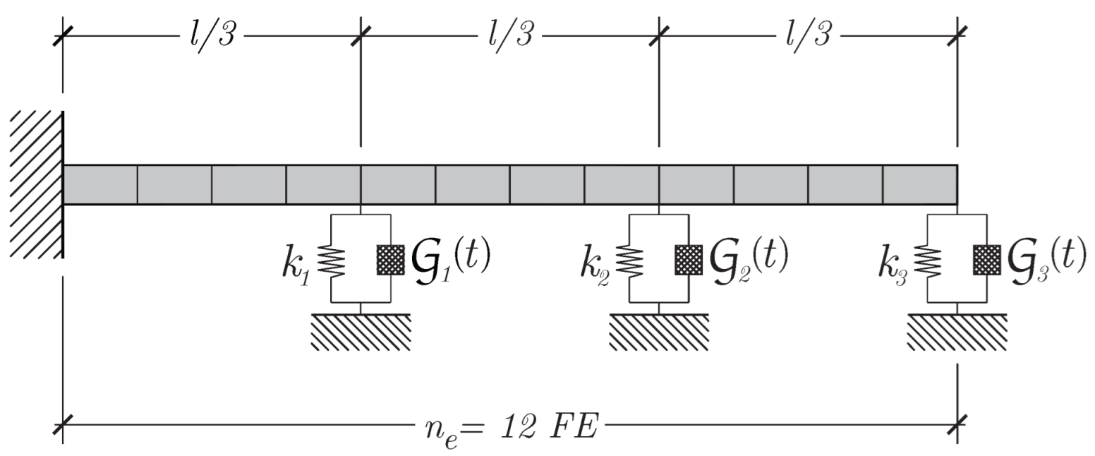
This example is intended to illustrate the application of the method of continuous systems with a higher number of degrees of freedom, in particular, a beam modeled using finite elements. Consider the beam of length $l=5$ m, shown in Figure 6, with simple and clamped supports as boundary conditions, and with three local viscoelastic dampers, placed at sections $l/3,2l/3$, and l, constraining the vertical displacements. A total number of $n_e=12$ two-node Euler–Bernoulli finite elements are used. Each node has three degrees of freedom (two displacements and rotation) resulting in a 36-dof system. The assumed material has a Young modulus $E=210$ GPa and density $\rho =7.85$ t/m${}^3$. The cross section is constant with a flexural stiffness of $EI=224$ kNm${}^2$ and a mass per unit of length of $\rho A=62.8$ kg/m. Each viscoelastic link is formed by a linear spring together with a nonviscous exponential damping function. The stiffness of the springs are $k_1=k_2=3.584$ kN/m and $k_3=7.168$ kN/m. According to the hypothesis assumed in this paper, the three associated exponential kernels ($N=3$) are controlled under three relaxation parameters ${\mu }_k$. Hence, ${\mathcal{G}}_k\left(t\right)={\mu }_k{c}_k{e}^{-{\mu }_{k}t},1\le k\le 3$. The damping model is then a function of three viscous matrices

$$\mathcal{G}\left(t\right)={\mathbf{C}}_1{\mu }_1{e}^{-{\mu }_{1}t}+{\mathbf{C}}_2{\mu }_2{e}^{-{\mu }_{2}t}+{\mathbf{C}}_3{\mu }_3{e}^{-{\mu }_{3}t},$$

(83)

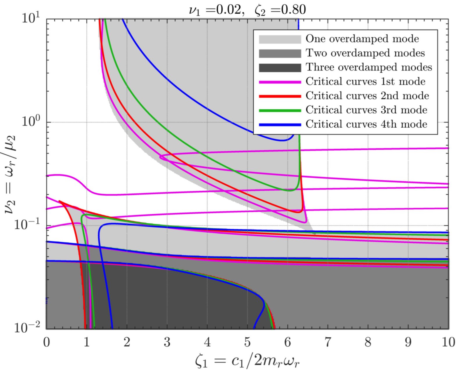
where the matrix ${\mathbf{C}}_k$ has a non-zero element equal to $c_k$ in the entries corresponding to those degrees of freedom that are affected by the kth damper. The parameters will be written, preferably in dimensionless form, as ${\zeta }_k=c_k/2m_r{\omega }_r$ and ${\nu }_k={\omega }_r/{\mu }_k$, where $m_r=314$ kg is the total mass of the beam and ${\omega }_r=\sqrt{EI/m{l}^3}=2.3889$ rad/s is the reference frequency. We propose drawing the critical curves of the parameters $({\zeta }_1,{\nu }_1)$ for the fixed values of the rest of parameters, say $\{{\zeta }_2,{\zeta }_3,{\nu }_2,{\nu }_3\}$. According to the classification given above, this is a type-III curve. Parameters $c_1$ and ${\mu }_1$ are part of the matrix ${\mathbf{C}}_1=c_1{\mathbf{Q}}_1$ and the auxiliary variable ${\mathcal{R}}_{j1}=\alpha /(\alpha -{\omega }_j/{\mu }_1)$, respectively. A derivation of the associated eigenvalue problem is carried out by repeating the process as in the previous example (type-III curves), but considering a greater number of hereditary nuclei. Thus, Equations (52) and (53), after some simplifications, yield:

$${\mathbf{Q}}_1\mathbf{u}=\lambda {\mathcal{B}}_j\mathbf{u},$$

(84)

where:

$${\mathcal{B}}_j={\mathfrak{M}}_j-\sum _{k=2}^N{\mathcal{R}}_{jk}{\mathbf{C}}_k,$$

(85)

and the new parameter $\lambda$ is just a change of the variable of ${\mu }_1$ under the expression:

$$\lambda =-\frac{\left[({\alpha }^2+1){\mathcal{R}}_{j1}-2\right]{\mathbf{\varphi }}_j^T{\mathbf{Q}}_1{\mathbf{\varphi }}_j}{{\sum }_{k=2}^N{\mathcal{R}}_{jk}\left[({\alpha }^2+1){\mathcal{R}}_{jk}-2\right]{\mathbf{\varphi }}_j^T{\mathbf{C}}_k{\mathbf{\varphi }}_j}.$$

(86)

As in previous cases, the curves are obtained by sweeping out the interval $0<\alpha \le 1$ for each mode $1<j<n$. The list of so-determined $\lambda$ values are first transformed into ${\mu }_1$ by Equation (86), and then to $c_1$, knowing that $c_1=1/\left({\mathcal{R}}_{j1}\lambda \right)$. The graphical results are shown in Figure 7, where it can be noticed that taking all modes in structures with a large number of degrees of freedom into consideration is not necessary. Indeed, from a certain mode onwards, the critical curves are covered by the previous modes, so that the pattern of critical regions can be identified by evaluating only a few modes. Thus, in Figure 7, only the first 10 undamped modes have been considered. Among them, the black curves correspond to the fifth and higher modes. This is something that was intuitively manifested in Example 1 and that emerges in the current one as a factor to be taken into account in order to avoid extra computational effort.

As a general trend, the critical regions are identified as the envelope of the curves obtained. After several numerical experiments, the best results are found when overdamped regions occupy a significant part of the domain. When, on the contrary, the regions occupy small, narrow, or isolated areas, the contours generated by our approach may differ from the exact ones. At present, it is not possible to know a priori the general shape of the regions without plotting them, so it is also difficult to diagnose a priori the quality of our approach: both the viscoelasticity and the nonproportionality cannot be evaluated a priori since, for that, we need the value of the damping parameters. Despite these shortcomings, numerical tests show that, in general, the methodology reproduces critical regions quite accurately in a wide range of the parameters, as shown in the exposed numerical examples.

5. Conclusions

In this paper, viscoelastically damped multiple-degrees-of-freedom systems are under consideration. The dissipative model is represented by damping forces with linear dependency of the velocities via hereditary kernel functions. The nature of the response is affected by the parameters of the dissipative model. Some combination of these latter parameters give rise to non-oscillatory modes (overdamped modes). In the damping parametric domain, the thresholds that bound overdamped- and underdamped-induced motion are called critical surfaces (or critical curves when they relate two parameters). New theoretical results have been derived in the form of two theorems. Theorem 1 gives a mathematical characterization of eigensolutions under critical damping, and Theorem 2 relates the location of critical eigenvalues with the nonproportionality of the damping model. In addition, computational tools have been developed, allowing for the discovery of approximations of the critical curves with no restrictions on the number of hereditary kernels for nonproportionally damped systems. The numerical examples show that the quality of the approximation depends on the viscoelasticity of the damping model, defined as a measure of the variation of dissipative functions with frequency. In fact, it has been found that low viscoelasticities lead to a better fit of the boundaries of overdamped regions and the proposed critical curves. The proposal is validated throughout two numerical examples: in the first example, involving a four-dof discrete system, the details to numerically deduce the different types of critical curves are exposed. Overdamped regions are, in general, accurately reproduced, except for cases with notably high viscoelasticity. The second example illustrates the application of our approach to continuous systems, represented by a beam over viscoelastic supports.

References

- Adhikari, S. Dynamics of non-viscously damped linear systems. J. Eng. Mech. 2002, 128, 328–339. [Google Scholar] [CrossRef]
- Adhikari, S.; Woodhouse, J. Identification of Damping: PART 2, Non-Viscous Damping. J. Sound Vib. 2001, 243, 63–88. [Google Scholar] [CrossRef] [Green Version]
- Pritz, T. Analysis of four-parameter fractional derivative model of real solid materials. J. Sound Vib. 1996, 195, 103–115. [Google Scholar] [CrossRef]
- Pritz, T. Five-parameter fractional derivative model for polymeric damping materials. J. Sound Vib. 2003, 265, 935–952. [Google Scholar] [CrossRef]
- Hussein, M.I.; Frazier, M.J. Metadamping: An emergent phenomenon in dissipative metamaterials. J. Sound Vib. 2013, 332, 4767–4774. [Google Scholar] [CrossRef] [Green Version]
- Chen, Y.; Barnhart, M.; Chen, J.; Hu, G.; Sun, C.; Huang, G. Dissipative elastic metamaterials for broadband wave mitigation at subwavelength scale. Compos. Struct. 2016, 136, 358–371. [Google Scholar] [CrossRef]
- Wagner, N.; Adhikari, S. Symmetric state-space method for a class of nonviscously damped systems. AIAA J. 2003, 41, 951–956. [Google Scholar] [CrossRef]
- Lázaro, M. Nonviscous Modes of Nonproportionally Damped Viscoelastic Systems. J. Appl. Mech. 2015, 82, 121011. [Google Scholar] [CrossRef]
- Lázaro, M. Critical damping in non-viscously damped linear systems. Appl. Math. Model. 2019, 65, 661–675. [Google Scholar] [CrossRef] [Green Version]
- Papargyri-Beskou, S.; Beskos, D. On critical viscous damping determination in linear discrete dynamic systems. Acta Mech. 2002, 153, 33–45. [Google Scholar] [CrossRef]
- Bulatovic, R. On the critical damping in multi-degree-of-freedom systems. Mech. Res. Commun. 2002, 29, 315–319. [Google Scholar] [CrossRef]
- Muravyov, A. Forced vibration responses of viscoelastic structure. J. Sound Vib. 1998, 218, 892–907. [Google Scholar] [CrossRef]
- Adhikari, S. Qualitative dynamic characteristics of a non-viscously damped oscillator. Proc. R. Soc. A Math. Phys. Eng. Sci. 2005, 461, 2269–2288. [Google Scholar] [CrossRef]
- Muller, P. Are the eigensolutions of a l-d.o.f. system with viscoelastic damping oscillatory or not? J. Sound Vib. 2005, 285, 501–509. [Google Scholar] [CrossRef]
- Pierro, E. Damping control in viscoelastic beam dynamics. J. Vib. Control. 2020, 26, 1753–1764. [Google Scholar] [CrossRef]
- Wang, P.; Wang, Q.; Xu, X.; Chen, N. Fractional Critical Damping Theory and Its Application in Active Suspension Control. Shock Vib. 2017, 2017, 2738976. [Google Scholar] [CrossRef]
- Lázaro, M. Exact determination of critical damping in multiple-exponential-kernel based viscoelastic single degree-of-freedom systems. Math. Mech. Solids 2019, 24, 3843–3861. [Google Scholar] [CrossRef]
- Lázaro, M. Approximate critical curves in exponentially damped nonviscous systems. Mech. Syst. Signal Process. 2019, 122, 720–736. [Google Scholar] [CrossRef]
- Biot, M. Theory of stress-strain relations in anisotropic viscoelasticity and relaxation phenomena. J. Appl. Phys. 1954, 25, 1385–1391. [Google Scholar] [CrossRef]
- Mohammadi, S.; Voss, H. Variational characterization of real eigenvalues in linear viscoelastic oscillators. Math. Mech. Solids 2018, 23, 1377–1388. [Google Scholar] [CrossRef]
- Mohammadi, S.A.; Voss, H. On the distribution of real eigenvalues in linear viscoelastic oscillators. Numer. Linear Algebra 2019, 26, e2228. [Google Scholar] [CrossRef]
- Lázaro, M.; Pérez-Aparicio, J.L. Characterization of Real Eigenvalues in Linear Viscoelastic Oscillators and the Non-viscous Set. J. Appl. Mech. 2014, 81, 021016. [Google Scholar] [CrossRef]
- Kawano, D.T.; Morzfeld, M.; Ma, F. The decoupling of defective linear dynamical systems in free motion. J. Sound Vib. 2011, 330, 5165–5183. [Google Scholar] [CrossRef] [Green Version]
- Golla, D.; Hughes, P. Dynamics of viscoelastic structures—A time-domain, finite-element formulation. J. Appl. Mech. 1985, 52, 897–906. [Google Scholar] [CrossRef]
- Meirovitch, L. Fundamentals of Vibrations; McGraw Hill: New York, NY, USA, 2001. [Google Scholar]
- Lázaro, M.; García-Raffi, L.M. Critical relationships in nonviscous systems with proportional damping. J. Sound Vib. 2020, 485, 115538. [Google Scholar] [CrossRef]
- Hochstenbach, M.; Kosir, T.; Plestenjak, B. A Jacobi-Davidson type method for the two-parameter eigenvalue problem. SIAM J. Matrix Anal. Appl. 2005, 26, 477–497. [Google Scholar] [CrossRef] [Green Version]
- Muhic, A.; Plestenjak, B. On the singular two-parameter eigenvalue problem. Electron. J. Linear Algebra 2009, 18, 420–437. [Google Scholar] [CrossRef] [Green Version]
Figure 1.
The four-degrees-of-freedom discrete system of Example 1, with nonproportional damping. and represent the hereditary function of nonviscous dampers. Masses kg; rigidities N/m.
Figure 2.
Proposed critical curves of Example 1, for four different cases of nonviscous parameters . Gray-shaded areas represent exact overdamped regions: the darker the gray color the greater the number of overdamped modes.
Figure 3.
Critical curves of the four-degrees-of-freedom discrete system of Example 1 with , . Shaded regions represent the exact critical regions. The different levels of gray color stands for the number of overdamped modes.
Figure 4.
Critical curves of the discrete four-dof model of Example 1, in the domain of the two parameters (viscous and nonviscous parameters of the second kernel). The rest of the parameters are and . Grayscales show regions with one and two overdaped modes.
Figure 5.
Critical curves of the four-dof discrete system of Example 1 in the domain of parameters (viscous ratio of the first kernel and nonviscous parameters of the second kernel). Other parameters: and .
Figure 6.
Continuous beam of Example 2, with 12 Euler–Bernouilli-like finite elements and three different viscoelastic supports with hereditary functions .
Figure 7.
(Example 2) Critical curves of parameters for two different combinations of the rest of the parameters (shown on the top of each plot).