Improving the Performance of Convolutional GAN Using History-State Ensemble for Unsupervised Early Fault Detection with Acoustic Emission Signals

Abstract

Early fault detection (EFD) in run-to-failure processes plays a crucial role in the condition monitoring of modern industrial rotating facilities, which entail increasing demands for safety, energy and ecological savings and efficiency. To enable effective protection measures, the evolving faults have to be recognized and identified as early as possible. The major challenge is to distil discriminative features on the basis of only the ‘health’ signal, which is uniquely available from various possible sensors before damage sets in and before the signatures of incipient damage become obvious and well-understood in the signal. Acoustic emission (AE) signals have been frequently reported to be able to deliver early diagnostic information due to their inherently high sensitivity to the incipient fault activities, highlighting the great potential of the AE technique for EFD, which may outperform the traditional vibration-based analysis in many situations. To date, the ‘feature-based’ multivariate analysis dominates the interpretation of AE waveforms. In this way, the decision-making relies heavily on experts’ knowledge and experience, which is often a weak link in the entire EFD chain. With the advent of artificial intelligence, practitioners seek an intelligent method capable of tackling this challenge. In the present paper, we introduce a versatile approach towards intelligent data analysis adapted to AE signals streaming from the sensors used for the continuous monitoring of rotating machinery. A new architecture with a convolutional generative adversarial network (GAN) is designed to extract the deep information embedded in the AE waveforms. In order to improve the robustness of the proposed EFD framework, a novel ensemble technique referred to as ‘history-state ensemble’ (HSE) is introduced and paired with GAN. The primary merits of HSE are twofold: (1) it does not require extra computing time to obtain the base models, and (2) it does not require a special design of the network architecture and can be applied to different networks. To evaluate the proposed method, a durability rolling contact fatigue test was performed with the use of AE monitoring. The experimental results have demonstrated that the proposed ensemble method largely improves the robustness of GAN.

1. Introduction

A rolling bearing is the core component in many rotating machines. Any failure in rolling bearings can lead to a chain reaction of faults in the whole mechanical system, causing the rapid and unexpected breakdown of the machine. Being an essential part of condition monitoring, the early and accurate identification of an imminent failure is deemed effective in reducing property loss and even possible casualties caused by catastrophic industrial breakdowns. Recent years have seen the rapid development of innovative artificial intelligence (AI) algorithms, including two major groups: machine learning (ML) and deep learning (DL). Inspired by the progress in this field on the one hand, and informed by the long-standing unaddressed challenges faced by traditional ‘feature-based’ approaches, practitioners strive to find new solvers—intelligent methods capable of detecting the emerging faults early, reliably and seamlessly, without heavy reliance on human labor and expert experience [1,2]. To date, numerous intelligent fault diagnosis schemes have been proposed. Lei et al. have analyzed the relevant bibliometric data in this field [2]. The application of DL started to thrive after 2015 and it gradually surpassed traditional ML models. At present, the DL-based machine fault diagnosis framework has become the mainstream of intelligent fault diagnostics. Compared with traditional ML models, the procedures of feature extraction and fault recognition are integrated within the DL approach. The DL approach is unique in that it is capable of extracting features automatically from the input data through multiple layers comprising processing units called hidden neurons. This makes DL suitable to process the raw signal straightforwardly, without any signal pre-processing. Classical DL architectures include the Back Propagation Neuron Network (BPNN) [3], Convolutional Neuron Network (CNN) [4,5], Deep Boltzmann Machine (DBM), Deep Brief Network (DBN), Autoencoder (AEN) [6,7], Long Short-Term Memory (LSTM) network [8,9] and their variants.

The emerging damage in the machine can be communicated through different signal sources. Among them, the vibration-based technique is the most widely used one owing to its simplicity, the transparency of the analysis based on spectral features and cost advantages. However, there are shortcomings of vibration signals, which are to be mentioned. Firstly, the vibration acceleration signals can hardly be detectable until the damage develops significantly to a mature stage, corresponding to large-scale faults causing vibrations in heavy or slowly rotating structures. It is often too late to use this information for preventive maintenance [10]. Secondly, the vibration signals induced by early defects are easily masked by the routine background mechanical vibration of the rotating machine. It has been frequently reported that acoustic emission (AE) signals can detect the incipient crack earlier than traditional vibration signals [11,12,13,14]. Even if this claim is not always justified, the modern AE technique provides a promising means for EFD in roller bearings. The AE is referred to as a phenomenon of transient elastic wave generation by a sudden local drop in internal stress within the material. Compared to the vibration signal, AE has a much wider frequency range (20 kHz to 10 MHz), and, thus, it does not overlap or interfere with low-frequency mechanical vibration signals. To date, the ‘feature-based’ parametric analysis prevails in interpreting information derived from AE waveforms [15,16,17]. However, these hand-designed features are inherently linked through AE to the specific signal processing techniques in the time, frequency or time–frequency domains [15,18,19]. These features need to be carefully extracted and analyzed by experts, and there is no guarantee that the features tailored to a specific fault diagnosis condition are applicable for other tasks.

To reduce the risk of biased opinions, we leverage the DL technique to explore the implicit fault information embedded in AE signals. Among all types of DL models, the generative adversarial network (GAN) has shown a remarkable capacity to perform distribution fitting. GAN is a powerful generative model that was first proposed by Goodfellow et al. in 2014 [20]. Unlike conventional neural networks, GAN implements generative modeling as a game between two separated networks: a Generator is trained to produce synthetic data that are close to the real data, while a Discriminator is trained to discriminate between the synthetic and real data. During this training process, the probability distribution of the real data can be learned by the Generator. There are many successful applications of GAN in the fault diagnosis field. Existing research mainly focuses on the problem of ‘unbalanced data’, i.e., the sample size of anomal data is much smaller than that of regular data [21,22,23,24,25,26]. GAN is utilized to generate synthetic abnormal data to assist model training. These studies have demonstrated that GAN has an excellent ability to learn representative features from mechanical signals. Xia et al. summarized the applications of GAN to anomaly detection in a number of fields [27]. It can be concluded that GAN is suitable for early fault detection (EFD) problems in two ways [28]: (1) it shows superiority in fitting the distribution of health signals; the Generator can be trained to learn rich and hierarchical information from the data characteristic of the normal operating state of the machine; thus, these abnormal data should be poorly reconstructed; (2) the Discriminator forms a health indicator (HI) to indicate the abnormal signals.

Although GAN is a promising approach for EFD, it faces a well-known issue of unstable training. In contrast to traditional supervised networks, whose performance can be well reflected by the loss value, GAN consists of two networks’ fighting’ with each other, so the loss values of the two networks show a relationship of ‘as one falls, the other rises’. The balance between the Generator and Discriminator is subtle. Therefore, it is difficult to determine when the Discriminator is well-trained, leading to the problem of instability. In order to improve the robustness of GAN in the EFD problem, we introduced a new ensemble technique referred to as the ‘history-state ensemble’ (HSE) [29] method. HSE assumes that neural networks can generate multiple local optima during the training history. Our previous experimental results [29] have demonstrated that these local optima are diverse, and their combination improves the accuracy and stability of the single network. The ensemble method is generally perceived to be time-consuming. However, the benefit of the HSE is that it does not require extra training costs to obtain multiple base models. We only need to record the historical training model weights that should be discarded after each model update when using the backpropagation algorithm to adjust the model. Therefore, it does not require a specially designed network architecture. These historical training model weights are denoted as ‘history states’ or base models.

In a brief summary, the main contributions of this paper are as follows.

(1)

We proposed a novel architecture of GAN consisting of convolutional blocks and LSTM for EFD in the run-to-failure process.

(2)

A new ensembled health indicator (EHI) is constructed by integrating GAN and a novel ensemble technique called the HSE method.

(3)

A laboratory durability test of a roller bearing element monitored by the acoustic emission technique was carried out to evaluate the effectiveness of the proposed method.

2. The Proposed Architecture of Convolutional GAN

We first introduce the basic theory of traditional GAN, and the architecture of the proposed convolutional GAN is elaborated.

2.1. Basic Theory of GAN

The basic structure of GAN consists of two networks, as illustrated in Figure 1. The main idea is to construct a neural network model, known as the ‘Generator’, in order to map the random noises $\mathit{z}$ into a new data space $G\left(\mathit{z}\right)$. The goal is to minimize the discrepancy between the ‘fake data’ from the mapped space $G\left(\mathit{z}\right)$ and the ‘real data’ from the target space $p_r\left(\mathit{x}\right)$. In contrast to traditional neural networks such as the Autoencoder, which directly minimizes the distance through the mean square error (MSE), one more neural network is introduced in GAN, referred to as the ‘Discriminator’, which is aimed to distinguish $G\left(\mathit{z}\right)$ from $p_r\left(\mathit{x}\right)$.

The above stated goal can be achieved through the joint training of the two networks, and the original loss functions for the Generator and Discriminator are express as follows:

$$\underset{D}{\max }L\left(D\right)=E_{\mathit{x}\sim p_r\left(\mathit{x}\right)}\left[logD\left(\mathit{x}\right)\right]+E_{\mathit{z}\sim p_z\left(\mathit{z}\right)}\left[log\left(1-D\left(G\left(\mathit{z}\right)\right)\right)\right]$$

(1)

$$\underset{G}{\min }L\left(G\right)=E_{\mathit{z}\sim p_z\left(\mathit{z}\right)}\left[log\left(1-D\left(G\left(\mathit{z}\right)\right)\right)\right]$$

(2)

where $G$ and $D$ represent the Generator and Discriminator, respectively. The $D$ outputs a score ranging from 0 to 1 for each sample. In order to distinguish between the ‘fake data’ and ‘real data’, $D$ tries to assign a value close to 1 for the sample $\mathit{x}$ from ‘real data’, and a value close to 0 for the sample $G\left(\mathit{z}\right)$ from ‘fake data’. Then, the loss function for $D$ is maximized. On the other hand, $G$ attempts to produce ‘fake data’ to fool $D$; thus, it will be adjusted to produce ‘fake data’ that are close to ‘real data’, allowing $D\left(G\left(\mathit{z}\right)\right)$ to be close to 1; therefore, the loss function of $G$ is minimized. If both networks have sufficient capacity, they will reach a point at which both models cannot be improved anymore because the generated distribution approximates the real distribution well enough.

The original loss function of GAN has been reported with challenges, such as unstable training and the poor quality of generated data. The key problem stems from the embedded Jensen–Shannon divergence (JSD) as a measure of the distance between real and generated distribution; the details can be found in [30]. To overcome the training challenges, Arjovsky et al., proposed to replace JSD with the Wasserstein distance (WD) defined as

$$W\left(p_r,p_{\theta }\right)=\frac{1}{K}su{p}_{{\Vert f\Vert }_L\le 1} E_{\mathit{x}\sim p_r}\left[f\left(\mathit{x}\right)\right]-E_{\tilde{\mathit{x}}\sim p_g}\left[f\left(\tilde{\mathit{x}}\right)\right]$$

(3)

where $f:\mathit{x}\to R$ is a set of Lipschitz functions satisfying the condition $\frac{\left|f\left(x_1\right)-f\left(x_2\right)\right|}{\left|x_1-x_2\right|}\le K$, and $K$ is the Lipschitz constant. It can be observed that the absolute value of the derivative of $f$ does not exceed $K$. By applying this distance metric in GAN, the function $f$ is referred to as a ‘critic’ in the original paper, which can be approximated by $D$, and $p_g$ is the model distribution implicitly defined by $\tilde{\mathit{x}}=G\left(\mathit{z}\right)$, $\mathit{z}\sim p_z\left(\mathit{z}\right)$. The variant of GAN with WD is known as Wasserstein GAN (WGAN). Compared with JSD, WD has a smoother change rate when measuring the distance between two distributions; thus, it can provide meaningful gradient information to $G$.

The original WGAN applies a ‘weight clipping’ method to enforce a Lipschitz constraint by clamping the network weights to a fixed range $\left[-c,c\right]$ after each gradient update. This method still leads to optimization difficulties such as gradient vanishing [23,31]. Therefore, Gulrajani et al. proposed an alternative solution by enforcing a soft version of the Lipschitz constraint with a penalty on the gradient norm of random samples $\check{\mathit{x}}\sim p_{\check{\mathit{x}}}$, which is expressed as

$$\delta =E_{\tilde{\mathit{x}}\sim p_{\tilde{\mathit{x}}}}\left[{\left(\Vert {\nabla }_{\tilde{\mathit{x}}}D{\left(\tilde{\mathit{x}}\right)\Vert }_2-K\right)}^2\right]$$

(4)

where $\check{\mathit{x}}=\epsilon \mathit{x}+\left(1-\epsilon \tilde{\mathit{x}}\right)$, with $\mathit{x}\sim p_r$, $\tilde{\mathit{x}}\sim p_g$, and $\epsilon \sim N\left[0,1\right]$. The $K$ is generally set as 1.

With the gradient penalty, a new objective is proposed as

$$\underset{D}{\max }L\left(D\right)=E_{\tilde{\mathit{x}}\sim p_{\theta }}\left[D\left(\tilde{\mathit{x}}\right)\right]-E_{\mathit{x}\sim p_r}\left[D\left(\mathit{x}\right)\right]+\beta E_{\tilde{\mathit{x}}\sim p_{\tilde{\mathit{x}}}}\left[{\left(\Vert {\mathit{\nabla }}_{\tilde{\mathit{x}}}D{\left(\tilde{\mathit{x}}\right)\Vert }_2-1\right)}^2\right]$$

(5)

$$\underset{G}{\min }L\left(G\right)=-E_{\tilde{\mathit{x}}\sim p_{\tilde{\mathit{x}}}}\left[D\left(\tilde{\mathit{x}}\right)\right]$$

(6)

where $\beta$ is the penalty coefficient, and the WGAN with a gradient penalty is referred to as gp-WGAN.

2.2. Design of Generator and Discriminator

It is well-known that GAN is difficult to train, even with the use of WD and gradient penalty methods. One of the prime challenges is the diversity of the generated data, which is needed to cover the data distribution sufficiently. Otherwise, the Generator may become ‘lazy’, therefore producing the homogeneous data fooling the Discriminator. However, a good point in early fault detection, i.e., in early anomaly detection in the streaming of diagnostic data, is that the primary focus should be the performance of the Discriminator. This is the difference between our task and many other tasks, such as image generation or imbalanced data problems in fault diagnostics. In our work, it is not necessary that the Generator’s input is a random signal. Hence, the Autoencoder-based Generator architecture is adopted in this work, i.e., both the input and output of the Generator are real data. The Autoencoder is known as a powerful and versatile non-linear dimensionality reduction technique employing neural networks for which the target output is the same as the input.

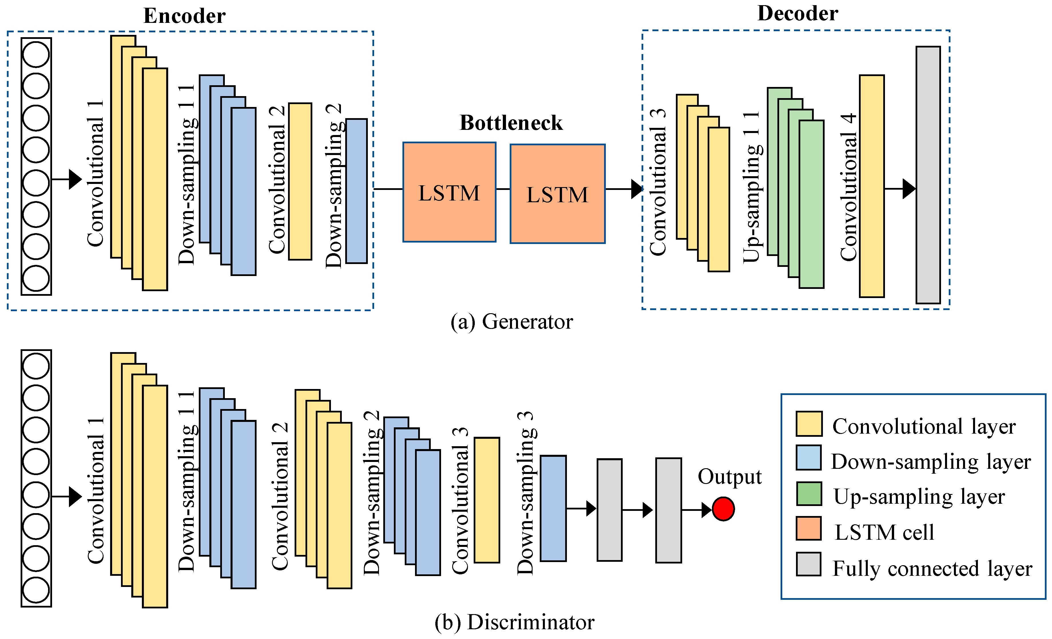
The proposed architectures of the Generator and Discriminator are shown in Figure 2. The Generator comprises an encoder block and a decoder block with a bottleneck block between them. The encoder is built of two convolutional layers to learn hierarchical representations of the real input, and each convolutional layer is followed by a down-sampling layer to reduce the feature size. Moreover, the down-sampling layer helps to boost the model’s robustness to noise and variations in input data. Then, the real input is compressed into a compact representation called the bottleneck. In this paper, the LSTM cell is used in the bottleneck layer to capture the time-series correlation in data. By stacking two layers of LSTM cells, the network can learn more complex patterns in the input data and have better long-term memory retention. Next, the compressed representation is fed into the decoder, which consists of two convolutional layers, one up-sampling layer and one fully connected layer that finally reconstructs the input. In the competition between the Generator and the Discriminator, if the Discriminator is too powerful, it will quickly converge before the Generator can learn useful information from the input. Therefore, a more concise structure is used in the Discriminator, which is composed of three convolutional layers, three down-sampling layers, two fully connected layers and a one-dimensional output layer.

The most important mathematical details related to the above structure are presented below.

(1)

Convolutional layer. The convolution process refers to a specialized linear operation where a small window called a kernel or filter overlays and slides through the entire input with a preset stride, which is mathematically expressed as

$${\mathit{H}}_k=Activ\left({\displaystyle \sum }_{i=1}^{inMap}Conv\left({\mathit{W}}_k, {\mathit{X}}_i\right)+b_k\right)$$

(7)

where $Conv\left(\cdot \right)$ denotes the convolution window, ${\mathit{W}}_k$ is the kernel that slides through the data $\mathit{X}$ and $b_k$ is the corresponding bias. $Activ\left(\cdot \right)$ represents the activation function, ${\mathit{H}}_k$ stands for the feature vector extracted by the k-th kernel and the subscript k defines the number of kernels.

(2)

Average down-sampling layer. The down-sampling layer is also referred to as the pooling layer, which is commonly applied after a convolution layer to reduce the dimension of the feature maps. It refers to a special type of convolution whereby the kernel slides through the entire input map, and, generally, instead of creating the element-wise product, the average value of the overlaid input region is extracted; this quantity is the so-called ‘average pooling’.

(3)

Up-sampling layer. In contrast to down-sampling, up-sampling is generally used after the encoder to restore the resolution of the original data. The most common up-sampling techniques include Nearest Neighbor, Bilinear and Bicubic [32]. The Bilinear method is adopted in the present work.

(4)

Fully connected layer. The fully connected layer refers to the type of neural network where all the input from the previous layer is connected to every neural node of the next layer:

$$\widehat{\mathit{H}}=\mathrm{Activ}\left(\mathit{W}\ast \mathit{H}+b\right)$$

(8)

where $\mathit{H}$ stands for the neural nodes of the previous layer; $\mathit{W}$ and $b$ represent the weights and bias.

(5)

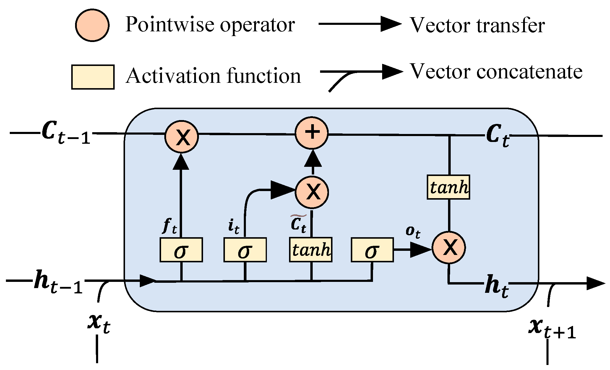
LSTM cell. LSTM is a variant of Recurrent Neural Network (RNN), which has the advantage of exploiting the information of time-series signals. LSTM alleviates the vanishing gradient problem in the original RNN by introducing a memory cell, as described in Figure 3. The memory cell consists of a forget gate, input gate, output gate and state gate, which are mathematically described as follows:

$${\mathit{f}}_t=\sigma \left({\mathit{W}}_f·\left[{\mathit{x}}_t, {\mathit{h}}_{t-1}\right]+b_f\right)$$

(9)

$${\mathit{i}}_t=\sigma \left({\mathit{W}}_i·\left[{\mathit{x}}_t, {\mathit{h}}_{t-1}\right]+b_i\right)$$

(10)

$${\mathit{o}}_t=\sigma \left({\mathit{W}}_o·\left[{\mathit{x}}_t, {\mathit{h}}_{t-1}\right]+b_o\right)$$

(11)

$$\widetilde{{\mathit{C}}_t}=tanh\left({\mathit{W}}_c·\left[{\mathit{x}}_t, {\mathit{h}}_{t-1}\right]+b_c\right)$$

(12)

$${\mathit{C}}_t={\mathit{f}}_t·{\mathit{C}}_{t-1}+{\mathit{i}}_t·\widetilde{{\mathit{C}}_t}$$

(13)

$${\mathit{h}}_t={\mathit{o}}_t·tanh\left({\mathit{C}}_{t-1}\right)$$

(14)

where the ${\mathit{f}}_t$, ${\mathit{i}}_t$, ${\mathit{o}}_t$ and ${\mathit{C}}_t$ represent the forget gate, input gate, output gate and state gate, respectively. ${\mathit{x}}_t$ is the input vector of the LSTM unit at the current time $t$, and ${\mathit{h}}_{t-1}$ is the hidden vector of the previous time $t-1$. Therefore, LSTM considers the information at the current time and the previous time. $\sigma$ and $tanh$ represent the ‘sigmoid’ and ‘tanh’ activation functions, respectively.

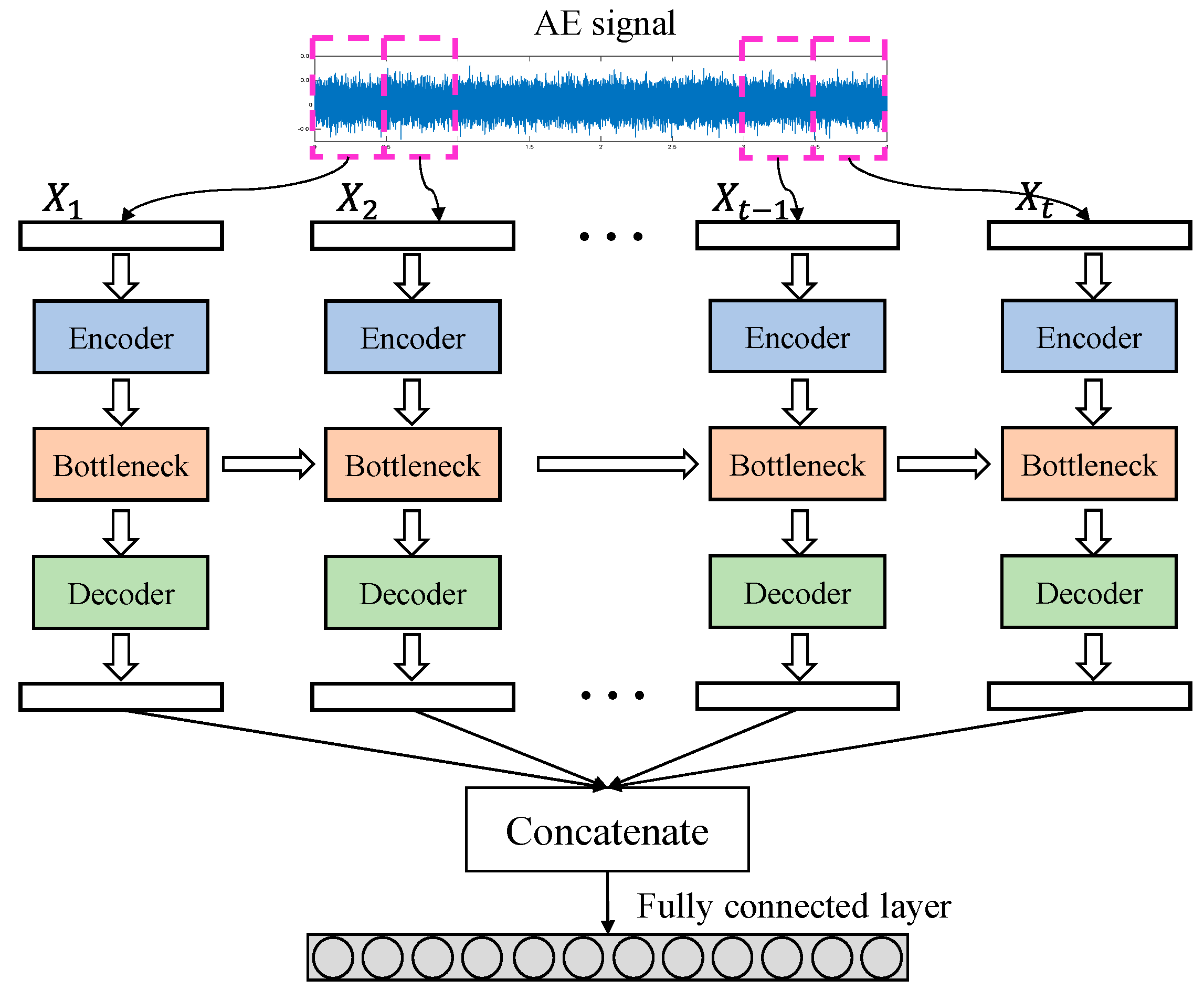
It is worth noting that the input of LSTM should be a matrix, but the AE signal is a vector. Thus, the original 1D data should be converted to two-dimensional space. To this end, we simply divide the signal into multiple segments along the time axis. Thus, the input is reshaped into a $N\times M$ matrix, where $N$ denotes the number of segments, and $M$ stands for the length of each segment. The matrix is firstly processed by the encoder as $M$ separated samples to capture detailed information about each segment, and the extracted features are stacked as a matrix and fed into the bottleneck layer. The output of the bottleneck layer is again processed by the decoder as a separate dataset. The reconstructed data are concatenated by the last fully connected layer. The data flow in the Generator is illustrated in Figure 4.

3. The Proposed EFD Framework Based on Convolutional GAN and History-State Ensemble

3.1. Definition of a Health Indicator (HI) Based on GAN

The output of the Discriminator is a single value that distinguishes the fake data from real data. If the input is identified as real, the Discriminator will ascribe a high value to it, whereas a low value will be set otherwise. If we apply this to the early fault detection problem with the training data from only the normal operating state, the Discriminator will ascribe the faulty data to the low value based on the assumption that the defect has distorted the normal AE waveform, which is successfully captured by the sensors. Therefore, the Discriminator naturally determines the health indicator HI, as presented below:

$$HI=D\left(\mathit{X}\right)$$

(15)

where $\mathit{X}$ denotes the evaluated data.

3.2. Ensembled Health Indicator

3.2.1. Motivation

The remaining question is how to determine whether the Discriminator has been well-trained or not. Differing from traditional supervised networks, whose performance can be assessed by the loss value, GAN benefits from the competition between the Generator and Discriminator. Therefore, the loss values of the two networks exhibit a relation of ‘as one falls, the other rises’. To overcome this problem, we introduce a simple yet effective ensemble technique referred to as the history-state ensemble (HSE) method, as described in our dedicated study [29]. The advantages of the HSE method are twofold: (1) it does not require extra computing time to obtain the base models, and (2) it is versatile enough to be seamlessly applied to plain neural networks without readjusting the network architecture. Similarly to traditional ensemble techniques, the implementation of HSE methods assumes (i) encouraging the model to generate accurate base models with high diversity, and (ii) assembling these models to create a more robust classifier.

3.2.2. Base Model Generation

To obtain the base models, HSE is based on the assumption that the neural networks can generate multiple local optima, also referred to as ‘history states’, during the training process, and these local optima can be taken as base models for ensemble learning. Therefore, to generate multiple base models, one only needs to preserve the historical weights of the network, as illustrated in Figure 5. Hence, the time cost of this procedure is negligible.

The obtained base models have a direct impact on the model performance, which is affected chiefly by three factors: (1) the number of base models, (2) the accuracy of each base model and (3) the diversity within all base models. In order to encourage the diversity of base models, the Mini-Batch Gradient Descent (MBGD) is recommended in the training process. MBGD is a variant of the gradient descent algorithm whereby the whole training dataset is divided into multiple small batches, and only one batch is used to calculate the gradient at each iteration. The application of MBGD increases the model update frequency, which helps to generate more models and encourages their diversity. Moreover, two extra parameters need to be defined, as illustrated in Figure 5. Here, ${\theta }_1$ denotes the number of training epochs at which the first base model is acquired, and ${\theta }_2$ indicates the model update frequency. The total number of acquired base models is calculated as

$$N=int\left(\frac{S-{\theta }_1}{{\theta }_2}\right)$$

(16)

where S is the total number of training epochs.

3.2.3. Ensemble Results

Average voting (AV) is used to integrate the results of all base models, and, for the case of this paper, a new ensembled HI (EHI) can be constructed:

$$EHI={\displaystyle \sum }_{i=1}^N{D}_i\left(\widehat{\mathit{X}}\right)/N$$

(17)

where $D_i\left(\widehat{\mathit{X}}\right)$ represents the score given by the i-th base model, and $N$ is the total number of the base models.

To define the fault alarm, a threshold $th$ is set as

$$th=min\left(EH{I}_{train}\right)-C\ast std\left(EH{I}_{train}\right)$$

(18)

where $H{I}_{train}$ represents the HI values obtained by training signals. $min\left(·\right)$ selects the minimum value of all the $H{I}_{train}$ values, and $std$ represents the standard deviation. $C$ is the constant that reflects the confidence of the result. In this paper, the $C$ is set as 3.

3.3. Dimension Reduction of the Raw AE signals

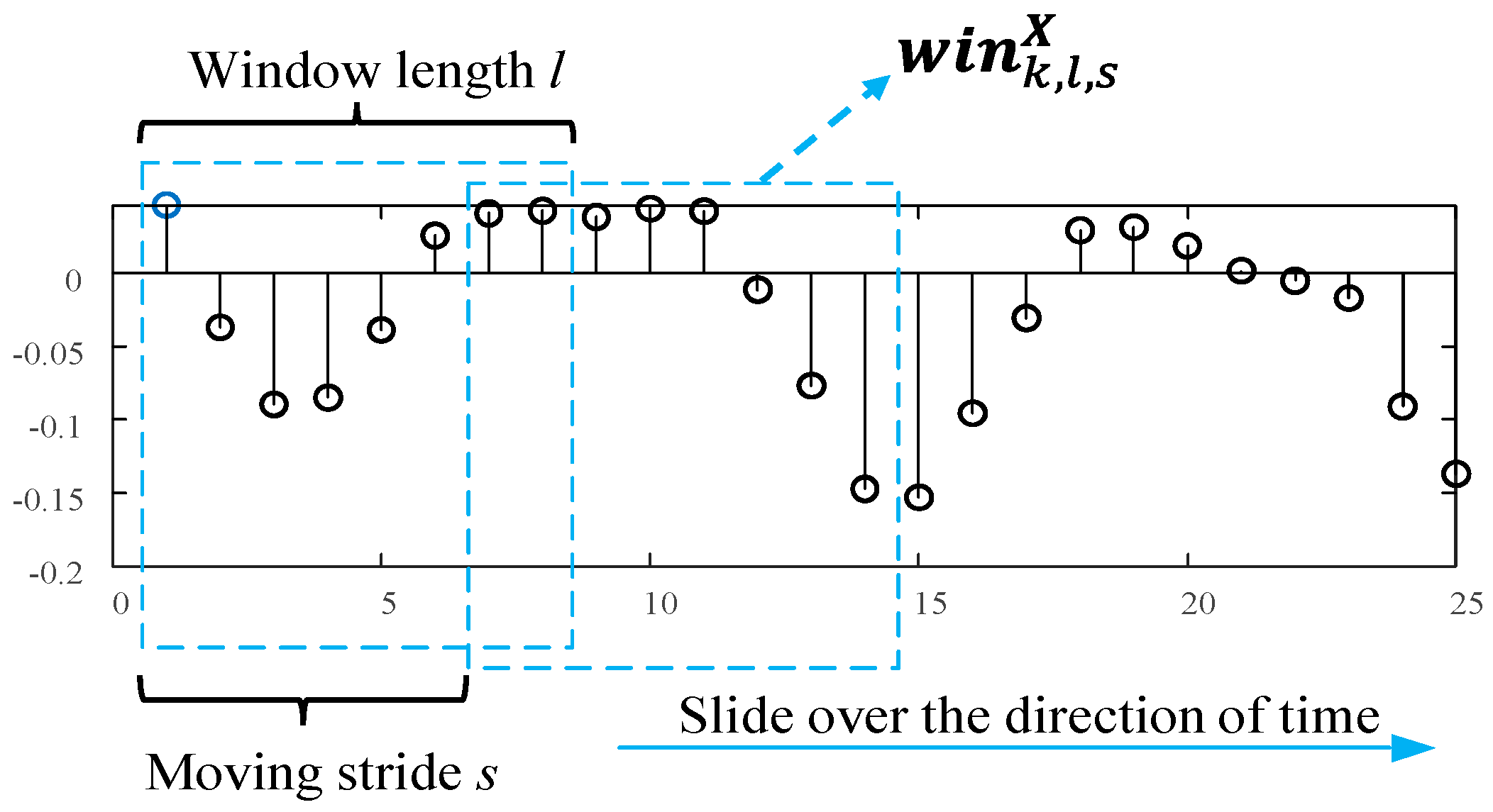
The high sampling frequency of AE signals results in a large amount of acquired data, which increases the computational burden of the model. Therefore, a Moving Variance Window (MVW) is applied to the raw AE signals for dimension reduction, as illustrated in Figure 6. With the step-wise shifting of the window, the variance of the covered signal is calculated, i.e., each windowed data segment is transformed into a single value of the variance. The output is a dimensionless number, which measures the dispersion of the data; thereby, the sub-signal is de-dimensionalized. The function of MVW is to capture the transient events and highlight some essential detailed features of the data. Moreover, since the signal dimension is vastly reduced, processing by the neural network is faster and easier. The MVW is mathematically described as follows:

$$\widehat{\mathit{X}}=\frac{1}{l}{\displaystyle \sum }_{\mathit{x}\in \mathit{w}\mathit{i}{\mathit{n}}_{k,l,s}^{\mathit{X}}}{\left|\mathit{x}-\mu \right|}^2$$

(19)

$$\mathit{w}\mathit{i}{\mathit{n}}_{k,l,s}^{\mathit{X}}=\mathit{X}\left[x_{start}^{k,s}:x_{start}^{k,s}+l-1\right]$$

(20)

$$x_{start}^{k,s}=\left(k-1\right)\times s+1, k=1,2,\dots n_k$$

(21)

where $\mathit{X}$ denotes the raw AE signal, $\mathit{w}\mathit{i}{\mathit{n}}_{k,l,s}^{\mathit{X}}$ represents the area of signal $\mathit{X}$ covered by the moving window, and $k$, $l$ and $s$ are integers specifying the moving step, window length and moving stride, as illustrated in Figure 6. $x_{start}^{k,s}$ is the start point of the window on signal $\mathit{X}$. The total number of moving steps is computed as $n_k=\left[\left(N-l\right)/s\right]+1$, where $N$ is the length of the recorded AE signal; $\mu$ in definition (19) denotes the mean of $\mathit{w}\mathit{i}{\mathit{n}}_{k,l,s}^{\mathit{X}}$. The MVW applies a moving window slide over the original AE signal to extract the variance; thus, the signal dimension can be largely reduced, which makes it easier to be processed by the neural network. Additionally, the MVW helps to capture the transient events and highlight some important detailed information in the data.

3.4. Overall Framework

With the pre-processing of dimensional reduction, the original high-dimensional AE signals can be processed by the proposed ensembled convolutional GAN. The general procedures of the proposed EFD framework are summarized as follows.

Step 1: Data acquisition. AE signals are acquired at fixed time intervals from sensors mounted on the test machine. The signals received at the initial health stage of the experiment are treated as the training set, and the remaining serve as the test set.

Step 2: Dimension reduction The MVW is first applied to the raw signals to reduce the dimension.

Step 3: Model set-up.

(1)

Offline training stage: the pre-processed training data are fed into the convolutional GAN. During the training phase, the history states are recorded at fixed training epochs. Thus, N base models are obtained.

(2)

Setup threshold: the training set is fed into the Discriminator only, and N scores are generated by the base models for each sample. The EHI and the threshold are calculated by Equations (17) and (18).

Step 4: Online test stage. The samples in the test set are sequentially fed into the Discriminator to calculate the $EHI$. The $EHI$ values exceeding the threshold are considered a fault alarm.

4. Experimental Validation

4.1. Test Rig and AE Data Acquisition

One can find more details of the experimental setup and durability test in [17]. To evaluate the performance of the proposed method, a rolling contact fatigue test was carried out in this section. The test rig, designed at SINTEF Industry (Trondheim, Norway), consists of four roller bearings, as illustrated in Figure 7a. The test specimen is in the central position, supported by another three rollers. Each roller is supported by two needle bearings (type SKF NA 6914-zw). To monitor damage associated with the rolling contact fatigue, the broadband WD (MISTRAS, Princeton, NJ, USA) sensors were mounted on the housing of the needle bearing supporting the test roller. A close-up view of the sensors and their location on the rig is presented in Figure 7b. The streaming AE signals were recorded periodically at fixed time intervals, and each data file contains 2 s of streaming AE waveforms sampled at 2 MHz using the Kongsberg HSIO-100-A (Kongsberg Maritime, Trondheim, Norway) high-speed acquisition module. At the beginning of the test, the recording time interval was set at 60 min. When the first damage was confirmed by periodic ultrasonic inspections of the test roller, the recording time interval was reduced to 20 min to obtain more AE realizations containing information about the faults. At the end of the experiment, 2471 AE records were qualified for the analysis. Figure 8 displays the amplitude of the raw AE signal against contact fatigue cycles. An appreciable change in the AE amplitude is observed for the first time after 4.6 × 10⁷ fatigue cycles.

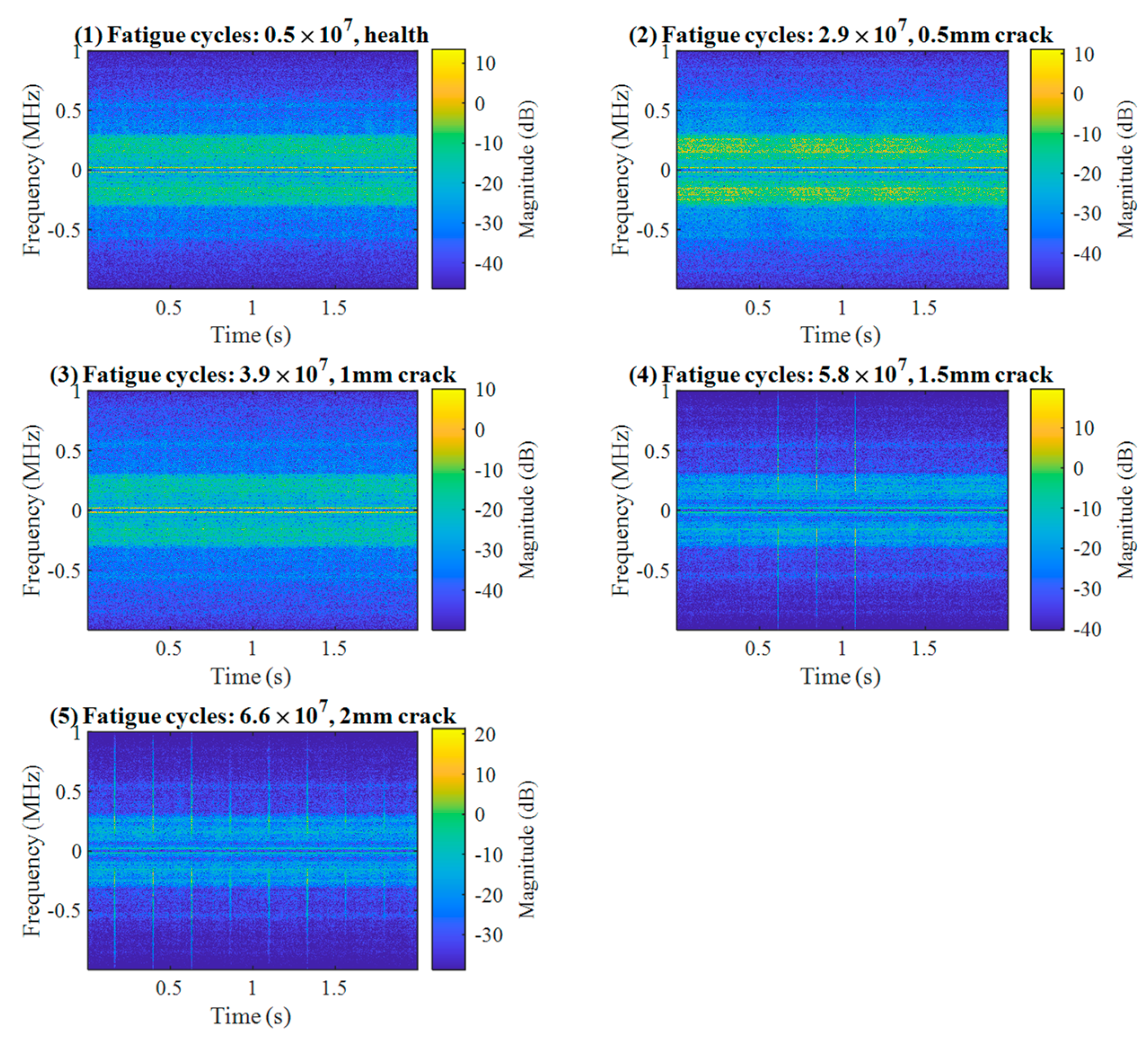
To monitor and visualize the development of incipient damage, ultrasonic inspections were performed periodically during the test using the Olympus OMNISCAN SX (Olympus, Tokyo, Japan) phase array ultrasonic tester (PAUT). According to the PAUT inspection results, the health condition of the test specimen was divided into five stages, as indicated by different colors in Figure 8. The number of records for each state is presented in

Table 1. The number of AE records for different stages of damage propagation.

Health Condition	Number of Records	Number of Fatigue Cycles
No damage	542	2.8 × 107
0.5 mm crack	377	3.6 × 107
1 mm crack	809	4.8 × 107
1.5 mm crack	718	6.5 × 107
2 mm crack	25	6.6 × 107

. The short-time Fourier spectrograms of several randomly chosen AE signals, which are typically observed during the five stages of the damage propagation, are presented in Figure 9. It can be seen that the fault signatures at the early stage of the damage (corresponding to 0.5 mm and 1 mm length of the internal crack) are still invisible to the naked eye. As the faults grow up to 1.5 mm, some high-frequency components induced by AE bursts emerge gradually, and the number of AE bursts increases with the damage development.

4.2. Results and Discussion

4.2.1. Data Preprocessing

Original high-dimensional AE signals are firstly processed by MVW with the moving step $k$ of 8192. The window length $l$ and moving stride $s$ are set as 464. Therefore, each AE file is downsized to a shorter vector with a length of 8192. Let us recall the structure of the Generator, where two LSTM cells are utilized to capture the time-series correlations in the data. To fit the Generator, each input datum is divided into $N$ segments with length $M$, as described in Figure 4. We recommend that each segment should contain information about at least one entire axel revolution. In this way, LSTMs can capture the correlation of AE signals generated in continuous axel revolutions. For instance, the lowest axel rotation frequency in the present work is 254 rpm, i.e., for a 2-s recording, 8 complete rotations are captured. Therefore, the segment parameters $N$ and $M$ are defined as 8 and 1024, respectively.

4.2.2. Network Training

The proposed method was implemented with the open-source PyTorch machine learning framework. The detailed architectures of the proposed Generator and Discriminator are described in

Table 2. The detailed parameters of the proposed Generator and Discriminator.

Generator		Discriminator
Layers	Output size	Layers	Output size
$Input$	$1024@1$	$Input$	$8192@1$
$\left[C:25,S:1,P:12\right]$	$1024@16$	$\left[C:125,S:1,P:63\right]$	$8192@8$
$\left[\begin{array}{c}A:2,S:2,P:0\\ Batchnorm\end{array}\right]$	$512@16$	$\left[A:2,S:2,P:0\right]$	$4096@8$
$\left[C:5,S:1,P:2\right]$	$512@1$	$\left[C:25,S:1,P:12\right]$	$4096@16$
$\left[\begin{array}{c}A:2,S:2,P:0\\ Batchnorm\end{array}\right]$	$256@1$	$\left[A:2,S:2,P:0\right]$	$2048@16$
$LSTM\times 2$	$256@1$	$\left[C:25,S:1,P:12\right]$	$2048@1$
$\left[C:5,S:1,P:2\right]$	$256@16$	$\left[A:2,S:2,P:0\right]$	$1024@1$
$\left[\begin{array}{c}Batchnorm\\ Up:2\end{array}\right]$	$512@16$	$FC:$	$512@1$
$\left[C:5,S:1,P:2\right]$	$512@1$	$FC:$	$256@1$
$\left[Batchnorm\right]$	$512@1$	$FC:1$	$1@1$
$FC:1024$	$1024@1$

Note: $C$ denotes the convolutional kernel, $A$ denotes the average pooling kernel, $S$ and $P$ are the stride and padding numbers of each kernel, respectively. $FC$ stands for the fully connected layer. The output size is denoted by ‘$a@b$’, where $a$ represents the length of the output vector, and $b$ is the number of output channels.

. The first 60% of healthy data (325 recorded AE signals) are used for training the convolutional GAN, and the $EHI$ of each training sample is calculated by Equation (17). Then, a fault alarm threshold can be obtained according to Equation (18).

The network was trained by 500 epochs, and the loss values of the Generator and Discriminator are shown in Figure 10. It can be observed that these loss values oscillate, indicating that both the Generator and Discriminator concurrently attempt to improve their individual capacity during training. To implement the HSE method, two ensemble parameters, θ_1 and θ_2, need to be preset. In this section, the values for θ_1 and θ_2 are set at 300 and 20, respectively, and a total of 10 base models are obtained from Formula (16). Then, averaging voting is applied to the ensemble and the results according to Equation (17). The EHI generated by the proposed method is shown in Figure 11.

We assess the performance of HIs from the following aspects: (1) the ability to reflect the breakpoint between the healthy stage and the onset of defects; (2) the ability to characterize the waveform change of the signal; since failure is an irreversible process, (3) HI is expected to be continuous and monotonic. Figure 11 shows the obtained $EHI$ of all of the 2471 AE data files. Observations show that the $EHI$ successfully characterizes the evolution of the recorded AE waveforms from the following aspects. Firstly, the $EHI$ value shows rapid growth at the stage of the 0.5 mm crack, and a breakpoint between the healthy and fault stage is easily observed. Secondly, the IEPF value captures the initiation of the continuous AE transient bursts at the intersection of the 1 mm crack and 1.5 mm crack. Additionally, the $EHI$ presents excellent monotonicity.

In order to evaluate the proposed method and highlight its superiority over existing conventional procedures, the following techniques are introduced and compared with each other.

Statistical parameters: (1) Mean; (2) Variance; (3) Root Mean Square (RMS); (4) Skewness; (5) Kurtosis; (6) Shape Factor; (7) Crest Factor; (8) Impulse Factor; (9) Margin Factor; (10) Information Entropy (IE); (11) Energy Entropy; (12) Mean Frequency (MeanFreq); (13) RMS Frequency (RMSF); (14) Root Variance Frequency (RVF); (15) Median Frequency (MedFreq).

Machine learning models: (16) One-Class SVM (17) Local Outlier Factor (LOF); (18) Isolation Forest (iForest); (19) Autoencoder.

The samples are fed into the probed models sequentially. The streaming accuracy (SA) is used as a metric to quantify the performance of each model, which is expressed as

$$S{A}_t=n_t/N_t$$

(22)

where $N_t$ denotes the total number of samples from the start to time $t$; $n_t$ denotes the number of the correctly classified samples until time $t$. $S{A}_t$ shows the performance of the probed methods against the acquisition time of each AE signal, and their results are compared in Figure 12, while the average accuracy is plotted in Figure 13. It can be seen that the superiority of the proposed method becomes gradually more and more obvious during the 1 mm crack growth stage, where the developed ensembled convolutional GAN shows the highest average accuracy among all probed contenders.

Finally, we investigate the influence of the ensemble parameters on the model performance. The ensemble model performance is impacted by the two ensemble parameters ${\theta }_1$ and ${\theta }_2$, and the model training epoch $S$. To facilitate the analysis, we set the parameter ${\theta }_2$ at 1, and examine the influence of ${\theta }_1$ and the training epochs at fixed base model numbers. With fixed ${\theta }_2$ and training epochs, the ensemble parameter ${\theta }_1$ is defined as $S-n$, where $S$ denotes the current training epoch, and $n$ represents the base model number. Figure 14 shows the experimental results with different training epochs ranging from 50 to 500. The black line presents the average accuracy of the convolutional GAN, while the red lines show the ensembled model accuracy with different base model numbers ranging from 5 to 30. Figure 15 represents the result of the quantitative analysis of the accuracy improvement of the model after applying the HSE procedure. Based on the observation of Figure 14 and Figure 15, the following conclusions can be drawn.

(1)

The HSE effectively reduces the accuracy fluctuation of a single GAN under different training epochs.

(2)

One can observe that the accuracy of the ensembled model remains at the upper bound of the single GAN, indicating that the proposed method can improve the performance of convolutional GAN in a general sense.

(3)

With a smaller number of training epochs ranging from 50 to 300, the HSE method can effectively improve the model accuracy by an average of 10% or more, as shown in Figure 15. It also indicates that the proposed ensemble method can improve the model efficiency with a smaller training budget

(4)

The model performance is directly related to the number of base models, i.e., the robustness of the ensembled model increases with the number of base models.

In summary, we have demonstrated that HSE improves the overall performance of the single GAN in terms of model stability and accuracy.

5. Conclusions

The present paper extends our previous efforts to study and promote the HSE method to non-destructive testing applications: here, we tested its effectiveness for early fault diagnostics in rotating machinery. The main findings can be summarized as follows.

(1)

A new convolutional GAN is designed in this paper and applied for EFD in the run-to-failure test of a roller bearing. To boost the learning capacity of the Generator, an Autoencoder-based Generator architecture is designed in this work. Two convolutional blocks are used to extract the local information of the data, and the Long Short-Term Memory (LSTM) cells are embedded in the bottleneck layer to extract the time-series correlation of the signal.

(2)

A novel HSE method is introduced in the designed convolutional GAN to establish an ensembled health indicator (EHI). The proposed ensembled convolutional GAN is combined with the AE technique. There have been limitations in the use of AE technology for condition monitoring, partly due to challenges with processing a large amount of data; thus, a smoothing Moving Variance Window (MVW) is used in this work to reduce the dimensions of the raw AE signal.

(3)

We demonstrate the effectiveness of the HSE method when applied to GAN and EFD problems. Roller fatigue test monitoring by AE sensors was performed to evaluate the proposed method. Experimental results demonstrate the effectiveness of the proposed method.

(4)

The HSE-based approach benefits from the fact that (i) it does not require extra training costs to generate multiple base models, and (ii) it can be applied to all types of neural networks without tuning the network architecture. Experimental results indicate that not only does the HSE method improve the diagnostics of incipient flaws in specific rolling bearing elements under contact fatigue conditions, but it is also an efficient vehicle to enhance the performance and capacity of convolutional GAN in a general sense.

References

- Sun, Y.; Wang, J.; Wang, X. Fault Diagnosis of Mechanical Equipment in High Energy Consumption Industries in China: A Review. Mech. Syst. Signal Process. 2023, 186, 109833. [Google Scholar] [CrossRef]
- Lei, Y.; Yang, B.; Jiang, X.; Jia, F.; Li, N.; Nandi, A.K. Applications of Machine Learning to Machine Fault Diagnosis: A Review and Roadmap. Mech. Syst. Signal Process. 2020, 138, 106587. [Google Scholar] [CrossRef]
- Zhou, L.; Wang, P.; Zhang, C.; Qu, X.; Gao, C.; Xie, Y. Multi-Mode Fusion BP Neural Network Model with Vibration and Acoustic Emission Signals for Process Pipeline Crack Location. Ocean Eng. 2022, 264, 112384. [Google Scholar] [CrossRef]
- Zhang, Y.; Xing, K.; Bai, R.; Sun, D.; Meng, Z. An Enhanced Convolutional Neural Network for Bearing Fault Diagnosis Based on Time–Frequency Image. Measurement 2020, 157, 107667. [Google Scholar] [CrossRef]
- Yu, J.; Zhou, X. One-Dimensional Residual Convolutional Autoencoder Based Feature Learning for Gearbox Fault Diagnosis. IEEE Trans. Ind. Inform. 2020, 16, 6347–6358. [Google Scholar] [CrossRef]
- Zhang, Y.; Li, X.; Gao, L.; Chen, W.; Li, P. Intelligent Fault Diagnosis of Rotating Machinery Using a New Ensemble Deep Auto-Encoder Method. Measurement 2020, 151, 107232. [Google Scholar] [CrossRef]
- Yang, S.; Wang, Y.; Li, C. Wind Turbine Gearbox Fault Diagnosis Based on an Improved Supervised Autoencoder Using Vibration and Motor Current Signals. Meas. Sci. Technol. 2021, 32, 114003. [Google Scholar] [CrossRef]
- Wang, Y.; Du, X.; Lu, Z.; Duan, Q.; Wu, J. Improved LSTM-Based Time-Series Anomaly Detection in Rail Transit Operation Environments. IEEE Trans. Ind. Inform. 2022, 18, 9027–9036. [Google Scholar] [CrossRef]
- Ding, Y.; Jia, M.; Miao, Q.; Cao, Y. A Novel Time–Frequency Transformer Based on Self–Attention Mechanism and Its Application in Fault Diagnosis of Rolling Bearings. Mech. Syst. Signal Process. 2022, 168, 108616. [Google Scholar] [CrossRef]
- Tan, C.K.; Irving, P.; Mba, D. A Comparative Experimental Study on the Diagnostic and Prognostic Capabilities of Acoustics Emission, Vibration and Spectrometric Oil Analysis for Spur Gears. Mech. Syst. Signal Process. 2007, 21, 208–233. [Google Scholar] [CrossRef] [Green Version]
- Yoshioka, T.; Fujiwara, T. Application of Acoustic Emission Technique to Detection of Rolling Bearing Failure. Am. Soc. Mech. Eng. 1984, 14, 55–76. [Google Scholar]
- Al-Ghamd, A.M.; Mba, D. A Comparative Experimental Study on the Use of Acoustic Emission and Vibration Analysis for Bearing Defect Identification and Estimation of Defect Size. Mech. Syst. Signal Process. 2006, 20, 1537–1571. [Google Scholar] [CrossRef] [Green Version]
- Caso, E.; Fernandez-del-Rincon, A.; Garcia, P.; Iglesias, M.; Viadero, F. Monitoring of Misalignment in Low Speed Geared Shafts with Acoustic Emission Sensors. Appl. Acoust. 2020, 159, 107092. [Google Scholar] [CrossRef]
- Motahari-Nezhad, M.; Jafari, S.M. Bearing Remaining Useful Life Prediction under Starved Lubricating Condition Using Time Domain Acoustic Emission Signal Processing. Expert Syst. Appl. 2021, 168, 114391. [Google Scholar] [CrossRef]
- AlShorman, O.; Alkahatni, F.; Masadeh, M.; Irfan, M.; Glowacz, A.; Althobiani, F.; Kozik, J.; Glowacz, W. Sounds and Acoustic Emission-Based Early Fault Diagnosis of Induction Motor: A Review Study. Adv. Mech. Eng. 2021, 13, 1687814021996915. [Google Scholar] [CrossRef]
- Hou, D.; Qi, H.; Li, D.; Wang, C.; Han, D.; Luo, H.; Peng, C. High-Speed Train Wheel Set Bearing Fault Diagnosis and Prognostics: Research on Acoustic Emission Detection Mechanism. Mech. Syst. Signal Process. 2022, 179, 109325. [Google Scholar] [CrossRef]
- Hidle, E.L.; Hestmo, R.H.; Adsen, O.S.; Lange, H.; Vinogradov, A. Early Detection of Subsurface Fatigue Cracks in Rolling Element Bearings by the Knowledge-Based Analysis of Acoustic Emission. Sensors 2022, 22, 5187. [Google Scholar] [CrossRef] [PubMed]
- Ma, Z.; Zhao, M.; Luo, M.; Gou, C.; Xu, G. An Integrated Monitoring Scheme for Wind Turbine Main Bearing Using Acoustic Emission. Signal Process. 2023, 205, 108867. [Google Scholar] [CrossRef]
- Liu, W.; Rong, Y.; Zhang, G.; Huang, Y. A Novel Method for Extracting Mutation Points of Acoustic Emission Signals Based on Cosine Similarity. Mech. Syst. Signal Process. 2023, 184, 109724. [Google Scholar] [CrossRef]
- Goodfellow, I.; Pouget-Abadie, J.; Mirza, M.; Xu, B.; Warde-Farley, D.; Ozair, S.; Courville, A.; Bengio, Y. Generative Adversarial Nets. In Advances in Neural Information Processing Systems; Ghahramani, Z., Welling, M., Cortes, C., Lawrence, N., Weinberger, K., Eds.; Curran: Red Hook, NY, USA, 2014; Volume 27, Available online: https://proceedings.neurips.cc/paper/2014/file/5ca3e9b122f61f8f06494c97b1afccf3-Paper.pdf (accessed on 8 February 2023).
- Zhang, W.; Li, X.; Jia, X.-D.; Ma, H.; Luo, Z.; Li, X. Machinery Fault Diagnosis with Imbalanced Data Using Deep Generative Adversarial Networks. Measurement 2020, 152, 107377. [Google Scholar] [CrossRef]
- Wang, Y.; Sun, G.; Jin, Q. Imbalanced Sample Fault Diagnosis of Rotating Machinery Using Conditional Variational Auto-Encoder Generative Adversarial Network. Appl. Soft Comput. 2020, 92, 106333. [Google Scholar] [CrossRef]
- Zhang, T.; Chen, J.; Li, F.; Pan, T.; He, S. A Small Sample Focused Intelligent Fault Diagnosis Scheme of Machines via Multi-Modules Learning with Gradient Penalized Generative Adversarial Networks. IEEE Trans. Ind. Electron. 2020, 68, 10130–10141. [Google Scholar] [CrossRef]
- Yin, H.; Li, Z.; Zuo, J.; Liu, H.; Yang, K.; Li, F. Wasserstein Generative Adversarial Network and Convolutional Neural Network (WG-CNN) for Bearing Fault Diagnosis. Math. Probl. Eng. 2020, 2020, 2604191. [Google Scholar] [CrossRef]
- Luo, J.; Huang, J.; Li, H. A Case Study of Conditional Deep Convolutional Generative Adversarial Networks in Machine Fault Diagnosis. J. Intell. Manuf. 2020, 32, 407–425. [Google Scholar] [CrossRef]
- Liang, P.; Deng, C.; Wu, J.; Yang, Z. Intelligent Fault Diagnosis of Rotating Machinery via Wavelet Transform, Generative Adversarial Nets and Convolutional Neural Network. Measurement 2020, 159, 107768. [Google Scholar] [CrossRef]
- Xia, X.; Pan, X.; Li, N.; He, X.; Ma, L.; Zhang, X.; Ding, N. GAN-Based Anomaly Detection: A Review. Neurocomputing 2022, 493, 497–535. [Google Scholar] [CrossRef]
- Mao, J.; Wang, H.; Spencer, B.F. Toward Data Anomaly Detection for Automated Structural Health Monitoring: Exploiting Generative Adversarial Nets and Autoencoders. Struct. Health Monit. 2021, 20, 1609–1626. [Google Scholar] [CrossRef]
- Wang, Y.; Vinogradov, A. Simple Is Good: Investigation of History-State Ensemble Deep Neural Networks and Their Validation on Rotating Machinery Fault Diagnosis. 2022. Available online: https://ssrn.com/abstract=4278481 (accessed on 8 February 2023).
- Arjovsky, M.; Chintala, S.; Bottou, L. Wasserstein Generative Adversarial Networks. In Proceedings of the 34th International Conference on Machine Learning, Sydney, Australia, 6–11 August 2017. [Google Scholar]
- Gulrajani, I.; Ahmed, F.; Arjovsky, M.; Dumoulin, V.; Courville, A.C. Improved Training of Wasserstein GANs. In Advances in Neural Information Processing Systems 30; Guyon, I., Von Luxburg, U., Bengio, S., Wallach, H., Fergus, R., Vishwanathan, S., Garnett, R., Eds.; Curran Associates, Inc.: Red Hook, NY, USA, 2017. [Google Scholar]
- Thévenaz, P.; Blu, T.; Unser, M. Image Interpolation and Resampling. Ch. 28. In Handbook of Medical Image Processing and Analysis; Bankman, I.N., Ed.; Academic Press: Cambridge, MA, USA, 2000; pp. 465–493. [Google Scholar] [CrossRef]
Figure 1.
The basic structure of GAN.
Figure 2.
Architectures of the proposed Generator and Discriminator.
Figure 3.
The structure of the LSTM memory cell.
Figure 4.
Illustration of the data flow within the Generator.
Figure 5.
Illustration showing the typical behavior of the training loss value as a function of the number of training epochs; the definition of parameters and is clarified graphically (see the text for details).
Figure 6.
Illustration of the moving window .
Figure 7.
Display of the rolling fatigue test rig. (a) Photographic image and schematics of the geometry of supporting rollers and the testing roller, and (b) a close-up view of the setup instrumented with sensors.
Figure 8.
Display the raw AE signals according to the fatigue cycles.
Figure 9.
Representative time–frequency spectral decompositions of AE signals corresponding to different stages of damage propagation.
Figure 10.
Loss values of the Generator and Discriminator during training.
Figure 11.
The generated of the acquired AE signals.
Figure 12.
The streaming accuracy of the probed methods.
Figure 13.
The average accuracy of the probed methods.
Figure 14.
Comparison analysis of the ensembled and single convolutional GAN.
Figure 15.
Quantitative analysis of increased accuracy after application of HSE.