
Acoustic Emission-Based Detection of Impacts on Thermoplastic Aircraft Control Surfaces: A Preliminary Study
Abstract
:1. Introduction
2. Methods
2.1. Acoustic Emission Monitoring
2.2. Impact Localization Using Linear Regression
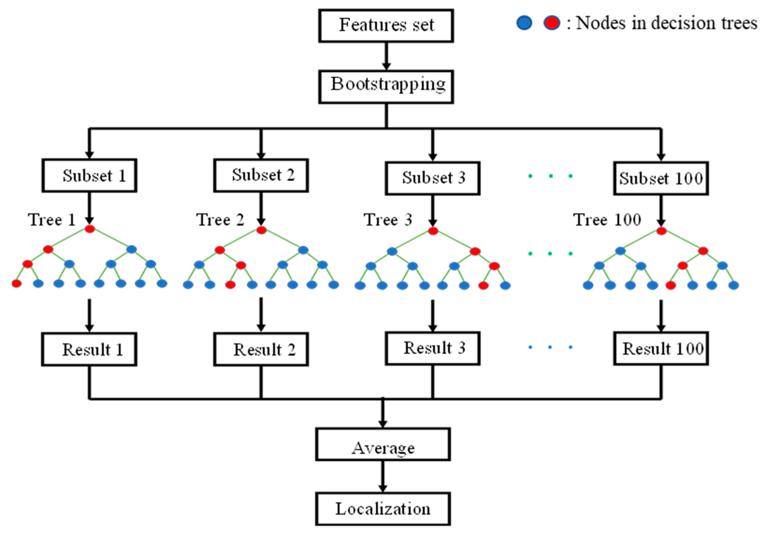
2.3. Impact Localization Using Random Forest
3. Experiment
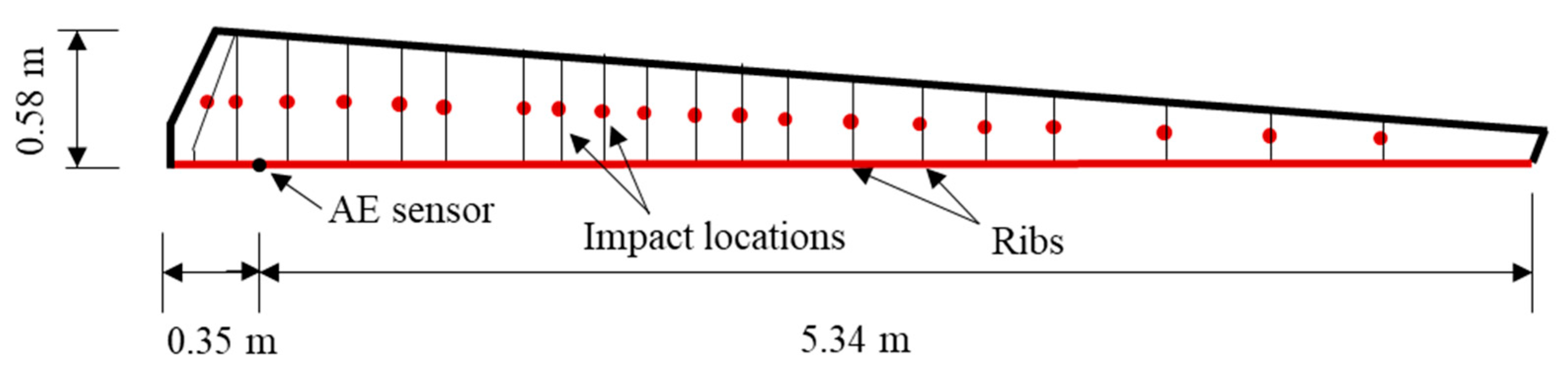
3.1. Specimen
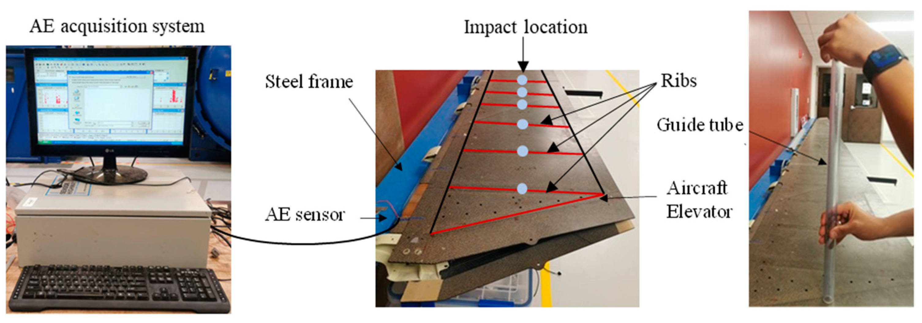
3.2. Impact Experiment Setup
3.3. Acoustic Emission Data Acquisition
4. Results and Discussion
4.1. Acoustic Emission Data Preprocessing
4.2. Localization Results Using Linear Regression
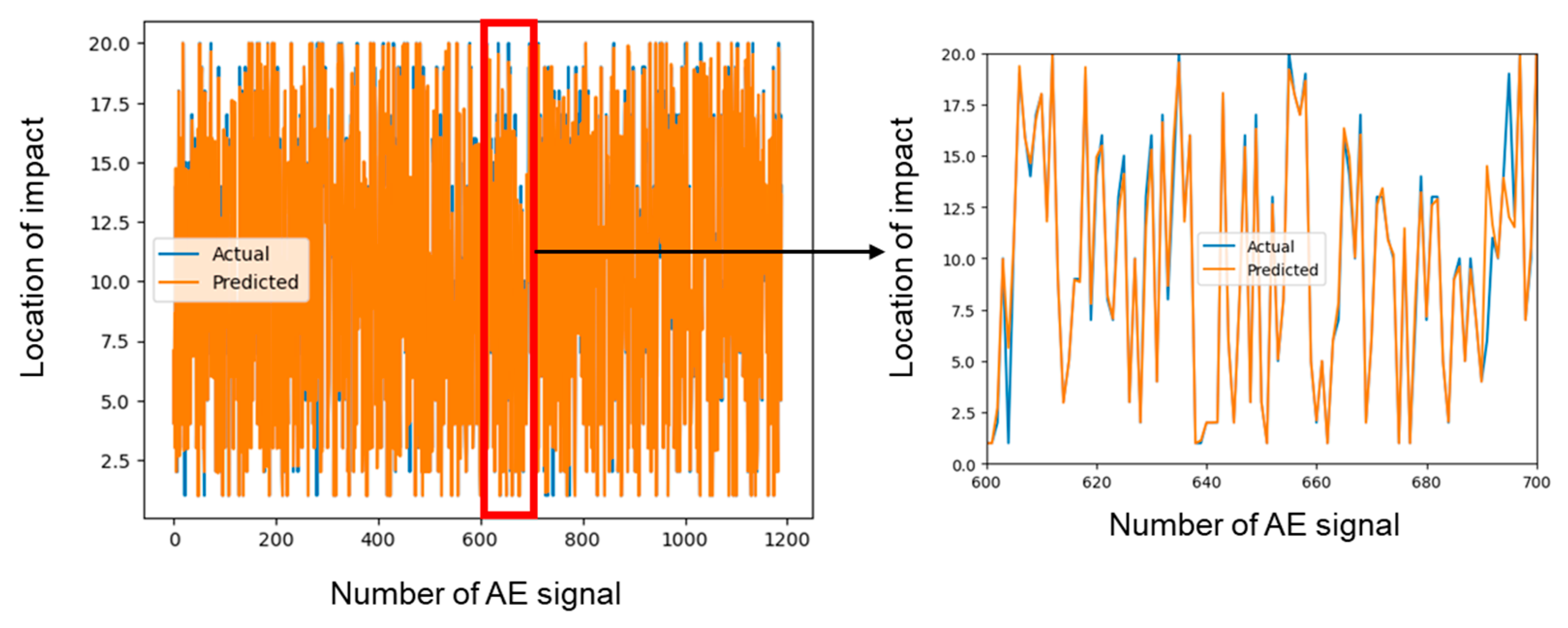
4.3. Localization Results Using Random Forest
5. Conclusions
- AE monitoring has the potential to be an effective tool for detecting and localizing impacts on aircraft elevators, offering a real-time and noninvasive monitoring solution for improved aircraft safety and maintenance.
- Both linear regression and random forest regression models demonstrated high accuracy in predicting impact locations, proving the effectiveness of regression algorithms in analyzing AE signals for impact localization.
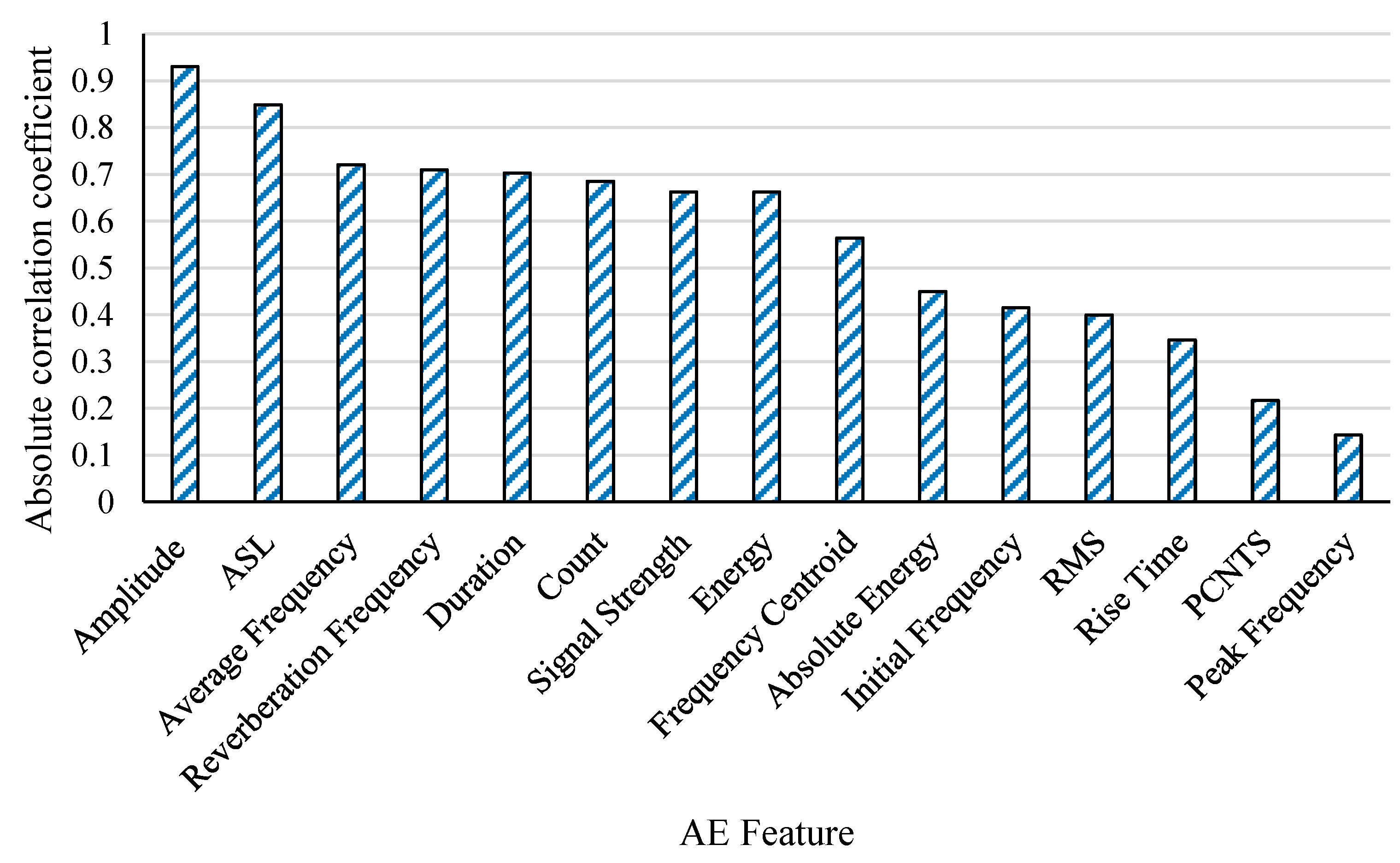
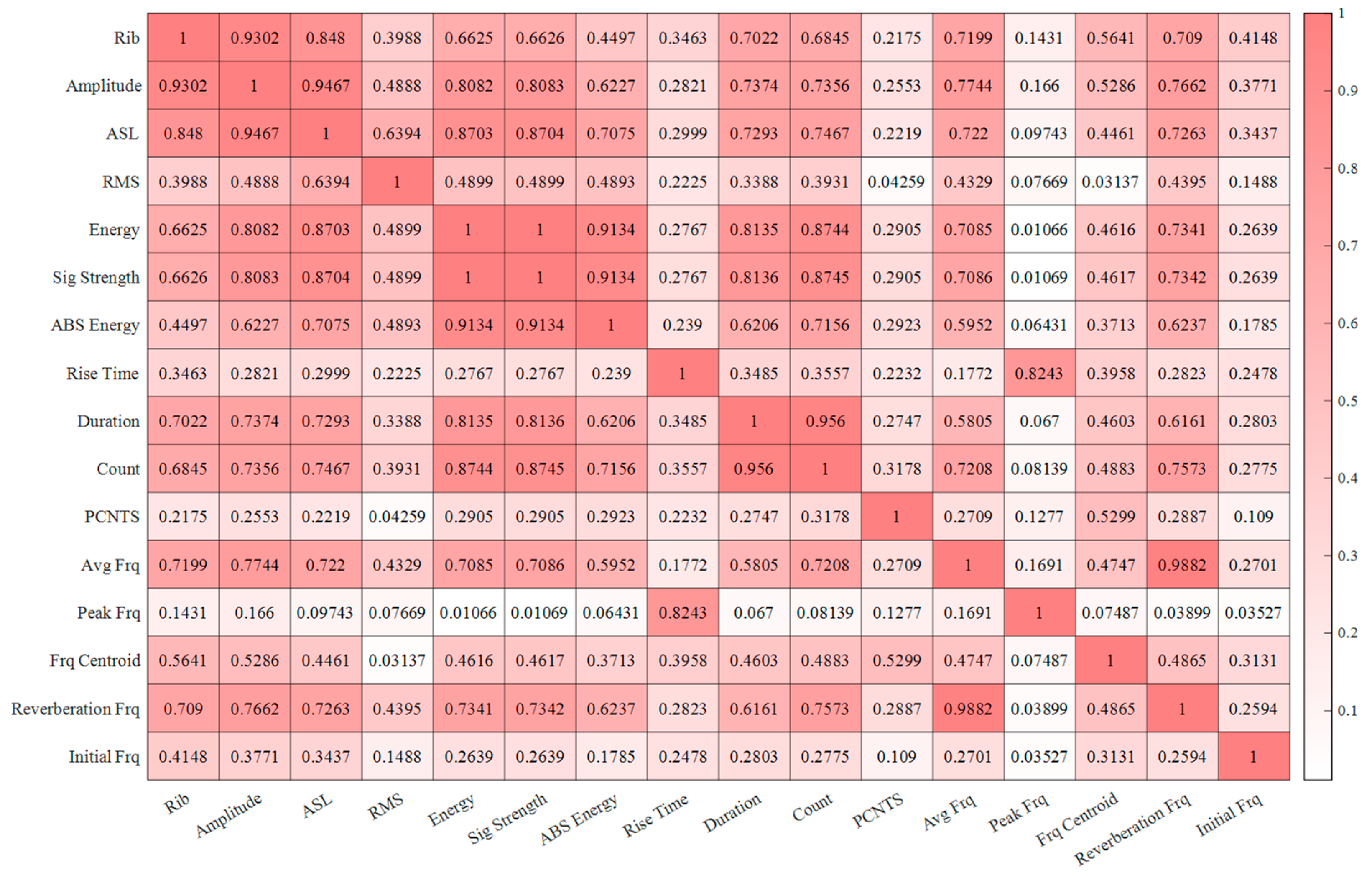
- The Pearson correlation analysis demonstrated a strong correlation between amplitude and impact location, suggesting that amplitude may be a critical factor in predicting the impact location using linear regression.
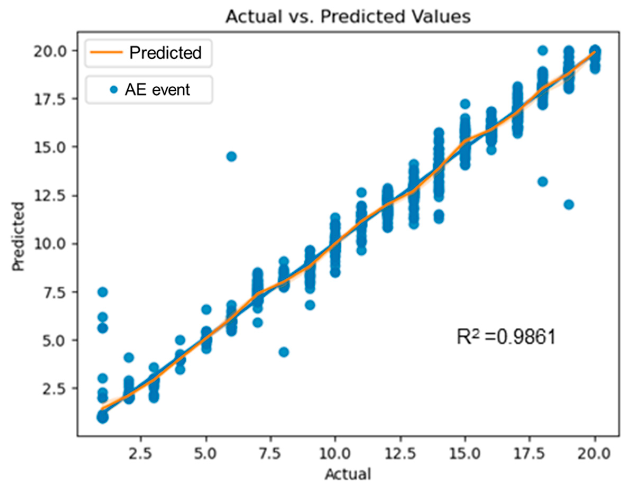
- The random forest model demonstrated better performance compared to the linear regression model, with a higher R2 value (0.98616) and a lower RMSE (0.6778), indicating its potential for practical applications in the aviation industry.
Author Contributions
Funding
Institutional Review Board Statement
Informed Consent Statement
Data Availability Statement
Conflicts of Interest
References
- Riccio, A.; Saputo, S.; Sellitto, A.; Lopresto, V. Characterization of the impact induced damage in composites by cross-comparison among experimental non-destructive evaluation techniques and numerical simulations. Proc. Inst. Mech. Eng. Part C J. Mech. Eng. Sci. 2017, 231, 3077–3090. [Google Scholar] [CrossRef]
- Habibi, M.; Laperrière, L.; Hassanabadi, H.M. Influence of low-velocity impact on residual tensile properties of nonwoven flax/epoxy composite. Compos. Struct. 2018, 186, 175–182. [Google Scholar] [CrossRef]
- Tian, Z.; Yu, L.; Leckey, C.; Seebo, J. Guided wave imaging for detection and evaluation of impact-induced delamination in composites. Smart Mater. Struct. 2015, 24, 105019. [Google Scholar] [CrossRef]
- Garrett, J.C.; Mei, H.; Giurgiutiu, V. An Artificial Intelligence Approach to Fatigue Crack Length Estimation from Acoustic Emission Waves in Thin Metallic Plates. Appl. Sci. 2022, 12, 1372. [Google Scholar] [CrossRef]
- Giannakeas, I.N.; Khodaei, Z.S.; Aliabadi, M. Digital clone testing platform for the assessment of SHM systems under uncertainty. Mech. Syst. Signal Process. 2022, 163, 108150. [Google Scholar] [CrossRef]
- Ai, L.; Zhang, B.; Ziehl, P. A transfer learning approach for acoustic emission zonal localization on steel plate-like structure using numerical simulation and unsupervised domain adaptation. Mech. Syst. Signal Process. 2023, 192, 110216. [Google Scholar] [CrossRef]
- Laxman, K.; Tabassum, N.; Ai, L.; Cole, C.; Ziehl, P. Automated crack detection and crack depth prediction for reinforced concrete structures using deep learning. Constr. Build. Mater. 2023, 370, 130709. [Google Scholar] [CrossRef]
- Tan, X.; Abu-Obeidah, A.; Bao, Y.; Nassif, H.; Nasreddine, W. Measurement and visualization of strains and cracks in CFRP post-tensioned fiber reinforced concrete beams using distributed fiber optic sensors. Autom. Constr. 2021, 124, 103604. [Google Scholar] [CrossRef]
- Tan, X.; Bao, Y. Measuring crack width using a distributed fiber optic sensor based on optical frequency domain reflectometry. Measurement 2021, 172, 108945. [Google Scholar] [CrossRef]
- Alvarez-Montoya, J.; Carvajal-Castrillón, A.; Sierra-Pérez, J. In-flight and wireless damage detection in a UAV composite wing using fiber optic sensors and strain field pattern recognition. Mech. Syst. Signal Process. 2020, 136, 106526. [Google Scholar] [CrossRef]
- Rocha, H.; Semprimoschnig, C.; Nunes, J.P. Sensors for process and structural health monitoring of aerospace composites: A review. Eng. Struct. 2021, 237, 112231. [Google Scholar] [CrossRef]
- Migot, A.; Mei, H.; Giurgiutiu, V. Numerical and experimental investigation of delaminations in a unidirectional composite plate using NDT and SHM techniques. J. Intell. Mater. Syst. Struct. 2021, 32, 1781–1799. [Google Scholar] [CrossRef]
- Salmanpour, M.S.; Khodaei, Z.S.; Aliabadi, M.H.F. Impact Damage Localization with Piezoelectric Sensors under Operational and Environmental Conditions. Sensors 2017, 17, 1178. [Google Scholar] [CrossRef]
- Ochôa, P.; Groves, R.M.; Benedictus, R. Systematic multiparameter design methodology for an ultrasonic health monitoring system for full-scale composite aircraft primary structures. Struct. Control. Health Monit. 2019, 26, e2340. [Google Scholar] [CrossRef]
- Ono, K. Application of acoustic emission for structure diagnosis. Diagnostyka 2011, 2, 3–18. [Google Scholar]
- Ono, K. Review on Structural Health Evaluation with Acoustic Emission. Appl. Sci. 2018, 8, 958. [Google Scholar] [CrossRef]
- Ai, L.; Soltangharaei, V.; Bayat, M.; Greer, B.; Ziehl, P. Source localization on large-scale canisters for used nuclear fuel storage using optimal number of acoustic emission sensors. Nucl. Eng. Des. 2021, 375, 111097. [Google Scholar] [CrossRef]
- Soltangharaei, V.; Anay, R.; Ai, L.; Giannini, E.R.; Zhu, J.; Ziehl, P. Temporal Evaluation of ASR Cracking in Concrete Specimens Using Acoustic Emission. J. Mater. Civ. Eng. 2020, 32, 04020285. [Google Scholar] [CrossRef]
- Laxman, K.C.; Ross, A.; Ai, L.; Henderson, A.; Elbatanouny, E.; Bayat, M.; Ziehl, P. Determination of vehicle loads on bridges by acoustic emission and an improved ensemble artificial neural network. Constr. Build. Mater. 2023, 364, 129844. [Google Scholar] [CrossRef]
- Ai, L.; Soltangharaei, V.; Ziehl, P. Developing a heterogeneous ensemble learning framework to evaluate Alkali-silica reaction damage in concrete using acoustic emission signals. Mech. Syst. Signal Process. 2022, 172, 108981. [Google Scholar] [CrossRef]
- Ono, K.; Gallego, A. Research and applications of AE on advanced composites. J. Acoust. Emiss 2012, 30, 180–229. [Google Scholar]
- Ai, L.; Soltangharaei, V.; Anay, R.; van Tooren, M.J.; Ziehl, P. Data-Driven Source Localization of Impact on Aircraft Control Surfaces. In Proceedings of the 2020 IEEE Aerospace Conference, Big Sky, MT, USA, 7–14 March 2020. [Google Scholar] [CrossRef]
- Barile, C.; Casavola, C.; Pappalettera, G.; Vimalathithan, P.K. Damage characterization in composite materials using acoustic emission signal-based and parameter-based data. Compos. Part B Eng. 2019, 178, 107469. [Google Scholar] [CrossRef]
- Xu, J.; Wang, W.; Han, Q.; Liu, X. Damage pattern recognition and damage evolution analysis of unidirectional CFRP tendons under tensile loading using acoustic emission technology. Compos. Struct. 2020, 238, 111948. [Google Scholar] [CrossRef]
- Mal, A.K.; Shih, F.; Banerjee, S. Acoustic emission waveforms in composite laminates under low velocity impact. In Proceedings of the NDE for health monitoring and diagnostics, San Diego, CA, USA, 2–6 March 2003. [Google Scholar] [CrossRef]
- James, R.; Joseph, R.P.; Giurgiutiu, V. Impact damage ascertainment in composite plates using in-situ acoustic emission signal signature identification. J. Compos. Sci. 2021, 5, 79. [Google Scholar] [CrossRef]
- Xu, J.; Liu, X.; Han, Q.; Wang, W. A particle swarm optimization–support vector machine hybrid system with acoustic emission on damage degree judgment of carbon fiber reinforced polymer cables. Struct. Health Monit. 2021, 20, 1551–1562. [Google Scholar] [CrossRef]
- Wang, Z.; Chegdani, F.; Yalamarti, N.; Takabi, B.; Tai, B.; El Mansori, M.; Bukkapatnam, S. Acoustic emission characterization of natural fiber reinforced plastic composite machining using a random forest machine learning model. J. Manuf. Sci. Eng. 2020, 142, 031003. [Google Scholar] [CrossRef]
- Ai, L.; Soltangharaei, V.; Bayat, M.; van Tooren, M.; Ziehl, P. Detection of impact on aircraft composite structure using machine learning techniques. Meas. Sci. Technol. 2021, 32, 084013. [Google Scholar] [CrossRef]
- Soltangharaei, V.; Ai, L.; Anay, R.; Bayat, M.; Ziehl, P. Implementation of Information Entropy, b-Value, and Regression Analyses for Temporal Evaluation of Acoustic Emission Data Recorded during ASR Cracking. Pract. Period. Struct. Des. Constr. 2021, 26, 04020065. [Google Scholar] [CrossRef]
- Ai, L.; Soltangharaei, V.; Ziehl, P. Evaluation of ASR in concrete using acoustic emission and deep learning. Nucl. Eng. Des. 2021, 380, 111328. [Google Scholar] [CrossRef]
- Unnþórsson, R. Hit detection and determination in AE bursts. Acoust. Emiss.-Res. Appl. 2013, 1–20. [Google Scholar]
- Su, X.; Yan, X.; Tsai, C.L. Linear regression. Wiley Interdiscip. Rev. Comput. Stat. 2012, 4, 275–294. [Google Scholar] [CrossRef]
- Uyanık, G.K.; Güler, N. A Study on Multiple Linear Regression Analysis. Procedia—Soc. Behav. Sci. 2013, 106, 234–240. [Google Scholar] [CrossRef]
- Maulud, D.; AbdulAzeez, A.M. A Review on Linear Regression Comprehensive in Machine Learning. J. Appl. Sci. Technol. Trends 2020, 1, 140–147. [Google Scholar] [CrossRef]
- Craven, B.; Islam, S.M. Ordinary least-squares regression. SAGE Dict. Quant. Manag. Res. 2011, 224–228. [Google Scholar]
- Breiman, L. Random forests. Mach. Learn. 2001, 45, 5–32. [Google Scholar] [CrossRef]
- Genuer, R.; Poggi, J.-M.; Tuleau-Malot, C. Variable selection using random forests. Pattern Recognit. Lett. 2010, 31, 2225–2236. [Google Scholar] [CrossRef]
- Ai, L.; Bayat, M.; Ziehl, P. Localizing damage on stainless steel structures using acoustic emission signals and weighted ensemble regression-based convolutional neural network. Measurement 2023, 211, 112659. [Google Scholar] [CrossRef]
- Van Ingen, J.W.; Buitenhuis, A.; Van Wijngaarden, M.; Simmons, F. Development of the Gulfstream G650 induction welded thermoplastic elevators and rudder. In Proceedings of the International SAMPE Symposium and Exhibition, Seattle, WA, USA, 23–28 May 2010. [Google Scholar]
- Allan, J.R. The costs of bird strikes and bird strike prevention. Hum. Confl. Wildl. Econ. Consid. 2000, 18. [Google Scholar]
- Nguyen, S.N.; Greenhalgh, E.S.; Graham, J.M.R.; Francis, A.; Olsson, R. Runway debris impact threat maps for transport aircraft. Aeronaut. J. 2014, 118, 229–266. [Google Scholar] [CrossRef]
- Greenhalgh, E.S.; Chichester, G.A.F.; Mew, A.; Slade, M.; Bowen, R. Characterization of the realistic impact threat from runway debris. Aeronaut. J. 2001, 105, 557–570. [Google Scholar] [CrossRef]
- Nguyen, S.N.; Greenhalgh, E.S.; Olsson, R.; Iannucci, L.; Curtis, P.T. Modeling the Lofting of Runway Debris by Aircraft Tires. J. Aircr. 2008, 45, 1701–1714. [Google Scholar] [CrossRef]
- Ebrahimkhanlou, A.; Dubuc, B.; Salamone, S. A generalizable deep learning framework for localizing and characterizing acoustic emission sources in riveted metallic panels. Mech. Syst. Signal Process. 2019, 130, 248–272. [Google Scholar] [CrossRef]
- Ebrahimkhanlou, A.; Dubuc, B.; Salamone, S. Damage localization in metallic plate structures using edge-reflected lamb waves. Smart Mater. Struct. 2016, 25, 085035. [Google Scholar] [CrossRef]


| Parametric Features | Feature Descriptions |
|---|---|
| Amplitude | The highest magnitude observed in the AE waveform. |
| Average signal level (ASL) | The effective voltage with a characteristic time TASL. |
| Root mean square (RMS) | The effective voltage with a characteristic time TRMS. |
| Energy | Quantification of the electrical energy contained within an AE signal. |
| Signal strength | The integral of the rectified voltage signal over the waveform duration. |
| Absolute energy | The absolute magnitude of electrical energy measured in an AE signal. |
| Rise time | The duration between the initial threshold crossing and the peak. |
| Duration | The time span encompassing the first and last threshold crossings. |
| Count | The count of instances where the signal crosses a predefined threshold. |
| Counts to peak (PCNTS) | The number of threshold crossings from the first crossing to the peak. |
| Average frequency | A parameter used to describe the overall frequency content of an AE signal. |
| Peak frequency | The frequency at which the signal exhibits its highest contribution. |
| Frequency centroid | A parameter used to characterize the overall frequency distribution or spectral content of an AE signal. |
| Reverberation frequency | The dominant frequency that persists after the initial, most intense portion of the signal has passed. |
| Initial frequency | The dominant frequency observed before the peak. |
| Coefficients of Variables | Delete None | Delete 1 | Delete 2 | Delete 3 | Delete 4 | Delete 5 | Delete 6 |
|---|---|---|---|---|---|---|---|
| Amplitude | −0.38874 | −0.40864 | −0.40198 | −0.43819 | −0.4686 | −0.47675 | −0.47685 |
| ASL | −0.14194 | −0.18554 | −0.1897 | −0.19827 | −0.10552 | −0.1097 | −0.11016 |
| Average Frequency | 0.054975 | −0.28685 | −0.30435 | −0.02979 | −0.02353 | −0.02833 | −0.02848 |
| Reverberation Frequency | −0.0445 | 0.28347 | 0.296833 | 0.035397 | 0.033767 | 0.042611 | 0.042782 |
| Duration | 1.56 × 10⁻⁵ | −6.00 × 10⁻⁶ | −2.00 × 10⁻⁵ | 1.37 × 10⁻⁵ | 1.48 × 10⁻⁵ | 2.34 × 10⁻⁵ | 2.31 × 10⁻⁵ |
| Count | −0.00236 | −0.00195 | −0.00168 | −0.00228 | −0.00215 | −0.00231 | −0.00232 |
| Signal Strength | −6.30 × 10⁻⁶ | −6.40 × 10⁻⁶ | −7.50 × 10⁻⁶ | −2.00 × 10⁻⁶ | −4.70 × 10⁻⁶ | −1.50 × 10⁻⁶ | −1.50 × 10⁻⁶ |
| Energy | −0.66253 | 0.054989 | 0.060861 | 0.02966 | 0.043758 | 0.024108 | 0.024254 |
| Frequency Centroid | −0.02227 | −0.03006 | −0.01738 | −0.03135 | −0.03521 | −0.03764 | −0.03763 |
| Absolute Energy | −2.30 × 10⁻⁶ | −9.00 × 10⁻⁷ | −3.50 × 10⁻⁷ | −1.10 × 10⁻⁶ | 8.92 × 10⁻⁸ | 5.72 × 10⁻⁸ | / |
| Initial Frequency | 0.000384 | −0.00117 | −0.0014 | −0.00319 | −0.00323 | / | / |
| RMS | 33.16985 | 65.97887 | 66.95417 | 50.09611 | / | / | / |
| Rise Time | 0.00504 | 0.001808 | 0.001882 | / | / | / | / |
| PCNTS | 0.010839 | 0.014069 | / | / | / | / | / |
| Peak Frequency | −0.05168 | / | / | / | / | / | / |
| Intercept | 36.09853 | 39.63695 | 39.70405 | 43.43703 | 43.1448 | 43.42157 | 43.43426 |
| R2 | 0.9361 | 0.9281 | 0.9255 | 0.9197 | 0.9187 | 0.9176 | 0.9176 |
| RMSE | 1.4614 | 1.5507 | 1.5784 | 1.6390 | 1.6485 | 1.6599 | 1.6599 |
| Coefficients of Variables | Delete 7 | Delete 8 | Delete 9 | Delete 10 | Delete 11 | Delete 12 | Delete 13 |
|---|---|---|---|---|---|---|---|
| Amplitude | −0.53962 | −0.53972 | −0.54393 | −0.58384 | −0.60369 | −0.60258 | −0.59833 |
| ASL | −0.04556 | −0.04548 | 0.201282 | 0.235985 | 0.230852 | 0.229102 | 0.228328 |
| Average Frequency | 0.002124 | 0.002091 | −0.0418 | −0.03239 | 0.012376 | 0.004003 | / |
| Reverberation Frequency | 0.019079 | 0.019156 | 0.017189 | 0.037602 | −0.00845 | / | / |
| Duration | 5.61 × 10⁻⁵ | 5.63 × 10⁻⁵ | −0.00013 | −3.50 × 10⁻⁵ | / | / | / |
| Count | −0.00284 | −0.00284 | 0.001274 | / | / | / | / |
| Signal Strength | −4.50 × 10⁻⁶ | 2.37 × 10⁻⁶ | / | / | / | / | / |
| Energy | 0.042939 | / | / | / | / | / | / |
| Frequency Centroid | / | / | / | / | / | / | / |
| Absolute Energy | / | / | / | / | / | / | / |
| Initial Frequency | / | / | / | / | / | / | / |
| RMS | / | / | / | / | / | / | / |
| Rise Time | / | / | / | / | / | / | / |
| PCNTS | / | / | / | / | / | / | / |
| Peak Frequency | / | / | / | / | / | / | / |
| Intercept | −0.53962 | −0.53972 | −0.54393 | −0.58384 | −0.60369 | −0.60258 | −0.59833 |
| R2 | 0.9115 | 0.9115 | 0.8784 | 0.8774 | 0.8757 | 0.8757 | 0.8757 |
| RMSE | 1.7198 | 1.7199 | 2.0162 | 2.0247 | 2.0386 | 2.0387 | 2.0390 |
Disclaimer/Publisher’s Note: The statements, opinions and data contained in all publications are solely those of the individual author(s) and contributor(s) and not of MDPI and/or the editor(s). MDPI and/or the editor(s) disclaim responsibility for any injury to people or property resulting from any ideas, methods, instructions or products referred to in the content. |
© 2023 by the authors. Licensee MDPI, Basel, Switzerland. This article is an open access article distributed under the terms and conditions of the Creative Commons Attribution (CC BY) license (https://creativecommons.org/licenses/by/4.0/).
Share and Cite
Ai, L.; Flowers, S.; Mesaric, T.; Henderson, B.; Houck, S.; Ziehl, P. Acoustic Emission-Based Detection of Impacts on Thermoplastic Aircraft Control Surfaces: A Preliminary Study. Appl. Sci. 2023, 13, 6573. https://doi.org/10.3390/app13116573
Ai L, Flowers S, Mesaric T, Henderson B, Houck S, Ziehl P. Acoustic Emission-Based Detection of Impacts on Thermoplastic Aircraft Control Surfaces: A Preliminary Study. Applied Sciences. 2023; 13(11):6573. https://doi.org/10.3390/app13116573
Chicago/Turabian StyleAi, Li, Sydney Flowers, Tanner Mesaric, Bryson Henderson, Sydney Houck, and Paul Ziehl. 2023. "Acoustic Emission-Based Detection of Impacts on Thermoplastic Aircraft Control Surfaces: A Preliminary Study" Applied Sciences 13, no. 11: 6573. https://doi.org/10.3390/app13116573