
A Spectral Method Algorithm for Modeling the Dispersion of Non-Axisymmetric Modes in Fluid-Filled Elastic Tubes

1
National Key Laboratory of Underwater Acoustic Technology, Harbin Engineering University, Harbin 150001, China
2
Key Laboratory of Marine Information Acquisition and Security (Harbin Engineering University), Ministry of Industry and Information Technology, Harbin 150001, China
3
College of Underwater Acoustic Engineering, Harbin Engineering University, Harbin 150001, China
*
Author to whom correspondence should be addressed.
Appl. Sci. 2023, 13(22), 12415; https://doi.org/10.3390/app132212415
Submission received: 17 October 2023
/
Revised: 9 November 2023
/
Accepted: 14 November 2023
/
Published: 16 November 2023
(This article belongs to the Special Issue Acoustics and Vibrations Analyses of Materials at Different Scales: Experimental and Numerical Approaches: Volume III)
Abstract
:In order to design a low-noise water-filled pipeline system, it is necessary to obtain knowledge of the dispersion characteristics of axial propagation modes in different water-filled elastic tubes. In this work, an algorithm is developed based on the spectral method, which has previously been used to solve the dispersion of axisymmetric modes in cylindrical structures but has not yet been applied to non-axisymmetric modes. The algorithm can obtain the dispersion characteristics, modal displacement, and stress distribution of axial propagation modes in a fluid-filled elastic multi-layer tube. The algorithm behaves well both at low and ultrasonic frequencies, and it is suitable for any tube dimensions, wall thickness and layers. The results of a water-filled PMMA tube obtained using the spectral method algorithm were verified using a COMSOL simulation, while the dispersion curves of the same tube from the literature were found to be missing some low-order modes. In addition, the dispersion curves of a water-filled three-layer tube are given. The spectral method algorithm has the advantages of fast calculation speed, less computational resources consumed, accurate results, and no modal omission.
1. Introduction
Fluid-filled pipeline systems are widely used in engineering. Pumps, valves, and other pipeline system components often vibrate during operation. Vibrational energy propagates in the fluid and pipe walls in the form of waves, producing a negative effect on the system performance and the surrounding environment. Axially propagating waves contain axisymmetric and non-axisymmetric modes related to frequencies. The accurate and efficient calculation of dispersion curves of theses modes and the corresponding displacement and stress distribution is a key step in studying the dispersion characteristics of propagation modes in a fluid-filled elastic tube, which lays a theoretical foundation for the subsequent design of low-noise pipeline systems and non-destructive pipeline testing tools.
A great deal of research has been carried out on the dispersion characteristics of axially propagating modes in hollow cylindrical shells and fluid-filled tubes. Jacobi [1] took the ideal liquid cylinder as a research object and obtained the dispersion curves of low-frequency axisymmetric modes under various non-dissipative boundary conditions: rigid walls, pressure-release walls, an infinite liquid boundary, liquid walls, and thin solid walls. In order to study propagation modes over a wider frequency range, Lin and Morgan [2] used the approximate equations governing the motion of an elastic tube wall to derive the characteristic equation of the modes. Gazis [3,4] described the motion of cylindrical shells using the linear elastic theory proposed by Pochhammer [5] and Chree [6] and obtained the eigenmode characteristic equation of an infinitely long isotropic hollow cylinder. Del Grosso [7] calculated the dispersion relation of axially propagating modes in liquid-filled tubes with arbitrary wall thicknesses based on the exact longitudinal and transverse wave equations. Kumar [8] obtained the dispersion equation of axially propagating modes in a liquid-filled cylindrical shell using the exact three-dimensional linear elastic equation and the fluid motion equation and discussed the characteristics of the bending mode (). Using the theory of Del Grosso [7], Lafleur and Shields [9] calculated the dispersion relation of axisymmetric propagating modes in a water-filled elastic tube. Using linear elasticity and classical perfect slip boundary conditions at the solid–fluid boundary, Sinha et al. [10,11] analyzed the behavior of axisymmetric longitudinal waves in cylindrical shells with different internal and external fluids and also carried out an experimental verification. Easwaran and Munjal [12] used the same method to study the lowest-order acoustic modes in a liquid-filled impedance tube. Greenspon and Singer [13] replaced the elastic constants in the three-dimensional elastic equation with complex viscoelastic material parameters and studied the axisymmetric modes and non-axisymmetric modes in a liquid-filled viscoelastic tube. Berliner and Solecki [14,15] also derived the dispersion equation of wave propagation in a transversely isotropic elastic tube from the three-dimensional elastic equation and discussed the dispersion characteristics of the non-axisymmetric mode . Baik [16] applied Del Grosso’s [7] theory to viscous liquids to predict the decay of axisymmetric modes in liquid-filled tubes.
The common aspect of the above research is that the modal dispersion characteristics were obtained by the so-called “root-finding method”. As for a multi-layer wave guide, the traditional ways of constructing system matrices are the transfer matrix [17,18] technique and the global matrix [19] technique. When the thickness of the multi-layer model is large or the solving frequencies are high, the transfer matrix technique is prone to numerical instability [20], and although the global matrix technique does not have this problem, its matrix size becomes larger as the number of model layers increases, and the solving process of the characteristic equation becomes extremely slow.
The spectral method has been widely used in fluid dynamics since the 1970s [21,22], but it was not until 2004 that it was first introduced to acoustic engineering by Adamou [23] for solving the dispersion equation of modes in elastic waveguide structures. Research has shown that the spectral method is easier to implement in a numerical program than the traditional root-finding method, provides faster calculation speeds, and is more suitable for dealing with curving, damping, and inhomogeneous and anisotropic model problems. Using the spectral method, Karpfinger et al. [24,25] developed a set of algorithms for solving the dispersion characteristics of axisymmetric modes in multi-layer cylindrical structures.
To date, there has been no research on the dispersion characteristics of non-axisymmetric modes in fluid-filled elastic tubes using the spectral method. In this paper, a new algorithm based on the spectral method is proposed, which obtains the dispersion curves of the axial propagation modes in fluid-filled elastic tubes. It can also calculate the displacement distribution and stress distribution of the axial propagation modes in the radial direction. The algorithm proposed here works well in spite of tube dimensions, wall thickness, layers and frequency ranges. The results of the algorithm are verified using a COMSOL simulation. We found that there existed some modes omission of the dispersion curves presented in the literature [26].
2. Theory
2.1. Wave Equations
In this section, using linear elastic theory, the governing wave propagation equations in the elastic tube wall and the fluid are derived, respectively. The corresponding boundary conditions at different interfaces are given.
Figure 1 shows an infinite, homogeneous, and isotropic fluid-filled elastic tube model. The inner radius of the tube is , the outer radius is , and the cylindrical coordinate system is established with the axis of the cylindrical tube as the z-axis. Waves propagating along the axial direction in a fluid-filled elastic tube can be divided into longitudinal waves and torsional waves, both of which have axisymmetric modes and non-axisymmetric modes [27]. In some references, longitudinal and torsional waves are defined as waves with only axisymmetric modes, and waves with non-axisymmetric modes are collectively called flexural waves. In this paper, the positive integer is used to represent the circumferential order of the mode, and the axisymmetric mode satisfies .
For the elastic tube model in Figure 1, assuming that the outer surface satisfies the stress-free boundary condition, the wave equation governing the propagation of elastic waves [27] is
where represents the displacement field, which is a function of the three cylindrical coordinates and time. The bulk wave velocities in the elastic material are determined by the density and the Lamé constants and . If represents the dilatational longitudinal bulk wave velocity and is the shear bulk wave velocity, then
The displacement field can be described using the dilatational scalar potential and the equivoluminal vector potential :
Substituting Equation (4) into Equation (1) gives
Using elasticity theory, the potentials and have the following form in cylindrical coordinates:
Gazis [3] presented expressions for the potentials satisfying Equations (5) and (6):
where the integer is known as the circumferential order of a wave mode and is the axial wavenumber. , , , and are unknown functions related only to .
Let
Substituting Equation (9) into Equations (5) and (6), and dropping , after a series of mathematical transformations, the equation of a wave propagating in an infinitely long, homogeneous, and isotropic elastic tube wall can be obtained as
The wave equation in the fluid is
where the subscript represents the fluid and is the sound velocity of the fluid in the tube.
The displacement potential function is
Substituting Equation (13) into Equation (12), the equation of an acoustic wave propagating in the fluid is obtained as
2.2. Boundary Conditions
In order to obtain the dispersion equation of axial propagation modes in a fluid-filled elastic tube, it is necessary to set reasonable boundary conditions.
If the elastic tube wall is composed of multi-layer materials, at the solid 1–solid 2 interface, the continuous condition to be satisfied is that the displacement components , , and the surface stress components , , in the solid 1 are equal to the corresponding components in the solid 2, as shown in Equation (15). Subscripts and represent the solid 1 and the solid 2, respectively, and represents the interface.
For the solid–fluid interface, if the viscosity of the fluid cannot be ignored, the continuous condition at the interface is that the displacement components and the surface stress components in the solid are equal to the corresponding components in the viscous fluid, as shown in Equation (16). Subscripts and represent the solid and the viscous fluid, respectively.
If the viscosity of the fluid is negligible, the boundary condition at the interface is a perfect slip boundary condition. That is, the radial component of the displacement of the solid and the fluid are equal, the circumferential component and the axial component of the displacement are discontinuous, and the surface stress components are still equal. The shear stress of the non-viscous fluid does not exist, that is, , as shown in Equation (17):
The outer tube wall satisfies the stress-free boundary condition, as shown in Equation (18). The subscript represents the tube wall and represents the outer tube wall.
In addition, for an infinitely long tube, the inner and outer wall of the tube should meet:
The above Equations (15)–(19) constitute the boundary conditions that a fluid-filled elastic tube needs to be satisfied under different conditions. Expressions for these physical quantities in the above boundary conditions are given below.
2.2.1. Physical Quantities in the Tube Wall
Substituting Equation (9) into Equations (20)–(22) and using to represent accruing to Equation (10), yields the displacement field:
where
The stress tensor components in the elastic tube wall can be obtained using the following equations [27]:
Substituting Equations (23)–(25) into equations for , , and , one obtains the stress field:
In addition, in the cylindrical coordinate system,
Using , , to represent , one obtains
2.2.2. Physical Quantities in the Fluid
The displacement components of the non-viscous fluid are expressed as
The stress tensor components of the inviscid fluid are
The wave equations in Equation (11), Equation (14), and the boundary conditions in Equations (15)–(19) constitute an eigenvalue problem. The traditional root-finding method is to select the appropriate general solution form of the wave equations, and to substitute the general solution into the appropriate boundary conditions to obtain a set of uniform linear geometric equations. The determinant of the coefficient matrix is set equal to zero, and the so-called dispersion equation is obtained. Finally, the root of the dispersion equation is found using numerical methods, and the dispersion relationship of modes is obtained.
The general solution of the wave equations in the cylindrical coordinate system contains various forms of Bessel functions, and it is often difficult to separate and determine the root of different modes. If factors such as fluid viscosity and solid loss need to be considered, the dispersion equation becomes more difficult to solve. The spectral method introduced in the next section can help effectively avoid these problems.
3. The Spectral Method Algorithm for a Fluid-Filled Elastic Tube
3.1. The Spectral Method Theory
The advantage of the spectral method is that it does not require calculation of the root of the Bessel functions, but instead uses the differential matrix to solve the eigenvalue problem. The core idea is to approximate unknown functions to be solved in the differential equation through global interpolation using high-order orthogonal polynomials. As for the eigenvalue problem of a fluid-filled elastic tube, the differentiation occurs on a bounded interval, ; the appropriate choice is to use Chebyshev polynomials to construct the differential matrix according to Boyd [28]. The choice of polynomials for different unknown function is listed in Appendix A, Table A1.
The differential matrix is defined as follows according to Adamou [23]:
where is the value of the function evaluated at the interpolation point , , is the th derivative of , and the matrix is the differential matrix.
The MATLAB program chebdif [29] generates interpolation points on the interval :
Here, interpolation points for are
where denotes the outer radius, denotes the inner radius.
generated by chebdif [29] approximates , but here requires the approximation of , which is given by
Wave equations and boundary conditions only deal with derivatives, so the spectral method algorithm in the next section uses to represent for simplicity.
Adamou [23] gave a heuristic argument about the theoretical accuracy of the spectral method. For on the Chebshev interval , it requires at least two interpolation points per wavelength to accurately resolve . If is large enough, the interpoint spacing is asymptotically according to Equation (41). Assuming the wavelength of is , and it is roughly constant across the domain, then the condition for accurate resolution is
A more formal demonstration based on the convergence rates of Chebyshev series can be found in the study of Gottlieb and Orszag [30].
3.2. The Spectral Method Algorithm
Wave equations and the corresponding boundary conditions in Section 2 are expressed in terms of the differential matrix as follows.
The wave Equation (11) in the elastic tube wall can be written as
where is a differential matrix and expressions for are
In Equations (46)–(49), denotes a diagonal matrix and denotes an unit matrix.
The wave Equation (14) in the fluid is expressed in the form of the differential matrix as
Thus, the differential matrix expression of equations for wave propagation in a fluid-filled elastic tube is as follows:
Similarly, the differential matrix expressions for the displacement vector components in the elastic pipe wall are
The corresponding coefficients are
The differential matrix expressions for the stress tensor components in the elastic tube wall are
The corresponding coefficients are
The differential matrix expression of Equation (34) is
The coefficients can be given as
For the fluid, the differential matrix expressions of the displacement vector components are as follows:
The differential matrix expression of the stress tensor component of the fluid is
Taking the fluid-filled elastic tube with a single-layer wall as an example, Figure 2 shows the appropriate position of the boundary conditions in the matrix.
This can be performed by introducing a matrix on the right-hand side of Equation (51), as shown in Equation (68):
where is a matrix consisting of potential functions:
is a matrix and can be defined as follows:
where is an diagonal matrix with the following form:
Equation (68) is a generalized eigenvalue problem that can be solved using the MATLAB routine [24].
By changing the value of the frequency , a different dispersion relation can be obtained from Equation (68). For a given relationship between , the dispersion curves of the modes can be drawn. At the same time, the potential functions in Equation (69) are substituted into Equation (52), Equation (56), Equation (62), and Equation (66), which are the displacement vector components and stress tensor components of the modes in the tube wall and in the fluid. One can then obtain the displacement and stress distribution of the axial propagation modes in the fluid-filled tube with frequency with respect to the radial direction.
The flowchart of the proposed spectral method algorithm is shown in Figure 3.
4. Discussion
In this section, the dispersion characteristics of axial propagation modes in a water-filled PMMA tube, whose parameters are from Baik [26], were calculated using the algorithm described in Section 3. The results of the algorithm were verified using a COMSOL simulation. In addition, differences between dispersion curves obtained from the algorithm and Baik [26] were analyzed. Finally, the dispersion curves of a water-filled multi-layer tube were given.
4.1. Comparison between the Spectral Method Algorithm and the COMSOL Simulation
The parameters of the water-filled PMMA tube adopted by Baik [26] are shown in Table 1, where is the inner radius of the tube, is the wall thickness, , are the longitudinal and shear sound speed of PMMA, respectively, is the sound speed in water, is the density of PMMA, and is the density of water.
The two-dimensional model of the water-filled PMMA tube with the above parameters was established in COMSOL, as shown in Figure 4.
The inner part was water, and its physical field was set to be a “Pressure Acoustics” field. The wave equation for time-harmonic acoustic waves in 2D geometry is Equation (72),
Where means total pressure, which is the sum of and the possible background pressure field , as shown in Equation (74):
is shown as Equation (75), where is the out-of-plane wave number:
The subscript “c” in and means that they may be complex-valued. Lossy media, like porous materials or highly viscous fluids, can be modeled by using the complex-valued speed of sound and density.
In Equation (72), is the dipole domain source, which corresponds to a domain force source on the right-hand side of the momentum equation, and is the monopole domain source, which corresponds to a mass source on the right-hand side of the continuity equation.
In the mode analysis study of COMSOL, is used as the eigenvalue.
The outer part is the PMMA tube wall, and its physical field, is set to be a “Solid Mechanics” field. The governing equation used here is
In Equation (76), is the structural displacement vector, and is the elasticity tensor.
The outer tube wall is the free boundary, which satisfies the stress-free boundary condition, and the inner tube wall is set to be the “Acoustic-Structure Boundary”, which is used to couple a Pressure Acoustics model to any structural component. The coupling includes the fluid load on the structure and the structural acceleration as experienced by the fluid.
The condition on exterior boundaries is shown as Equations (77) and (78):
where is the structural acceleration, is the surface normal, is the total acoustic pressure and is the load (force per unit area) experienced by the structure.
The condition on interior boundaries is shown as follows:
such that the acoustic load is given by the pressure drop across the thin structure. The up and down subscripts refer to the two sides of the interior boundary.
In order to find out the influence of mesh grids on the COMSOL simulation results, five different meshes were used to calculate the mode wavenumber, as shown in Table 2.
The wave number of the axial propagation modes in the water-filled PMMA tube at kHz was calculated using COMSOL with five different mesh files, as shown in in Table 2. The differences in at each mode between mesh 1–4 and mesh 5 are plotted in Figure 5. The horizontal axis is the mode index, meaning that there exist 22 modes at kHz. The vertical axis is the absolute value of the difference between mesh 1–4 and mesh 5 at each mode. Figure 5 shows that the simulation result of each mode tends to be consistent with the increase in the number of grid elements. In order to achieve the most accurate calculation results, the following simulation used mesh 5.
The mode analysis in COMSOL can calculate the wave number and mode shape of a propagation mode at a specific frequency. Combined with sweep analysis, dispersion curves of the axial propagation mode of the water-filled PMMA tube can be obtained. The frequency range calculated here is 0–90 kHz and the frequency interval is 200 Hz.
Figure 6 shows the comparison of the dispersion curves obtained from the COMSOL simulation and the spectral method algorithm.
In Figure 6, the horizontal axis is the dimensionless parameter , as shown in Equation (82), and the vertical axis is the normalized phase velocity . The vertical axis uses logarithmic coordinates.
The curves in Figure 6 represent the calculation results from the spectral method algorithm and the dots represent the COMSOL simulation results. It can be seen from Figure 6 that the dispersion curves of the axial propagation modes in the water-filled PMMA tube obtained from the spectral method algorithm were completely consistent with the COMSOL simulation results.
Table 3 shows the time consumed by the COMSOL Multiphysics 5.6 software and the spectral method algorithm implemented in MATLAB R2022b to obtain the dispersion curves in Figure 6. The computer used here to run the COMSOL simulation and the MATLAB program of the proposed algorithm was a Lenovo desktop workstation, which has 2 Intel® Xeon® Silver 4110 CPU, and 128 GB RAM. The spectral method algorithm not only provides an accurate calculation but requires much less time and CPU resources to do so than the COMSOL simulation software.
Table 4 compares the wavenumbers of the axial propagation modes in the water-filled PMMA tube at kHz provided by the COMSOL simulation and the spectral method algorithm. The error in the table was calculated using Equation (83), where represents the axial wavenumber calculated using the spectral method and represents the axial wavenumber calculated using the COMSOL simulation.
It can be seen from Table 4 that both the COMSOL simulation and the spectral method algorithm can find 12 different modes at 8 kHz, and the axial wavenumber corresponding to the same mode is identical under two different calculation ways.
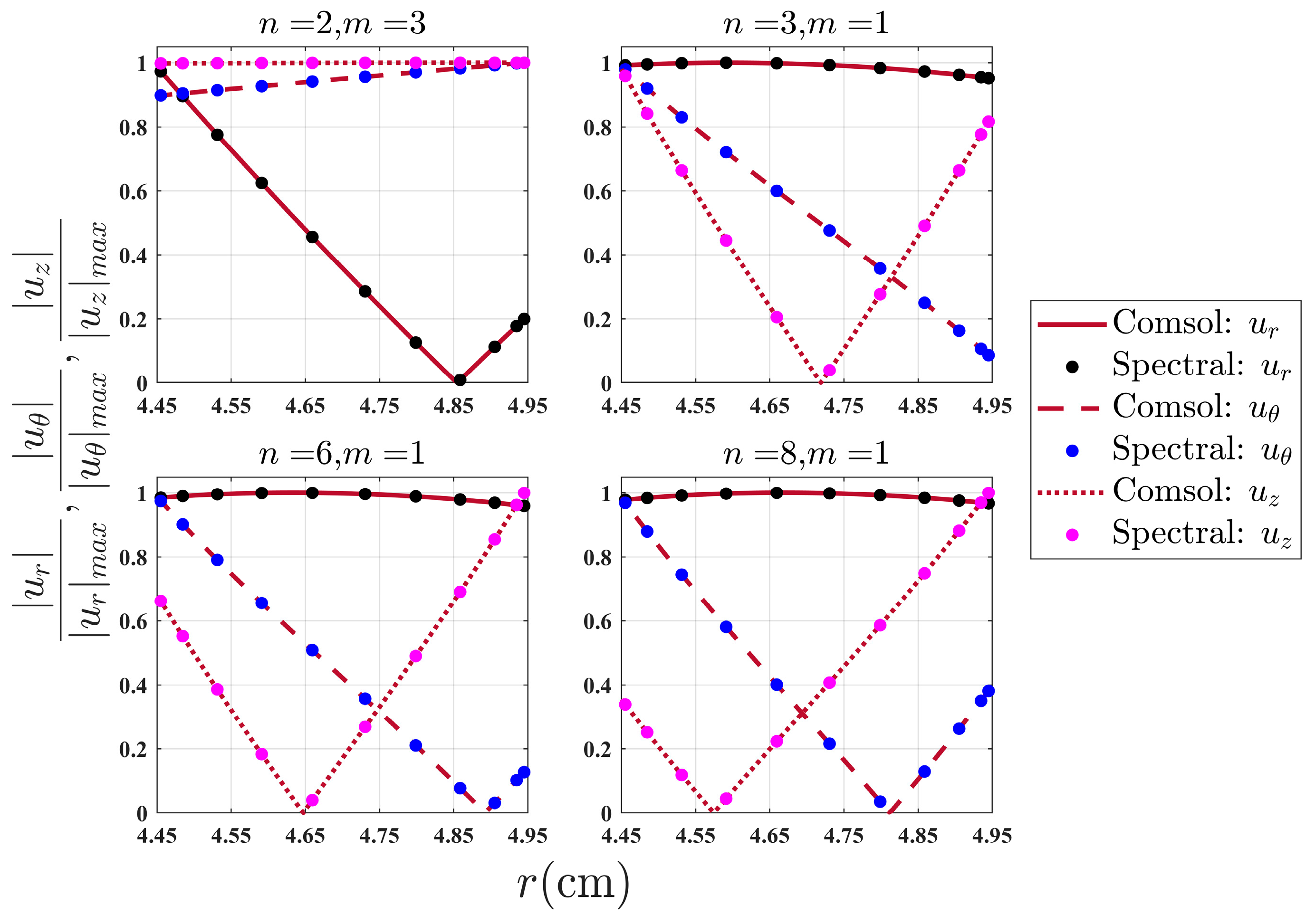
Figure 7 shows the radial distribution of the displacement components , , of some non-axisymmetric modes in the tube wall at kHz. The modes are indexed as , where is the circumferential order. The transverse axis represents the radial component in cylindrical coordinates, and the longitudinal axis is the normalized value of each displacement component. It can be seen from the figure that the distribution of the displacement components of the non-axisymmetric modes () in the tube wall obtained by the spectral method algorithm was consistent with the COMSOL simulation results.
In conclusion, the dispersion curves of axial propagation modes in the water-filled tube obtained using the spectral method algorithm are consistent with the results from the COMSOL simulation. In addition, the algorithm can find all the axial propagation modes at any frequency correctly, and obtain the precise mode displacement distribution in the tube wall. The spectral method algorithm consumes much less time and computation resources to acquire such results.
4.2. Differences between the Results from the Spectral Method Algorithm and Baik [26]
Figure 8 shows the phase velocity curves of the axisymmetric modes () and the non-axisymmetric modes () of a water-filled PMMA tube propagating along the axis, as obtained from the spectral method algorithm. Figure 9 shows the group velocity curves of the corresponding modes. In the graphs, the horizontal axis is the dimensionless parameter and the vertical axis is the phase velocity or group velocity normalized by the sound velocity in water as or . All figures use to represent the circumferential order of the modes. The different color of lines in Figure 8 and Figure 9 denote a different group number of the modes with the same . Figure 8 and Figure 9 are compared with Figure 2 in Baik [26], which shows the dispersion curves of phase speed and group speed of modes for the water-filled PMMA tube obtained.
Table 5 shows the modal correspondence between the dispersion curves obtained using the spectral method algorithm and results from Baik [26]. For example, the mode in Figure 8 corresponds to the mode in Figure 2 of Baik [26], et cetera. This work only analyzed the modes listed in Table 5. The following analysis was based on the mode indices in Figure 8.
For the axisymmetric modes (), Baik [26] did not find the mode in Figure 8, obtained with the spectral method algorithm. For the non-axisymmetric modes (), Baik [26] lacked the modes , , , , , in Figure 8. The accuracy of the spectral method algorithm was verified using the results from the COMSOL simulation in the previous section.
It can be seen from Figure 8 that the phase velocity of mode did not change with the frequency, and was equal to the bulk shear wave velocity of the PMMA tube. Its group velocity was also equal to the bulk shear wave velocity, as shown in Figure 9. This is consistent with the description of the dispersion characteristics of the torsional wave provided by Gazis [3].
The phase velocities of modes , , , and in Figure 8 were lower than the sound velocity in water, and the longitudinal and shear bulk wave velocities of the PMMA tube. Figure 10 and Figure 11 show the radial distribution of the displacement components and the stress tensor components of the above four modes at kHz, obtained using the spectral method algorithm.
In Figure 10, the solid line represents , the dotted line represents , and the dashed line represents . In Figure 11, the solid line represents , the dotted line represents , and the dashed line represents . It can be seen from Figure 10 that the maximum amplitude of the axial displacement component of these four modes in the water was larger than that in the tube wall, and the energy carried in the water was higher than that in the tube wall. These phenomena are similar to a Scholte wave propagating at the solid–fluid interface. Baik [26] only obtained the mode, which is labeled as the mode in Figure 10.
The modes , , and in Figure 8 are flexural waves propagating along the axial direction.
In conclusion, dispersion curves of the water-filled PMMA tube provided by Baik [26] missed the torsional wave mode , Scholte wave modes , , and , and flexural wave modes , , and . In contrast, the spectral method algorithm can find all the axial propagation modes precisely without missing any low-order modes.
4.3. A Water-Filled Elastic Multi-Layer Tube Model
The calculation model used in the above has only one layer in the tube wall. Here, the spectral method algorithm was used to obtain the dispersion curves of a water-filled multi-layer elastic tube. The cross section of the tube is shown in Figure 12. The materials of Layer 1, Layer 2 and Layer 3 were PVC, iron and PVC, respectively.
The parameters of the tube are shown in Table 6, where is the inner radius of the tube, , , are thickness of Layer 1, Layer 2 and Layer 3, respectively, , are the longitudinal and shear sound speed of the solid material, respectively, is the density of the solid material, m/s is the sound speed in water, and kg/m3 is the density of water.
The phase velocity curves of the water-filled multi-layer elastic tube are shown in Figure 13; the horizontal axis is the frequency (kHz) and the vertical axis is . The frequency range in Figure 13 is 0–2 kHz. In Figure 13, the axial propagation modes are plotted in different subgraphs according to the circumferential order . It shows that the spectral method algorithm worked well for the large-dimension, thick-wall, multi-layer tube model.
5. Conclusions
We have shown that the algorithm based on the spectral method can obtain the dispersion characteristics of non-axisymmetric modes in the fluid-filled tube accurately and efficiently. Compared to the commercial software COMSOL, it consumes far fewer resources to obtain the same results. The algorithm is suitable for dealing with a multi-layer tube model, and it has no demands on the dimension of the tube and wall thickness. In addition, the algorithm can find all the axial propagation modes, while some of the low-order modes have been found to be missing in the relevant literature.
The limitations of this paper are that the spectral method algorithm proposed here worked under the assumption that the tube wall material was homogeneous and isotropic. For future work, the algorithm should be adjusted to deal with damped, inhomogeneous and anisotropic problems. In addition, the experiment of wave propagation in a fluid-filled elastic tube should be carried out to validate the numerical algorithm.
Author Contributions
Conceptualization, Z.G. and Q.L.; methodology, Z.G.; software, Z.G.; validation, Z.G.; formal analysis, Z.G.; investigation, Z.G.; resources, Q.L. and D.S.; data curation, Z.G.; writing—original draft preparation, Z.G.; writing—review and editing, D.S. and R.T.; visualization, Z.G.; supervision, Q.L. and D.S.; project administration, Q.L. and D.S.; funding acquisition, D.S. and R.T. All authors have read and agreed to the published version of the manuscript.
Funding
This research was funded by the National Natural Science Foundation of China, Grant No.12274100, Project Name: Research on low-frequency sound propagation characteristics of fluid-filled elastic tubes. The funder is Prof. Dr. Dajing Shang. It was also funded by Key Laboratory of Underwater Acoustic Countermeasure Technology Open Fund Project, No. JCKY2020207CH02. The funder is Prof. Dr. Rui Tang.
Data Availability Statement
The data presented in this study are available on request from the corresponding author. The data are not publicly available due to laboratory regulations.
Conflicts of Interest
The authors declare no conflict of interest.
Appendix A
The following table presents which basis function to choose for spectral methods when dealing with different unknown functions . The complete process of argumentation can be found in Boyd [28].

Table A1.
The choice of basis functions for different unknown functions.
| If | Basis Set Is |
|---|---|
| is periodic | Fourier series |
| Fourier cosine | |
| Fourier sine | |
| is non-periodic | Chebyshev polys, Legendre polys. |
References
- Jacobi, W.J. Propagation of Sound Waves along Liquid Cylinders. J. Acoust. Soc. Am. 1949, 21, 120–127. [Google Scholar] [CrossRef]
- Lin, T.C.; Morgan, G.W. Wave Propagation through Fluid Contained in a Cylindrical, Elastic Shell. J. Acoust. Soc. Am. 1956, 28, 1165–1176. [Google Scholar] [CrossRef]
- Gazis, D.C. Three-dimensional Investigation of the Propagation of Waves in Hollow Circular Cylinders. I. Analytical Foundation. J. Acoust. Soc. Am. 1959, 31, 568–573. [Google Scholar] [CrossRef]
- Gazis, D.C. Three-dimensional Investigation of the Propagation of Waves in Hollow Circular Cylinders. II. Numerical Results. J. Acoust. Soc. Am. 1959, 31, 573–578. [Google Scholar] [CrossRef]
- Pochhammer, L. On the Propagation Velocities of Small Oscillations in an Unlimited Isotropic Circular Cylinder. J. Reine Angew. Math 1876, 81, 324. [Google Scholar]
- Chree, C. Longitudinal Vibrations of a Circular Bar. Quart. J. Pure Appl. Math 1886, 21, 287–298. [Google Scholar]
- Del Grosso, V.A. Analysis of Multimode Acoustic Propagation in Liquid Cylinders with Realistic Boundary Conditions–Application to Sound Speed and Absorption Measurements. Acta Acust. United Acust. 1971, 24, 299–311. [Google Scholar]
- Kumar, R. Dispersion of Axially Symmetric Waves in Empty and Fluid-Filled Cylindrical Shells. Acta Acust. United Acust. 1972, 27, 317–329. [Google Scholar]
- Lafleur, L.D.; Shields, F.D. Low-frequency Propagation Modes in a Liquid-filled Elastic Tube Waveguide. J. Acoust. Soc. Am. 1995, 97, 1435–1445. [Google Scholar] [CrossRef]
- Sinha, B.K.; Plona, T.J.; Kostek, S.; Chang, S.-K. Axisymmetric Wave Propagation in Fluid-loaded Cylindrical Shells. I: Theory. J. Acoust. Soc. Am. 1992, 92, 1132–1143. [Google Scholar] [CrossRef]
- Sinha, B.K.; Asvadurov, S. Dispersion and Radial Depth of Investigation of Borehole Modes. Geophys. Prospect. 2004, 52, 271–286. [Google Scholar] [CrossRef]
- Easwaran, V.; Munjal, M.L. A Note on the Effect of Wall Compliance on Lowest-order Mode Propagation in Fluid-filled/Submerged Impedance Tubes. J. Acoust. Soc. Am. 1995, 97, 3494–3501. [Google Scholar] [CrossRef]
- Greenspon, J.E.; Singer, E.G. Propagation in Fluids inside Thick Viscoelastic Cylinders. J. Acoust. Soc. Am. 1995, 97, 3502–3509. [Google Scholar] [CrossRef]
- Berliner, M.J.; Solecki, R. Wave Propagation in Fluid-loaded, Transversely Isotropic Cylinders. Part I. Analytical Formulation. J. Acoust. Soc. Am. 1996, 99, 1841–1847. [Google Scholar] [CrossRef]
- Berliner, M.J.; Solecki, R. Wave Propagation in Fluid-loaded, Transversely Isotropic Cylinders. Part II. Numerical Results. J. Acoust. Soc. Am. 1996, 99, 1848–1853. [Google Scholar] [CrossRef]
- Baik, K.; Jiang, J.; Leighton, T.G. Acoustic Attenuation, Phase and Group Velocities in Liquid-Filled Pipes: Theory, Experiment, and Examples of Water and Mercury. J. Acoust. Soc. Am. 2010, 128, 2610–2624. [Google Scholar] [CrossRef]
- Thomson, W.T. Transmission of Elastic Waves through a Stratified Solid Medium. J. Appl. Phys. 1950, 21, 89–93. [Google Scholar] [CrossRef]
- Haskell, N.A. The Dispersion of Surface Waves on Multilayered Media. Bull. Seismol. Soc. Am. 1953, 43, 17–34. [Google Scholar] [CrossRef]
- Knopoff, L. A Matrix Method for Elastic Wave Problems. Bull. Seismol. Soc. Am. 1964, 54, 431–438. [Google Scholar] [CrossRef]
- Dunkin, J.W. Computation of Modal Solutions in Layered, Elastic Media at High Frequencies. Bull. Seismol. Soc. Am. 1965, 55, 335–358. [Google Scholar] [CrossRef]
- Kreiss, H.-O.; Oliger, J. Comparison of Accurate Methods for the Integration of Hyperbolic Equations. Tellus 1972, 24, 199–215. [Google Scholar] [CrossRef]
- Orszag, S.A. Comparison of Pseudospectral and Spectral Approximation. Stud. Appl. Math. 1972, 51, 253–259. [Google Scholar] [CrossRef]
- Adamou, A.T.I.; Craster, R.V. Spectral Methods for Modelling Guided Waves in Elastic Media. J. Acoust. Soc. Am. 2004, 116, 1524–1535. [Google Scholar] [CrossRef]
- Karpfinger, F.; Gurevich, B.; Bakulin, A. Modeling of Wave Dispersion along Cylindrical Structures Using the Spectral Method. J. Acoust. Soc. Am. 2008, 124, 859–865. [Google Scholar] [CrossRef]
- Karpfinger, F.; Valero, H.-P.; Gurevich, B.; Bakulin, A.; Sinha, B. Spectral-Method Algorithm for Modeling Dispersion of Acoustic Modes in Elastic Cylindrical Structures. Geophysics 2010, 75, H19–H27. [Google Scholar] [CrossRef]
- Baik, K.; Jiang, J.; Leighton, T.G. Acoustic Attenuation, Phase and Group Velocities in Liquid-Filled Pipes III: Nonaxisymmetric Propagation and Circumferential Modes in Lossless Conditions. J. Acoust. Soc. Am. 2013, 133, 1225–1236. [Google Scholar] [CrossRef] [PubMed]
- Rose, J.L. Ultrasonic Guided Waves in Solid Media; Cambridge University Press: Cambridge, UK, 2014; ISBN 978-1-107-04895-9. [Google Scholar]
- Boyd, J.P. Chebyshev and Fourier Spectral Methods; Courier Corporation: Chelmsford, MA, USA, 2001; ISBN 0-486-41183-4. [Google Scholar]
- Weideman, J.A.; Reddy, S.C. A MATLAB Differentiation Matrix Suite. ACM Trans. Math. Softw. 2000, 26, 465–519. [Google Scholar] [CrossRef]
- Gottlieb, D.; Orszag, S.A. Numerical Analysis of Spectral Methods: Theory and Applications; Regional Conference Series in Applied Mathematics; SIAM: Philadelphia, PA, USA, 1977. [Google Scholar]
Figure 1.
The infinitely long, uniform, isotropic fluid-filled elastic tube model.
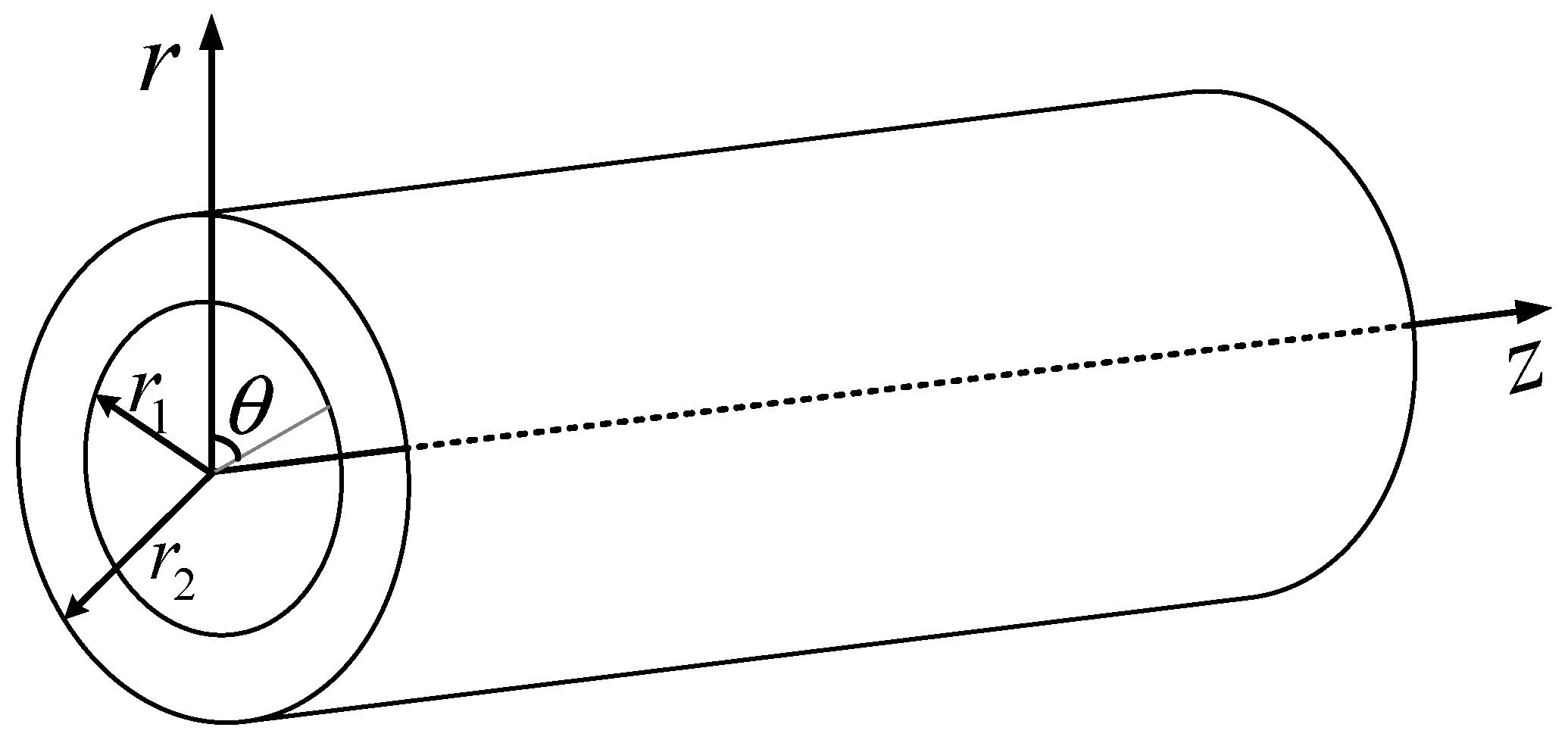
Figure 2.
The matrix and boundary condition distribution of a single-layer fluid-filled elastic tube.
Figure 2.
The matrix and boundary condition distribution of a single-layer fluid-filled elastic tube.
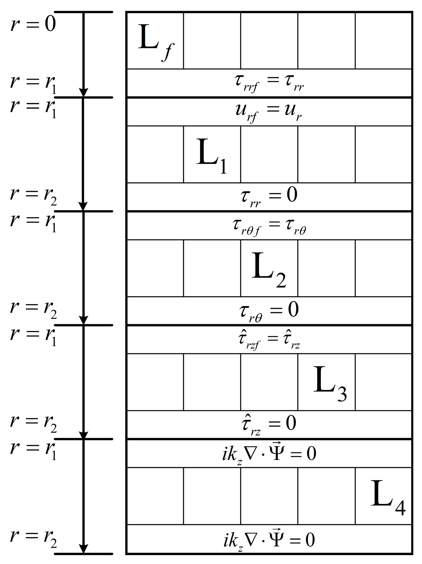
Figure 3.
The flowchart of the proposed spectral method algorithm.

Figure 4.
A two-dimensional model of the water-filled PMMA tube in COMSOL.
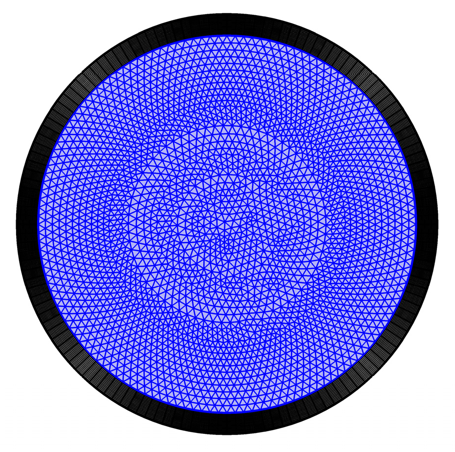
Figure 5.
The difference of between mesh 1–4 and mesh 5 at each mode.
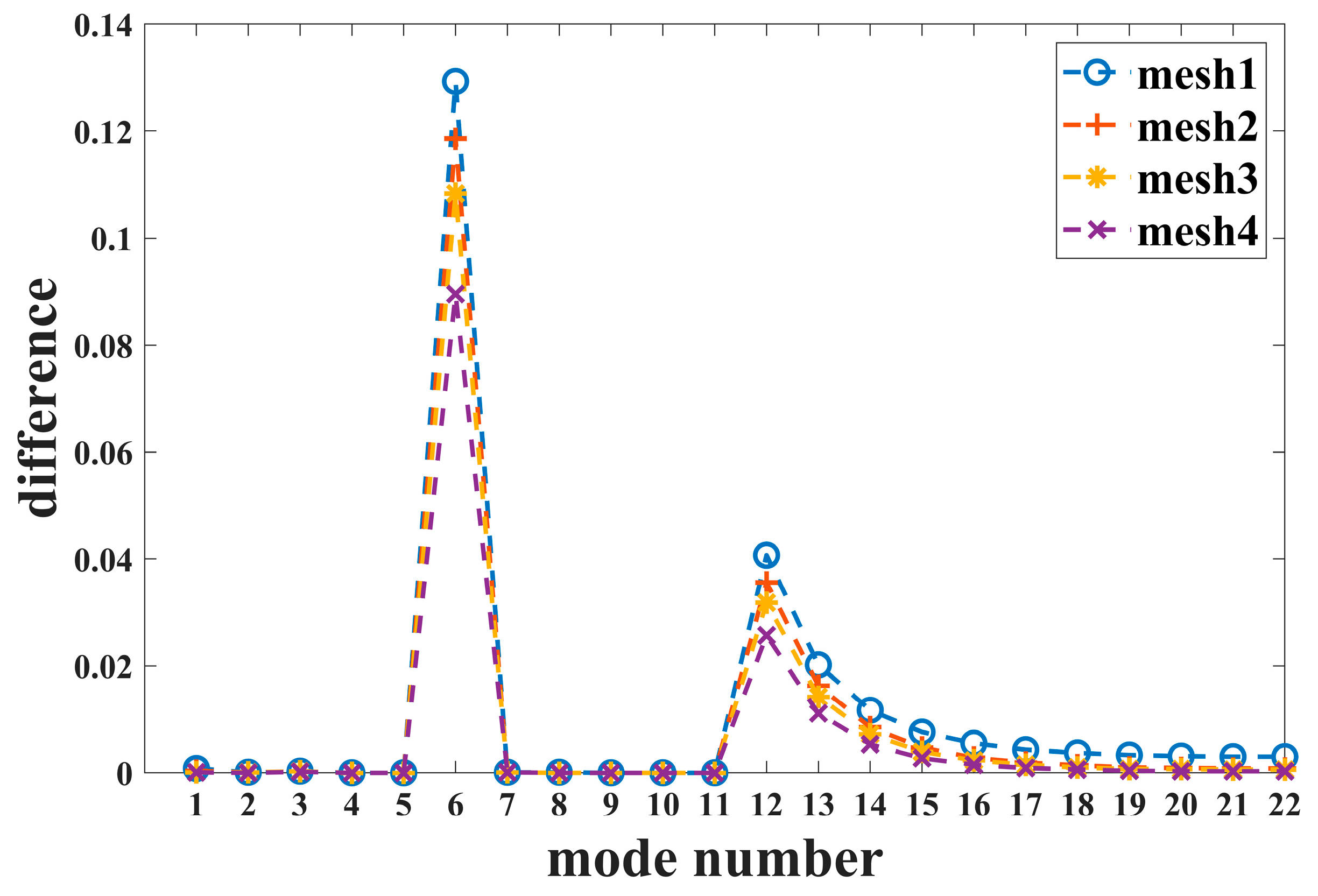
Figure 6.
Comparison of the dispersion curves obtained using the COMSOL simulation and the spectral method algorithm.
Figure 6.
Comparison of the dispersion curves obtained using the COMSOL simulation and the spectral method algorithm.
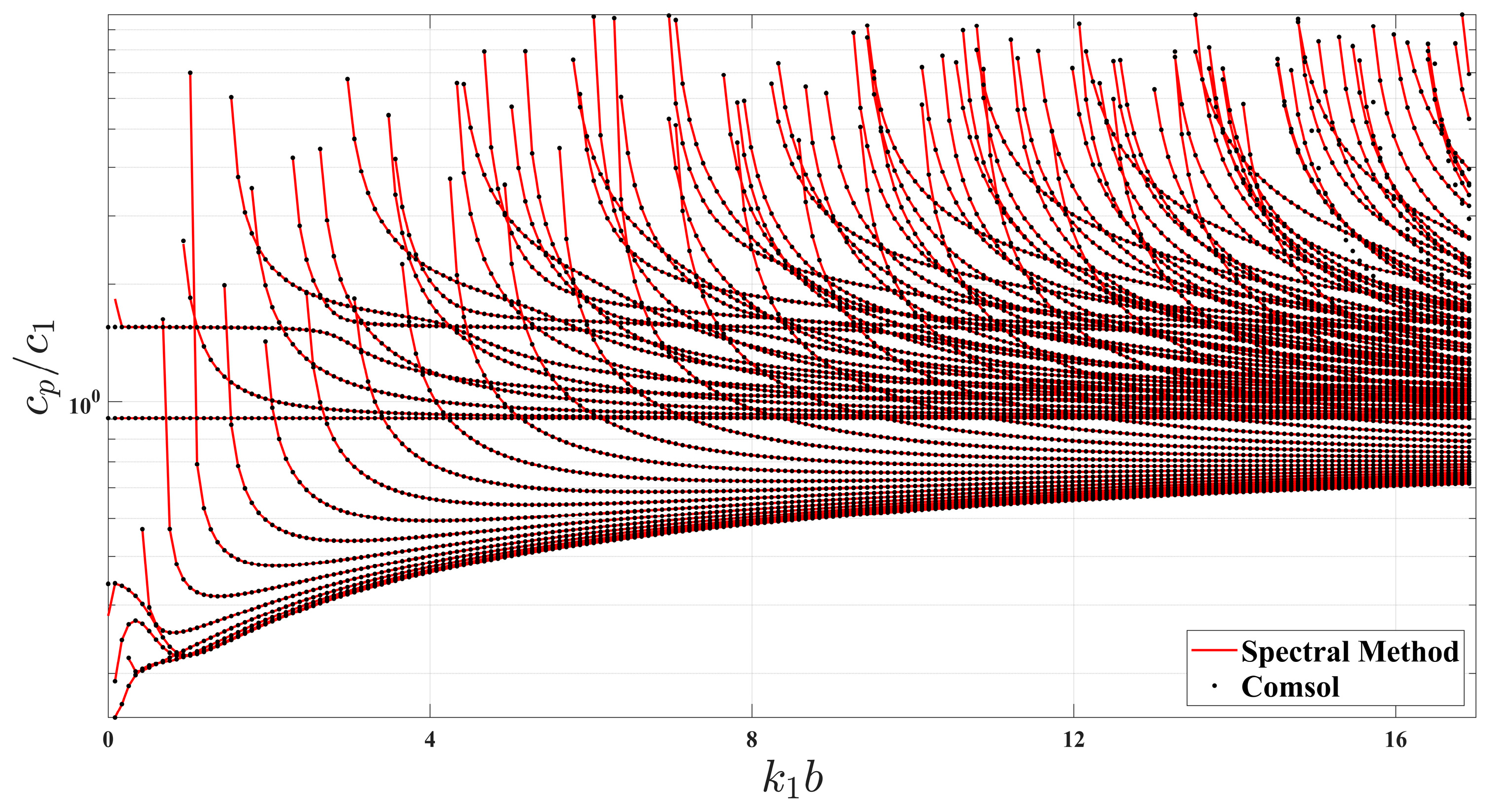
Figure 7.
Comparison of the displacement of the propagation modes in the tube wall between the COMSOL simulation and the spectral method algorithm.
Figure 7.
Comparison of the displacement of the propagation modes in the tube wall between the COMSOL simulation and the spectral method algorithm.

Figure 8.
Phase velocity curves of the water-filled PMMA tube modes: .

Figure 9.
Group velocity curves of the water-filled PMMA tube modes: .

Figure 10.
The radial distribution of the displacement components of the modes at kHz.
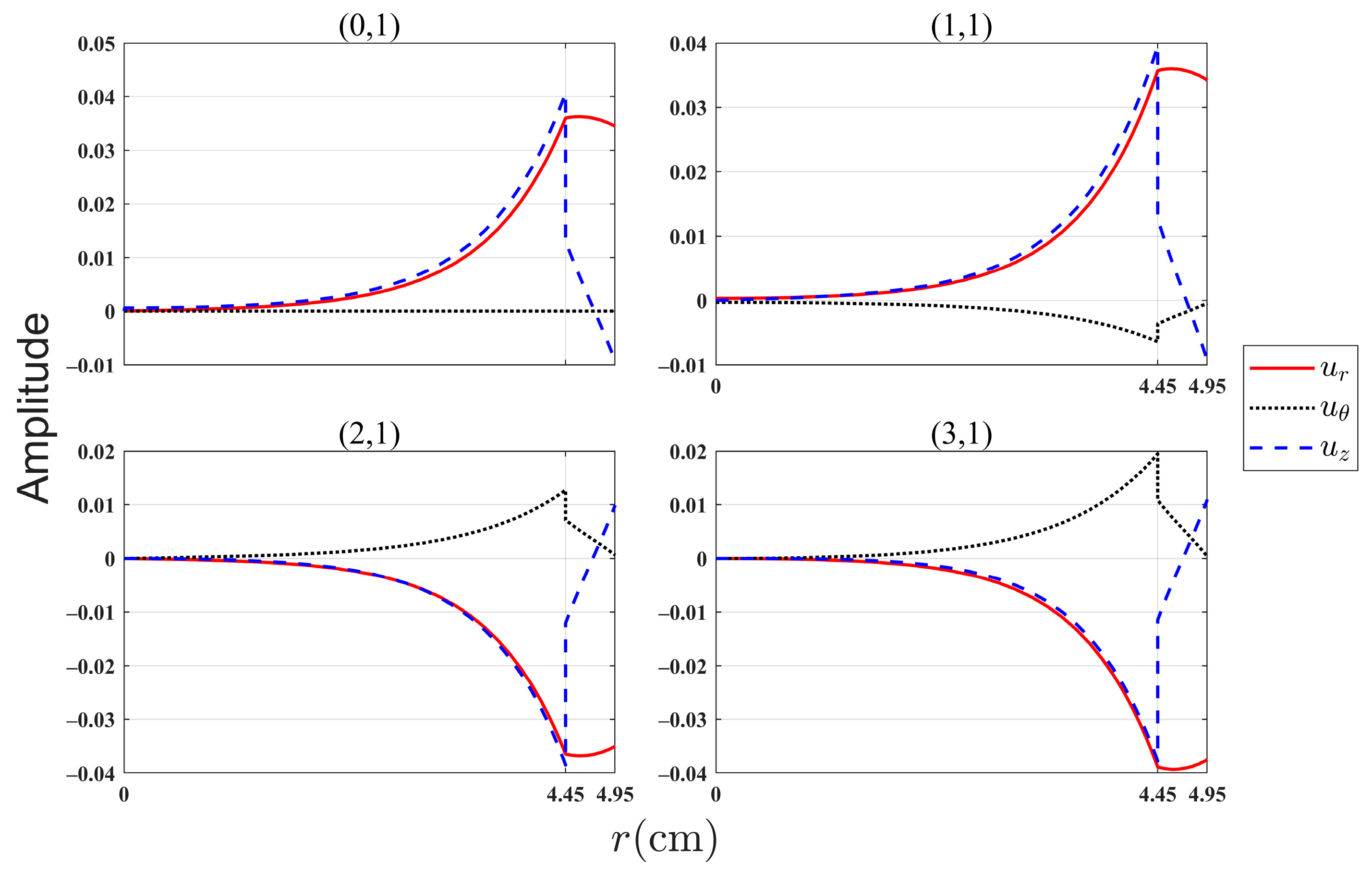
Figure 11.
The radial distribution of the stress tensor components of the modes at kHz.
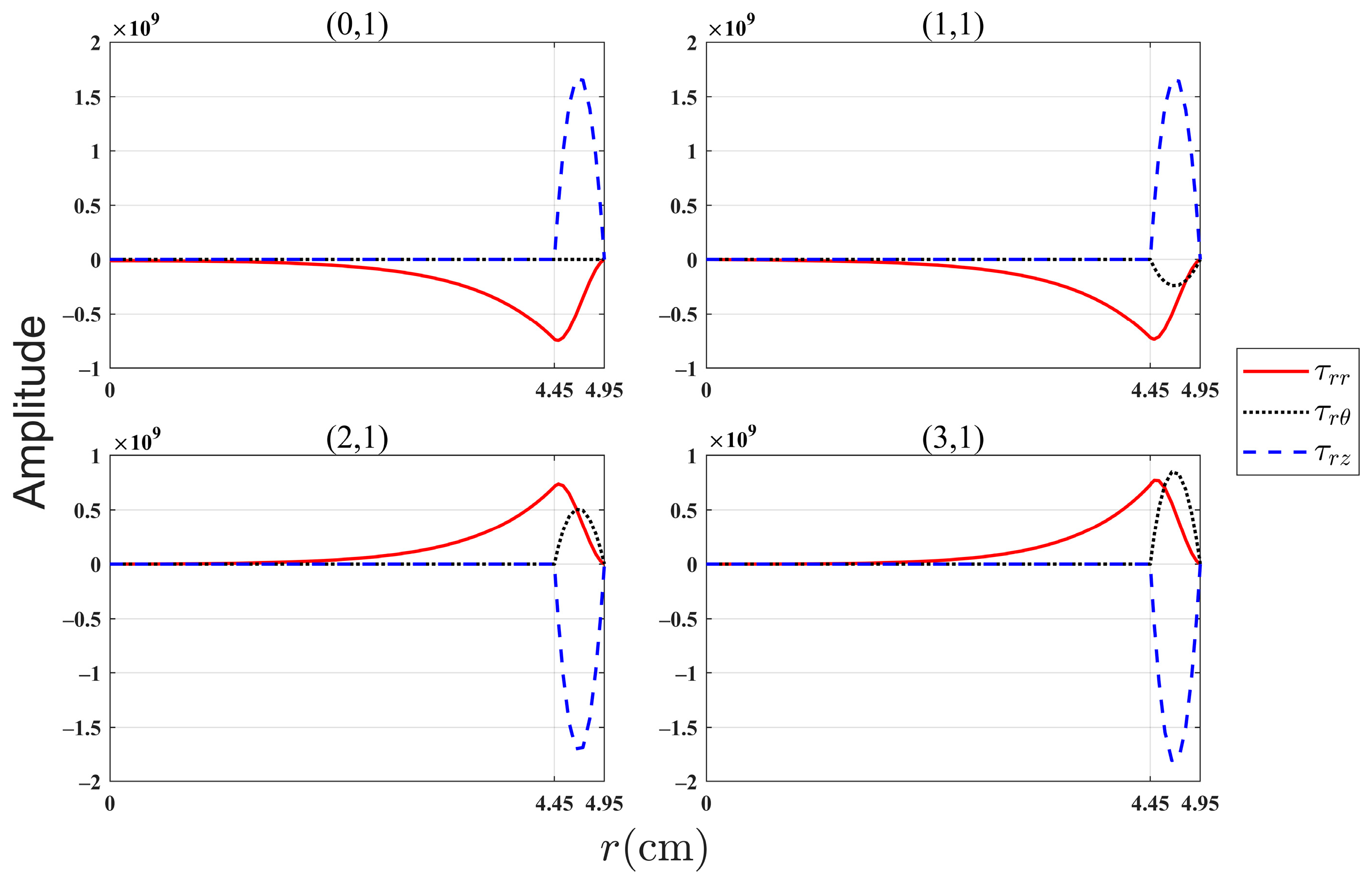
Figure 12.
The cross section of the water-filled multi-layer elastic tube.
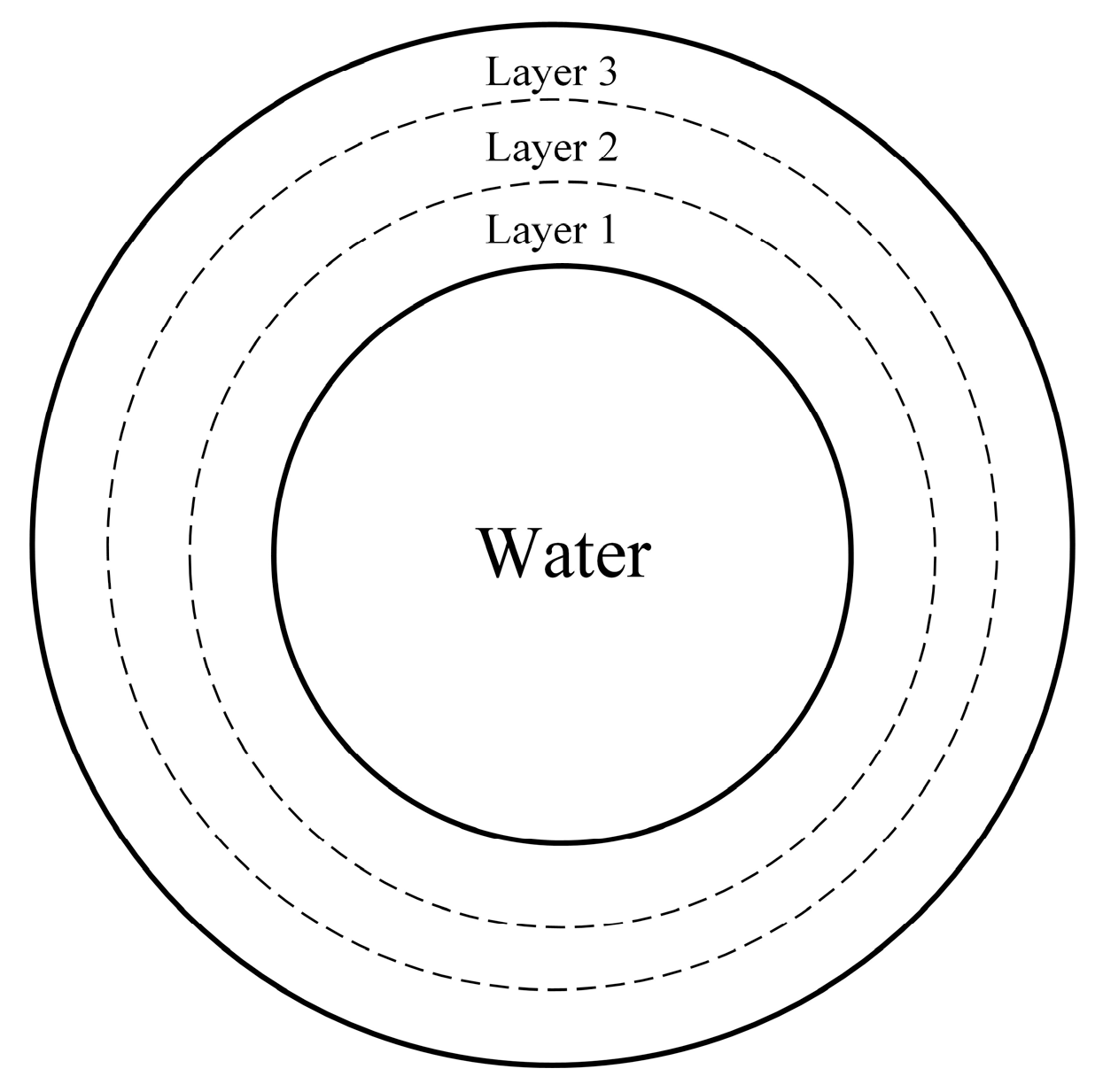
Figure 13.
Phase velocity curves of modes propagating in the water-filled multi-layer elastic tube.

Table 1.
Parameters of the water-filled PMMA tube [26].
Table 1.
Parameters of the water-filled PMMA tube [26].
| (cm) | (cm) | (m/s) | (m/s) | (m/s) | (kg/m3) | (kg/m3) |
|---|---|---|---|---|---|---|
| 4.445 | 0.5 | 2690 | 1340 | 1479 | 1190 | 1000 |
Table 2.
COMSOL mesh file and their numbers of elements.
| Mesh | Mesh 1 | Mesh 2 | Mesh 3 | Mesh 4 | Mesh 5 |
|---|---|---|---|---|---|
| Element Number | 2214 | 3146 | 4644 | 8698 | 27,842 |
Table 3.
The calculation time of the COMSOL simulation and the spectral method algorithm.
| Calculation Methods | Calculation Time |
|---|---|
| COMSOL Multiphysics | Approximately 10 h |
| The spectral method algorithm | A few tens of seconds |
Table 4.
calculated using the COMSOL simulation and the spectral method algorithm at kHz.
| COMSOL Multiphysics | 4.3629 | 21.9621 | 30.1711 | 35.6921 | 37.5116 | 84.0532 |
| 107.1383 | 121.4523 | 130.5509 | 136.0542 | 138.9479 | 139.8424 | |
| Spectral Method | 4.3678 | 21.9621 | 30.1706 | 35.6932 | 37.5116 | 84.0534 |
| 107.1380 | 121.4523 | 130.5509 | 136.0542 | 138.9479 | 139.8424 | |
| Error | 1.12 × 10⁻³ | 0 | 1.66 × 10⁻⁵ | 3.08 × 10⁻⁵ | 0 | 2.38 × 10⁻⁶ |
| 2.80 × 10⁻⁶ | 0 | 0 | 0 | 0 | 0 | |
Table 5.
Modes calculated using the spectral method versus the same modes from Baik [26].
Table 5.
Modes calculated using the spectral method versus the same modes from Baik [26].
| Circumferential Order | Spectral Method Results | Results from Baik [26] |
|---|---|---|
Table 6.
The parameters of the water-filled multi-layer elastic tube.
| Dimension | (cm) | (cm) | (cm) | (cm) |
| 50 | 5 | 5 | 5 | |
| PVC | (m/s) | (m/s) | (kg/m3) | |
| 2388 | 1060 | 1380 | ||
| Iron | (m/s) | (m/s) | (kg/m3) | |
| 5893 | 3230 | 7800 |
Disclaimer/Publisher’s Note: The statements, opinions and data contained in all publications are solely those of the individual author(s) and contributor(s) and not of MDPI and/or the editor(s). MDPI and/or the editor(s) disclaim responsibility for any injury to people or property resulting from any ideas, methods, instructions or products referred to in the content. |
© 2023 by the authors. Licensee MDPI, Basel, Switzerland. This article is an open access article distributed under the terms and conditions of the Creative Commons Attribution (CC BY) license (https://creativecommons.org/licenses/by/4.0/).
Share and Cite
MDPI and ACS Style
Gao, Z.; Li, Q.; Tang, R.; Shang, D. A Spectral Method Algorithm for Modeling the Dispersion of Non-Axisymmetric Modes in Fluid-Filled Elastic Tubes. Appl. Sci. 2023, 13, 12415. https://doi.org/10.3390/app132212415
AMA Style
Gao Z, Li Q, Tang R, Shang D. A Spectral Method Algorithm for Modeling the Dispersion of Non-Axisymmetric Modes in Fluid-Filled Elastic Tubes. Applied Sciences. 2023; 13(22):12415. https://doi.org/10.3390/app132212415
Chicago/Turabian StyleGao, Zirong, Qi Li, Rui Tang, and Dajing Shang. 2023. "A Spectral Method Algorithm for Modeling the Dispersion of Non-Axisymmetric Modes in Fluid-Filled Elastic Tubes" Applied Sciences 13, no. 22: 12415. https://doi.org/10.3390/app132212415
Note that from the first issue of 2016, this journal uses article numbers instead of page numbers. See further details here.