

Vibroacoustic Transfer Characteristics of Underwater Cylindrical Shells Containing Complex Internal Elastic Coupled Systems
1
School of Mechanical Engineering, Shandong University, Jinan 250061, China
2
Key Laboratory of High Efficiency and Clean Mechanical Manufacture, Shandong University, Ministry of Education, Jinan 250061, China
*
Author to whom correspondence should be addressed.
Appl. Sci. 2023, 13(6), 3994; https://doi.org/10.3390/app13063994
Submission received: 16 February 2023
/
Revised: 14 March 2023
/
Accepted: 15 March 2023
/
Published: 21 March 2023
(This article belongs to the Special Issue Advances in Vibroacoustics and Aeroacustics of Marine, Aerospace and Automotive Systems II)
Abstract
:Cylindrical shells containing complex elastic coupling systems are the main structural form of underwater vehicles. Therefore, in this paper, the vibroacoustic radiation problem of underwater cylindrical shells containing complex internal elastic coupling systems is studied. Firstly, the dynamics model of the complex elastic coupled system is established through the method of integrated conductivity. The sound pressure distribution law and the general magnitude relationship between the performance index of hydroacoustic radiation and vibration isolation are investigated through numerical simulation. A strategy of global sensitivity analysis and related parameter optimization is carried out, by applying the Sobol’ method to the dynamics model. It could be concluded that the main flap of sound pressure at low and medium frequencies appears in the direction of the excitation force or the perpendicular to the excitation force, the magnitudes correspondence between the vibration level drop—power flow—hydroacoustic radiation at low frequencies can be expressed as a relatively simple function, and the vibroacoustic transmission of the system at lower order resonance frequencies is dominated by the parameter configuration of the vibration isolation device, while at higher frequencies is more influenced by the modalities of the base structure. The transfer power flow and the level drop are used as objective functions to optimise the acoustic radiation index of the coupled system, with the best results obtained when the transfer power flow and the level drop are used together as objective functions.
1. Introduction
Cylindrical shells are a typical structural form for submarines and other underwater vehicles. A lot of research work has been carried out at home and abroad on the acoustic vibration coupling characteristics of submerged cylindrical hulls, including the case of combined structures with conical hulls and internal reinforcement [1,2,3,4,5,6], but there is still less research work on the acoustic vibration characteristics of hulls containing complex elastic coupling systems. As the power machines inside the underwater vehicle are normally installed in the hull through vibration isolators, the study of dynamics modelling and hydroacoustic radiation characteristics of the underwater cylindrical hull containing complex internal elastic coupling systems would be of theoretical significance and practical value for the optimal design for vibration and noise reduction of underwater vehicles. In vibration isolation systems installed in light elastic structures such as ship shells, the elastic properties of the shell will be significantly reflected in the system responses [7], so the elastic foundation vibration isolation system model is commonly used in theoretical studies, and the common modelling method is to simulate the elastic properties of the installed foundation with beam or plate structures [8,9,10]. However, such theoretical models are still inadequate for underwater vehicle systems. For example, it does not reflect the coupled vibration between the hull and the external hydroacoustic field and the intrinsic connection between the internal vibration isolation design and the external hydroacoustic radiation.
In the analysis of acoustic vibration characteristics of vibration isolation systems, the traditional method is to analyse the influence of various parameters of the coupled vibration system (including the stiffness and mounting position of the isolation support, additional mass, base impedance, etc.) on the force transfer rate, transferred power flow, vibration level drop and other influence laws of the system through the single-factor influence method [11,12,13,14,15,16,17]. This single-factor analysis method belongs to the category of qualitative research, which makes it difficult to evaluate the mutual and combined effects of various characteristic parameters in the system. In addition, there are inevitably errors or uncertainties in the values between the theoretical and actual parameters, and it is not easy to judge the degree of influence on the accuracy of the theoretical analysis results by the single-factor analysis method. Sensitivity analysis is a targeted analysis method for the above problems. In recent years, in the quantitative analysis of structural dynamic characteristics parameters, the more applied is the Sobol’ exponential method global sensitivity analysis. Sobol’ method is a global sensitivity analysis method based on variance proposed by Russian scholar Sobol [18,19,20]. In recent literature reports, most scholars have applied the Sobol’ method for sensitivity analysis and demonstrated the superiority of this method in the optimal design of dynamical systems. Cai Qiang [21] designed a new magnetorheological suspension, performed a global sensitivity analysis and explored the optimal design method of magnetorheological suspension. Yang Qinghua [22], who proposed a magnetorheological suspension scheme with a mixed mode of flow and squeeze with the objective of improving the NVH performance in the vehicle, conducted a sensitivity analysis of the model and proposed a multi-objective optimization method for its parameters. Du Huanyu and Li Hongguang [23] used a super-large shaker as the research object and carried out a sensitivity analysis and optimization of each main structural parameter to improve the axial resonance frequency of the structure. Li Rui [24] applied the Sobol’ sensitivity analysis method and the local method to investigate the role of nonlinear terms and other structural parameters on the resonant angular frequency and transmission rate in a nonlinear passive vibration isolator. In contrast, the application of sensitivity analysis to the analysis of acoustic vibration characteristics of elastic foundation vibration isolation systems within submerged shell structures has not yet been reported.
In this paper, combine the Helmholtz equation, the plate and shell vibration equation and the sub-structure conduction synthesis method to establish a dynamical model of the coupled system of vibration source machine—floating raft device—thin cylindrical shell—hydroacoustic field. As a result, analytical solutions were obtained for the vibration power flow, vibration level dropout, hydroacoustic radiation power and sound pressure at the field point of the coupled system; furthermore, the sound pressure distribution of the radiated hydroacoustic field, the general magnitude relationship between the vibration isolation performance evaluation index and the hydroacoustic radiation characteristics index were analysed. Based on the above work, the global sensitivity analysis of Sobol’s exponential method to quantitatively study the influence of the system characteristics parameters on the transfer power flow and vibration level dropout and the degree of interaction in the frequency domain were applied; then the optimal design of the coupling system was carried out.
The paper is organized as follows. Section 2 develops a dynamical model of a submerged cylindrical shell containing a complex elastic coupled system and solves the analytical solutions and Section 3 analyses the sound pressure distribution law of the coupled system and then studies the numerical correspondence between the vibration isolation performance index and the sound radiation characteristics index. A global sensitivity analysis of the coupled system and optimization of the structural parameters are analysed in Section 4. Finally, Section 5 draws the conclusions from the study conducted.
2. Theoretical Models
2.1. Conductivity Analysis of Coupled System Substructures
In view of the increasing use of floating raft vibration isolators in various ship systems, this paper presents a dynamic modelling and dynamic response solution for the coupled system of the vibration source machine—floating raft device—thin cylindrical shell—hydroacoustic field in Figure 1, then carries out a numerical simulation of the acoustic vibration characteristics of the coupled system.
In Figure 1, vibration source machines A1 and A2 (simulating multiple units) are installed on the floating raft R. Each machine is installed on the raft by four elastic supports, and the raft is connected with the thin cylindrical shell by four elastic supports. The rectangular coordinate system Oxyz is established, where Oz axis is the center line of the cylinder, and the Oy axis is the vertical line. In order to simplify the analysis, only the vertical translational vibration and rotational vibration around Oz or Ox axis of the system is considered. Therefore, the vertical exciting force F1, F2 and excitation torque T1, T2 in the direction of Oz axis to the center of mass of each machine is applied. In addition, set machine A1, A2 and R are symmetrical about the yOz plane, and the figures of b1, b2, h1z, h2z, h1x, h2x, Hz, Hx and LR is the relevant installation dimensional parameter of the system, while σ1, σ2, σ3, σ4 indicates the connection point between the vibration isolation support below the floating raft and the thin cylindrical shell.
Figure 2 decomposes the system in Figure 1 into three subsystems according to the power transfer relationship: the source machine (A), the floating raft device (B) and the submerged cylindrical shell (C), where the submerged cylindrical shell contains the acoustic coupling between the thin cylindrical shell and the peripheral hydroacoustic field. In Figure 2, Fe = [F1, T1, F2, T2]T is the excitation vector acting on the source device, FA, FB1, FB2 and FC are the dynamic forces transmitted by the floating raft device at its coupling points with the source device and the shell (vectors) and VA1, VA2, VB1, VB2 and VC are the velocity responses at the corresponding coupling points (vectors).
The dynamic transfer characteristics of the vibration source machine A, the floating raft device B and the submerged cylindrical shell C are described in terms of the conductance matrices A, B and C, respectively.
From the relationships described above, it is possible to derive
According to the structure of the system in Figure 1, set m1, J1x, J1z and m2, J2x, J2z to be the masses of machines A1 and A2, respectively, and the rotational inertia around their centres of mass and parallel to the axes Ox and Oz. The derivative matrix of the vibration source machine A is:
where, for i = 1 or 2, , , , ; Xi and Zi are the coordinate vectors of the machine mounting support positions, , ; Ode notes a matrix whose elements are all 0, Il × n is an l × nl × n dimensional matrix whose elements are all 1.
For the floating raft unit B, let the four vibration isolators under units A1, A2 and raft frame R all have the same complex stiffness, which are denoted as k1, k2 and kR respectively. Neglect the mass of the vibration isolators and denote mR as the mass of the raft frame, and set JRx and JRz as the rotational inertia of the raft frame around its centre of mass parallel to Ox and Oz respectively, then
where XR1, XR2, ZR1, ZR2 are the coordinate vector of the vibration isolation support connected to the floating raft, XR1 = [0.5h1x, 0.5h1x, −0.5h1x, −0.5h1x, 0.5h2x, 0.5h2x, −0.5h2x, −0.5h2x], XR2 = [0.5Hx, 0.5Hx, −0.5Hx, −0.5Hx], ZR1 = [−b1 − 0.5h1z, −b1 + 0.5h1z, −b1 − 0.5h1z, −b1 + 0.5h1z, b2 − 0.5h2z, b2 + 0.5h2z, b2 − 0.5h2z, b2 + 0.5h2z], ZR2 = [−0.5Hz, 0.5Hz, −0.5Hz, 0.5Hz]; El × n is an l × n dimensional matrix.
For the thin submerged cylindrical shell C, its conductance matrix is a square matrix of order 4 × 4 under the structure of the system in Figure 1
where . This is defined as the velocity response in the direction of the support force at the joint between the vibration isolator and the thin cylindrical shell, when a unit excitation is applied in the direction of the support force at the joint between the vibration isolator and the thin cylindrical shell.
Since the coupling between the vibration of the thin cylindrical shell underwater and its external hydroacoustic field cannot be ignored, the vibration of the thin cylindrical shell with the Helmholtz equation is combined to solve the derivative function of the thin cylindrical shell underwater analytically.
2.2. Solving for the Conductance Function of a Thin Underwater Cylindrical Shell
Establish the (r, φ, z) cylindrical coordinate system on the middle surface of the thin cylindrical shell, and let the origin of the coordinates lie at the centre of the circle on the left face of the cylindrical shell, r and z are the distances from the spatial point σ(r, φ, z) to the central axis and the left face of the thin cylindrical shell respectively, and φ is the angle at which σ(r, φ, z) deviates from the vertical direction; the transformation relationship between cylindrical coordinates and Cartesian coordinates is: x = rcosφ, y = rsinφ, z = z.
Set the length of the thin cylindrical shell as L, the thickness as d and the radius of the middle surface as a (d/a ≤ 0.05); the density, Poisson’s ratio and modulus of elasticity of the cylindrical shell material are set as ρ,μ,E, respectively. Apply a simple harmonic excitation force Fz·ejω along the axial direction (z coordinate axis direction) at the inner side of the thin cylindrical shell σe(φe, ze).Let u(z, φ, t) = U(z, φ)·ejωt, v(z, φ, t) = V(z, φ)·ejωt, w(z, φ, t) = W(z, φ)·ejωt denote the vibrational displacement of the point σ(φ, z) on the cylindrical shell in the z,φ,and r coordinate directions, respectively, then u,v and w satisfy the following differential equations of motion [25].
where p is the radiated hydroacoustic pressure generated on the outside of the thin cylindrical shell due to its vibration; S1, S2, S3 are differential operators, and
where , .
The sound pressure (p = P(r, φ, z)·ejωt) of the water sound field outside the thin cylindrical shell satisfies the Helmholtz equation [26].
where k is the number of waves, k = ω/c0, c0 is the wave speed (c0 ≈ 1500 m/s in water).
On the dividing surface between the thin cylindrical shell and the external hydroacoustic field, there are the following boundary conditions:
where ρ0 is the sound field medium density.
The vibration displacements U, V and W of a thin cylindrical shell can be expressed as a superposition of vibration patterns
where qij is the modal influence factor; Uij, Vij, Wij are the vibration functions, Aijαj(z), Bijβj(z) and Cijγ j(z) are determined by the boundary conditions of the cylindrical thin shell. Apply the variational separation method and the Fourier integral method to the Helmholtz equation (Equation (9)) and note that P(r, φ, z) is periodic with respect to φ; it can be shown that P has the following form of a series solution:
where Hi(2)(krr) is the second class i-order Hankel function, and kr2 = k2 − τ2.
Substituting the above equation and Equation (3) of Equation (11) into the boundary conditions (Equation (10)) and apply a Fourier transformation to the variable z on both sides of the equation. By comparing the coefficients it is possible to obtain a solution for the sound pressure level expressed in terms of the modal influence factor qij and the vibration shape function Cijγ j(z)
where .
To obtain the final modal impact factor qij, let r = a in Equation (13) and substitute it into Equation (8), and then use the orthogonality of the vibration function to obtain a linear system of equations for the modal impact factor qij
where Mij and ωij are the modal masses and modal frequencies of the cylindrical thin shell corresponding to the modes Uij, Vij and Wij, respectively.
Organizing Equation (14) into matrix form, that is, GQ = Fz, Q is a column vector consisting of the modal influence factor qij, G is a list square of the corresponding coefficients of qij, and Fz is a modal force vector consisting of FzAijαj(ze) on the right-hand side of each equation of Equation (14), then Q = G−1Fz.
After the modal influence factor is obtained, substitute into Equations (11) and (13) respectively to obtain the vibration displacement responses U(z, φ),V(z, φ),W(z, φ) and the external hydroacoustic field sound pressure P(r, φ, z) of the cylindrical thin shell, and also the displacement derivative function of the axially concentrated excitation force Fz·ejωt for the three coordinate directions (i.e., axial, tangential and radial) of z,φ and r: Yuu(σ, σe) = U/Fz, Yvu(σ, σe) = V/Fz, Ywu(σ, σe) = W/Fz.
Similarly, a simple harmonic excitation force Fφ·ejωt along the tangential direction (in the direction of the φ coordinate axis) or a simple harmonic excitation force Fr·ejωt along the radial direction (in the direction of the r coordinate axis) can be applied to the inside of the thin cylindrical shell σe(φe, ze), the displacement derivative functions of the tangential or radial concentrated excitation on the three directions z,φ and r are obtained according to the same method as above and are noted as Yuv(σ, σe), Yvv(σ, σe), Ywv(σ, σe), Yuw(σ, σe), Yvw(σ, σe), Yww(σ, σe). For the case of applied tangential excitation, it is noted that the symmetric nature of the cylindrical thin shell and sound field modes is different from the case of axial and radial excitation, and Equations (11) and (13) need to be modified as
Directional conductance along any direction can be calculated using the nine conductivity functions described above. Let σi(a, φi, zi) be the coordinates of the cylindrical coordinate system (i = 1, 2, 3, 4) in the coupling point between each vibration isolation support and the thin cylindrical shell in the system of Figure 1, then the point and transfer conductance cij in Equation (7), according to its definition, can be calculated by the following equation:
Figure 3 shows an example of the calculation results for the vertical conductance of the thin cylindrical shell of Figure 1. Due to the complexity of the calculations, Figure 4 compares the results of the hydroacoustic pressure calculations obtained by the above analytical algorithm with the results of the finite element method obtained from the LMS Virtual Lab software environment for the same structural parameters, in order to check the reliability of the analytical model. It is clear from the comparison that the results of the two methods are in general agreement. The individual peaks in the graph are resonance peaks, which are the result of the resonance of the coupled system at this excitation force. However, the resonant peak frequency of the thin cylindrical shell obtained from the vitural.lab simulation is slightly lower than the resonant peak frequency of the analytical solution. This is due to the fact that vitural.lab uses an AML layer approach for the infinite waters wrapped around the outside of the thin cylindrical shell, which ignores a large amount of water mass and thus leads to the advancement of the resonant peak of the thin cylindrical shell.
2.3. Level Drop, Transmitted Power Flow, Sound Pressure at the Hydroacoustic Field and Total Radiated Sound Power of the Coupled System
For elastic foundation vibration isolation systems, the transferred power flow (the time-averaged power of the excitation forces transmitted to the foundation structure through the isolation bearings) is a theoretical indicator for evaluating the effectiveness of vibration isolation design. However, as the transferred power flow is difficult to measure in practice, the effect of the actual vibration isolation system is generally assessed by measuring the vibration level drop. For the system in Figure 1, the transmitted power flow and vibration level drop can be combined with the sound pressure and radiated sound power of the water acoustic field to make a comprehensive analysis and evaluation of the acoustic vibration characteristics of the coupled system.
After substituting the results of Equation (17) into Equation (7), the excitation force FC transmitted to the cylindrical shell through the vibration isolation support can be obtained from Equation (3), and then the velocity response VC of the cylindrical shell at the point of coupling with the vibration isolation support can be derived from Equation (2) of Equation (3), so the transferred power flow of the system can be known as
where the superscript “H” indicates the Hermitian transpose.
The vibration level drop of the floating raft isolator is the ratio of the mean square value of the acceleration response (in dB) between the isolator and the base structure (here the base structure is a thin cylindrical shell) and the junction point of the vibration source equipment, so it is
where VA2 is calculated from Equation (4).
In order to calculate the radiated hydroacoustic field formed by the excitation of FC = [FC1, FC2, FC3, FC4]T in the cylindrical thin shell in the coupled system of Figure 1, take out the elements FCi (i =1, 2, 3, 4) in FC in turn. Decompose these elements orthogonally along the axial, tangential and radial directions of the thin cylindrical shell as Fzi, Fφi, Fri, then note the sound pressure generated by the action of Fzi, Fφi, Fri as Pzi(r, φ, z), Pφi(r, φ, z), Pri(r, φ, z); they can all be calculated from Equation (8) to Equation (16), while the total sound pressure P at any field point σ(r, φ, z) in the hydroacoustic field is the superposition of each of the above Pzi, Pφi, Pri:
The above principle of solving for sound pressure is also fully applicable to the solution of the vibration response of the cylindrical thin shell. Let the radial displacement response of the thin cylindrical shell under the action of Fzi, Fφi and Fri be Wzi(φ, z), Wφi(φ, z), Wri(φ, z), as obtained from Equation (8) to Equation (16). Then the displacement response W(φ, z) of the thin cylindrical shell under the joint action of all FCi (i = 1, 2, 3, 4) is obtained by superimposing each Wzi, Wφi, Wri.
After obtaining the sound pressure P and the radial displacement response W of the cylindrical thin shell, the total radiated sound power of the cylindrical thin shell is
where the superscript “*” indicates that the complex conjugate is taken.
3. Analysis of Acoustic Vibration Transfer Characteristics of Coupled Systems
3.1. Structural Parameters of the Coupling System
Next, through numerical simulations of the acoustic vibration transfer characteristics of the system in Figure 1, carry out a theoretical analysis of the sound pressure distribution pattern of the peripheral hydroacoustic field of the thin submerged cylindrical shell containing the internal complex coupled system, and the numerical correspondence between the sound pressure at the field points and the transferred power flow, the vibration level drop and the acoustic radiated power of the system.
According to the general guidelines for vibration isolation design, Table 1 shows the basic parameter settings for the floating raft system. To avoid the chance of numerical analysis, three sets of parameter configurations are given here.
Let the material of the thin cylindrical shell be steel (modulus of elasticity E = 2.1 × 10¹¹ Pa, Poisson’s ratio μ = 0.28, density ρ = 7800 kg/m3, damping loss factor ξ = 0.01), radius a = 0.2 m at the centre, length L = 1 m, thickness h = 0.005 m. The fluid outside the cylindrical shell has density ρ0 = 1000 kg/m3 and sound velocity c0 = 1500 m/s. The excitation amplitude F1 = F2 = 1N.
To simplify the calculation without loss of generality, the boundary conditions of the cylindrical shell are chosen to be simply supported at both ends. The simply supported boundary condition of a cylindrical thin shell is that which constrains its external normal direction and circumferential displacement at the z = 0 and z = L boundaries to 0, while leaving the axial displacement and the external normal deflection at the end face unconstrained.
According to the Navier solution, for the vibration functions Aijαj(z), Bijβj(z), Cijγ j(z) in Equations (11) and (15), it is advisable to take αj(z) = cos(jπz/L), βj(z) = γj(z) = sin(jπz/L), [Aij, Bij, Cij]T is the eigenvector of the square matrix A of Equation (24); the intrinsic frequency of the thin cylindrical shell ωij2 = λij2E/[ρ(1 − μ)], λij2 is the eigenvalue of square matrix A corresponding to [Aij, Bij, Cij]T; the modal masses Mij of each order of the cylindrical thin shell is: M00 = 2πaLρd (i = j = 0), Mi0 = πaLρd (i ≠ 0, j = 0), M0j = πaLρd[A0j2 + B0j 2 + C0j2] (i = 0, j ≠ 0), Mij = 0.5πaLρd(Aij2 + Bij 2 + Cij 2) (i ≠ 0, j ≠ 0).
3.2. Patterns of Sound Pressure Distribution
Figure 5 shows the sound pressure directivity diagram for different frequencies, different axial distances and different radial distances,
In Figure 5, the coordinates of the sound pressure observation point are defined in cylindrical coordinates (rp, p, zp). rp represents the radial distance from the observation point to the axis of the thin cylindrical shell, zp represents the axial distance from the observation point to the left end face of the thin cylindrical shell and p represents the angle of deviation of the observation point from the vertical direction.
3.3. Analysis of the Numerical Correspondence between Vibration Isolation Performance Indicators and Sound Radiation Characteristics Indicators
It is generally accepted that the vibration level drop or the transmitted power flow can be used as a useful indicator to evaluate the effectiveness of vibration isolation, the former showing the degree of attenuation of the vibration level after passing through the isolation device, and the latter showing the level of vibration energy entering the receptor. Figure 6 compares the spectrum of the vibration level dropout and the spectrum of the transmitted power flow for the three different operating conditions in Table 1. They have different magnitudes, but show a similar decay trend with increasing frequency; at the same time, excluding the individual peaks near the fundamental frequency, most of the peak frequencies of the two have a one-to-one correspondence.
Figure 7 plots the spectrum of the transmitted power flow, the spectrum of the water acoustic pressure amplitude and the spectrum of the cylindrical shell acoustic radiation power together for comparison; 1, 2 and 3 in the figure represent the transmitted power flow, the water acoustic pressure amplitude and the cylindrical shell acoustic radiation power respectively. Noting that the water sound pressure varies with the field point, so chose (1270°,1) as the sound pressure observation point here according to the water sound pressure distribution pattern in Figure 5. Firstly, the spectral shape of the sound pressure amplitude and the sound radiated power is basically the same, including its peak frequency and the variation pattern with frequency. Secondly, the transmitted power flow also has a relatively perfect correspondence with the peak frequency of the acoustic radiated power. There are also some obvious differences between them. In the low frequency band, the acoustic radiated power is significantly smaller than the transmitted power flow, due to the structural damping of the thin cylindrical shell consuming more vibration energy at low frequencies; as the frequency increases, the spectra of the transmitted power flow and the acoustic radiated power gradually tend to coincide, but there are still obvious differences between the two near the resonant frequency of the system.
In order to compare the magnitudes of these indicators more clearly, the ratios 1, 2 and 3 in Figure 8 show the ratio of transmitted power flow to sound pressure amplitude, transmitted power flow to sound radiated power and sound pressure amplitude to sound radiated power for (ratio of decibel values). As can be seen from Figure 8, a linear proportionality between sound pressure and radiated power is evident (ratio 3); and it also seems to be a relatively stable proportionality between transmitted power flow and sound pressure (radiated power). Especially the ratio of radiated power to transmitted power flow (ratio 2) increases approximately linearly in lower frequency and converges to 1 in higher frequency; the ratio of sound pressure amplitude to transmitted power flow (ratio 1) is more stable in the lower frequency bands. The ratio of sound pressure amplitude to transmitted power flow (ratio 1) is similar to ratio 2 in overall trend, but the former has a larger peak fluctuation. However, the former has greater peak fluctuations in the higher frequency domain, indicating a greater uncertainty in the numerical correspondence between the transmitted power flow and the far-field sound pressure.
Given the difficulty of actually measuring the transmitted power flow, the idea of predicting the acoustic radiation performance of the receptor in terms of the level drop of a vibration isolation system is relatively attractive. Therefore, Figure 9 shows the ratio of the transmitted power flow to the level drop (difference in decibel values). It can be observed through Figure 9 that the ratio curve of the transmitted power flow to the level dropout has a relatively regular linear or approximately linear nature, but this linear relationship is broken by the peak of the curve around the intrinsic frequency of the system. In the mode-sparse low frequency domain, it is relatively easy to obtain this linear relationship; however, in the mode-dense high frequency domain, near the intrinsic frequency of the coupled system, it will be more difficult to obtain a numerical correspondence between them. Furthermore, it is noted that the magnitudes of the vibration level dropout and the transferred power flow are different, so that their ratio curves fluctuate as a whole with the magnitude of the excitation.
Based on the above analysis, the numerical correspondence between the vibration level dropout—power flow—hydroacoustic radiation can be expressed as a relatively simple function in the low frequency phase, which can provide guidance for the design and test diagnosis of practical vibration and noise reduction. However, if the relationship is extended to the high frequency domain, there is a large uncertainty due to the influence of the coupled system vibration modes. In the following section, a further theoretical discussion of the optimisation of structural parameters based on level dropout, transferred power flow and acoustic radiation objective functions is presented in conjunction with the Sobol’ sensitivity analysis method.
4. Global Sensitivity Analysis and Optimisation for Structural Parameters of Coupled Systems
4.1. Sensitivity Theory
Complex dynamical systems have many influencing parameters and the acoustic characteristics of the coupled system vary for different values and combinations of various parameters. The influence of various structural parameters on the isolation effect in vibration isolation systems has been studied extensively in the past, but mainly by means of the single factor method. Sensitivity analysis focuses on identifying the importance of the influence of different structural parameters on the target function and can show the degree of interaction between different structural parameters.
The core idea of Sobol’ sensitivity analysis is to decompose the function Y into a sum of subterms in the case where the input parameter domain Ik is a k dimensional unit cell
where is the ith parameter, is a constant, and the remaining subterms have zero integration over any variable they contain
Sub-terms are orthogonal to each other, so if (i1, i2, …, is) ≠ (j1, j2, …, jl), then
Due to the above relationship, the decomposition of Equation (25) is unique and the subterms can be found by multiple integration
Assuming that f(X) squared is productable, square both sides of Equation (25) and integrate over the entire domain of definition yields
From this, define the total variance of f(X)
and the bias variance of
The global sensitivity can therefore be expressed as
Si is the first-order sensitivity coefficient of the factor xi and represents the main effect of xi on the output (the effect of xi on f(X)); Si,j (i ≠ j) is the second-order sensitivity coefficient and represents the cross-effect of the two parameters xi, xj (the sum of the effects of xi, xj alone cannot directly represent the changes caused by them), and
Therefore, the total sensitivity coefficient is the sum of the order sensitivity coefficients of a variable, which can be expressed as
In Equation (34), is the sum of the variances of the other input variables excluding the variable xi.
4.2. Global Sensitivity Analysis of Coupled Systems
Based on the viewpoint of vibration and noise reduction design, take the transmitted power flow, vibration level dropout and acoustic radiated power as the objective functions, respectively, then apply Sobol’ sensitivity analysis to compare and analyse the influence weights and cross-influence weights of various structural parameters of the coupled system in Figure 1 on the above three objective functions. This analysis provides a theoretical reference for the optimisation of the vibroacoustic transfer characteristics of similar systems.
In order to introduce the Sobol’ sensitivity analysis method, first define the interval of variation and the probability distribution of each parameter. Without loss of generality, the distributions of all parameters are set to follow a normal distribution. Since the magnitudes of the different parameters differ, the standard deviation is designed according to the coefficient of variation , where m is the mean and s is the standard deviation. Let cu = 0.01 and use ladin hypercube sampling; Table 2 lists the means, variances and ranges of variation of various parameters. To ensure the accuracy of the calculation and to take into account the length of the calculation, set the sample size of sampling N = 2000.
Figure 10 compares the coupled system at the first 5 orders of resonant frequency. The first-order and total sensitivities of the various parameters are listed in Table 2 for the transmitted power flow, vibration level dropout and acoustic radiated power; where a larger first-order sensitivity represents a greater effect of the parameter on the target function, and a larger difference between the first-order sensitivity and the total sensitivity represents a greater effect of the interaction of the parameter with the other parameters on the target function. The resonant frequency points were chosen for sensitivity analysis because they correspond to the peak points of the target function, so that the magnitude of the change in the target function is larger and therefore also has a higher sensitivity value.
According to Figure 10, at the lowest order resonant frequencies (Figure 10a–f, f = 15 Hz, 38 Hz), the vibroacoustic transmission o1f the system is more influenced by the parameter configuration of the vibration isolators, as their vibration modes are mainly determined by the vibration isolation system inside the thin cylindrical shell; at higher frequencies (Figure 10g–o, f = 132 Hz, 194 Hz, 264 Hz), the influence of the parameter configuration of the vibration isolators tends to diminish and the influence of the modalities of the receptor structure dominates. The weighting of the influencing parameters at different frequencies is different, but in all cases the thickness d of the thin cylindrical shell is a highly sensitive influencing parameter, indicating that the influence of the structural properties of the receptor on the vibroacoustic transmission cannot be ignored. The sensitivity analysis also allows for the elimination of factors that have a small influence on the vibroacoustic transmission, such as the spacing parameters h1x, h2x, h1z, h2z of the upper vibration isolator. It is also noted that although the transmitted power flow, the vibration level dropout and the acoustic radiation power have some intrinsic mechanistic link and numerical correspondence, a sensitivity analysis with each of them as an objective function will result in different parameter influence. This is related to the local mathematical nature of the function at a particular frequency. It is worth pointing out that this example seems to indicate a high degree of similarity between the sensitivity calculations for the level drop and the acoustic radiated power, which means the parameters that have a greater influence on both at different frequencies are essentially the same.
Collect the parameters with a large influence weight on all frequencies, and then the object of structural parameter optimisation for the specified objective function is specified.
4.3. Optimisation of Structural Parameters of Coupled Systems Based on Sensitivity Analysis
For submarines and other underwater vehicles, the reduction of acoustic radiated power is the ultimate goal of dynamic structural optimization design, but the actual system’s acoustic radiated power function is difficult to obtain, so other relatively easy to obtain vibroacoustic transfer characteristic functions are considered instead of acoustic radiated power as the structural optimization objective function.
The basic correspondence between level drop—transmitted power flow—acoustic radiated power has been described through the previous analysis, so in the following, select the transmitted power flow (method 1), level drop (method 2) and transmitted power flow + level drop (method 3) as the objective functions based on the model in Figure 1 (as shown in Table 3), and further discuss the optimal design method for vibration and noise reduction of the coupled system.
In Table 3, , are the root mean square of the power flow and the vibration level drop, respectively. According to the sensitivity analysis in the previous section, set the parameters that have a greater influence on the transmitted power flow (Method 1) and the vibration level drop (Method 2) as the optimisation variables, including the lower vibration isolator spacing Hx, the upper unit 1 mass m1, the raft frame mass mraft, the upper vibration isolator stiffness k2, the lower vibration isolator stiffness kR, the circular thin shell thickness d and the vibration isolator loss factor η. Table 4 shows the range of values for each parameter variable set for further optimisation calculations. In order to ensure structural stability while obtaining a more pronounced optimisation effect, the range of variation of the parameters is set to μ ± 30σ, using the Latin hypercube sampling method. The values of the parameters that are not set as optimisation variables in the optimisation calculation are still shown in Table 2.
Adopt the NSGA-2 algorithm for the coupled system model, set the NSGA-2 operation parameters as the population number 100, the iteration number 100, and the crossover frequency 0.7. After the iterative calculation is completed, the results are kept in three valid digits, and the optimized structural parameters of the coupled system are obtained as shown in Table 5 below.
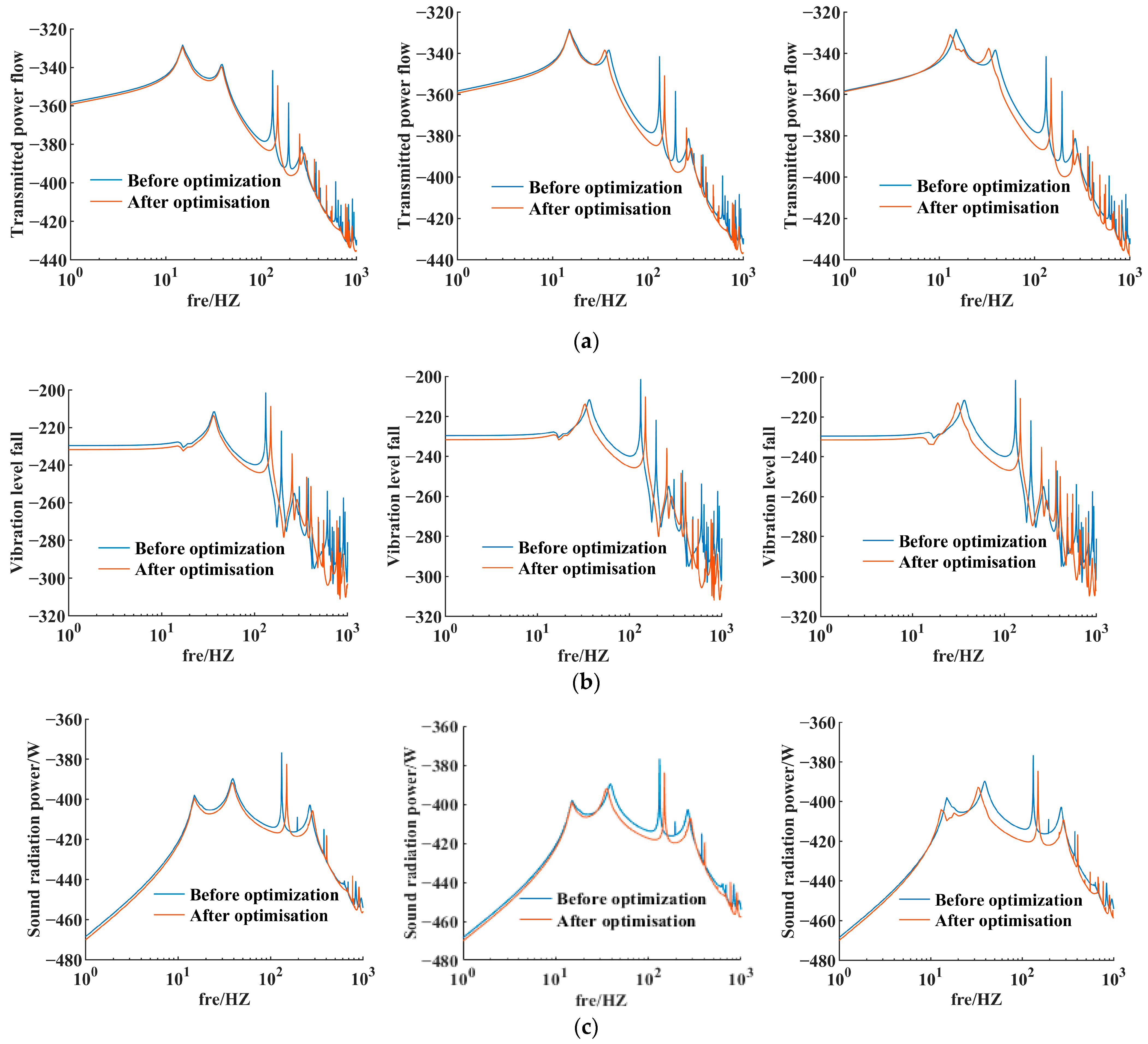
According to the optimized structural parameters shown in Table 5, Table 6 shows the comparison of the magnitude of the root mean square of the objective function before and after the optimization for the coupled system dynamics model, and Figure 11 shows the comparison of the spectra of the coupled system before and after the optimization of the vibration level drop, transferred power flow and acoustic radiated power.
According to the above results, all three methods can achieve optimised results in terms of reduced sound radiated power if the minimum sound radiated power is used as the final evaluation criterion. However, in comparison, method 3 has the best optimisation results followed by method 2, and method 1 has the worst results. There are several reasons for this. The first is that the transmitted power flow has a more direct numerical correspondence with the acoustic radiated power according to the analytical conclusions in Section 3.3. The second is that when combining the transmitted power flow and the vibration level dropout for multi-objective optimisation, on the one hand more optimisation variables are covered, and on the other hand the cross effect between some parameters and multiple objective functions may be more fully represented. For example, in Table 5, the results of method 3 for the raft frame mass mR, the lower vibration isolator stiffness kR, the cylindrical thin shell thickness d, the upper unit 1 mass m1 and the loss factor η of the vibration isolator are geometrically identical to the optimization results when using the transferred power flow or the vibration stage dropout as the objective function alone, but the optimization results of method 3 for the upper vibration isolator stiffness k2 and the lower vibration isolator spacing Hx differ significantly from those of methods 1 and 2, especially when Hx is used as the optimization variable for methods 1, 2 and 3 at the same time, where the optimization results with the vibration level dropout or the transferred power flow as the results of the optimization with a single objective function are roughly the same, while the results of the multi-objective optimization with the vibration level drop and the transferred power flow are significantly different.
5. Conclusions
In this paper, the derivation of the derivative function of a thin submerged cylindrical shell is carried out by combining the plate and shell vibration equation with the Helmholtz equation, and the dynamics model of a thin submerged cylindrical shell containing a complex internal elastic coupling system is established by using the integrated derivative method. On the basis of the above work, the global sensitivity analysis of the dynamic parameters in the frequency domain is carried out using the Sobol’s exponent method with the transfer power flow, vibration level dropout and acoustic radiation power of the coupled system as the objective functions, and the optimization strategy of the dynamic structure parameters based on the transfer power flow, vibration level dropout and transfer power flow + vibration level dropout as the objective functions is discussed accordingly. The main findings of the study are as follows.
- (1)
- The radiation sound field distribution of the coupled system, including sound pressure directivity and main flap amplitude, shows a more complex variation pattern with frequency, which is related to the vibration mode of the coupled system, among which in the low frequency band where the sound pressure amplitude is large, the main flap of sound pressure mainly appears in the direction of excitation force action as well as the direction perpendicular to the excitation force.
- (2)
- On the whole, the ratio curve between the transmitted power flow and the vibration level dropout (difference in decibels) has a relatively regular linear or nearly linear nature, and the ratio between the acoustic radiated power and the transmitted power flow (ratio of decibels) grows approximately linearly in the lower frequency band and tends to 1 in the higher frequency band. However, it must be noted that in the resonance region of the coupled system, the above ratio will show large fluctuations.
- (3)
- The sensitivity analysis of the parameters with greater and lesser influence on the vibroacoustic transmission shows that the parameters of the vibration isolator and the impedance characteristics of the receptor have a significant influence in the low frequency range, while in the higher frequency range, the impedance characteristics of the receptor become the main influencing factor; the variation of the impedance characteristics of the receptor may also make the installation layout of certain vibration isolators on the receptor structure have an important influence on the vibroacoustic transmission characteristics. In addition, this paper also shows that the sensitivity calculation results of the vibration level dropout and the acoustic radiated power seem to have a high similarity.
- (4)
- Use the transferred power flow and the vibration level dropout as objective functions can effectively optimise the acoustic radiation index of the coupled system. At the same time, the ranking of the acoustic radiation optimisation effect is greater when the transferred power flow and the level drop are used as the same objective function than when the transferred power flow is used as the objective function than when the level drop is used as the objective function.
Author Contributions
Conceptualization, S.L., R.H. and L.W.; methodology, S.L., R.H. and L.W.; software, S.L. and L.W.; validation, S.L. and L.W.; investigation, S.L. and R.H.; data curation, S.L., R.H. and L.W.; writing—original draft preparation, S.L. and L.W.; writing—review and editing, S.L., R.H. and L.W.; visualization, S.L.; supervision, R.H.; project administration, R.H.; funding acquisition, R.H. All authors have read and agreed to the published version of the manuscript.
Funding
This research received no external funding.
Institutional Review Board Statement
Not applicable.
Informed Consent Statement
Not applicable.
Data Availability Statement
The data used to support the findings of this study are available from the corresponding authors upon request.
Conflicts of Interest
The authors declare no conflict of interest.
References
- Zhang, L.; Li, B.; Yang, Z.C.; Lu, Y.D. Research on coupling noise source identification and spatial acoustic field localization of an underwater cylindrical cabin model. J. Ship Mech. 2021, 25, 238–245. [Google Scholar]
- Peng, C.G.; Zhang, S.Y.; Zhang, G.J. Study on acoustic vibration similarity law of complex stiffened cone-cylinder combined shell. J. Ship Res. 2022, 17, 165–172. [Google Scholar]
- Li, K.; Yu, M.S. Vibro-acoustic coupling analysis of deepsubmerged spherical shells. J. Ship Mech. 2022, 26, 584–594. [Google Scholar]
- Meyer, V.; Maxit, L.; Guyader, J.L.; Leissing, T. Prediction of the vibroacoustic behavior of a submerged shell with non-axisymmetric internal substructures by a condensed transfer function method. J. Sound Vib. 2016, 360, 260–276. [Google Scholar] [CrossRef] [Green Version]
- Meyer, V. Development of a Substructuring Approach to Model the Vibroacoustic Behavior of Submerged Stiffened Cylindrical Shells Coupled to Non-Axisymmetric Internal Frames. Ph.D. Thesis, Université de Lyon, Lyon, France, 2016. [Google Scholar]
- Cao, X.T. Acoustic radiation from stiffened double concentric large cylindrical shells: Part I Circumferential harmonic waves. J. Vib. Acoust. 2023, 145, 1–44. [Google Scholar] [CrossRef]
- Li, C.H. Prediction of Ship Equipment Vibration Transmission and Study on Vibration Isolation Effect of Floating Raft. Master’s Thesis, Harbin Institute of Technology, Harbin, China, 2016. [Google Scholar]
- Sun, H.L. Simplified performance indicators and active control force of vibration isolation systems with elastic base. Acta Acust. 2016, 41, 227–235. [Google Scholar]
- Zheng, Q.; Lv, Z.Q.; Shuai, C.G.; Li, Y. Research on transmission characteristics of power flow in single stage vibration isolation system on flexible base. Ship Sci. Technol. 2017, 39, 64–68. [Google Scholar]
- Sun, Y.; Yang, T.J.; Liang, W.L.; Chen, B.; Huang, D. Vibration and sound radiation from a flexible base excited by a complex vibration isolation structure. J. Vib. Eng. Technol. 2015, 28, 902–909. [Google Scholar]
- Sun, Y. Research on Sound Radiation from the Flexible Base of a Vibration Isolation System and Its Active Control. Ph.D. Thesis, Harbin Engineering University, Harbin, China, 2016. [Google Scholar]
- Ma, Y.Z. Power Flow Transmission Analysis of Nonlinear Isolation System Based on Flexible Foundation. Master’s Thesis, Shandong University, Jinan, China, 2008. [Google Scholar]
- Randin, D.; Abakumov, A.; Goryachkin, A. Research of a Nonlinear Vibration Isolation System with a Controlled Magnetorheological Damper. In Proceedings of the 7th International Conference on Industrial Engineering London, London, UK, 7–9 July 2021. [Google Scholar]
- Park, Y.H.; Kwon, S.C.; Koo, K.R.; Oh, H.U. High damping passive launch vibration isolation system using superelastic SMA with multilayered viscous lamina. Aerospace 2021, 8, 201. [Google Scholar] [CrossRef]
- Nazeer, A.; Nair, R.P.; Ebenezer, D.D. Numerical Analysis of a Vibration Isolator under Shock Load. In Recent Advances in Applied Mechanics: Proceedings of Virtual Seminar on Applied Mechanics; Springer: Singapore, 2022. [Google Scholar]
- Dalela, S.; Balaji, P.S.; Jena, D.P. Design of a metastructure for vibration isolation with quasi-zero-stiffness characteristics using bistable curved beam. Nonlinear Dyn. 2022, 108, 1931–1971. [Google Scholar] [CrossRef]
- Saffari, P.R.; Sirimontree, S.; Thongchom, C.; Jearsiripongkul, T.; Saffari, P.R.; Keawsawasvong, S. Effect of uniform and nonuniform temperature distributions on sound transmission loss of double-walled porous functionally graded magneto-electro-elastic sandwich plates with subsonic external flow. Int. J. Thermofluids 2023, 17, 100311. [Google Scholar] [CrossRef]
- Sobol’, I.M. Sensitivity estimates for nonlinear mathe2matical model. Appl. Math. Comput. 1993, 55, 407–414. [Google Scholar]
- Sobol’, I.M. On quasi-Monte Carlo integrations. Math. Comput. Simul. 1998, 47, 103–112. [Google Scholar] [CrossRef]
- Sobol’, I.M.; Levitan, Y.L. On the use of variance reducing multipliers in Monte Carlo computations of a global sensitivity index. Comput. Phys. Commun. 1999, 117, 52–61. [Google Scholar] [CrossRef]
- Cai, Q. Research on the Optimization Method of Mixed-Mode Magnetorheological Suspension Structure Based on the Whole Vehicle Model. Master’s Thesis, Chongqing Jiaotong University, Chongqing, China, 2021. [Google Scholar]
- Yang, Q.H. Multi-Mode Magnetorheological Suspension Structure Multi-Objective Optimization Based on Whole Vehicle Vibration Control. Master’s Thesis, Chongqing Jiaotong University, Chongqing, China, 2020. [Google Scholar]
- Du, H.Y.; Li, H.G.; Meng, G.; Fu, X.H. Modeling analysis and structural optimization of horizontal sliding table for ultra-large electromagnetic vibration test equipment. J. Vib. Shock. 2021, 40, 305–312. [Google Scholar]
- Li, R. Study on the Application of Sobol’ Sensitivity Analysis Method in the Analysis of Dynamic Properties of Structures. Master’s Thesis, Hunan University, Changsha, China, 2003. [Google Scholar]
- He, Z.Y. Structural Vibration and Sound Radiation, 1st ed.; Harbin University of Engineering Press: Harbin, China, 2001; pp. 117–122. [Google Scholar]
- Ma, D.Y. Foundations of Modern Acoustic Theory, 1st ed.; Science Press: Beijing, China, 2004; pp. 95–96. [Google Scholar]
Figure 1.
Coupling system diagram: (a) 3D view of the system (b) x direction; (c) z direction.
Figure 2.
Power transfer relationship between mechanical equipment and ship body coupling system.
Figure 3.
Example of calculation results for the vertical conductor.
Figure 4.
Comparison of finite element method and Parsing solution: (a) observation points P0; (b) observation points P1; (c) observation points P2.
Figure 4.
Comparison of finite element method and Parsing solution: (a) observation points P0; (b) observation points P1; (c) observation points P2.
Figure 5.
Pattern of sound pressure distribution: (a–c) Sound pressure for different frequencies; (d) Sound pressure for different axial distances; (e) Sound pressure for different radial distances.
Figure 5.
Pattern of sound pressure distribution: (a–c) Sound pressure for different frequencies; (d) Sound pressure for different axial distances; (e) Sound pressure for different radial distances.
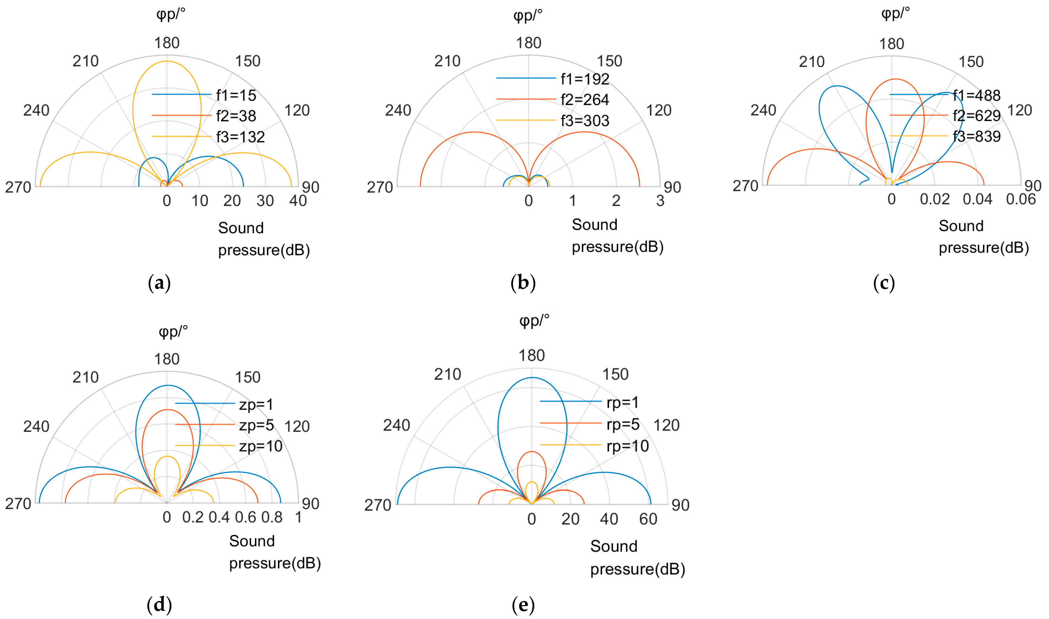
Figure 6.
Comparison of vibration level dropout with Transmitted power flow: (a) Condition 1; (b) Condition 2; (c) Condition 3.
Figure 6.
Comparison of vibration level dropout with Transmitted power flow: (a) Condition 1; (b) Condition 2; (c) Condition 3.

Figure 7.
Comparison of transmitted power flow with water sound pressure and sound radiated power: (a) Condition 1; (b) Condition 2; (c) Condition 3.
Figure 7.
Comparison of transmitted power flow with water sound pressure and sound radiated power: (a) Condition 1; (b) Condition 2; (c) Condition 3.
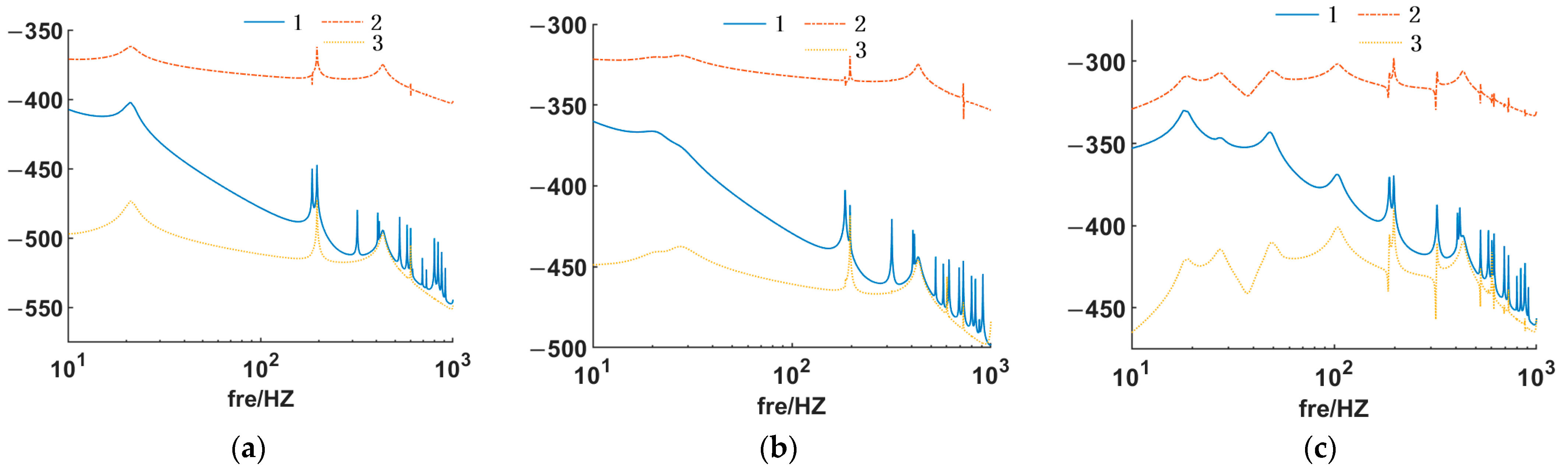
Figure 8.
Ratio between transmitted power flow, sound pressure, and sound radiated power: (a) Condition 1; (b) Condition 2; (c) Condition 3.
Figure 8.
Ratio between transmitted power flow, sound pressure, and sound radiated power: (a) Condition 1; (b) Condition 2; (c) Condition 3.
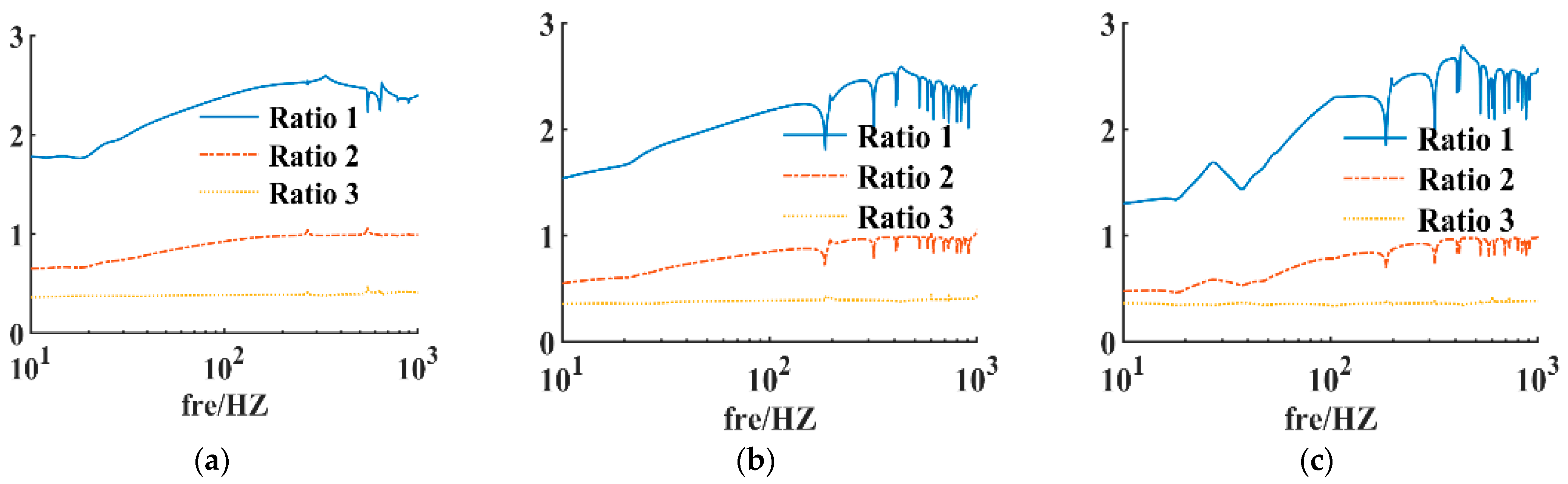
Figure 9.
Ratio between vibration level dropout and transmitted power flow.

Figure 10.
Global sensitivity analysis for each frequency band parameter: (a–c) Sensitivity analysis of power flow, vibration level drop and acoustic radiation power in 15 Hz; (d–f) Sensitivity analysis of power flow, vibration level drop and acoustic radiation power in 38 Hz; (g–i) Sensitivity analysis of power flow, vibration level drop and acoustic radiation power in 132 Hz; (j–l) Sensitivity analysis of power flow, vibration level drop and acoustic radiation power in 194 Hz; (m–o) Sensitivity analysis of power flow, vibration level drop and acoustic radiation power in 264 Hz.

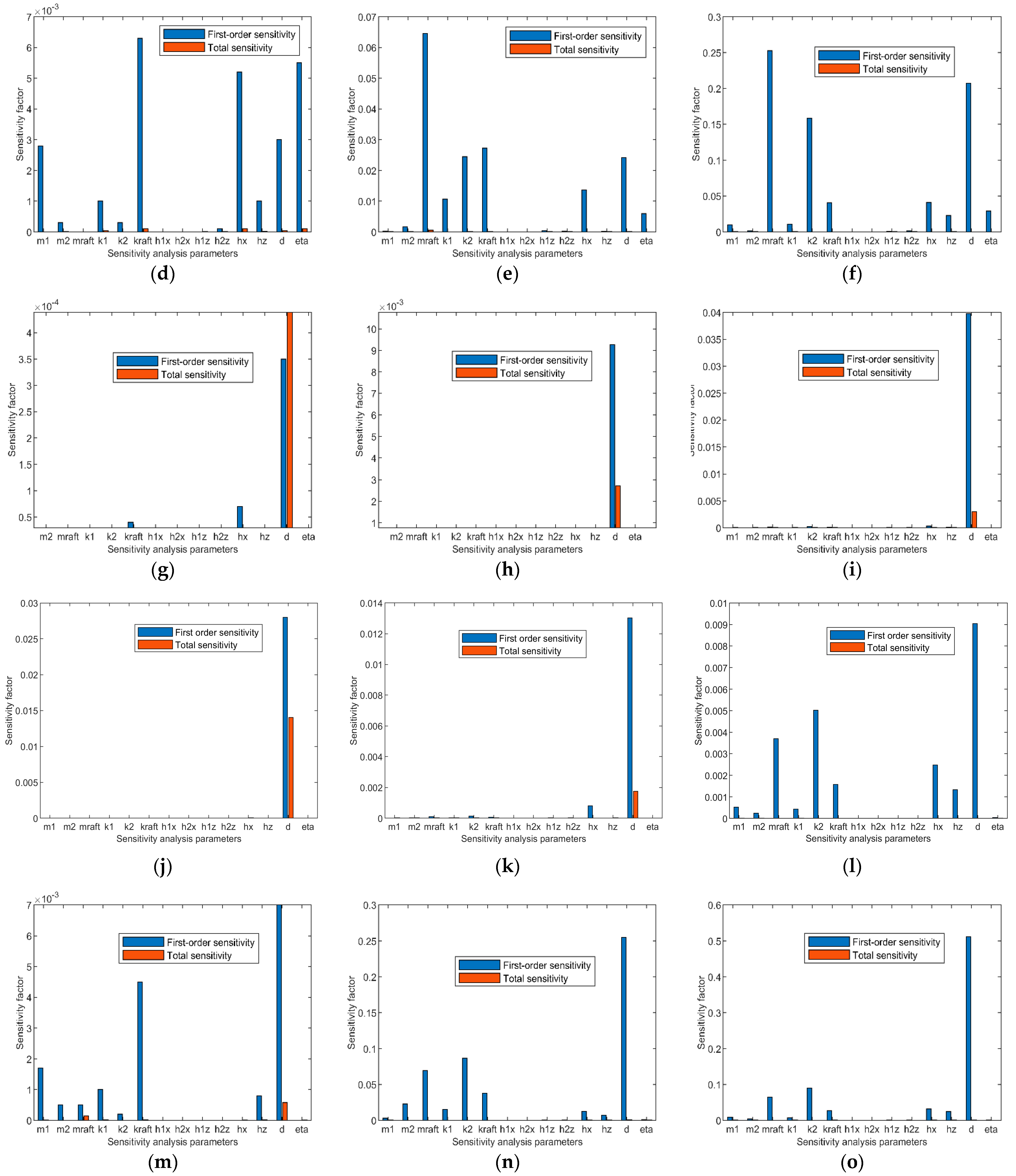
Figure 11.
Optimisation results for coupled systems: (a) Optimisation results for transferring power flows by method 1, 2 and 3; (b) Optimisation results for vibration level drop by method 1, 2 and 3; (c) Optimisation results for acoustic radiation by method 1, 2 and 3.
Figure 11.
Optimisation results for coupled systems: (a) Optimisation results for transferring power flows by method 1, 2 and 3; (b) Optimisation results for vibration level drop by method 1, 2 and 3; (c) Optimisation results for acoustic radiation by method 1, 2 and 3.

Table 1.
Parameters of generator set, raft rack and vibration isolator.
| Parameters | Unit | Condition 1 | Condition 2 | Condition 3 |
|---|---|---|---|---|
| Unit quality m1, m2 | kg | 50, 70 | 100, 140 | 150, 210 |
| Upper vibration isolator re-stiffening k1, k2 | N/m2 | 10 × 105 × (1 + 0.1j) 1 × 105 × (1 + 0.1) | 2 × 105 × (1 + 0.2j) 2 × 105 × (1 + 0.2j) | 1.3 × 106 × (1 + 0.15j) 1.3 × 106 × (1 + 0.15j) |
| Upper vibration isolator spacing h1x, h1z, h2x, h2z | m | 0.06, 0.1, 0.06, 0.1 | 0.1, 0.15, 0.1, 0.15 | 0.2, 0.3, 0.2, 0.3 |
| Lower vibration isolator stiffness kR | N/m2 | 1 × 105 × (1 + 0.1j) | 2 × 105 × (1 + 0.2j) | 2.6 × 106 × (1 + 0.15j) |
| Lower vibration isolator spacing Hx, Hz | m | 0.18, 0.35 | 0.36, 0.7 | 0.5, 1.05 |
| Raft frame quality mR | kg | 100 | 200 | 300 |
| Rotational inertia of unit 1 Jx | Kg·m2 | 1 | 1 | 1 |
| Rotational inertia of unit 2 Jz | Kg·m2 | 1 | 1 | 1 |
| Inertia of raft frame rotation JRx | Kg·m2 | 1 | 1 | 1 |
| Inertia of raft frame rotation JRz | Kg·m2 | 1 | 1 | 1 |
Table 2.
Range of values for sensitivity analysis of coupled vibration system parameters.
| Names and Symbols | Mean Value of Parameters (μ) | Variance (σ) | Range of Variations |
|---|---|---|---|
| Unit quality m1 | 46 | 0.46 | μ ± 3σ |
| Unit quality m2 | 70 | 0.7 | μ ± 3σ |
| Raft frame quality mR | 100 | 1 | μ ± 3σ |
| Upper vibration isolator stiffness k1 | 2× 105 × (1 + 0.1j) | (1 + 0.1j) × 103 | μ ± 3σ |
| Upper vibration isolator stiffness k2 | 2.7× 105 × (1 + 0.1j) | (1 + 0.1 j) × 103 | μ ± 3σ |
| Lower vibration isolator stiffness kR | 8.6× 105 × (1 + 0.1j) | (1 + 0.1 j) × 103 | μ ± 3σ |
| Upper vibration isolator spacing h1x | 0.2 | 0.002 | μ ± 3σ |
| Upper vibration isolator spacing h1z | 0.2 | 0.002 | μ ± 3σ |
| Upper vibration isolator spacing h2x | 0.3 | 0.003 | μ ± 3σ |
| Upper vibration isolator spacing h2z | 0.3 | 0.003 | μ ± 3σ |
| Lower vibration isolator spacing Hx | 0.35 | 0.0035 | μ ± 3σ |
| Lower vibration isolator spacing Hz | 0.7 | 0.007 | μ ± 3σ |
| Cylindrical thin shell thickness d | 0.02 | 0.0002 | μ ± 3σ |
| Vibration isolator loss factor η | 0.1 | 0.001 | μ ± 3σ |
Table 3.
Planning models.
| Method 1 | Method 2 | Method 3 | |
|---|---|---|---|
| Objective functions | |||
| Binding conditions |
Table 4.
Range of values for the design variables of the coupled system parameters optimization.
| Names and Symbols | Mean Value of Parameters | Variance | Range of Variations |
|---|---|---|---|
| Mass of upper unit m1 | 46 | 0.46 | μ ± 30σ |
| Raft frame quality mR | 100 | 1 | μ ± 30σ |
| Stiffness of upper vibration isolators k2 | 2.7 × 105 × (1 + 0.1j) | 2.7 × 103 × (1 + 0.1j) | μ ± 30σ |
| Stiffness of the lower vibration isolator kR | 8.6 × 105 × (1 + 0.1j) | 8.6 × 103 × (1 + 0.1j) | μ ± 30σ |
| Spacing of lower vibration isolators Hx | 0.35 | 0.0035 | μ ± 30σ |
| Thickness of cylindrical thin shells d | 0.02 | 0.0002 | μ ± 30σ |
| Loss factor for vibration isolators η | 0.1 | 0.001 | μ ± 30σ |
Table 5.
Comparison of coupling system parameters before and after optimization.
| Names and Symbols | Values before Optimisation | Optimisation (Method 1) | Optimisation (Method 2) | Optimisation (Method 3) |
|---|---|---|---|---|
| Mass of upper unit m1 | 46.0 | 47.32 | \ | 47.32 |
| Raft frame quality mR | 100 | \ | 127 | 127 |
| Stiffness of upper vibration isolators k2 | 2.70 × 105 × (1 + 0.1j) | \ | 2.84 × 105 × (1 + 0.1j) | 1.80 × 105 × (1 + 0.0996j) |
| Stiffness of the lower vibration isolator kR | 8.60 × 105 × (1 + 0.1j) | 8.32 × 10⁵ (1 + 0.0992j) | \ | 8.32 × 105 × (1 + 0.0996j) |
| Spacing of lower vibration isolators Hx | 0.35 | 0.295 | 0.299 | 0.254 |
| Thickness of cylindrical thin shells d | 0.02 | 0.0254 | 0.0254 | 0.0254 |
| Loss factor for vibration isolators η | 0.10 | 0.0992 | \ | 0.0996 |
Table 6.
Comparison of the objective function before and after optimization for the coupled vibration system.
Table 6.
Comparison of the objective function before and after optimization for the coupled vibration system.
| Names and Symbols | Values before Optimisation | Optimisation (Method 1) | Optimisation (Method 2) | Optimisation (Method 3) |
|---|---|---|---|---|
| transmitted power flow (RMS) | 1.41 × 10⁻⁹ | 8.13 × 10⁻¹⁰ | 1.25 × 10⁻⁹ | 9.68 × 10⁻¹⁰ |
| vibration level dropout (RMS) | 1.45 × 10⁻⁴ | 1.75 × 10⁻⁵ | 1.18 × 10⁻⁵ | 1.77 × 10⁻⁵ |
| acoustic radiated power (RMS) | 9.68 × 10⁻¹³ | 2.95 × 10⁻¹³ | 4.72 × 10⁻¹³ | 1.10 × 10⁻¹³ |
Disclaimer/Publisher’s Note: The statements, opinions and data contained in all publications are solely those of the individual author(s) and contributor(s) and not of MDPI and/or the editor(s). MDPI and/or the editor(s) disclaim responsibility for any injury to people or property resulting from any ideas, methods, instructions or products referred to in the content. |
© 2023 by the authors. Licensee MDPI, Basel, Switzerland. This article is an open access article distributed under the terms and conditions of the Creative Commons Attribution (CC BY) license (https://creativecommons.org/licenses/by/4.0/).
Share and Cite
MDPI and ACS Style
Liu, S.; Huo, R.; Wang, L. Vibroacoustic Transfer Characteristics of Underwater Cylindrical Shells Containing Complex Internal Elastic Coupled Systems. Appl. Sci. 2023, 13, 3994. https://doi.org/10.3390/app13063994
AMA Style
Liu S, Huo R, Wang L. Vibroacoustic Transfer Characteristics of Underwater Cylindrical Shells Containing Complex Internal Elastic Coupled Systems. Applied Sciences. 2023; 13(6):3994. https://doi.org/10.3390/app13063994
Chicago/Turabian StyleLiu, Shuqing, Rui Huo, and Likang Wang. 2023. "Vibroacoustic Transfer Characteristics of Underwater Cylindrical Shells Containing Complex Internal Elastic Coupled Systems" Applied Sciences 13, no. 6: 3994. https://doi.org/10.3390/app13063994
Note that from the first issue of 2016, this journal uses article numbers instead of page numbers. See further details here.