
Railcar Dynamic Response during Braking Maneuvers Based on Frequency Analysis
by

Gerardo Hurtado-Hurtado
1, 
Luis Morales-Velazquez
1,
Frank Otremba
2 and
Juan C. Jáuregui-Correa
3,* 1
Faculty of Engineering, Autonomous University of Queretaro, Campus San Juan del Río, San Juan del Rio 76807, Mexico
2
Federal Institute for Materials Research and Testing (BAM), 12489 Berlin, Germany
3
Faculty of Engineering, Autonomous University of Queretaro, Santiago de Queretaro 76010, Mexico
*
Author to whom correspondence should be addressed.
Appl. Sci. 2023, 13(7), 4132; https://doi.org/10.3390/app13074132
Submission received: 20 February 2023
/
Revised: 22 March 2023
/
Accepted: 22 March 2023
/
Published: 24 March 2023
(This article belongs to the Special Issue Recent Advances in Vehicle-Track-Ground Coupling Dynamics and Railway-Induced Ground Vibration)
Abstract
:The dynamic response of a vehicle during braking is influenced by the tangential forces developed at the wheel-rail’s contact surface. The friction coefficient affects the load transfer from the wheel’s tread to the vehicle. In this work, the vibrations of a scale-down railway vehicle are monitored during braking and their relationship with the friction coefficient between wheel and rail is found out. The vehicle is instrumented with encoders, accelerometers, and is controlled via Bluetooth. The tests are carried out with clean and friction-modified rails. The tangential forces transmitted from the wheel to the railcar’s body are visualized in time and frequency using a proposed correlation algorithm based on the outputs of the Continuous Wavelet Transform (CWT). The results demonstrate that tangential forces have a significant impact on railway vehicles under conditions of high friction coefficients and large creep values.
1. Introduction
During braking, tangential forces developed in the wheel-rail contact area have a direct effect on the dynamic response of the railway vehicle. As a result, the vehicle’s dynamic response exhibits different frequencies depending on the friction coefficient. Large tangential forces may threaten the stability of the railway vehicles if the braking torque is not applied properly [1], and even damage the train’s wheels, engine, and rails, if applied abruptly [2].
If vibrations caused by braking are very strong, they can be transferred to the vehicle’s body. Railway vehicle vibrations can cause discomfort to passengers and even cause harmful vibrations in railway structures [3]. Koç [4] addresses this issue by proposing a linear actuator adapted to the secondary suspension to reduce vibrations caused by the train-bridge interaction.
Vibration monitoring is used to find faults in railway components. Accelerometers were installed on the axle-box and bogie by Lee et al. [5] to detect lateral and vertical track irregularities. Tsunashima [6] uses a machine-learning-based algorithm to classify rail failures as either vertical, lateral alignment, or cross-level. Wei et al. [7] installed accelerometers on the vehicle bogies to monitor lateral and vertical vibrations, thereby determining track alignment. Jauregui et al. [8] used a technique based on empirical mode decomposition (EMD) to find a transfer function, which converts vehicle accelerations into track deformations. Their proposal aims to visualize the evolution of damage in the track and substructures.
The rolling tangential forces that cause vibrations to the vehicle are generated in a relatively small contact area (ellipse-shape) of 1 cm2 size [9]. The contact area is separated into traction and sliding regions. The ratio between these two regions determines the overall dynamic behavior of the wheel and is dependent on a number of factors, including the coefficient of friction, creep, and the lateral position of the wheel in relation to the rail. As with out-of-round wheels [10,11,12] and rail corrugations [13], the behavior of tangential forces can be monitored from the vehicle’s body using in-service-vehicle devices, with remarkably promising results. Applying the same principle, vibration analysis may detect changes in the wheel-rail friction coefficient.
Wheel-rail friction is approximately 0.3 under dry, clean conditions [14]. This value, however, is not constant and depends on the nature of the contaminants on the rails. Some common contaminants are water, snow, leaves, and even grease. Since the rails and wheels are exposed to the outside environment, it is impossible to maintain ideal friction conditions for optimal performance. In this case, friction modifiers are needed to improve traction when starting off is difficult due to contaminants on rails [15].
Friction modifiers have been studied by many researchers to find the best performance on wheel traction [16,17,18]. It has been reported that the increase in the friction coefficient results in an improvement in the dynamic performance of the locomotives. On the other hand, it has been observed that the rear wheels have better traction because the front wheels sweep away some of the dirt from the track [19]. However, this only improves the performance of the rear wheels by 20%, compared to 32% when friction modifiers such as sand dust are used. Therefore, friction modifiers are preferred to improve acceleration or braking, and even to prevent skidding on hills.
Vibrations are utilized in the aforementioned works in order to identify track anomalies; however, none of these studies have performed vibration analysis in order to identify variations in the coefficient of friction. This paper proves how varying the wheel-rail friction coefficient affects the dynamic response of railway vehicles during braking. The experimental data from a 1:20 scale-down railcar is used for studying the effects of severe braking. The railcar performs braking maneuvers on a straight track with clean rails and friction-modified rails. The vibrations are monitored using accelerometers on the body of the vehicle. In order to compute the slide during braking, the traction wheel speed is measured with a rotary encoder, while the vehicle speed is measured with an optical sensor. Both the traction wheel’s rotary encoder signal and the railcar’s body accelerometer signal are analyzed in the frequency domain to find out how the increase in the friction coefficient affects the vehicle dynamics. A proposed correlation method is used to compare the signals and determine under which conditions the tangential forces are most strongly transmitted to the railcar. The findings show that vibrations from a railway vehicle can be used to investigate the friction coefficient and the tangential forces acting on the wheel tread, providing experts in railway vehicle braking control with the option to consider vibrations to improve braking and acceleration performance.
2. Materials and Methods
The testing vehicle, shown in Figure 1, is a 1:20 model railcar that runs on a straight track. The vehicle consists of a single railcar supported by two bogies, with the rear bogie providing torque and traction. On clean tracks, the vehicle, which is propelled by a servomotor coupled to the traction axle via belt drive, may attain a maximum speed of 1.3 m/s in three seconds. The track rails are round-profile wires with a 5 mm diameter. The body of the railcar is supported by a rigid 8-spring suspension. For optimal transmission and detection of tangential wheel forces on the vehicle’s body, stiff springs are preferred in the suspension. According to impact tests, the damping coefficient is 306 N s/m. The main parameters of the scale-down vehicle are summarized in Table 1.
The frame of the experimental vehicle is constructed primarily of aluminum and the rails are steel. The rails are glued to sleepers that have been machined from a plywood plate. Figure 2 shows a picture of the model on the test bench.
2.1. Experiment Description
The test consists of accelerating the vehicle to its top speed and then abruptly stopping it. At all times, the vehicle velocity, the wheelset velocity, the current, and the railcar’s body acceleration are recorded. Experiments are conducted using both clean and sand-scattered rails to compare the effects of each condition. In the sand-scattered rails test, the entire length of both rails has been covered in a fine layer of sand dust, see Figure 3. Rails that are covered in sand have a friction coefficient of 0.45, while rails that have been thoroughly cleaned have a friction coefficient of 0.2. The static coefficient of friction was calculated using the formula below:
where P is the total vehicle weight and Ff is the static friction force. The force Ff was determined using a spring dynamometer to pull the vehicle along the track with the traction wheel locked.
2.2. Data Adquisition System
The vehicle’s monitoring and control system includes an FPGA board, sensors, and a servomotor. The FPGA board receives instructions and configurations from a Bluetooth module to control the vehicle’s speed and stores the data on a micro-SD card. The control box holds the accelerometers in the middle of the vehicle.
The servomotor, installed on the traction bogie and coupled to the wheelset, applies torque to the traction wheelset to accelerate the vehicle. The servomotor consists of a 12 V brushed DC gearmotor with a metal spur gearbox. The speed of the vehicle is measured by an optical infrared sensor, installed on the trail bogie, and a black-and-white stripe. The wheelset speed is monitored by means of a 600-pulse-per-revolution incremental rotary encoder attached to the wheelset axle by a timing belt, see Figure 4. The current consumption is monitored by a sensor wired into the power input of the motor driver. A 14.8 V Li-Po battery supplies energy for the whole setup. Figure 5 depicts the whole control system diagram.
3. Methodology
The vibration signals are analyzed using the techniques described in this section. Every experiment evaluates four signals: longitudinal (ax), lateral (ay), and vertical (az) railcar acceleration, and wheelset speed (ws). The signals are evaluated to determine if there is a correlation between the wheel’s and vehicle’s dynamics responses.
The vehicle dynamics signal is derived from the vehicle’s body accelerometer. On the other hand, variations in the friction force influence the traction wheelset dynamics, and its behavior can be tracked via the rotary encoder joined to the wheelset axle. Figure 6 illustrates the development of wheel-rail tangential forces.
3.1. Frequency Analysis
The results of the frequency analysis may be distorted due to the presence of very low frequency components inside the processed signals. These components are referred to as rigid-body modes. In order to get rid of the rigid-body modes that are inherent to the vibration waves, the Empirical Mode Decomposition (EMD) is first applied to each signal. Finally, the Fast Fourier Transform (FFT) and the Continuous Wavelet Transform (CWT) are applied to the signals to extract the frequency components and the timings at which they occur, as shown in the flowchart in Figure 7.
FFT is a widely used technique for determining the frequency components of sinusoidal signals. Similarly, the CWT is a method used to determine the frequencies of a signal, as well as their position in time. FFT is used here to investigate the impact of the two different coefficients of friction on the vehicle’s modes and to determine which frequencies are shared by both signals. In addition, the CWT results are used to analyze the evolution of this phenomenon during braking by observing the frequencies over time. Moreover, a time-frequency cross-correlation plot is generated from the wheel and vehicle CWT results for further analysis. The Morlet wavelet is preferred for the CWT, as it is well-suited for evaluating dynamic phenomena [20].
3.2. Correlation Method
The proposed approach makes it possible to see when the tangential forces are transferred from the wheels to the vehicle. The outputs of the CWT applied to the wheel and vehicle vibration signals are used to look for a similarity in frequencies over time.
The CWT results are presented in a matrix format, similar to an image, with the highlighted regions representing the frequencies present in the signal over time. Each of the matrix’s elements is a coefficient whose value indicates whether or not a signal contains specific frequency components. In the spectrogram, the vertical displacement indicates the frequency value, while the horizontal displacement indicates the time at which the frequency appears in the signal.
Figure 8 illustrates the process by simulating some frequencies detected at times t1 and t2. Each of the acceleration images overlaps with the image of the wheelset, and only the areas where both images overlap remain. The final image is the correlation between the two input images. If the CWT image of the wheel closely matches that of the vehicle, this indicates that the vehicle is being affected by tangential forces. The intensity of the vibrations is represented by the coefficients of the final image.
The CWT results of the wheel speed are contained in the array E, whose elements are , whereas the acceleration results are contained in the arrays , , and , whose elements are , , and , respectively. To only consider the highest frequency peaks, an intermediate operation is needed. To accomplish this, we only take into account values that are bigger than a predetermined limit. Therefore, the following conditions apply:
where , , , and are the limit values of the correlation threshold. The elements of the correlation matrixes are then:
The correlation of both signals in frequency and time is given in the set of elements , , and , whose values are different from zero.
4. Results
The results shown here are the FFT spectrum, the CWT spectrograms, and the correlation of the signals of the wheelset speed and the vehicle body accelerations , , and . Each signal is analyzed before and during braking. To avoid other track disturbances like rail joints, the slip zone for vibration analysis was carefully chosen.
4.1. Creep
According to [21], creep is defined as wheel slip in relation to the speed of the vehicle. In this study, longitudinal creep is measured using the vehicle speed and the traction wheel speed signals. The braking of the vehicle and the wheel is depicted in Figure 9 for both tests, which were conducted on clean rails and sand-covered rails. In the case of a clean rail, the vehicle’s braking time is approximately two seconds, whereas sand significantly reduces this time (0.75 s).
In both instances, the slope of the vehicle’s deceleration (red line) is uniform and nearly constant, whereas the deceleration of the wheels (blue line) changes abruptly and remains constant for a while. This difference in speed behavior between the wheel and the vehicle is referred to as slippage. The red line oscillates at high frequencies in both situations, but the effect is more pronounced when sand is present on the rails. These oscillations are a result of the traction wheel’s dynamics.
Figure 10 depicts the clean rail and sand-covered creep curves obtained by:
where is the vehicle’s speed. The clean rail creep curve has the greatest slip (around 85 percent at its peak) and lasts up to 1.5 s. The duration of the sand-covered rail creep curve is only 0.45 s, and its maximum value is only 66%. As was to be expected, the sand, which provides the rail with higher friction, does not permit much slippage and consequently slows down the wheel and the vehicle more rapidly.
4.2. Frequency Analisys before Braking
In the frequency analysis, the methods described in Section 3 are applied to analyze the wheel’s and the railcar’s vibration signals in order to find a similarity between the wheel’s and vehicle’s dynamics. Time and frequency correlations indicate that tangential forces from the wheel are affecting the vehicle.
With the oscillations that appear in the wheel’s speed signal, it is possible to analyze the dynamics of the wheel throughout the entire vehicle’s journey. In this study, the CWT is applied to the wheel encoder signal to determine which frequencies are present during the course.
In this section, the results of a test that were conducted during normal operation (without applying the brakes) are presented. These results can be compared with the results of the braking tests, which are discussed in the following section. The frequencies depicted in the CWT spectrogram in Figure 11 correspond to the wheel’s dynamics prior to braking on a clean rail. The spectrogram is drawn using the elements that result from applying the CWT to . It can be observed that the predominant vibrations (brightest areas) oscillate between 120 and 200 Hz, but only for brief instants. Some of the frequencies found in this analysis relate to the wheel rolling (46 Hz) and the passage of sleepers (25 Hz). The frequencies of the system are summarized in Table 2.
Figure 11 also depicts the frequency spectrum determined by FFT of the same signal in the same time interval. The peaks in this spectrum that are enclosed in black squares represent frequencies that are also present in the railcar accelerometer signals, as will be demonstrated in the following lines.
Figure 12 depicts the FFT spectrum of the vehicle’s body vibrations, which also exhibits very active dynamics; these results come from the same window of time as Figure 11. According to Figure 11 and Figure 12, wheel and vehicle share a number of frequencies, including 66, 87, 132, 154, and 197 Hz. The spectrogram illustrates how these frequencies can also be visualized in time by using the results , , and . However, these frequency components do not manifest in all directions, exerting minimal influence only in the lateral and vertical directions, as can be seen in the correlation results. This correlation image was generated utilizing Equations (2) and (3), with , , , and as equal to 1.5 times the mean value from , , , and , respectively. This threshold is used for all correlations in this paper.
Before braking, the wheel dynamics on sand-covered rails differ significantly from those on clean rails. As shown in Figure 13, the amplitudes are diminished and the frequencies appear to be more dispersed. Nonetheless, the detected frequencies are higher (around 168 Hz). This is partially due to the fact that the sand grains are evenly distributed over the rails, causing the wheels to be randomly excited.
During normal operation, the vehicle dynamics on sand-covered rails appear somewhat disorderly, except in the vertical direction where components oscillate around 169 Hz and occasionally approach 100 Hz. Nevertheless, despite the disorder, the frequency of 169 Hz is present in all the signals, as demonstrated by the correlation in Figure 14.
The dynamics on sand-covered rails show numerous matches in the correlation, represented by the coefficients , , and given by Equation (3). This is not, however, convincing proof of similar dynamics, as almost all coincidences occur for a brief instant.
4.3. Frequency Analisys during Braking
The dynamics of the wheel during braking on clean rails (lower coefficient of friction) exhibit less frequency variations and smaller amplitudes than when the vehicle is not braking, as can be seen in Figure 15. This is primarily caused by a significant slide between the wheel and rail; see also Figure 10a.
Low-intensity vehicle dynamics occur while braking on clean rails. A small number of wheel frequencies, including 66 and 152 Hz, are translated to the vehicle’s chassis. Figure 16 demonstrates that the vehicle exhibits the most interesting dynamics in the vertical direction, having few prominent coincidences around 152 Hz. These coincidences take place once the maximum creep rate of 85% is reached in the wheel, see Figure 10a.
When the wheel is forced to brake while running on rails that are covered in sand, its dynamics are completely different from those of any of the previous cases. As shown by the CWT results in Figure 17, the wheel oscillates at approximately 144 Hz throughout this entire region (from t = 0.2 and 0.7 s). Although the vibration amplitudes are not the greatest among all cases, a significant number of vibrations from the traction wheels are also transmitted to the vehicle’s body.
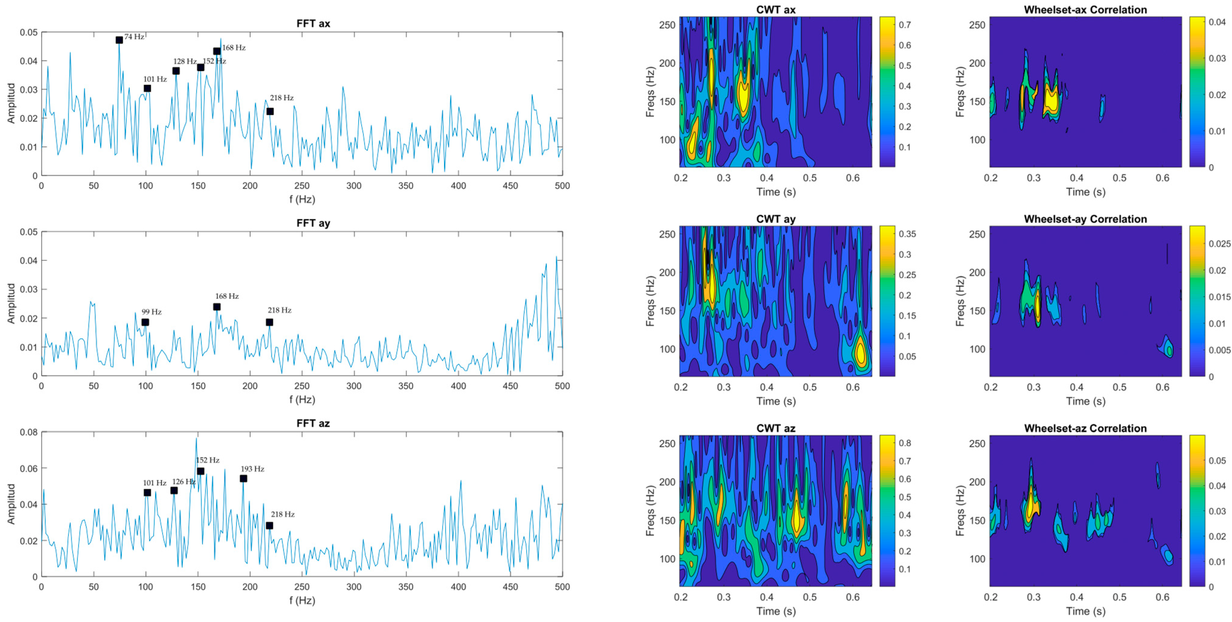
In this test, the vehicle appears to vibrate more intensely in the longitudinal and vertical directions, due to the wheel’s dynamics. Figure 18 illustrates the correlation between wheel and vehicle dynamics, where it is evident that tangential forces have a significant impact on the vehicle response.
5. Conclusions
In this work, a study was carried out on how the change in the wheel-rail friction coefficient affects the vibration behavior of a scale-down railcar during braking tests. The experiments were conducted on clean and sand-scattered rails. Accelerations of the vehicle’s body, current consumption, and traction wheelset speed were all measured. Different coefficients of friction lead to different braking behaviors, as shown by the computed creep in the braking zone. Vibration signals from the traction wheelset dynamics and the vehicle’s body dynamics were analyzed to assess whether the tangential forces are transmitted to the vehicle’s body using FFT and CWT methods and a proposed correlation method.
Due to its speed and accuracy, the FFT is the most popular technique. In this work, the CWT technique stands out the most. Using only the FFT, it is difficult to recognize that something different occurred when the coefficient of friction was increased; however, the CWT spectrograms reveal that the dynamics of the wheel changed drastically when the friction coefficient was increased.
The fact that the dynamics of the vehicle and the traction wheel are similar when increasing the friction coefficient suggests that the tangential forces are strong enough to be observed from the vehicle’s body. The proposed correlation method makes it simple to assess whether or not the two dynamics are similar, providing an invaluable resource for determining under what conditions the coefficient of friction has the greatest impact on railway vehicle dynamics.
The work presented here confirms that variations in the coefficient of friction influence vehicle’s body vibrations. Thus, vibration data collected from the vehicle’s body can be used to detect transitions in the coefficient of friction. The results of this study will be helpful to those investigating railway braking systems by identifying the optimum conditions for braking and accelerating using vibration measurements from the locomotive cab.
It remains a possibility to conduct the same study on actual railway vehicles in order to demonstrate that changes in the coefficient of friction affect the vehicle’s dynamic response.
Author Contributions
Conceptualization, G.H.-H., J.C.J.-C. and F.O.; software, G.H.-H. and L.M.-V.; writing—review and editing, G.H.-H. All authors have read and agreed to the published version of the manuscript.
Funding
This research received no external funding.
Institutional Review Board Statement
Not applicable.
Informed Consent Statement
Not applicable.
Data Availability Statement
The data presented in this study are not publicly available due to privacy issues.
Acknowledgments
The authors would like to thank Consejo Nacional de Ciencia y Tecnología, CONACyT by the Scholarship with key code 2018-000068-02NACF.
Conflicts of Interest
The authors declare no conflict of interest.
References
- Zhang, Z.; Dhanasekar, M. Dynamics of railway wagons subjected to braking/traction torque. Veh. Syst. Dyn. 2009, 47, 285–307. [Google Scholar] [CrossRef]
- Lixin, Q.; Haitao, C. Three dimension dynamics response of car in heavy haul train during braking mode. In Proceedings of the 7th International Heavy Haul Conference, Brisbane, Australia, 10–14 June 2001; pp. 231–238. [Google Scholar]
- Eroğlu, M.; Koç, M.A.; Esen, I.; Kozan, R. Train-structure interaction for high-speed trains using a full 3D train model. J. Braz. Soc. Mech. Sci. Eng. 2022, 44, 1–28. [Google Scholar] [CrossRef]
- Koç, M.A. A new expert system for active vibration control (AVC) for high-speed train moving on a flexible structure and PID optimization using MOGA and NSGA-II algorithms. J. Braz. Soc. Mech. Sci. Eng. 2022, 44, 1–24. [Google Scholar] [CrossRef]
- Lee, J.S.; Choi, S.; Kim, S.-S.; Park, C.; Kim, Y.G. A Mixed Filtering Approach for Track Condition Monitoring Using Accelerometers on the Axle Box and Bogie. IEEE Trans. Instrum. Meas. 2011, 61, 749–758. [Google Scholar] [CrossRef]
- Tsunashima, H. Condition monitoring of railway tracks from car-body vibration using a machine learning technique. Appl. Sci. 2019, 9, 2734. [Google Scholar] [CrossRef] [Green Version]
- Wei, X.; Liu, F.; Jia, L. Urban rail track condition monitoring based on in-service vehicle acceleration measurements. Measurement 2016, 80, 217–228. [Google Scholar] [CrossRef]
- Jauregui-Correa, J.C.; Morales-Velazquez, L.; Otremba, F.; Hurtado-Hurtado, G. Method for predicting dynamic loads for a health monitoring system for subway tracks. Front. Mech. Eng. 2022, 8, 1–16. [Google Scholar] [CrossRef]
- Iwnicki, S.; Iwnicki, S. (Eds.) Tribology of the Wheel-Rail Contact. In Handbook of Railway Vehicle Dynamics, 1st ed.; CRC Press: Boca Raton, FL, USA, 2006; pp. 282–291. [Google Scholar]
- Nielsen, J.C.; Johansson, A. Out-of-round railway wheels-a literature survey. Proc. Inst. Mech. Eng. Part F J. Rail Rapid Transit. 2000, 214, 79–91. [Google Scholar] [CrossRef]
- Tao, G.; Wen, Z.; Liang, X.; Ren, D.; Jin, X. An investigation into the mechanism of the out-of-round wheels of metro train and its mitigation measures. Veh. Syst. Dyn. 2019, 57, 1–16. [Google Scholar] [CrossRef]
- Ye, Y.; Zhu, B.; Huang, P.; Peng, B. OORNet: A deep learning model for on-board condition monitoring and fault diagnosis of out-of-round wheels of high-speed trains. Measurement 2022, 199, 111268. [Google Scholar] [CrossRef]
- Tanaka, H.; Matsumoto, M.; Harada, Y. Application of axle-box acceleration to track condition monitoring for rail corrugation management. In Proceedings of the 7th IET Conference on Railway Condition Monitoring 2016 (RCM 2016), Birmingham, UK, 27–28 September 2016. [Google Scholar] [CrossRef]
- Moore, D.F. Chapter 14—Transportation and Locomotion. In Principles and Applications of Tribology; Elsevier: Amsterdam, The Netherlands, 1975; pp. 302–330. [Google Scholar]
- Harmon, M.; Lewis, R. Review of top of rail friction modifier tribology. Tribol. Mater. Surf. Interfaces 2016, 10, 150–162. [Google Scholar] [CrossRef]
- Lundberg, J.; Rantatalo, M.; Wanhainen, C.; Casselgren, J. Measurements of friction coefficients between rails lubricated with a friction modifier and the wheels of an IORE locomotive during real working conditions. Wear 2015, 324–325, 109–117. [Google Scholar] [CrossRef] [Green Version]
- Lu, X.; Cotter, J.; Eadie, D. Laboratory study of the tribological properties of friction modifier thin films for friction control at the wheel/rail interface. Wear 2005, 259, 1262–1269. [Google Scholar] [CrossRef]
- Arias-Cuevas, O.; Li, Z.; Lewis, R.; Gallardo-Hernandez, E.A. Rolling–sliding laboratory tests of friction modifiers in dry and wet wheel–rail contacts. Wear 2010, 268, 543–551. [Google Scholar] [CrossRef] [Green Version]
- Bosso, N.; Gugliotta, A.; Magelli, M.; Oresta, I.F.; Zampieri, N. Study of wheel-rail adhesion during braking maneuvers. Procedia Struct. Integr. 2019, 24, 680–691. [Google Scholar] [CrossRef]
- Hurtado-Hurtado, G.; Morales-Velazquez, L.; Valtierra-Rodríguez, M.; Otremba, F.; Jáuregui-Correa, J.C. Frequency Analysis of the Railway Track under Loads Caused by the Hunting Phenomenon. Mathematics 2022, 10, 2286. [Google Scholar] [CrossRef]
- Polach, O. Creep forces in simulations of traction vehicles running on adhesion limit. Wear 2005, 258, 992–1000. [Google Scholar] [CrossRef]
Figure 1.
The scaled-down vehicle used in this study. Red fonts: sensors, blue fonts: principal components.
Figure 1.
The scaled-down vehicle used in this study. Red fonts: sensors, blue fonts: principal components.
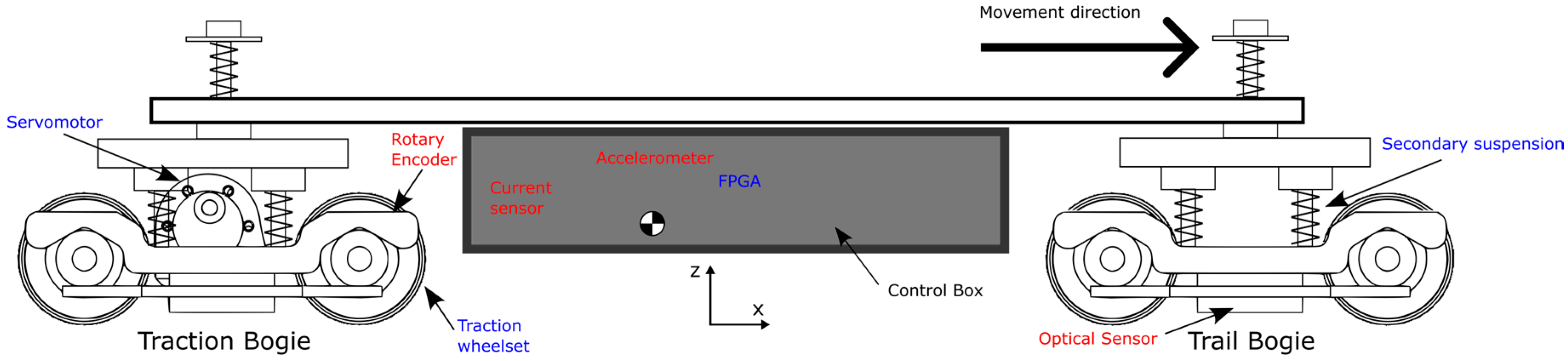
Figure 2.
The experimental vehicle. See Table 1 for the principal parameters.
Figure 2.
The experimental vehicle. See Table 1 for the principal parameters.

Figure 3.
Sand-scattered rails.
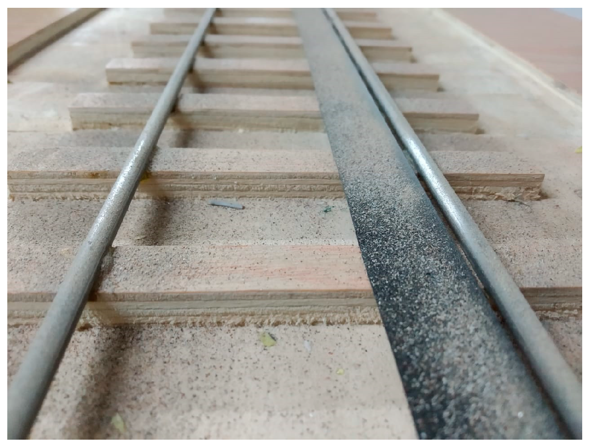
Figure 4.
Traction bogie. The rotary encoder monitors the wheelset speed.
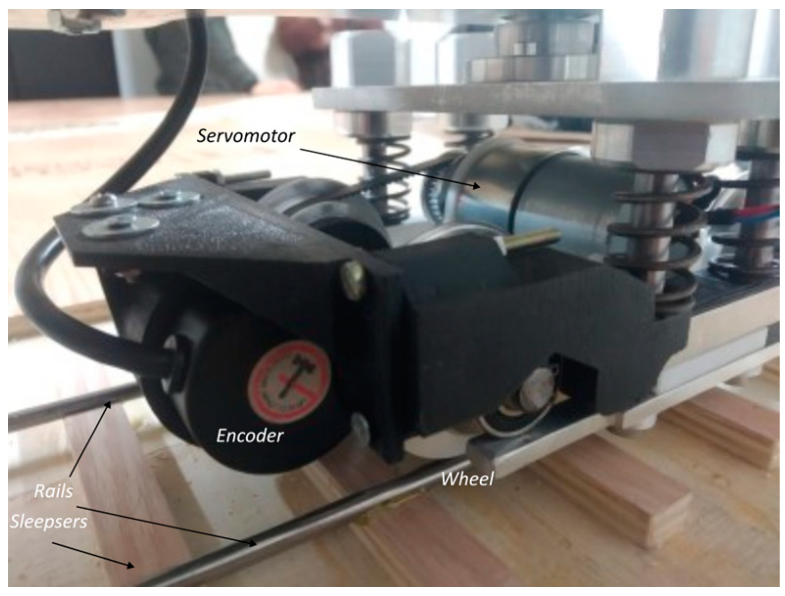
Figure 5.
The control system diagram displaying the different modules connected to the control board.
Figure 5.
The control system diagram displaying the different modules connected to the control board.

Figure 6.
The development of tangential forces at the wheel-rail contact surfaces during acceleration. The weight P of the entire vehicle is supported by all eight wheels; therefore, the drive wheels each support 1/8 of the total weight. By means of a torque T and an angular velocity ω, the wheel exerts a traction force FT tangentially on the rail surface. The frictional force Ff has the same magnitude as FT, but acts in the opposite direction. When the wheelset brakes, T, FT, and Ff flip to the opposite direction.
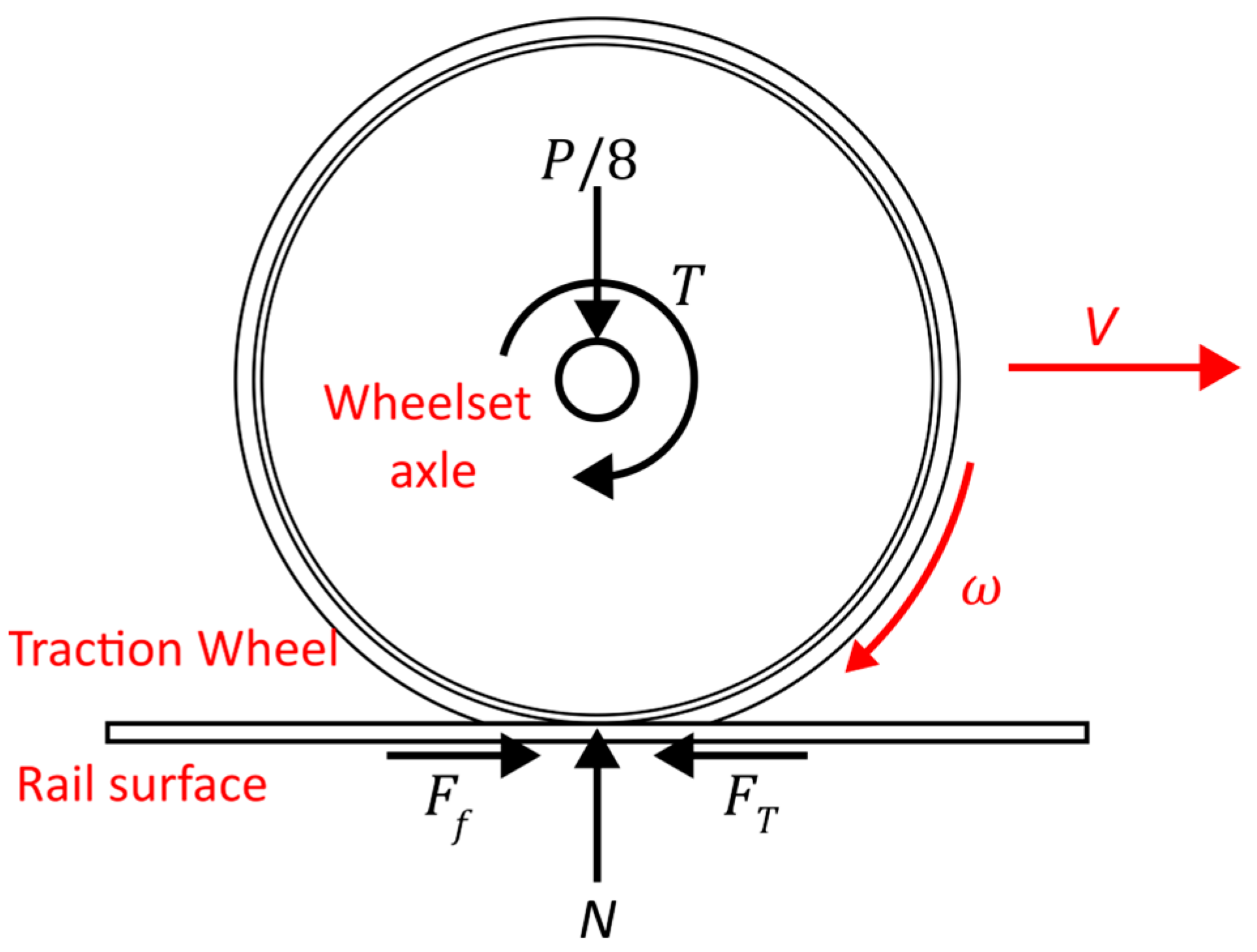
Figure 7.
The process flowchart. The railcar acceleration signals and the wheelset encoder signal are processed to find a correlation.
Figure 7.
The process flowchart. The railcar acceleration signals and the wheelset encoder signal are processed to find a correlation.
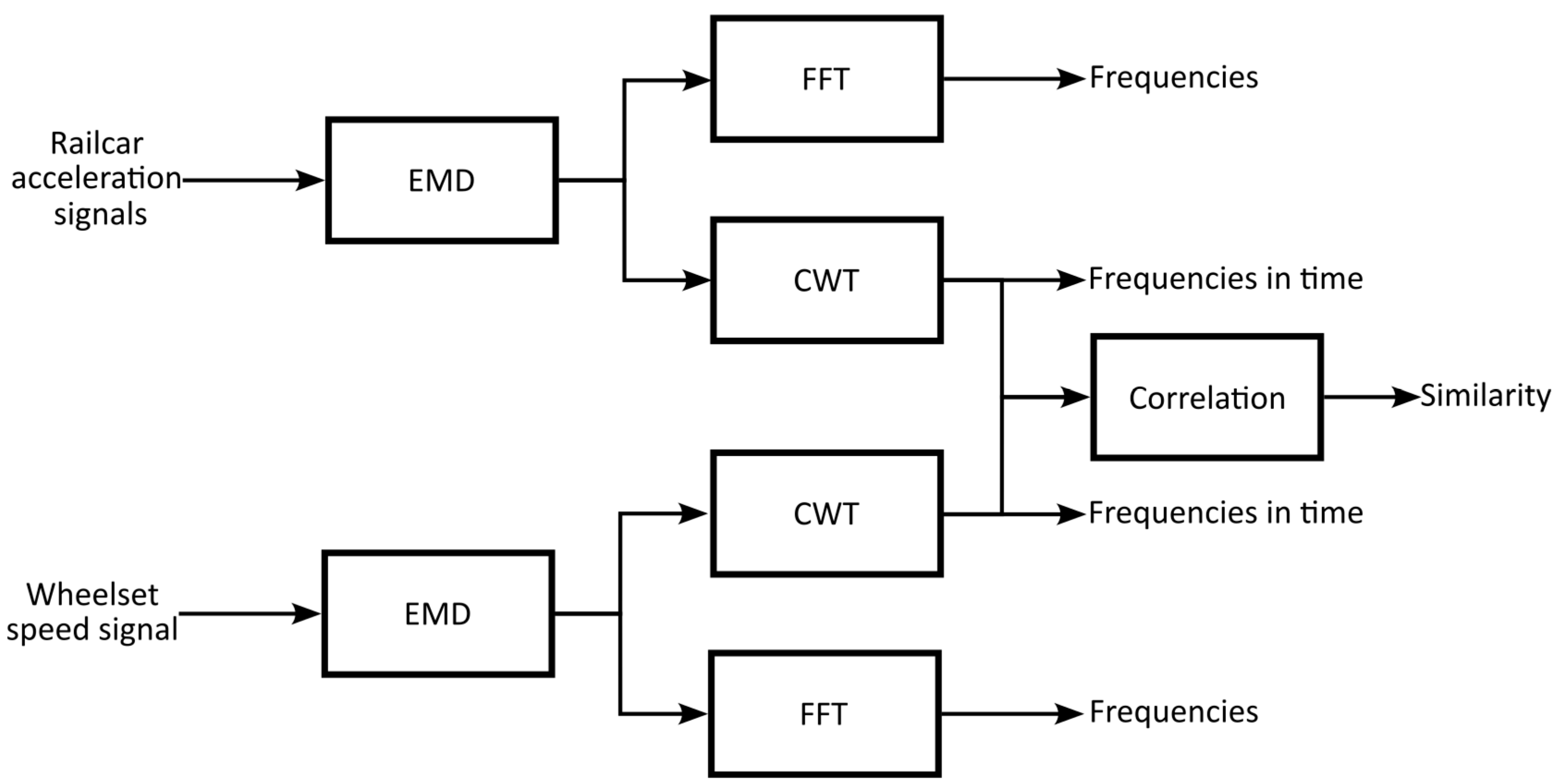
Figure 8.
The proposed correlation algorithm. The procedure described by Equations (2) and (3) is applied to the CWT outputs of each signal. The common frequency components in time reveal the vehicle’s dynamic response due to the tangential forces of the wheel.
Figure 8.
The proposed correlation algorithm. The procedure described by Equations (2) and (3) is applied to the CWT outputs of each signal. The common frequency components in time reveal the vehicle’s dynamic response due to the tangential forces of the wheel.

Figure 9.
Vehicle and wheelset speeds behavior: (a) clean rail test and (b) sand-scattered rail test. The vehicle takes up to 2 s to brake on clean rails, but takes only 0.75 s when the rails are covered in sand.
Figure 9.
Vehicle and wheelset speeds behavior: (a) clean rail test and (b) sand-scattered rail test. The vehicle takes up to 2 s to brake on clean rails, but takes only 0.75 s when the rails are covered in sand.

Figure 10.
The creep curves of the wheel-rail slippage calculated using the data from Figure 9 and Equation (3): (a) clean rails test and (b) sand-scattered rail test.
Figure 10.
The creep curves of the wheel-rail slippage calculated using the data from Figure 9 and Equation (3): (a) clean rails test and (b) sand-scattered rail test.

Figure 11.
CWT and FFT results of the wheelset dynamics 0.4 s prior to braking on clean rails. The CWT results show some frequencies between 120 and 200 Hz, where the most prominent peak is 132 Hz by FFT. The black squares in the FFT spectrum highlight the common frequencies between wheel and vehicle dynamics.
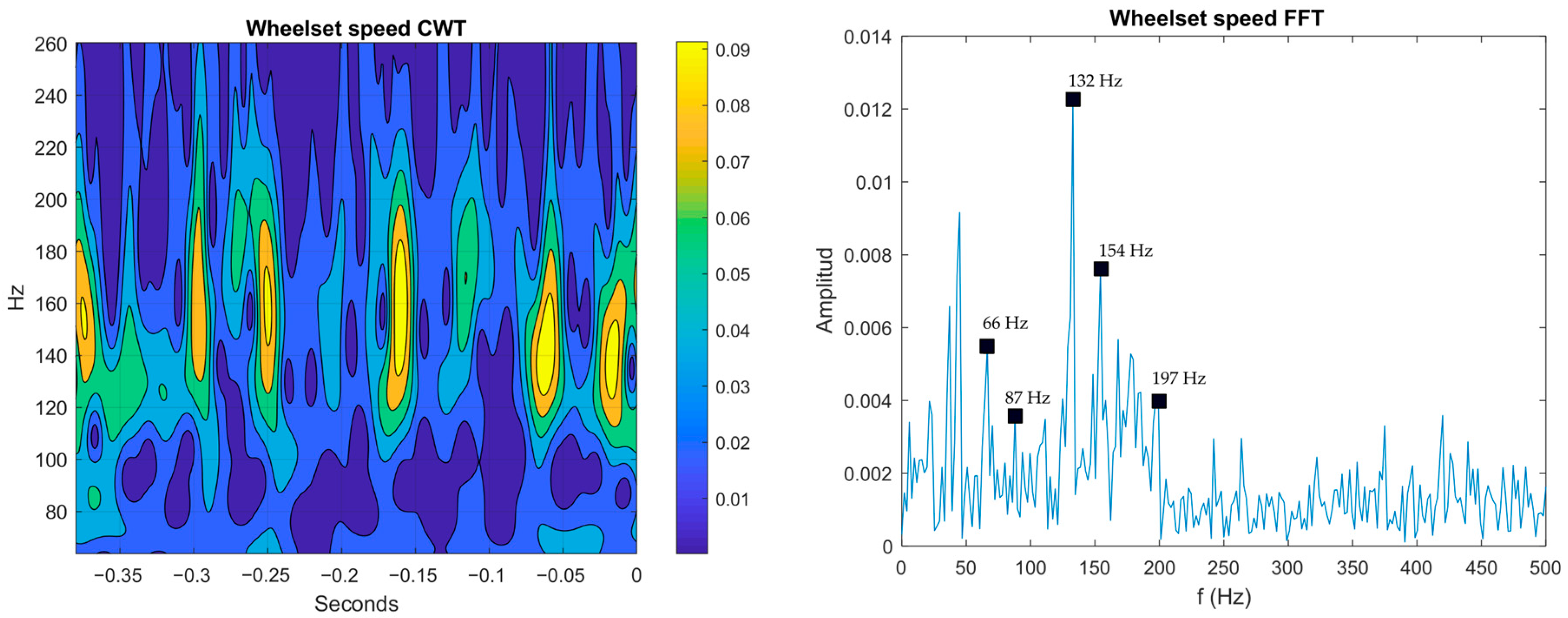
Figure 12.
Frequency analysis results of the vehicle accelerations 0.4 s prior to braking on clean rails in the longitudinal (ax), lateral (ay), and vertical (az) directions. Only lateral and vertical accelerations exhibit a significant correlation between tangential forces and vehicle response.
Figure 12.
Frequency analysis results of the vehicle accelerations 0.4 s prior to braking on clean rails in the longitudinal (ax), lateral (ay), and vertical (az) directions. Only lateral and vertical accelerations exhibit a significant correlation between tangential forces and vehicle response.
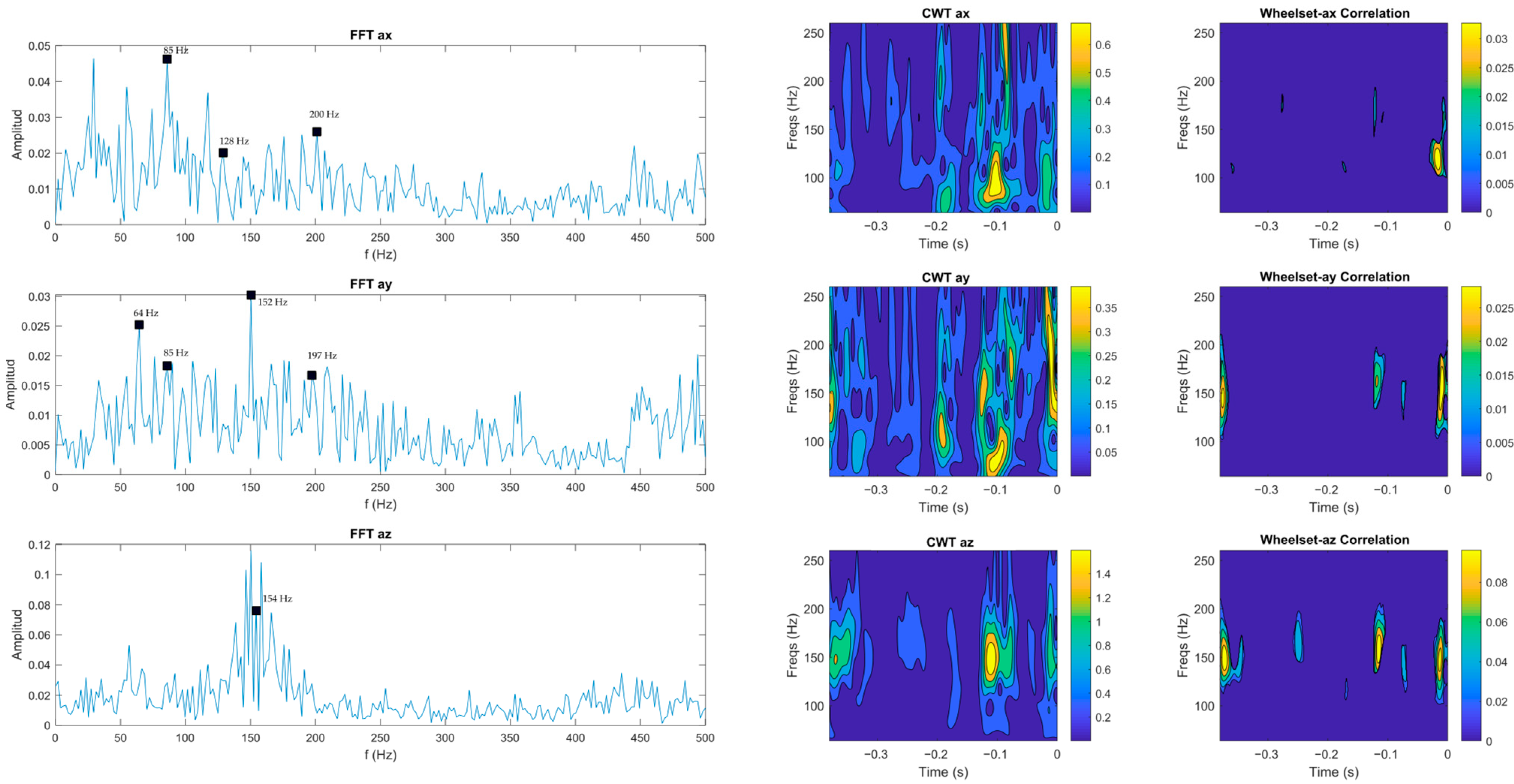
Figure 13.
CWT and FFT results of the wheelset dynamics 0.4 s prior to braking on sand-scattered rails. Both the CWT and the FFT are applied on the same signal within the same time range. The CWT results show many frequencies dispersed all over the spectrogram. The black squares in the FFT spectrum highlight the common frequencies between wheel and vehicle dynamics.

Figure 14.
Frequency analysis results of the vehicle accelerations 0.4 s prior to braking on sand-scattered rails in the longitudinal (ax), lateral (ay), and vertical (az) directions. Many potential matches were found throughout the entire area of the correlation, as a result of brief loads from the wheel. It should be noted that the vehicle vibrates in a regular pattern in the vertical direction.
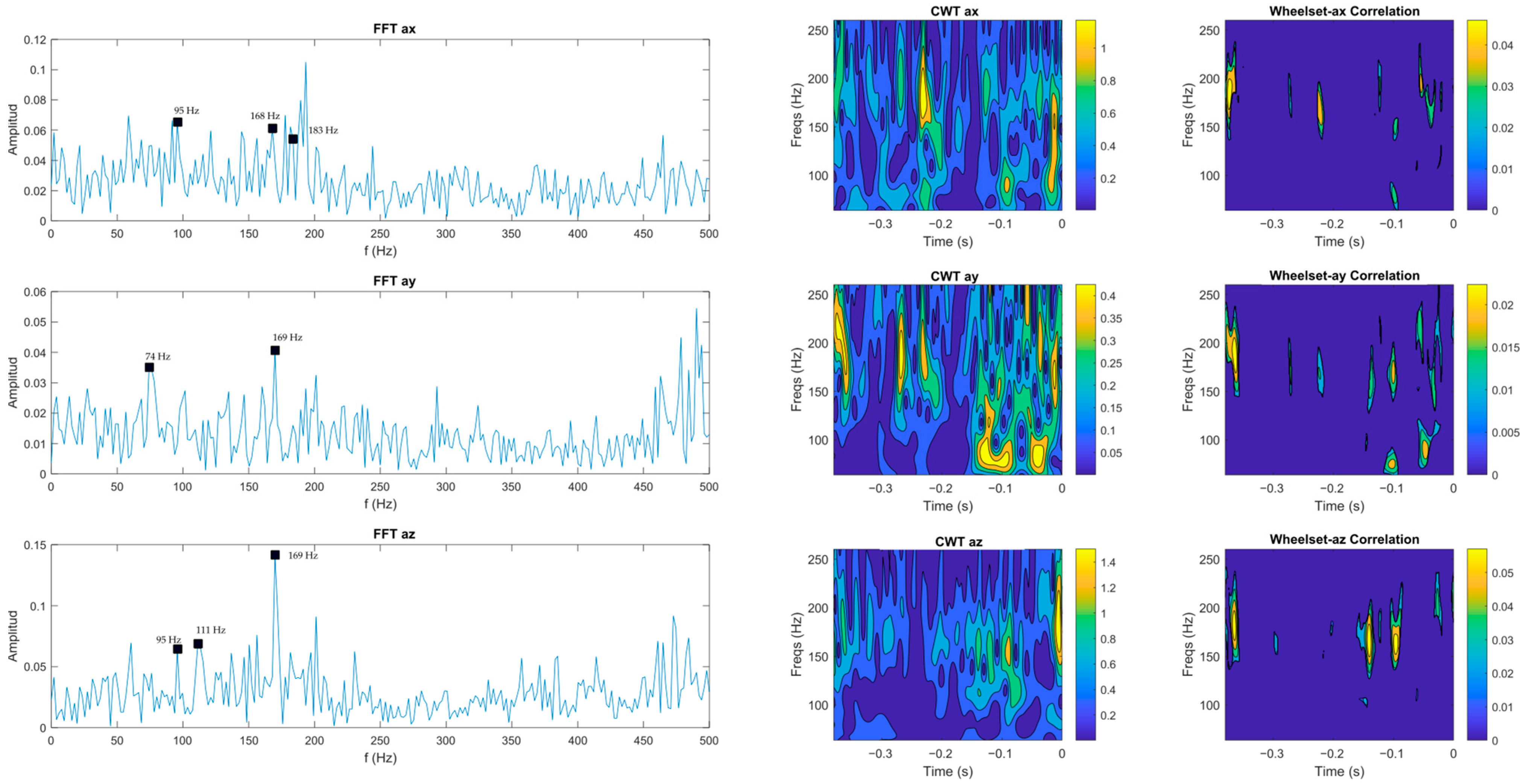
Figure 15.
CWT and FFT results of the wheelset during braking on clean rails. Both the CWT and the FFT are applied to the same signal within the same time range. The CWT results show no regular frequency patterns, principally due to the large creep and low friction coefficient. The black squares in the FFT spectrum highlight the common frequencies between wheel and vehicle dynamics.
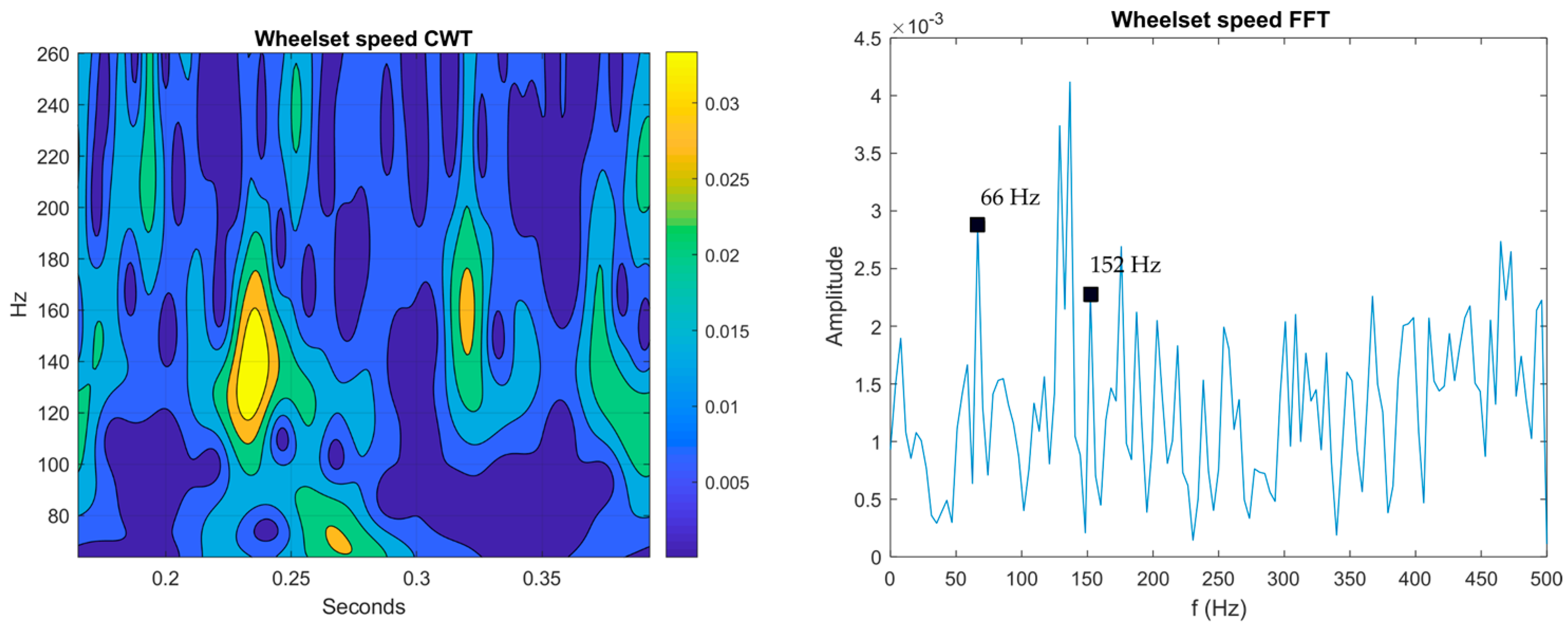
Figure 16.
Frequency analysis results of the vehicle accelerations during braking on clean rails in the longitudinal (ax), lateral (ay), and vertical (az) directions. Because of the low friction coefficient, few tangential forces are transmitted to the vehicle’s body.
Figure 16.
Frequency analysis results of the vehicle accelerations during braking on clean rails in the longitudinal (ax), lateral (ay), and vertical (az) directions. Because of the low friction coefficient, few tangential forces are transmitted to the vehicle’s body.
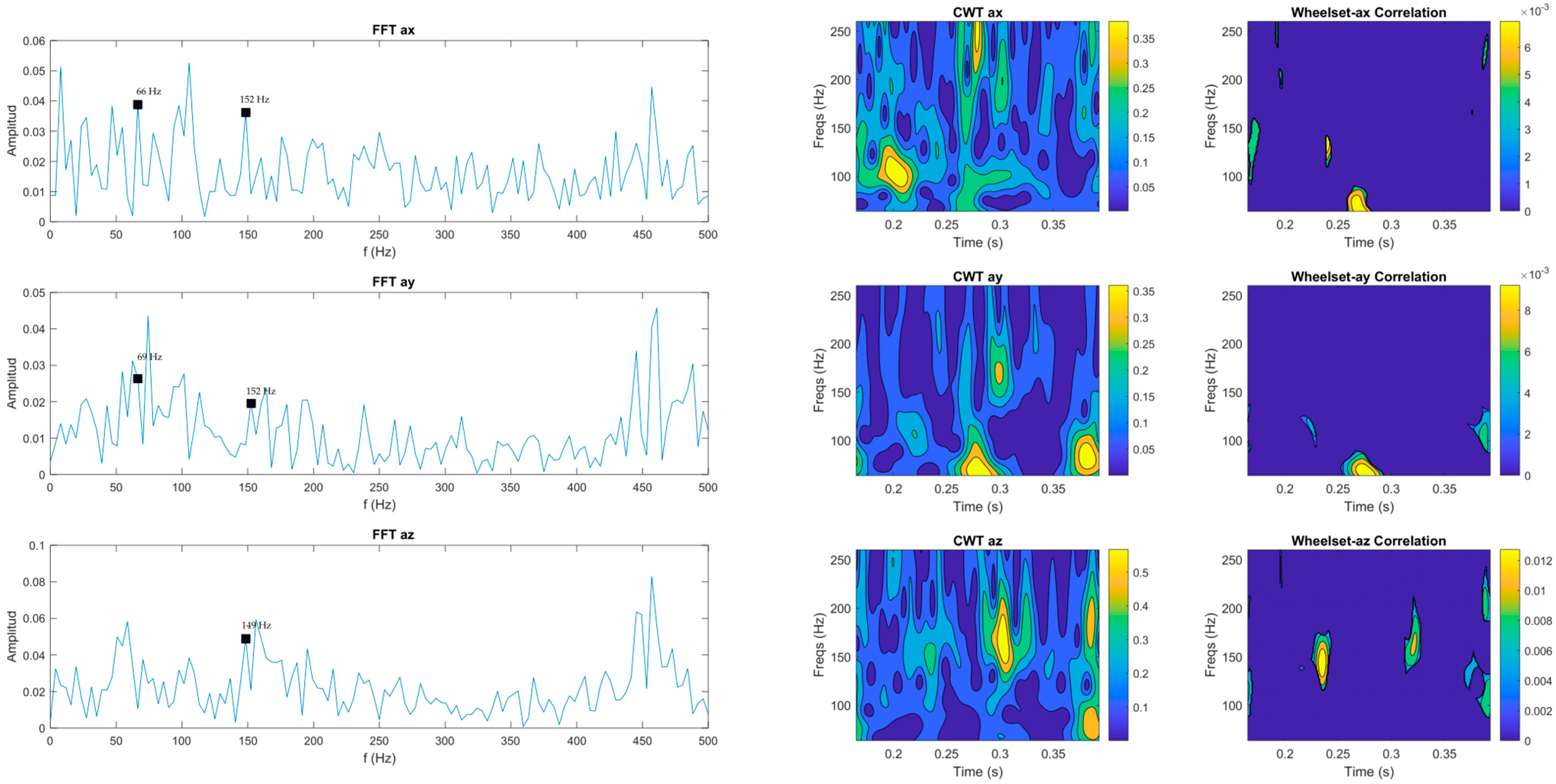
Figure 17.
CWT and FFT results of the wheelset during braking on sand-scattered rails. Both the CWT and the FFT are applied to the same signal within the same time range. The CWT results show a regular pattern in the frequencies probably caused by the intense tangential forces. The black squares in the FFT spectrum highlight the common frequencies between wheel and vehicle dynamics.
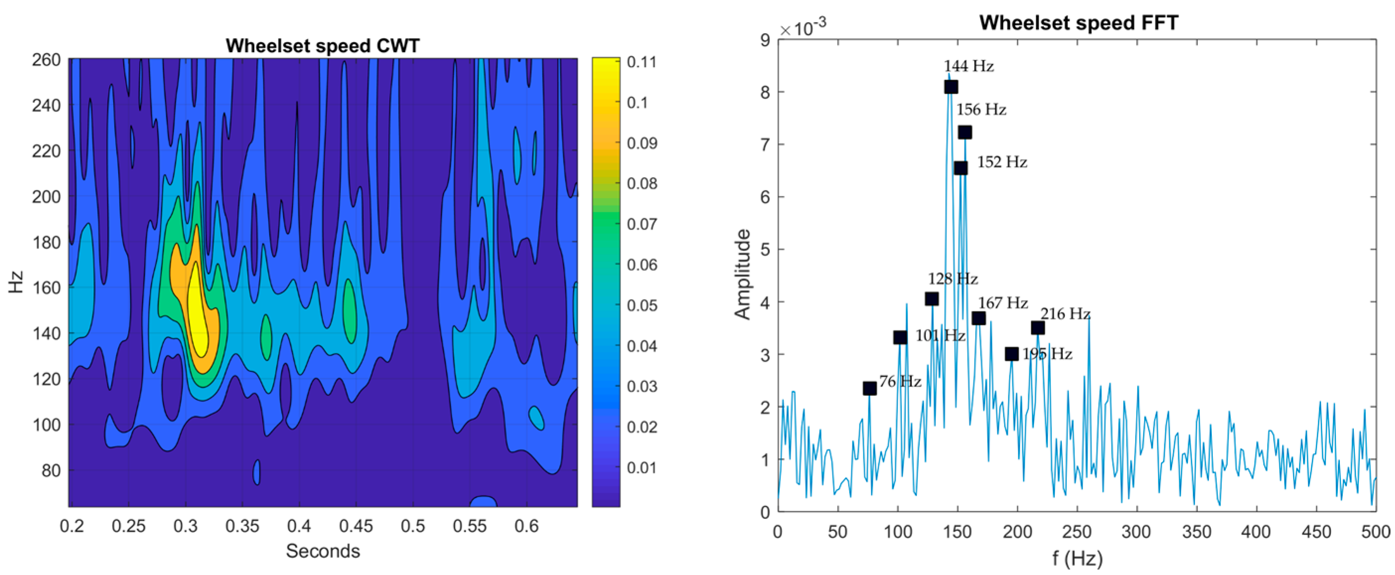
Figure 18.
Frequency analysis results of the vehicle accelerations during braking on sand-scattered rails in the longitudinal (ax), lateral (ay), and vertical (az) directions. The high friction coefficient causes the vehicle to vibrate in all directions. Most of the tangential forces are transferred to the vehicle’s body.

Table 1.
Principal parameters of the railcar.
| Parameter | |
|---|---|
| Mass | |
| 4.4 kg 1.0 kg 0.64 kg 2.76 kg |
| Dimensions | |
| 506 mm 100 mm 120 mm 63 mm 23 mm |
| Suspension stiffness | 5.82 N/mm |
| Center of mass | x: 42 mm y: 0 mm z: 62 mm |
Table 2.
The frequencies of the system.
| Frequency (Hz) | Source |
|---|---|
| 25 | Sleeper passage |
| 46 | Wheel rolling (at vehicle speed 1.2 m/s) |
| 150 | Vehicle vertical |
| 180 | Vehicle lateral |
| 200 | Vehicle longitudinal |
Disclaimer/Publisher’s Note: The statements, opinions and data contained in all publications are solely those of the individual author(s) and contributor(s) and not of MDPI and/or the editor(s). MDPI and/or the editor(s) disclaim responsibility for any injury to people or property resulting from any ideas, methods, instructions or products referred to in the content. |
© 2023 by the authors. Licensee MDPI, Basel, Switzerland. This article is an open access article distributed under the terms and conditions of the Creative Commons Attribution (CC BY) license (https://creativecommons.org/licenses/by/4.0/).
Share and Cite
MDPI and ACS Style
Hurtado-Hurtado, G.; Morales-Velazquez, L.; Otremba, F.; Jáuregui-Correa, J.C. Railcar Dynamic Response during Braking Maneuvers Based on Frequency Analysis. Appl. Sci. 2023, 13, 4132. https://doi.org/10.3390/app13074132
AMA Style
Hurtado-Hurtado G, Morales-Velazquez L, Otremba F, Jáuregui-Correa JC. Railcar Dynamic Response during Braking Maneuvers Based on Frequency Analysis. Applied Sciences. 2023; 13(7):4132. https://doi.org/10.3390/app13074132
Chicago/Turabian StyleHurtado-Hurtado, Gerardo, Luis Morales-Velazquez, Frank Otremba, and Juan C. Jáuregui-Correa. 2023. "Railcar Dynamic Response during Braking Maneuvers Based on Frequency Analysis" Applied Sciences 13, no. 7: 4132. https://doi.org/10.3390/app13074132
Note that from the first issue of 2016, this journal uses article numbers instead of page numbers. See further details here.