
Deep Learning-Based Hip X-ray Image Analysis for Predicting Osteoporosis

1
Department of Orthopedics, National Yang Ming Chiao Tung University Hospital, Yilan 260, Taiwan
2
Department of Computer Science and Information Engineering, National Ilan University, Yilan 260, Taiwan
*
Author to whom correspondence should be addressed.
Appl. Sci. 2024, 14(1), 133; https://doi.org/10.3390/app14010133
Submission received: 29 September 2023
/
Revised: 20 October 2023
/
Accepted: 23 October 2023
/
Published: 22 December 2023
(This article belongs to the Topic Electronic Communications, IOT and Big Data)
Abstract
:Osteoporosis is a common problem in orthopedic medicine, and it has become an important medical issue in orthopedics as Taiwan is gradually becoming an aging society. In the diagnosis of osteoporosis, the bone mineral density (BMD) derived from dual-energy X-ray absorptiometry (DXA) is the main criterion for orthopedic diagnosis of osteoporosis, but due to the high cost of this equipment and the lower penetration rate of the equipment compared to the X-ray images, the problem of osteoporosis has not been effectively solved for many people who suffer from osteoporosis. At present, in clinical diagnosis, doctors are not yet able to accurately interpret X-ray images for osteoporosis manually and must rely on the data obtained from DXA. In recent years, with the continuous development of artificial intelligence, especially in the fields of machine learning and deep learning, significant progress has been made in image recognition. Therefore, it is worthwhile to revisit the question of whether it is possible to use a convolutional neural network model to read a hip X-ray image and then predict the patient’s BMD. In this study, we proposed a hip X-ray image segmentation model and a hip X-ray image recognition classification model. First, we used the U-Net model as a framework to segment the femoral neck, greater trochanter, Ward’s triangle, and the total hip in the hip X-ray images. We then performed image matting and data augmentation. Finally, we constructed a predictive model for osteoporosis using deep learning algorithms. In the segmentation experiments, we used intersection over union (IoU) as the evaluation metric for image segmentation, and both the U-Net model and the U-Net++ model achieved segmentation results greater than or equal to 0.5. In the classification experiments, using the T-score as the classification basis, the total hip using the DenseNet121 model has the highest accuracy of 74%.
1. Introduction
Osteoporosis is one of the most common issues in orthopedic medicine today. People have been facing the challenges of osteoporosis due to the natural process of aging. According to the International Osteoporosis Foundation (IOF), both men and women over the age of 50 have a significant risk of developing osteoporosis, with approximately one-fifth of men and one-third of women falling into this category [1]. The risk of osteoporosis dramatically increases in women after menopause. It is estimated that there are approximately 200 million women worldwide who are affected by osteoporosis. As our country is gradually transitioning into an aging society, the percentage of people afflicted by osteoporosis is steadily on the rise. Consequently, effective prevention and treatment of osteoporosis have become vital concerns in the field of orthopedic medicine [2]. In the early stages of osteoporosis, there are no obvious symptoms, but fractures may occur because of minor injuries [3]. In severe cases, fractures may occur not only in the hip but also in the spine, wrist, arm, and knee. Ultrasound [4], peripheral bone densitometry, etc., are the main instruments used by orthopedic surgeons to diagnose osteoporosis. However, the image of the hip formed by these methods is more difficult for the orthopedic surgeon to read with his/her own eyes and requires the use of more sophisticated instruments, such as dual-energy X-ray absorptiometry (DXA) [5]. The bone mineral density (BMD) of the hip is calculated and compared to the T-score of a younger, healthier person to diagnose osteoporosis [6]. Currently, in the clinical diagnosis of the orthopedic hip, physicians base their diagnosis of osteoporosis on a DXA report of the femoral neck in the hip and the total hip. BMD from DXA is the main criterion for diagnosing osteoporosis. In Taiwan, because DXA is expensive and limited in number, the popularity of the equipment is far less than that of X-ray imaging, and only high-grade hospitals or nursing homes are equipped with this equipment, while in some remote areas or villages, it is not convenient to use this resource. In some remote areas or rural areas, it is not convenient to use this resource, and cheaper equipment such as ultrasound and peripheral densitometry is mostly used for diagnosis, resulting in a less accurate and less efficient diagnosis of symptoms.
Currently, physicians are unable to manually read X-ray images for osteoporosis in clinical diagnosis. Early diagnosis of osteoporosis is important for the prevention of osteoporotic fractures, and in recent years, artificial intelligence has been gradually introduced into medical diagnosis [7]. As machine learning and deep learning methods have made significant advances in image recognition, it is worthwhile to revisit the question of whether or not it is possible to use convolutional neural networks (CNNs) to read a hip X-ray image and further predict a patient’s BMD status, and the answer may be affirmative. While traditional machine learning methods can be effective, they rely on manual feature extraction, sequential training of the model, and output of the results. With the great leap in hardware computing power of graphics processing units (GPUs), deep learning can directly input data into the model, and the neural networks will extract the features by themselves when they train the model and then output the results. Compared with machine learning, deep learning omits the part about manual feature extraction. When the amount of data is relatively large, deep learning can extract more features, and the output results will be better than traditional machine learning.
In this study, we collected data from 134 orthopedic patients, most of whom were menopausal women and elderly men. The data collected were patients’ left or right hip X-ray images and DXA diagnostic data, of which the DXA diagnostic reports were femoral neck, greater trochanter, Ward’s triangle, and total hip BMD and T-score. We used image segmentation, image matting, data augmentation, and DXA reports to classify the BMD and T-score values of the hip X-ray images and designed the experiments using a deep learning algorithm model to predict the BMD and T-score of the hip. A deep learning algorithm model was used to design an experiment to predict whether the femoral neck, greater trochanter, Ward’s triangle, and overall hip findings on hip X-ray images constitute osteoporosis and to establish a risk classification model of osteoporosis to assist orthopedic surgeons in diagnosis, hoping to reduce the surgeon’s time spent in diagnosis.
The research question of this study is divided into two parts. The first part is that in image segmentation, the segmentation results of four areas (femoral neck, greater trochanter, Ward’s triangle, and total hip) on X-ray images may affect the subsequent image classification results and whether the segmentation model can correctly and efficiently segment the contours of the four areas for subsequent image classification experiments to be conducted. The second part is in the depth learning method: what are the prediction results of different models, and which model builds the best prediction of osteoporosis and can more accurately predict the BMD of patients? In addition to exploring the correlation between the interpretation of hip X-ray images and BMD and the experimental accuracy of the depth model, we also analyzed two more areas of the hip, namely the greater trochanter and the Ward’s triangle, to provide physicians with more aspects to diagnose and analyze the patients. The study will be carried out using CNN and supervised learning methods. This study will also use CNNs and supervise learning to mark the femoral neck, greater trochanter, Ward’s triangle, and whole hip as the data input of the whole experiment, and then the results of the experiment will be further explored, hoping to provide some help for the medical diagnosis of osteoporosis.
2. Related Works
2.1. Osteoporosis
Osteoporosis is a silent disease that may not cause pain before fractures occur, but as a person ages, their bone mass continually decreases in the body. Osteoporosis reduces the body’s bone mineral density (BMD) and causes fragility of the bones in the hip, spine, and wrist. It also leads to fractures and other complications (e.g., intervertebral compression fracture, hip and wrist joint fracture, etc.), which is a disease of bone metabolism [8]. Bone is a self-renewing, active tissue. In the process of maintaining bone health, the body continuously breaks down old bone and replaces it with new bone tissue. During childhood and adolescence, new bone formation occurs rapidly, resulting in larger BMD values, which reach their peak around the age of 20. In the following 7 to 10 years, the rate of new bone production is about the same as the rate of decomposition of old bone, and the adult skeleton reaches complete renewal [9]. However, when people reach about 40 years old, the rate of bone mineral increase slows down. At this point, the rate of decomposition of bone is greater than the rate of new bone production, and the shell of the bone becomes thinner, making it more fragile.
In bone density examination, DXA calculates BMD as a direct reference indicator, and the lower the value of BMD, the more likely you are to get osteoporosis. Another commonly used indicator is the T-score, which is regarded as an extension of the BMD calculation as a basis for assessing the presence or absence of osteoporosis. The T-score is calculated by dividing the difference between the BMD calculated by a specialized instrument such as DXA and the expected young normal (YN) by the standard deviation (SD) of the BMD in young people [10]. The T-score’s formula is defined as the following Equation (1):
T-Score = (BMD − YN)/SD
According to the standard definition of the World Health Organization [11], a T-score greater than −1 indicates normal bone mass, less than or equal to −1 or greater than −2.5 indicates low bone mass, and less than or equal to −2.5 indicates osteoporosis. As humans age, bone loss is inevitable, so when the age gradually increases, the two numerical indicators of bone density and T-score will be lower than those of young people. In the clinical diagnosis of osteoporosis in the hip, the diagnosis of osteoporosis is based on a DXA report of the femoral neck and the total hip.
2.2. Machine Learning and Deep Learning in Orthopedics
2.2.1. Osteoporosis Detection
In recent years, the rise of artificial intelligence has become more common in the medical industry, with machine learning and deep learning as the main applications. In 2016, a study was proposed by S.K. Hong et al. that primarily utilized machine learning and deep learning to assist orthopedic surgeons in determining the presence of osteoporosis. The study involved collecting DXA diagnosis results from men aged 50 and above as well as postmenopausal women. The focus of the study was on the femoral neck in hip X-ray images. Unlike our study, which solely utilized hip X-ray images as the dataset, their study incorporated various covariates (e.g., height, age, etc.) as part of the dataset. Under this prerequisite, it is easier to predict better results. They employed an artificial neural network (ANN) to perform binary classification of osteoporosis based on T-scores. The results were promising when evaluating men aged 50 and above and postmenopausal women. In this study, the accuracy for men reached 85.8%, with a sensitivity of 81.6% and a specificity of 90.0%. For women, the accuracy was 86.2%, with a sensitivity of 84.7% and a specificity of 87.7% [12]. In addition, Support Vector Machine (SVM) outperforms Logistic Regression (LR) in predicting osteoporosis risk and surpassed some traditional clinical decision tools, such as the Osteoporosis Self-Assessment Tool (OST), Osteoporosis Risk Assessment Instrument (ORAI), Simple Calculated Osteoporosis Risk Estimation (SCORE), and Osteoporosis Index of Risk (OSIRIS). In 2013, T.K. Yoo et al. achieved a predictive accuracy of 77%, sensitivity of 78%, and specificity of 76% by collecting medical records of postmenopausal women [13].
In addition to DXA, in 2021, J.W. Adams et al. proposed the application of neural networks for screening application analysis in osteoporosis [14], which utilizes low-frequency radiofrequency data passing through the wrist and uses a multilayer perceptron (MLP) to do the analysis, and in 2020, B. Zhang et al. proposed to train a CNN model based on lumbar spine X-ray images to read osteoporosis and bone loss [15], which are also of great help for orthopedic applications. In 2020, N. Yamamoto et al. used ResNet, GoogLeNet, and EfficientNet to classify hip X-ray images for osteoporosis [16]. They employed a T-score for binary classification and focused solely on hip X-ray images, achieving the highest accuracy of 84% in the experiments conducted with GoogLeNet and EfficientNet B3. The difference from our study is that in their dataset of 1131 hip X-ray images, 708 were from patients with confirmed hip fractures. Patients with hip fractures typically have lower bone density, which is a key indicator of osteoporosis. Therefore, the ability to distinguish between those with and without osteoporosis was more pronounced in cases of confirmed hip fractures. The difficulty is how to predict the correct bone density in normal hip X-ray images. In the same study of determining whether hip X-ray images are osteoporosis, the experimental model proposed by R. Jang et al. in 2021 was dichotomized by T-score, and the experimental model mainly uses a deep neural network (DNN) developed based on VGG16 architecture, with an optimal accuracy of 81%, sensitivity of 91%, and specificity of 69% [17]. However, in this past study, only hip X-ray imaging data were included in postmenopausal women clinically at high risk for osteoporotic fractures. Furthermore, the data set is limited to women. It does not cover male hip X-rays, where bone density is more difficult to predict.
2.2.2. Fracture Detection
Often, with osteoporosis at the same time, there are compression fractures, and patients with severe osteoporosis do not need much movement to cause a spinal compression bone fracture. The same as osteoporosis, spinal compression fractures can also use deep learning to make predictions. In 2018, F. Cabitza et al. proposed a literature review of spinal bone image segmentation and osteoarthritis fracture prediction [18], focusing on the literature on the application of machine learning and deep learning methods in medicine and biology in the past ten years, among which the most widely used in medical imaging are machine learning SVM and deep learning. The use of deep learning has been increasing year by year, and it has become the bulk trend. The proportion of evaluation indexes used in the model is also summarized, and the results show that the accuracy rate accounts for 45% of the indexes that most experiments will evaluate, and the sensitivity and specificity of the model evaluation indexes account for 25%, which is more common in medical and biological research.
In 2020, W. Abbas et al. used Faster R-CNN to detect and classify fractures in lower leg X-rays [19], collecting X-ray images of lower leg fractures from 50 patients. The Faster R-CNN model achieved 94% accuracy, sensitivity, and specificity of 96% and 90%, respectively. In addition, Y. Yamada et al.’s study used deep learning to determine whether a hip fracture was a fracture based on X-ray images of the anteroposterior and lateral hip positions [20], and the accuracy of hip fracture classification was 98% after model training, which was better than the 95% of the orthopedic surgeon’s interpretation. In addition to the spine and hip, J. Olczak et al. used machine learning to make predictions on X-rays of the wrist and ankle [21], and VGG16 had a good effect in determining fracture with an accuracy of 83%. S.W. Chung et al. labeled normal shoulder X-ray images and four abnormal proximal humerus fracture types and then used image enhancement and CNN model training to predict whether a fracture occurred [22]. The accuracy of determining a normal shoulder and proximal humerus fracture was 96%, the sensitivity was 99%, and the specificity was 97%, which was higher than the accuracy of an orthopedic surgeon’s diagnosis.
2.3. Image Segmentation
In medical imaging, both high- and low-level features of medical images are very important, but the traditional image segmentation method takes more time to filter out the unnecessary noise of medical images. Therefore, this study uses U-Net with simple image semantics and an advanced extended U-Net++ architecture to produce a good effect on the medical images through feature splicing, so that overfitting is not easy to form. U-Net model architecture was proposed by O. Ronneberger et al. in 2015 [23]. The left half of the U-Net model architecture is the Encoder, which is part of feature extraction. It consists of a series of subsampling modules composed of convolution layers (ReLU) with 3 × 3 kernels and 2 × 2 max-pooling layers, which reduce dimensionality and increase the number of channels. Subsampling performs image information restoration, and upsampling performs image pixel recovery, and then the extracted features are passed down the line. The right half of the model structure is the Decoder, which is part of upsampling. Upsampling has a 2 × 2 convolution kernel and Skip Connection for feature fusion, and finally, a 1 × 1 convolution layer is used to output the result. The model architecture of U-Net++ was proposed by Z. Zhou et al. in 2018 [24]. The difference between U-Net++ and U-Net architecture is that the jump connection is mainly redesigned in U-Net++, which is used to fill the semantic difference between Encoder and Decoder feature mapping, improve feature fusion in Decoder, and make semantic feature mapping easier to optimize. In addition, dense jump connection paths are added to improve the performance of image segmentation. The U-Net++ architecture also adds more depth supervisors to prune the model to adjust the model complexity and changes some loss functions, combining cross entropy and dice coefficient, to increase the performance of the model.
2.4. Deep Learning Neural Network Models
2.4.1. Convolutional Neural Networks (CNNs)
In 2012, A. Krizhevsky et al. proposed the classical CNN model [25]. CNN is the process of obtaining various useful convolution kernels through the neural network learning method of backpropagation, which is mainly divided into three parts: (1) the convolution layer, (2) the pooling layer, and (3) the fully connected layer. The CNN model has an additional convolution layer and a pooling layer compared to traditional deep learning networks. The convolution layer and the pooling layer are for feature extraction, while the fully connected layer is for classification. The convolution layer is used to reduce the dimensionality of the image and convolves the image with a feature detector. The pooling layer is used to replace a certain area of the image with a value to reduce the size of the image, block the feature image to reduce the feature map dimension, retain important features, and obtain the pooled image, which also includes avoiding overfitting. There are three main approaches: max pooling, mean pooling, and stochastic pooling. The most common is max pooling. Each neuron in the full connection layer is connected to the neuron in the upper layer, and each connection has a different weight value. The full connection layer will integrate all the useful information from the previous results and then flatten the neural network. Flatten to the neural network, which is responsible for producing the final classification result in the softmax activation function.
2.4.2. VGGNet
VGGNet was published in 2014 by K. Simonyan et al. from the Visual Geometry Group of the University of Oxford [26]. Its architecture is simple; the number of weights is very large, and it contains convolutional kernel weights and fully connected layer weights. The number of channels from VGGNet is large, and the number of channels in the first layer is 64. Each layer will be doubled later; the maximum number of channels reaches 512; the number of channels increases, which means that more information can be extracted; and many convolution kernels are used. The size is 3 × 3. VGGNet contributes to deepening the model by using smaller stacks of convolutional kernels, and by deepening the network of the model, it can be improved in terms of the ability of the model to be simulated. VGGNet has the advantage of a simpler structure. All networks use the same size of convolutional kernel (3 × 3) and the largest pooling layer (2 × 2). The disadvantage is that VGGNet has many parameters, which take up a large amount of memory space. The common ones are VGG16 and VGG19. The VGG16 model used in this study consists of 13 convolutional layers, three fully connected layers, five pool layers, and softmax output layers.
2.4.3. ResNet
In 2015, ResNet [27] was proposed by K. He et al. Greatly solved the vanishing gradient problem of deep networks, and it was pointed out in the paper that the result of a 20-layer network would not be worse than that of a 56-layer network, and there would be a degradation problem as the network layer gets deeper. The introduction of residual learning (RL) can maintain accuracy and speed even when the network layer is deepened, while the softmax layer is composed of the gradient-log-normalizer (GLN) function, which contains the classification rate distribution. The architecture of ResNet can adjust the depth and width of the model by adjusting the number of channels in the block and the stacking of the blocks, which makes the model easier to optimize, and its invention has solved the degradation problem of deep neural networks. The common ones are ResNet50, ResNet101, and ResNet152. ResNet50 is used in this study.
2.4.4. DenseNet
The architecture of DenseNet was proposed by G. Huang et al. in 2018 [28], and gradients disappear as the network gets deeper. The basic idea is the same as ResNet: DenseNet does not use a very deep or wide network to obtain image recognition effects, but by increasing the fluidity of features and reducing the complexity of the network, the gradient can be obtained from the loss function in each layer of the network, which solves the problem of gradient disappearance. Compared with ResNet’s splicing of feature maps, DenseNet has the role of summation, connecting the front network layer with the following network layer and reusing network features. DenseNet is a more simplified model with a lower parameter calculation cost than ResNet. Common ones are DenseNet121, DenseNet169, and DenseNet201. DenseNet121 was used in this study.
3. Research Methods
3.1. Research Framework
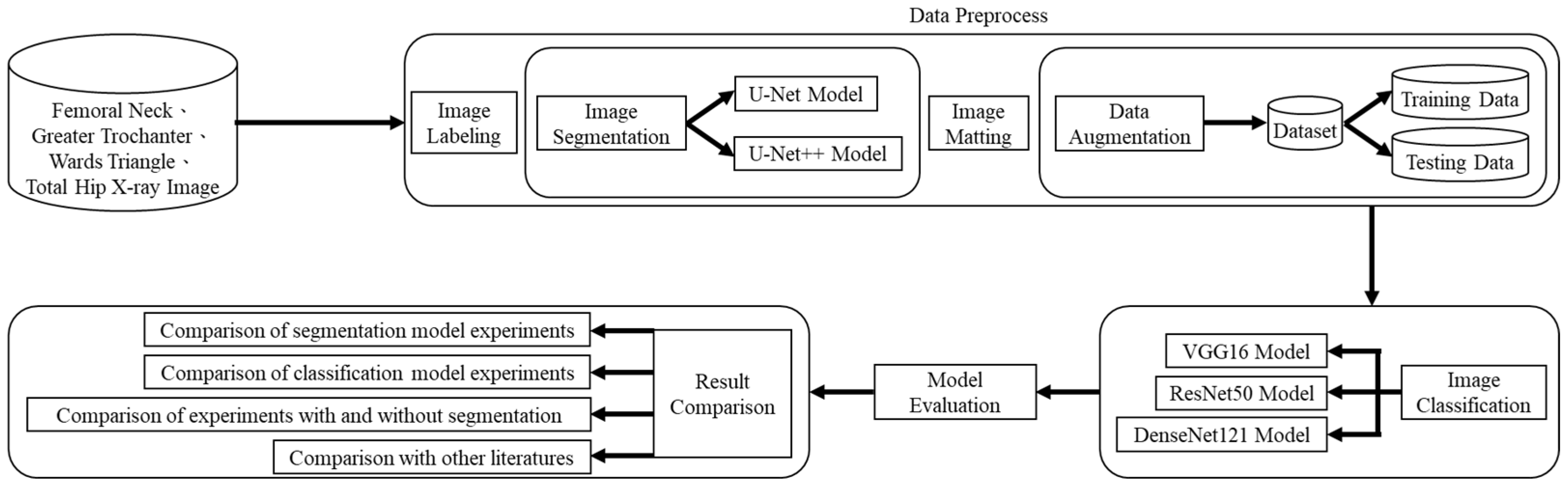
The research framework and process of this study are shown in Figure 1, which is divided into four parts: (1) dataset, (2) data preprocessing, (3) image categorization, and (4) result comparison. After obtaining the dataset from the hospital, data preprocessing (including image labeling, image segmentation, image matting, and data augmentation) was performed, and then three different convolutional neural network models were used to categorize the X-ray images of the four parts of the hip, and the classified X-ray images of the hip were divided into three different datasets for the test. The first one is the original X-ray images to verify whether the model training with the original dataset will result in underfitting and poor generalization due to the low complexity of the model and the small number of features in the images. The second type is the X-ray image after data augmentation, which aims to verify whether the data augmentation can effectively improve the overall results and enhance the generalization ability of the model. The third is based on the results of the classification experiments with the best performance in the T-score and BMD classifications of the first two types of data and adding the image segmentation method to verify whether the overall results can be improved. Finally, the results of the segmentation model experiment, the classification model experiment with or without data augmentation, and the classification model experiment with or without image segmentation were compared.
3.2. Datasets
The source of X-ray images for this study were patients in a regional hospital in Taiwan from September 2020 to September 2021, a period of A total of 134 left or right hip radiographs and DXA diagnoses were collected from 134 patients, mostly elderly men and postmenopausal women, in a retrospective study to collect a dataset that was reviewed by the Institutional Review Board for Research Ethics Programs and Studies (IRB). A total of 139 left and right hip radiographs were collected, and for the DXA images, each DXA image had a diagnostic interval distribution of BMD and T-score values for the femoral neck, greater trochanter, Ward’s triangle, and total hip, but because the DXA models were divided into two types, one model only displays bone density and T-score data for the femoral neck and total hip and lacks data for the greater trochanter and Ward’s triangle. Further screening of the DXA reports showed 139 data for the femoral neck and total hip and 72 data for the greater trochanter and Ward’s triangle, with an 8:2 ratio of training set to test set data for each part, resulting in 111 training data for the femoral neck and total hip and 57 training data for the greater trochanter and Ward’s triangle. In this study, before the image segmentation experiment, the collected X-ray images were used to mark the contour for each of the four parts for subsequent image segmentation experiments.
3.3. Data Preprocess
3.3.1. Image Labeling
In this study, X-ray images of each of the four areas of the patient’s hip (femoral neck, greater trochanter, Ward’s triangle, and total hip) were separated and manually labeled using Labelme, an open-source tool that can be used for labeling [29]. The four parts of the hip were then framed as shown in Figure 2 below, and the labeled image data were batch converted into binary png files, which were used as inputs for the supervised learning training of U-Net, U-Net++, and image categorization in the image segmentation process.
3.3.2. Image Segmentation
In this study, four parts of the image labeled X-ray images were used in image segmentation by feeding them into U-Net and U-Net++ models for training, and the bit depth of the four parts of the image was converted from the original 24 bits to 8 bits before the model training. The reason for choosing to use U-Net and U-Net++ is that their model structure is simpler, they do not need to spend a lot of time filtering out the remaining noise in the medical images, and they are less likely to form overfits for a small number of image datasets. The binary segmentation prediction results obtained after training the models of U-Net and U-Net++ are shown in Figure 3 below.
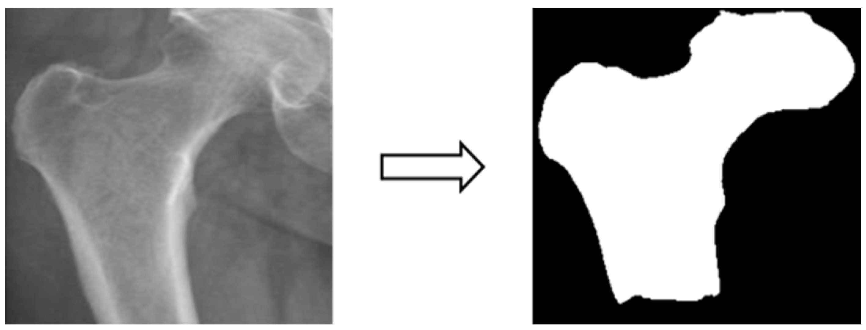
3.3.3. Image Matting
Based on the four parts of the image segmentation of the binary image and the original X-ray image together, the original X-ray image only retains the part of the image segmentation as shown in Figure 4; the other non-part of the contour of the background is removed, and the image is de-behind in the hope that it can enhance the accuracy of the classification of the depth of the learning process, and then the image classification will be segmented images and not segmented images will be compared.
3.3.4. Data Augmentation
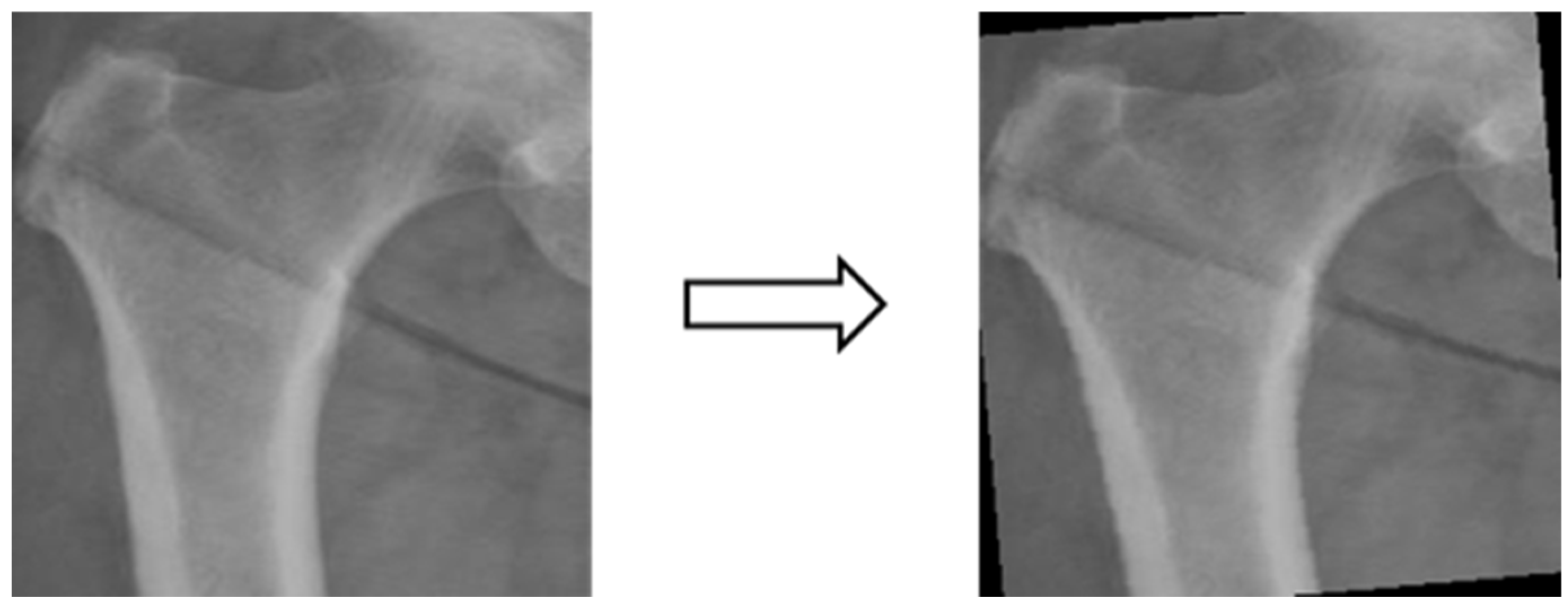
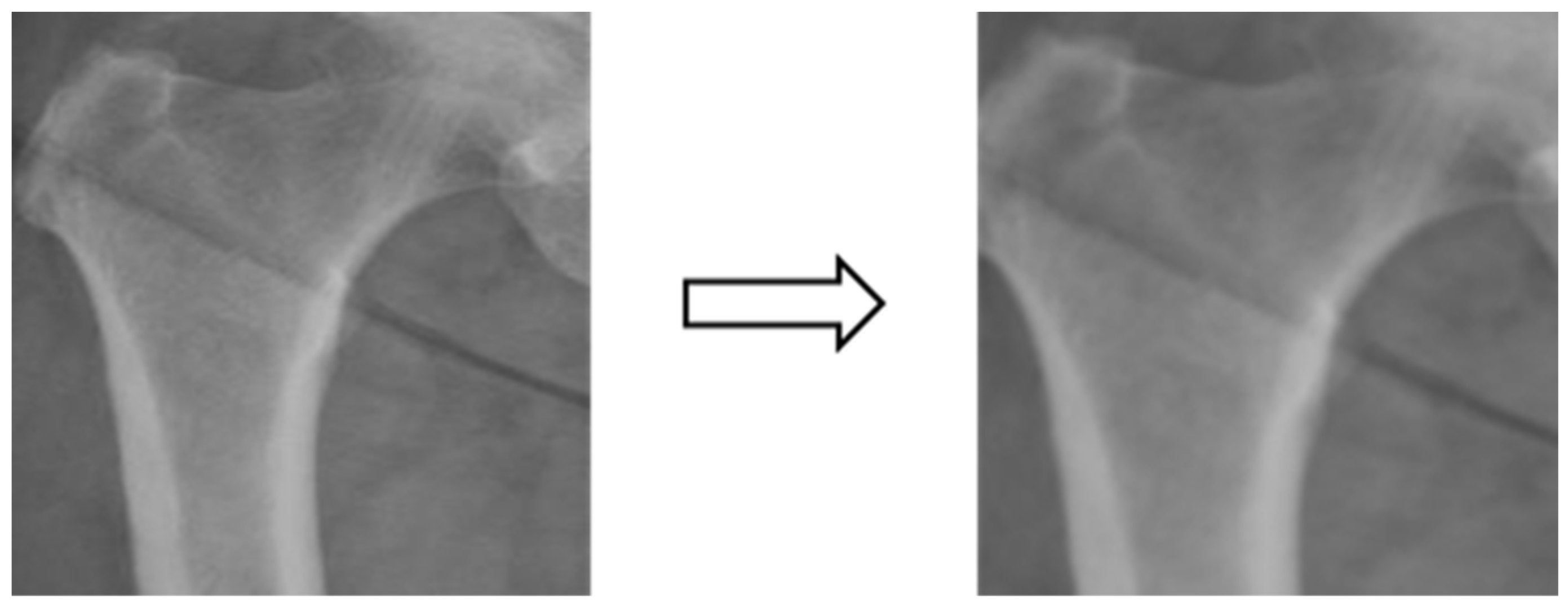
In this study, the X-ray image data were insufficient for image classification experiments. Training the model with the original dataset could lead to issues such as model underfitting and poor generalization due to the low complexity of the model and the limited image features. Therefore, the dataset consisting of X-ray images from four different body areas was augmented by applying transformations like rotation (e.g., Figure 5), shifting (e.g., Figure 6), and random scaling (e.g., Figure 7). Importantly, these augmentations were performed without altering the bone contour morphology, background, or color. The purpose of data augmentation was to aid in the training of deep learning models [30]. Additionally, data augmentation serves to address underfitting problems in classification experiments and can potentially enhance experimental accuracy if overfitting issues arise in the future [31]. Table 1 presents a comparison of data volume before and after data augmentation.
After data expansion through rotation and shifting, each part is expanded by seven times the amount of data, and after expansion, a random scaling method is added so that each batch of data is randomly scaled by between −20% and 20% to achieve the effect of increasing data plurality.
3.4. Experimental Design
3.4.1. Model Evaluation Indicators
Using Intersection over Union (IoU) in object detection for image segmentation [32]. The IoU is calculated by dividing the intersection of two object images by the union, and when the experimental result is greater than or equal to 0.5, it will be regarded as a valid image segmentation result, and the IoU is calculated as the following Equation (2):
IoU = (Area of Overlap)/(Area of Union)
In the part of deep learning image classification, the common evaluation method is accuracy, but in medical and biological research, if we only rely on accuracy, the model evaluation may not be complete enough. Plus, other evaluation methods can make the model evaluation more complete. Before explaining the evaluation indexes of the other models, we will first define the confusion matrix of True Positive (TP), False Positive (FP), False Negative (FN), and True Negative (TN) to facilitate the calculation, as shown in Table 2 below.
This study belongs to medical image classification, and there are four model evaluation indexes derived using a confusion matrix, which are accuracy, sensitivity, specificity, and F1-score. Each of the model evaluation indexes is defined in Table 3, and the relevant formulas are as follows in Equations (3)–(6):
Accuracy = (TP + TN)/(TP + FP + FN + TN)
Sensitivity = TP/(TP + FN)
Specificity = TN/(TN + FP)
F1-score = 2TP/(2TP + FP + FN)
3.4.2. Osteoporosis Classification Index
There are two common diagnostic indexes for the diagnosis of osteoporosis: one is the BMD calculated by DXA, and the other is the T-score, which is regarded as an extension of the calculation of BMD. The T-score serves as a more representative criterion for osteoporosis diagnosis. Therefore, we used these two indexes as the classification indexes for the subsequent in-depth learning experiments. Bone density was categorized into normal bone mineral and abnormal bone mineral according to the DXA diagnostic images corresponding to the patient’s age, and T-score was categorized into not suffering from osteoporosis (T-score > −2.5) and suffering from osteoporosis (T-score ≤ −2.5) according to the DXA diagnostic images, as shown in Table 4 below.
3.4.3. Deep Learning Model Training
In this study, the model training was divided into two parts: image segmentation and image classification. Image segmentation was performed using radiographic images of the femoral neck, greater trochanter, Ward’s triangle, and total hip. The labeled images of the four areas were input into the U-Net and U-Net++ models for training, and the results of the two model experiments were compared after binary segmentation of the images was generated by U-Net and U-Net++. Regarding the U-Net and U-Net++ models, we utilized the Adam optimizer, cross entropy loss function, batch size set to 2, and learning rate = 0.00001. For image classification, the X-ray images of the four parts of the body were divided into two categories according to the above-mentioned bone density and T-score indexes, and the experiments were conducted to compare the segmented and non-segmented images, and then VGG16, ResNet50, and DenseNet121, which are the innovative pre-trained models of deep learning, were used for the image classification experiments in this study after fine-tuning the models. Mreover, VGG16, ResNet50, and DenseNet121, which are innovative deep learning pre-trained models in recent years, were fine-tuned to be used as the image classification experiments in this study. In this study, we used the Adam optimizer, cross-entropy loss function, batch size set to 16, and a lower learning rate of 0.000001 in the image classification experiments. All these parameter settings were determined as the optimal parameters through multiple rounds of testing. Additionally, we added a dropout layer and a dense layer to the model structure. The purpose of the dropout layer is to avoid the over-simulation problem in the subsequent experiments, and the dense layer is used as the output layer to generate various types of probability values with the softmax function.
3.4.4. K-Fold Cross-Validation
K-fold cross-validation is a widely used model evaluation method in the field of machine learning. Its primary purpose is to mitigate biases introduced by specific data splits. The process involves dividing the dataset into K subsets. Subsequently, K rounds of evaluation are conducted, where, in each round, one of the subsets serves as the validation set, while the remaining subsets are used for training. This process is repeated until each subset has had the opportunity to be the validation set. Finally, the average of the evaluation results from all rounds is computed as the ultimate evaluation metric. For this study, K was set to 10, and K-fold cross-validation was employed as the model evaluation technique.
4. Experimental Results
4.1. Image Segmentation Results
By building U-Net and U-Net++ models for each of the four parts of the image segmentation experiments, the IoU is used as a metric for model evaluation, and the following Table 5 shows the experimental results of U-Net and U-Net++ for image segmentation.
The training of U-Net and U-Net++ models produced the model-predicted images of four parts, the original manually labeled X-ray images by IoU computation, and the results produced after the model training. The U-Net++ results of the greater trochanter were better than those of U-Net, and the results of other parts were about the same. The results of segmentation in U-Net++ were used in the present study for the subsequent experiments on image matting and image categorization.
4.2. Image Classification Results
After image segmentation and matting, the segmented and non-segmented X-ray images were dichotomized according to the BMD and T-score as an indicator of osteoporosis, and the pre-trained models of VGG16, ResNet50, and DenseNet121, which are innovative deep learning models in recent years, were used to conduct the experiments. The pre-trained deep learning models VGG16, ResNet50, and DenseNet121 were used to perform the experiment.
4.2.1. Categorization Results Using the Original Dataset
Using the T-score as an indicator, Table 6 shows the experimental results of image categorization. The pre-trained model using VGG16 performed the best in the total hip classification test results with an accuracy of 0.69, sensitivity of 0.72, and specificity of 0.66, while the pre-trained model using DenseNet121 performed the worst in the total hip classification test results with an accuracy of only 0.50. It is worth noting that the pre-trained model using VGG16 had a sensitivity of only 0.23 for the greater trochanter and a specificity of only 0.16 for the Ward’s triangle. This suggests that there may be issues related to data imbalance or model overfitting in these two areas of the dataset, leading to such results. Overall, except for VGG16, which achieves a better fit in the four parts of the classification training, most other models have underfitting problems in the four parts of the classification results.
Using BMD as an indicator, Table 7 shows each part’s experimental results for image categorization. The pre-trained model using VGG16 showed the best performance in the total hip classification test results, with an accuracy of 0.70, sensitivity of 0.54, and specificity of 0.80, while the pre-trained model using DenseNet121 showed the worst performance in the greater trochanter classification test results, with an accuracy of only 0.47. The pre-trained model using VGG16 has a specificity of only 0.1 in the classification test of the Ward’s triangle, which again suggests that the dataset in this area may have data imbalance or model overfitting problems. Overall, except for VGG16, which achieves a better fit on the four parts of the classification, most of the other models have underfitting problems.
Regardless of whether T-score or BMD was used as the index for the classification of osteoporosis, overall, most of the experiments suffered from underfitting, as well as possible data imbalance or model overfitting in the greater trochanter and Ward’s triangle, which required data augmentation and data balancing to improve the accuracy as well as to increase the generalization ability of the model.
4.2.2. Categorization Results Using Data Augmentation
Using the T-score as an indicator, Table 8 shows the experimental results of image categorization for each part. The pre-trained model using DenseNet121 has the best performance on the classification test results of the total hip, with an accuracy of 0.74 and an F1-score of 0.71, while the pre-trained model using VGG16 has the worst performance on the classification test results of the Ward’s triangle, with an accuracy of only 0.47. Overall, most of the experimental results are better than the classification results of the original dataset, and the problem of model under-simulation has been solved. Although the sensitivity of the big rumble and the sensitivity of the Ward’s triangle are still low, the lowest value is 0.40, which is much better than the classification results of the original dataset.
Using BMD as an indicator, Table 9 shows the experimental results of image categorization for each part. The pre-trained model using VGG16 performed the best in the total hip classification test with an accuracy of 0.74 and an F1-score of 0.69, while the pre-trained model using DenseNet121 performed the worst in the femoral neck classification test with an accuracy of only 0.55. Overall, most of the experimental results were better than the original dataset, which also solved the problem of model under-simulation. Overall, most of the experimental results were better than the classification results of the original dataset, and the problem of model under-simulation was solved. Although the sensitivity value of the Ward’s triangle is still low (the lowest is 0.49), it is still much better than the classification result of the original dataset.
Regardless of whether T-score or BMD was used as the index for osteoporosis classification, on the whole, most of the experimental results were improved after using data augmentation, although there were still lower values for sensitivity and specificity, probably because the balance of the original dataset of greater trochanter and Ward’s triangle was very poor, so even though data augmentation and balancing were carried out, it still could not compensate for the lower values of sensitivity and specificity, but they were much improved compared with those before using data augmentation. Next, the best results of the two osteoporosis classification indexes were added to the image segmentation method to test whether the overall values could be further improved.
4.2.3. Categorization Results Using Image Segmentation
We used the best performance of each of the two previous classification metrics as the test for the image segmentation experiment and tested whether the addition of segmentation improved accuracy. Table 10 shows the results of the classification experiments of the pre-trained model using DenseNet121 on the total hip as a T-score indicator and the pre-trained model using VGG16 on the total hip as a BMD indicator. In the classification results after adding image segmentation, no matter whether using T-score or BMD as the index for osteoporosis classification, overall, the accuracy and F1-score did not improve, and the accuracy decreased from 74% to about 60%.
4.3. Discussion of Experiments
In the experiments of image segmentation, based on the modeling of U-Net and U-Net++, the results of the experiments were taken to the last two decimal places, in which the results of the femoral neck, Ward’s triangle, and total hip were the same, and the results of U-Net++ in the region of the greater trochanter were a little bit higher than the results of U-Net, and the results of all segmentation results were greater than equal to 0.5, so all of the segmentations can be considered effective image segmentation.
In the experiments on image classification, we divided them into three experiments. The first experiment was to use the classification results of the original dataset, whether using T-score or BMD as the index for osteoporosis classification. Most of the experimental results had the problem of underfitting as well as the problem of data imbalance or model overfitting in the greater trochanter and Ward’s triangle, so it is necessary to improve the accuracy and generalization ability of the model through the methods of data augmentation and data balancing. The second experiment is the classification of results using data augmentation. Whether using T-score or BMD as the index for osteoporosis classification, on the whole, most of the experimental results have improved after using data augmentation. However, there are still lower values of sensitivity and specificity in the big rumble and Ward’s triangle, probably because the big rumble and Ward’s triangle are poorly balanced in the original dataset. Thus, even with data augmentation and balancing, it still cannot make up for the lower values of sensitivity and specificity due to the imbalance of the data. However, compared to the situation before using the data augmentation, it has improved quite a lot. The third experiment was to use the results of image segmentation. We then added the best results of the two osteoporosis classification indexes to the image segmentation method to test whether it could improve the classification ability of the model. However, in the classification results after adding the image segmentation, the overall accuracy of the hip and the F1-score did not improve, and the accuracy dropped from the highest of 74% to 60%, regardless of whether the osteoporosis classification indexes were based on the T-score or the BMD. We hypothesize that the reason may be that the X-ray images of each part of the hip need the surrounding feature information, and the use of image cutting cuts out the surrounding feature information, which leads to the poor performance of the model classification results, so the model without cutting has a higher classification ability. Looking at the osteoporosis classification index, the experimental results of BMD and T-score do not differ too much, and the overall classification accuracy of the hip is higher than that of other parts of the body, which is more in line with the doctor’s expectation, while the classification accuracy of the Ward’s triangle is lower because of the serious data imbalance problem in the original dataset. Although the sensitivity and specificity of the classification results improved after data expansion, more results were still below 0.50. In the classification results of the three deep learning models, VGG16 performs better than DenseNet121 and ResNet50, indicating that the classification of hip X-ray images does not necessarily require using the deeper network structures of DenseNet121 and ResNet50. Using a general VGG16 can help solve this classification problem.
5. Conclusions
Most people are often troubled by osteoporosis as they get older. Since the condition is not obvious in the early stages, people often ignore that their BMD is decreasing with age, and it is important to promote the concept of bone protection and early prevention and treatment. In recent years, convolutional neural networks have been widely used in different fields of research, and the number of medical image analyses is increasing year by year, such as in thoracic medicine, dermatology, ophthalmology, orthopedics, dentistry, etc. Artificial intelligence is expected to be able to promote healthcare in a variety of ways, not only in the diagnosis of the patient and the development of medicines but also to become a good assistant to the doctor, providing better and more personalized medical services so that people can get better healthcare. Through the analysis of hip X-ray images, this study constructed two sets of deep learning models for automatic segmentation and classification of X-ray images, which can be used as a reference for osteoporosis assessment and diagnosis.
In this study’s image segmentation results, using the U-Net and U-Net++ construction models, the IoU results of the femoral neck, wards triangle, and total hip showed similar results, and the 0.85 of the U-Net++ in the greater trochanter was better than the 0.78 of the U-Net, and all the segmented IoU were greater than equal to 0.5, which can be regarded as a valid segmentation result. In the experiments on image classification, due to the insufficient amount of raw data, the model complexity is too low and the number of image features is too small, which indirectly leads to model underfitting. The accuracy of the experiments can be improved by data augmentation, and the data augmentation and the addition of the dropout layer in the model are also helpful for the subsequent experiments to prevent overfitting. Using the T-score as a basis for classification, the model with DenseNet121 and without U-Net++ image segmentation has the highest accuracy of 74% on the total hip, and the F1-score is 71%. In the deep learning model comparison, most of the VGG16 experimental accuracies are a bit higher than both DenseNet121 and ResNet50, indicating that instead of using a deeper neural network, the simpler VGG16 model can perform well in the problem of hip X-ray image classification. In the best experimental results, the accuracy of total hip classification was 74% for both T-score and BMD. Using the overall hip image as the basis for osteoporosis was more consistent with the orthopedic surgeon’s diagnosis of the hip.
The contribution of this study lies in the establishment of an automated X-ray image segmentation model and an automated model for reading X-ray images of osteoporosis, hoping to provide some assistance to orthopedic surgeons in the diagnosis of osteoporosis. Moreover, the cost of DXA is relatively high. As the middle-aged and old-aged population is increasing year by year, the number of people with osteoporosis is surely increasing year by year, but DXA is only available in higher-grade hospitals or nursing homes. Patients with osteoporosis in remote areas can only rely on ultrasound or other simpler instruments, which are less accurate than DXA. It is hoped that the automated image segmentation and classification model developed in this study can be provided to remote hospitals or nursing homes in the future so that deep learning can be utilized in osteoporosis diagnosis and treatment.
There are some research limitations in this study. The dataset used and established by the method proposed in this study is limited. The source of X-ray images for this study was patients in a regional hospital in Taiwan from September 2020 to September 2021; a total of 139 left and right hip radiographs were collected. The limited quantity of data may be attributed to ethical considerations surrounding the collection of medical imaging data. It is anticipated that, in the future, the ability of the model for classification could be enhanced by gathering a more extensive dataset. Currently, we rely on pre-established model architectures for classification. In the future, developing a custom model specifically tailored for osteoporosis X-ray images could potentially lead to significant advancements in osteoporosis prediction research.
Author Contributions
Conceptualization, S.-W.F. and S.-Y.L.; methodology, S.-W.F. and S.-Y.L.; software, M.-H.L. and Y.-H.C. (Yu-Hsiang Chao); validation, S.-W.F., S.-Y.L., M.-H.L. and Y.-H.C. (Yu-Hsiang Chao); formal analysis, S.-W.F., S.-Y.L. and M.-H.L.; investigation, S.-W.F. and S.-Y.L.; resources, S.-Y.L. and Y.-H.C. (Yi-Hung Chiang); data curation, S.-W.F. and Y.-H.C. (Yi-Hung Chiang); writing—original draft preparation, S.-W.F., S.-Y.L. and M.-H.L.; writing—review and editing, S.-W.F., S.-Y.L., Y.-H.C. (Yu-Hsiang Chao) and Y.-H.C. (Yi-Hung Chiang); supervision, S.-Y.L. and Y.-H.C. (Yi-Hung Chiang); project administration, S.-Y.L. and S.-W.F.; funding acquisition, S.-Y.L. and S.-W.F. All authors have read and agreed to the published version of the manuscript.
Funding
This research was supported by the Ministry of Science and Technology, Taiwan, under Grants 112-2410-H-197-002-MY2 and 109-2410-H-197-002-MY3.
Institutional Review Board Statement
The study was conducted in accordance with the Declaration of Helsinki and approved by the Institutional Review Board of National Yang Ming Chiao Tung University Hospital (protocol code 2022A007 and date of approval: 9 May 2022).
Informed Consent Statement
The IRB approves the waiver of the participants’ consent.
Data Availability Statement
The data presented in this study are available on request from the corresponding author. The data are not publicly available due to strict privacy regulations and ethical considerations surrounding medical data, we are unable to provide the original research data, ensuring the confidentiality of patient information.
Conflicts of Interest
The authors declare no conflict of interest.
References
- Sozen, T.; Ozisik, L.; Basaran, N.C. An overview and management of osteoporosis. Eur. J. Rheumatol. 2017, 4, 46–56. [Google Scholar] [CrossRef] [PubMed]
- Kling, J.M.; Clarke, B.L.; Sandhu, N.P. Osteoporosis Prevention, Screening, and Treatment: A Review. J. Women’s Health 2014, 23, 563–572. [Google Scholar] [CrossRef] [PubMed]
- Mayo Clinic. Osteoporosis-Symptoms and Causes. Available online: https://www.mayoclinic.org/diseases-conditions/osteoporosis/symptoms-causes/syc-20351968 (accessed on 21 September 2023).
- Blankstein, A. Ultrasound in the diagnosis of clinical orthopedics: The orthopedic stethoscope. World J. Orthop. 2011, 2, 13–24. [Google Scholar] [CrossRef] [PubMed]
- Blake, G.M.; Fogelman, I. The role of DXA bone density scans in the diagnosis and treatment of osteoporosis. Postgrad. Med. J. 2007, 83, 509–517. [Google Scholar] [CrossRef] [PubMed]
- Miller, P.D.; Zapalowski, C.; Kulak, C.A.M.; Bilezikian, J.P. Bone Densitometry: The Best Way to Detect Osteoporosis and to Monitor Therapy. J. Clin. Endocrinol. Metab. 1999, 84, 1867–1871. [Google Scholar] [CrossRef] [PubMed]
- Basu, K.; Sinha, R.; Ong, A.; Basu, T. Artificial intelligence: How is it changing medical sciences and its future? Indian J. Dermatol. 2020, 65, 365–370. [Google Scholar] [CrossRef] [PubMed]
- Australia, H. Osteoporosis. Available online: https://www.healthdirect.gov.au/osteoporosis (accessed on 21 September 2023).
- Versus Arthritis. Osteoporosis. Available online: https://www.versusarthritis.org/about-arthritis/conditions/osteoporosis/ (accessed on 21 September 2023).
- Faulkner, K.G. The tale of the T-score: Review and perspective. Osteoporos. Int. 2004, 16, 347–352. [Google Scholar] [CrossRef]
- Cosman, F.; De Beur, S.J.; LeBoff, M.S.; Lewiecki, E.M.; Tanner, B.; Randall, S.; Lindsay, R. Clinician’s Guide to Prevention and Treatment of Osteoporosis. Osteoporos. Int. 2014, 25, 2359–2381. [Google Scholar] [CrossRef]
- Hung, S.-K.; Hsu, W.-Y.; Shih, H.-Y.; Lin, H.-C.; Hu, Y.-H. Combination Hip X-ray Image Features Extraction and Machine Learning Predictive Osteopenia and Osteoporosis. Taiwan Soc. Radiol. Technol. 2016, 40, 59–67. [Google Scholar]
- Yoo, T.K.; Kim, S.K.; Kim, D.W.; Choi, J.Y.; Lee, W.H.; Oh, E.; Park, E.-C. Osteoporosis Risk Prediction for Bone Mineral Density Assessment of Postmenopausal Women Using Machine Learning. Yonsei Med. J. 2013, 54, 1321–1330. [Google Scholar] [CrossRef]
- Adams, J.W.; Zhang, Z.; Noetscher, G.M.; Nazarian, A.; Makarov, S.N. Application of a Neural Network Classifier to Radiofrequency-Based Osteopenia/Osteoporosis Screening. IEEE J. Transl. Eng. Health Med. 2021, 9, 4900907. [Google Scholar] [CrossRef]
- Zhang, B.; Yu, K.; Ning, Z.; Wang, K.; Dong, Y.; Liu, X.; Liu, S.; Wang, J.; Zhu, C.; Yu, Q.; et al. Deep learning of lumbar spine X-ray for osteopenia and osteoporosis screening: A multicenter retrospective cohort study. Bone 2020, 140, 115561. [Google Scholar] [CrossRef] [PubMed]
- Yamamoto, N.; Sukegawa, S.; Kitamura, A.; Goto, R.; Noda, T.; Nakano, K.; Takabatake, K.; Kawai, H.; Nagatsuka, H.; Kawasaki, K.; et al. Deep Learning for Osteoporosis Classification Using Hip Radiographs and Patient Clinical Covariates. Biomolecules 2020, 10, 1534. [Google Scholar] [CrossRef] [PubMed]
- Jang, R.; Choi, J.H.; Kim, N.; Chang, J.S.; Yoon, P.W.; Kim, C.-H. Prediction of osteoporosis from simple hip radiography using deep learning algorithm. Sci. Rep. 2021, 11, 19997. [Google Scholar] [CrossRef] [PubMed]
- Cabitza, F.; Locoro, A.; Banfi, G. Machine Learning in Orthopedics: A Literature Review. Front. Bioeng. Biotechnol. 2018, 6, 75. Available online: https://www.frontiersin.org/articles/10.3389/fbioe.2018.00075 (accessed on 30 June 2023). [CrossRef] [PubMed]
- Abbas, W.; Adnan, S.M.; Javid, M.A.; Majeed, F.; Ahsan, T.; Zeb, H.; Hassan, S.S. Lower Leg Bone Fracture Detection and Classification Using Faster RCNN for X-Rays Images. In Proceedings of the 2020 IEEE 23rd International Multitopic Conference (INMIC), Bahawalpur, Pakistan, 5–7 November 2020; pp. 1–6. [Google Scholar] [CrossRef]
- Yamada, Y.; Maki, S.; Kishida, S.; Nagai, H.; Arima, J.; Yamakawa, N.; Iijima, Y.; Shiko, Y.; Kawasaki, Y.; Kotani, T.; et al. Automated classification of hip fractures using deep convolutional neural networks with orthopedic surgeon-level accuracy: Ensemble decision-making with antero-posterior and lateral radiographs. Acta Orthop. 2020, 91, 699–704. [Google Scholar] [CrossRef] [PubMed]
- Olczak, J.; Fahlberg, N.; Maki, A.; Razavian, A.S.; Jilert, A.; Stark, A.; Sköldenberg, O.; Gordon, M. Artificial intelligence for analyzing orthopedic trauma radiographs. Acta Orthop. 2017, 88, 581–586. [Google Scholar] [CrossRef] [PubMed]
- Chung, S.W.; Han, S.S.; Lee, J.W.; Oh, K.-S.; Kim, N.R.; Yoon, J.P.; Kim, J.Y.; Moon, S.H.; Kwon, J.; Lee, H.-J.; et al. Automated detection and classification of the proximal humerus fracture by using deep learning algorithm. Acta Orthop. 2018, 89, 468–473. [Google Scholar] [CrossRef]
- Ronneberger, O.; Fischer, P.; Brox, T. U-Net: Convolutional Networks for Biomedical Image Segmentation. In Medical Image Computing and Computer-Assisted Intervention—MICCAI 2015; Navab, N., Hornegger, J., Wells, W.M., Frangi, A.F., Eds.; Lecture Notes in Computer Science; Springer International Publishing: Cham, Switzerland, 2015; pp. 234–241. [Google Scholar] [CrossRef]
- Zhou, Z.; Siddiquee, M.M.R.; Tajbakhsh, N.; Liang, J. UNet++: A Nested U-Net Architecture for Medical Image Segmentation. In Deep Learning in Medical Image Analysis and Multimodal Learning for Clinical Decision Support; Cardoso, M.J., Arbel, T., Carneiro, G., Syeda-Mahmood, T., Tavares, J.M.R.S., Moradi, M., Bradley, A., Greenspan, H., Papa, J.P., Madabhushi, A., et al., Eds.; Lecture Notes in Computer Science; Springer International Publishing: Berlin/Heidelberg, Germany, 2018; Volume 11045. [Google Scholar] [CrossRef]
- Krizhevsky, A.; Sutskever, I.; Hinton, G.E. Imagenet classification with deep convolutional neural networks. Commun. ACM 2017, 60, 84–90. [Google Scholar] [CrossRef]
- Simonyan, K.; Zisserman, A. Very Deep Convolutional Networks for Large-Scale Image Recognition. arXiv 2015, arXiv:1409.1556. [Google Scholar] [CrossRef]
- He, K.; Zhang, X.; Ren, S.; Sun, J. Deep Residual Learning for Image Recognition. In Proceedings of the IEEE Conference on Computer Vision and Pattern Recognition, Las Vegas, NV, USA, 26 June–1 July 2016; pp. 770–778. Available online: https://openaccess.thecvf.com/content_cvpr_2016/html/He_Deep_Residual_Learning_CVPR_2016_paper.html (accessed on 21 September 2023).
- Huang, G.; Liu, Z.; van der Maaten, L.; Weinberger, K.Q. Densely Connected Convolutional Networks. In Proceedings of the IEEE Conference on Computer Vision and Pattern Recognition, Honolulu, HI, USA, 21–26 July 2017; pp. 4700–4708. Available online: https://openaccess.thecvf.com/content_cvpr_2017/html/Huang_Densely_Connected_Convolutional_CVPR_2017_paper.html (accessed on 21 September 2023).
- Wada, W. Labelme: Image Polygonal Annotation with Python. 2016. Available online: https://github.com/wkentaro/labelme (accessed on 15 July 2023).
- Mikołajczyk, A.; Grochowski, M. Data augmentation for improving deep learning in image classification problem. In Proceedings of the International Interdisciplinary PhD Workshop (IIPhDW), Swinoujscie, Poland, 9–12 May 2018; pp. 117–122. [Google Scholar] [CrossRef]
- Cubuk, E.D.; Zoph, B.; Shlens, J.; Le, Q.V. Randaugment: Practical Automated Data Augmentation with a Reduced Search Space. In Proceedings of the IEEE/CVF Conference on Computer Vision and Pattern Recognition Workshops, Seattle, WA, USA, 14–19 June 2020; pp. 702–703. Available online: https://openaccess.thecvf.com/content_CVPRW_2020/html/w40/Cubuk_Randaugment_Practical_Automated_Data_Augmentation_With_a_Reduced_Search_Space_CVPRW_2020_paper.html (accessed on 21 September 2023).
- Eelbode, T.; Bertels, J.; Berman, M.; Vandermeulen, D.; Maes, F.; Bisschops, R.; Blaschko, M.B. Optimization for Medical Image Segmentation: Theory and Practice When Evaluating With Dice Score or Jaccard Index. IEEE Trans. Med. Imaging 2020, 39, 3679–3690. [Google Scholar] [CrossRef]
Figure 1.
Deep learning-based hip X-ray image analysis for predicting osteoporosis.

Figure 2.
Image labeling tool and interface.

Figure 3.
Image segmentation.

Figure 4.
Image matting.

Figure 5.
Image rotation.

Figure 6.
Image shifting.

Figure 7.
Image random scaling.


Table 1.
Comparison of data volume before and after data expansion.
| Dataset | Data Augmentation Methods | Original Images | After Data Augmentation | Total Number of Images |
|---|---|---|---|---|
| Hip | ||||
| Femoral Neck | rotation → ±3° | 111 | 222 | 777 |
| shifting → X-axis ± 5, Y-axis ± 5 | 444 | |||
| Greater Trochanter | rotation → ±3° | 57 | 114 | 399 |
| shifting → X-axis ± 5, Y-axis ± 5 | 228 | |||
| Ward’s Triangle | rotation → ±3° | 57 | 114 | 399 |
| shifting → X-axis ± 5, Y-axis ± 5 | 228 | |||
| Total Hip | rotation → ±3° | 111 | 222 | 777 |
| shifting → X-axis ± 5, Y-axis ± 5 | 444 |
Table 2.
Confusion matrix.
| True Condition | |||
|---|---|---|---|
| Total Population (T) | Positive | Negative | |
| Predicted condition | Positive | True Positive (TP) | False Positive (FP) |
| Negative | False Negative (FN) | True Negative (TN) | |
| Four cases of confusion matrices | |||
| True Positive (TP) | Positive diagnosis with real symptoms. | ||
| False Positive (FP) | Positive diagnosis, but no symptoms. | ||
| False Negative (FN) | The diagnosis is negative, but symptoms are present. | ||
| True Negative (TN) | The diagnosis was negative and symptom-free. | ||
Table 3.
Definition of model evaluation indicators.
| Evaluation Indicators | Description |
|---|---|
| Accuracy | Percentage of correctly diagnosed positive and negative patients in all cases. |
| Sensitivity | Known as the True Positive Rate (TPR), the proportion of patients who are positive who are diagnosed as positive indicates the detection rate of symptoms. |
| Specificity | Known as the True Negative Rate (TNR), the proportion of patients with a negative diagnosis who are negative indicates the detection rate of asymptomatic patients. |
| F1-score | The F1-score is used to comprehensively assess the performance of a model. |
Table 4.
Classification basis of the experimental T-score in this study.
| T-Score Value | Degree of Osteoporosis |
|---|---|
| T-score > −2.5 | not suffering from osteoporosis |
| T-score ≤ −2.5 | suffering from osteoporosis |
Table 5.
Results of image segmentation experiments.
| Assessment Indicators | IoU | |
|---|---|---|
| Model | U-Net | U-Net++ |
| Femoral Neck | 0.50 | 0.50 |
| Greater Trochanter | 0.78 | 0.85 |
| Ward’s Triangle | 0.54 | 0.54 |
| Total Hip | 0.50 | 0.50 |
Table 6.
Experimental results of image classification by parts (original dataset with T-score).
| Femoral Neck | ||||||||
|---|---|---|---|---|---|---|---|---|
| Indicators | Sensitivity | Specificity | F1-Score | Accuracy | ||||
| Training | Testing | Training | Testing | Training | Testing | Training | Testing | |
| VGG16 | 0.89 | 0.58 | 0.94 | 0.59 | 0.91 | 0.57 | 0.92 | 0.59 |
| ResNet50 | 0.49 | 0.52 | 0.56 | 0.57 | 0.46 | 0.49 | 0.52 | 0.55 |
| DenseNet121 | 0.80 | 0.42 | 0.93 | 0.65 | 0.86 | 0.46 | 0.88 | 0.55 |
| Greater Trochanter | ||||||||
| VGG16 | 0.96 | 0.23 | 0.99 | 0.90 | 0.97 | 0.31 | 0.99 | 0.63 |
| ResNet50 | 0.51 | 0.53 | 0.56 | 0.56 | 0.44 | 0.47 | 0.52 | 0.55 |
| DenseNet121 | 0.42 | 0.33 | 0.80 | 0.72 | 0.48 | 0.35 | 0.65 | 0.57 |
| Ward’s Triangle | ||||||||
| VGG16 | 0.99 | 0.84 | 0.94 | 0.16 | 0.99 | 0.74 | 0.98 | 0.61 |
| ResNet50 | 0.72 | 0.63 | 0.35 | 0.34 | 0.70 | 0.61 | 0.61 | 0.53 |
| DenseNet121 | 0.76 | 0.77 | 0.34 | 0.32 | 0.74 | 0.73 | 0.63 | 0.62 |
| Total Hip | ||||||||
| VGG16 | 0.99 | 0.72 | 0.99 | 0.66 | 0.99 | 0.68 | 0.99 | 0.69 |
| ResNet50 | 0.42 | 0.41 | 0.72 | 0.67 | 0.47 | 0.44 | 0.58 | 0.55 |
| DenseNet121 | 0.51 | 0.54 | 0.49 | 0.46 | 0.43 | 0.44 | 0.50 | 0.50 |
Table 7.
Experimental results of image classification by parts (original dataset with BMD).
| Femoral Neck | ||||||||
|---|---|---|---|---|---|---|---|---|
| Indicators | Sensitivity | Specificity | F1-Score | Accuracy | ||||
| Training | Testing | Training | Testing | Training | Testing | Training | Testing | |
| VGG16 | 0.99 | 0.76 | 0.96 | 0.43 | 0.98 | 0.73 | 0.98 | 0.64 |
| ResNet50 | 0.65 | 0.63 | 0.36 | 0.42 | 0.63 | 0.62 | 0.55 | 0.56 |
| DenseNet121 | 0.67 | 0.66 | 0.36 | 0.34 | 0.63 | 0.61 | 0.57 | 0.54 |
| Greater Trochanter | ||||||||
| VGG16 | 0.97 | 0.36 | 0.99 | 0.70 | 0.98 | 0.42 | 0.98 | 0.53 |
| ResNet50 | 0.46 | 0.55 | 0.54 | 0.53 | 0.42 | 0.51 | 0.50 | 0.54 |
| DenseNet121 | 0.45 | 0.43 | 0.54 | 0.52 | 0.41 | 0.38 | 0.50 | 0.47 |
| Ward’s Triangle | ||||||||
| VGG16 | 0.99 | 0.91 | 0.65 | 0.1 | 0.92 | 0.78 | 0.88 | 0.65 |
| ResNet50 | 0.61 | 0.61 | 0.46 | 0.51 | 0.60 | 0.62 | 0.55 | 0.58 |
| DenseNet121 | 0.77 | 0.36 | 0.21 | 0.75 | 0.68 | 0.40 | 0.59 | 0.60 |
| Total Hip | ||||||||
| VGG16 | 0.99 | 0.54 | 0.99 | 0.80 | 0.99 | 0.57 | 0.99 | 0.70 |
| ResNet50 | 0.31 | 0.38 | 0.97 | 0.70 | 0.34 | 0.39 | 0.57 | 0.58 |
| DenseNet121 | 0.60 | 0.36 | 0.87 | 0.75 | 0.66 | 0.40 | 0.76 | 0.60 |
Table 8.
Experimental results of image classification by parts (augmentation dataset with T-score).
| Femoral Neck | ||||||||
|---|---|---|---|---|---|---|---|---|
| Indicators | Sensitivity | Specificity | F1-Score | Accuracy | ||||
| Training | Testing | Training | Testing | Training | Testing | Training | Testing | |
| VGG16 | 0.98 | 0.74 | 0.99 | 0.61 | 0.98 | 0.67 | 0.98 | 0.67 |
| ResNet50 | 0.98 | 0.61 | 0.98 | 0.81 | 0.98 | 0.66 | 0.98 | 0.72 |
| DenseNet121 | 0.98 | 0.64 | 0.98 | 0.77 | 0.98 | 0.67 | 0.98 | 0.71 |
| Greater Trochanter | ||||||||
| VGG16 | 0.99 | 0.52 | 0.99 | 0.83 | 0.99 | 0.58 | 0.99 | 0.71 |
| ResNet50 | 0.99 | 0.43 | 0.99 | 0.81 | 0.99 | 0.50 | 0.99 | 0.66 |
| DenseNet121 | 0.98 | 0.50 | 0.97 | 0.72 | 0.98 | 0.53 | 0.98 | 0.63 |
| Ward’s Triangle | ||||||||
| VGG16 | 0.93 | 0.61 | 0.94 | 0.42 | 0.94 | 0.64 | 0.94 | 0.55 |
| ResNet50 | 0.99 | 0.75 | 0.95 | 0.40 | 0.96 | 0.73 | 0.96 | 0.63 |
| DenseNet121 | 0.97 | 0.69 | 0.98 | 0.50 | 0.97 | 0.71 | 0.97 | 0.63 |
| Total Hip | ||||||||
| VGG16 | 0.99 | 0.67 | 0.99 | 0.81 | 0.99 | 0.70 | 0.99 | 0.74 |
| ResNet50 | 0.98 | 0.62 | 0.96 | 0.75 | 0.97 | 0.65 | 0.97 | 0.69 |
| DenseNet121 | 0.98 | 0.68 | 0.99 | 0.80 | 0.99 | 0.71 | 0.99 | 0.74 |
Table 9.
Experimental results of image classification by parts (augmentation dataset with BMD).
| Femoral Neck | ||||||||
|---|---|---|---|---|---|---|---|---|
| Indicators | Sensitivity | Specificity | F1-Score | Accuracy | ||||
| Training | Testing | Training | Testing | Training | Testing | Training | Testing | |
| VGG16 | 0.99 | 0.77 | 0.99 | 0.65 | 0.99 | 0.78 | 0.99 | 0.73 |
| ResNet50 | 0.98 | 0.52 | 0.98 | 0.61 | 0.98 | 0.59 | 0.98 | 0.55 |
| DenseNet121 | 0.99 | 0.44 | 0.99 | 0.76 | 0.99 | 0.55 | 0.99 | 0.55 |
| Greater Trochanter | ||||||||
| VGG16 | 0.99 | 0.64 | 0.95 | 0.74 | 0.97 | 0.67 | 0.97 | 0.69 |
| ResNet50 | 0.99 | 0.63 | 0.99 | 0.71 | 0.99 | 0.65 | 0.99 | 0.67 |
| DenseNet121 | 0.99 | 0.71 | 0.97 | 0.66 | 0.98 | 0.70 | 0.98 | 0.69 |
| Ward’s Triangle | ||||||||
| VGG16 | 0.96 | 0.84 | 0.97 | 0.49 | 0.96 | 0.74 | 0.96 | 0.73 |
| ResNet50 | 0.96 | 0.72 | 0.94 | 0.48 | 0.95 | 0.73 | 0.95 | 0.64 |
| DenseNet121 | 0.87 | 0.47 | 0.97 | 0.80 | 0.92 | 0.53 | 0.92 | 0.67 |
| Total Hip | ||||||||
| VGG16 | 0.99 | 0.73 | 0.96 | 0.75 | 0.98 | 0.69 | 0.98 | 0.74 |
| ResNet50 | 0.99 | 0.57 | 0.98 | 0.85 | 0.98 | 0.63 | 0.98 | 0.74 |
| DenseNet121 | 0.94 | 0.47 | 0.99 | 0.80 | 0.96 | 0.53 | 0.97 | 0.67 |
Table 10.
Experimental results of image categorization of total hip.
| Using T-Score as an Indicator | ||||||||
|---|---|---|---|---|---|---|---|---|
| Total Hip | ||||||||
| Indicators | Sensitivity | Specificity | F1-score | Accuracy | ||||
| Training | Testing | Training | Testing | Training | Testing | Training | Testing | |
| DenseNet121 | 0.98 | 0.79 | 0.97 | 0.44 | 0.97 | 0.65 | 0.97 | 0.60 |
| Using BMD as an indicator | ||||||||
| VGG16 | 0.99 | 0.70 | 0.96 | 0.56 | 0.98 | 0.59 | 0.98 | 0.62 |
Disclaimer/Publisher’s Note: The statements, opinions and data contained in all publications are solely those of the individual author(s) and contributor(s) and not of MDPI and/or the editor(s). MDPI and/or the editor(s) disclaim responsibility for any injury to people or property resulting from any ideas, methods, instructions or products referred to in the content. |
© 2023 by the authors. Licensee MDPI, Basel, Switzerland. This article is an open access article distributed under the terms and conditions of the Creative Commons Attribution (CC BY) license (https://creativecommons.org/licenses/by/4.0/).
Share and Cite
MDPI and ACS Style
Feng, S.-W.; Lin, S.-Y.; Chiang, Y.-H.; Lu, M.-H.; Chao, Y.-H. Deep Learning-Based Hip X-ray Image Analysis for Predicting Osteoporosis. Appl. Sci. 2024, 14, 133. https://doi.org/10.3390/app14010133
AMA Style
Feng S-W, Lin S-Y, Chiang Y-H, Lu M-H, Chao Y-H. Deep Learning-Based Hip X-ray Image Analysis for Predicting Osteoporosis. Applied Sciences. 2024; 14(1):133. https://doi.org/10.3390/app14010133
Chicago/Turabian StyleFeng, Shang-Wen, Szu-Yin Lin, Yi-Hung Chiang, Meng-Han Lu, and Yu-Hsiang Chao. 2024. "Deep Learning-Based Hip X-ray Image Analysis for Predicting Osteoporosis" Applied Sciences 14, no. 1: 133. https://doi.org/10.3390/app14010133
Note that from the first issue of 2016, this journal uses article numbers instead of page numbers. See further details here.