The Dynamic Characteristics of Railway Portal Frame Bridges: A Comparison between Measurements and Calculations

Abstract

Railway bridges are subjected to significant dynamic loads. A numerical model of the bridge structure that captures its dynamic characteristics as accurately as possible is essential for the simulation of train crossings. However, most existing Calculation Models either do not consider the dynamic interaction between the structure and the soil, known as the soil–structure interaction (SSI), or give it only secondary importance. As a result, the accuracy of the predicted dynamic characteristics is affected. This paper illustrates how the dynamic interactions of abutments impact the portal frame bridge’s SSI. This influence prompts the question of incorporating the frequency-dependent influence of the structure–soil–structure interaction (SSSI) into the modelling process. We propose a conservative estimation of the frequency range influenced by the shear wave interference of the SSSI and recommend using it as an application limit in the development of computational models. Based on this estimation, a Calculation Model is presented. In this approach, the SSI is considered using the well-known quasi-static spring–damper method from foundation vibration analysis, adhering to limitations based on the SSSI. For the application of the presented Calculation Model, four concrete portal frame bridges with spans between 9 m and 17 m along the high-speed line from Nuremberg to Munich, Germany, are investigated by analyzing the dynamic characteristics and comparing them with the prediction of the proposed numerical Calculation Model. The presented method shows good calculation accuracy.

1. Introduction

Observations of the Paris–Lyons railway line have demonstrated that the vertical accelerations generated by passing trains have the potential to destabilise the ballast on shorter bridges [1,2]. Consequently, limits for superstructure accelerations were established in the 1990s [3,4]. The key to the dynamic calculations is a numerical model of the bridge structure, where an accurate representation of the dynamic characteristics is essential to avoid discrepancies in the system response. The numerical simulation of train crossings has varying levels of complexity. Passenger trains are generally characterised by high-speed load models that include representative train–load combinations [4,5,6]. However, more sophisticated, explicit train models can be realised using a moving mass–spring-damper system [7].

Focusing on the dynamic characteristics of portal frame bridges, the importance of the soil–structure interaction (SSI) is widely recognised [4,8,9,10,11]. In this context, the dynamic characteristics summarise the relevant eigenmodes’ natural frequencies and damping ratios. In-depth investigations into identifying and understanding the mechanisms associated with the SSI of portal frame bridges are described in [9,12].

According to the investigations in [12], the natural frequencies are mainly determined by the system’s sensitivity to the correct determination of the stiffness and mass distribution. The influence of the SSI can be reduced to the backfill material’s stiffening of the abutment walls and its effect on the eigenfrequencies. In addition, a significant increase in natural frequencies due to a stiffening ballast layer can be largely excluded according to the investigations in [13]. In addition, the damping characteristics react sensitively to the SSI modelling method. Structural damping is considered in European and German standardisation and is most comparable to material damping [3,4]. Higher damping levels may only be used if further investigations, e.g., measurements, verify them. These further investigations probably include the consideration of the SSI, but this is not explicitly addressed. This methodology requires a heightened sense of caution and places significant responsibility on the design engineer. In practice, however, these circumstances often result in the unintentional neglect of the SSI and its additional damping mechanisms. The absence of these relevant damping effects leads to large capacities of the system response in the resonance region. Despite its complexity, modelling the SSI requires knowledge of the dynamic soil stiffness, which is usually described by the soil profile’s shear wave velocity $V_S$. The described relationships highlight the importance of understanding the dynamic interactions inherent in portal frame bridges and emphasise the need for practical modelling methods.

In practice, the above-mentioned uncertainty in modelling is becoming apparent since the dynamic characteristics of short bridges, especially portal frame bridges, show a considerable discrepancy between numerically calculated and in situ-measured characteristics (e.g., [11,14]). In particular, Reiterer points out that the natural frequencies are underestimated by 30–60% [14]. In the case of modal damping, the discrepancies are particularly pronounced. Given that the dynamic properties used as the starting point for the analysis are subject to significant deviations, this circumstance can lead to an overestimation of the system response, particularly in resonance scenarios.

This paper introduces a new numerical Calculation Model designed to incorporate application limits and thereby reduce the impact of shear-wave-induced structure–soil–structure interactions (SSSIs) on abutments. While the model is partly based on established principles [15], its innovation lies in applying a unique modelling technique complemented by considering the application limits associated with the SSSI. Another foundational aspect of the presented approach rests upon a numerical study, as presented in [12], exploring the core SSI effects inherent in the embedded frame. The performance of the Calculation Model was evaluated through a comparative analysis of the dynamic characteristics of four concrete portal frame bridges in Germany. The investigations were carried out using an operational modal analysis (OMA).

An introduction to the principles of the SSI and its modelling methods, including the SSSI effect of adjacent foundations, is given in Section 2. This is followed by the proposed Calculation Model in Section 3. A description of the investigated bridge structures and the identification of the dynamic characteristics are given in Section 4. The results of the Calculation Model are compared with the in situ tests in Section 5. A final summary is given in Section 6.

2. Modelling of Soil–Structure Interaction

Due to their massive embedded abutments, portal frame bridges have a relatively strong coupling to the surrounding soil. This interaction is the frequency (f)-dependent soil–structure interaction (SSI). The relationship between the superstructure and foundation strongly influences the overall system, especially for portal frame bridges.

2.1. Fundamentals of Soil–Structure Interaction

The excitation of the bridge superstructure causes displacements at the abutments, which usually results in a phase-shifted ground reaction and thus in radiation damping. The quotient of the ground reaction R and displacement x is both material- and frequency-dependent and is called dynamic stiffness or the impedance function K. Due to the frequency dependence, the impedance function appears as a complex function by transforming and substituting (not shown here) [16,17].

$$\begin{array}{cc}\hfill K& =\frac{R\left(t\right)}{x\left(t\right)}\hfill \\ \hfill & \dots \hfill \end{array}$$

(1)

$$\begin{array}{cc}\hfill & =K_0·(k_z+i\Omega c_z)\hfill \end{array}$$

(2)

The constant $K_0$ in Equation (1) is equivalent to the quasi-static stiffness ($a_0=0$), which is calculated as a function of the geometry and the soil stiffness. Solutions for the quasi-static stiffness are given in the literature, e.g., according to Lysmer for circular foundations [18] as a function of the shear modulus G, the radius r and Poisson’s ratio $\nu$:

$$K_{0,K}=\frac{4Gr}{1-\nu }$$

(3)

Through the substitution and rearrangement of Equations (5) and (6) into the fundamental equations of linear dynamics (omitted here), the computation of the radiation damping ${\zeta }_A$ associated with the embedded foundation is achieved (Equation (4)). This is accomplished by determining the ratio between the imaginary ($\mathfrak{I}$) and real ($\mathfrak{R}$) components of the impedance function.

$$\begin{array}{cc}\hfill {\zeta }_A& =\frac{\mathfrak{I}\left({\mathfrak{a}}_{\mathfrak{0}}\right)}{2·\mathfrak{R}\left({\mathfrak{a}}_{\mathfrak{0}}\right)}\hfill \end{array}$$

(4)

Figure 1 shows the frequency-dependent components ($k_z$, $c_z$) of the impedance function of a massless rigid rectangular foundation in a trench on a homogeneous elastic half-space. Additionally, comparative reference data from the literature, neglecting the trench, are included [17,19,20,21].

$$\begin{array}{cc}\hfill k_z& =\mathfrak{R}\left(\frac{F_{\left(\omega \right)}}{x_{\left(\omega \right)}}\right)\ast \frac{1}{K_0}\hfill \end{array}$$

(5)

$$\begin{array}{cc}\hfill c_z& =\mathfrak{I}\left(\frac{F_{\left(\omega \right)}}{x_{\left(\omega \right)}}\right)\ast \frac{1}{a_0{K}_0}\hfill \\ \hfill \mathrm{with}{x}_{\left(\omega \right)}& =\mathrm{complex}\mathrm{displacement}\hfill \end{array}$$

(6)

In the following discussion, we will refer to the frequency-dependent component of the function as the impedance function, which is a slight modification of the definition in Equation (1). Figure 1c illustrates the impedance function with respect to the dimensionless frequency $a_0$. Using $a_0$ facilitates a straightforward plot of the impedance function with changes in the shear wave velocity $V_S$ for varying foundation geometries. In the case of rectangular foundations, the equivalent radius $r_0$ can be assumed.

$$\begin{array}{cc}\hfill a_0& =\frac{\omega r_0}{V_S}\hfill \end{array}$$

(7)

$$\begin{array}{cc}\hfill r_0& =\sqrt{\frac{4ab}{\pi }}\hfill \end{array}$$

(8)

$$\begin{array}{cc}\hfill \mathrm{with}\omega & =2\pi f\hfill \end{array}$$

(9)

The shown impedance function is based on the analysis of the hybrid model described in Section 2.2. The presented relief (trench) corresponds to the BEM model outlined in Section 2.3. Due to the centred position of the hybrid solution in between the reference data in Figure 1, the relief only causes a minor modification of the impedance function. For $a_0<2$, the impedance function undergoes minimal variations ($k_z\approx 1$). Consequently, this observation has led to the widespread application of frequency-independent methods for the impedance function in simple geometric configurations.

The literature extensively covers the calculation of impedance functions, their derivation and their approximation for simple foundation geometries [17,19,20,21,22,23,24,25,26]. In contrast, the solution for complex geometries, considering soil profiles and interactions between adjacent foundations, is typically addressed by numerical methods implemented in computer programs.

2.2. Numerical Modelling of Soil–Structure Interaction

The consideration of the soil–structure interaction (SSI) in the numerical solution of a dynamic problem requires compliance with the Sommerfeld radiation condition (Figure 2a) [27]. This condition states that at the transition to the far field (infinity), only one energy flow in the form of propagating waves is permitted. Due to the energy propagation associated with space and surface waves, there is continuous energy dissipation, quantifiable by the parameter of radiation damping ${\zeta }_A$.

Consider the vertical oscillation of a uniformly loaded surface, where the analogue damper is proportional to the primary wave velocity $V_P$. The primary wave velocity is determined by the Lamé constant $\lambda$, the shear modulus G and the material density $\rho$. In addition, for spatially limited surfaces, such as foundation blocks, the Lysmer equivalent velocity $V_{LA}$, which depends on the Poisson ratio $\nu$, proves beneficial. This is particularly relevant due to the restricted wave propagation (with $\theta <90$°, as shown in Figure 2c) beneath the foundation resulting from the discontinuous loading. The derivation and further explanations can be found in the literature [12,15,28].

$$\begin{array}{cc}\hfill V_P& =\sqrt{\frac{\lambda +2G}{\rho }}\hfill \end{array}$$

(10)

$$\begin{array}{cc}\hfill V_S& =\sqrt{\frac{G}{\rho }}\hfill \end{array}$$

(11)

$$\begin{array}{cc}\hfill V_{LA}& =3.4\frac{V_S}{\pi (1-\nu )}\hfill \end{array}$$

(12)

For the numerical modelling of the soil–structure interaction, two main methods can be used [19]:

• Direct Method:
  The near field is modelled using the FEM and the far field (Sommerfeld radiation condition) is implemented using artificial boundary conditions. (Figure 2b);
• Substructure Method:
  The near and far fields are considered separate subsystems and solved independently, e.g., using impedance functions or macro finite elements based on the Boundary Element Method (BEM) [29] (Figure 2c).

The two methods can be applied and varied regardless of the dimension of the problem. Several subvariations of the numerical modelling of the SSI are known and described in the literature. The methods are overviewed in [12]. Furthermore, both methods can be recombined so that hybrid models can integrate the advantages of both approaches [29]. This way, structures with arbitrarily shaped or wide and flexible foundations, i.e., complex foundation geometries such as partly embedded frames, can be optimally represented. In addition, different structures can interact with each other within a hybrid model, and the structure–soil–structure interaction can be modelled in detail. However, these methods are predominantly situated in an academic context and are not designed for construction practice yet.

This paper presents a simple numerical Calculation Model. The validation of the model is carried out using the complex hybrid method, as discussed previously [12]. The Calculation Model is based on quasi-static approaches within the substructure method using spring–damper elements, as explained in [15].

2.3. Introduction to Structure–Soil–Structure Interaction

Wolf describes the structure–soil–structure interaction (SSSI) effect at adjacent piles using the resonating mass between the piles and the ratio of the shear wavelength ${\lambda }_S$ to the pile spacing $S_S$ [19]. Resonant masses are well described for large Poisson’s ratios ($\nu >1/3$), particularly in the context of single foundations, as explored in [19,30]. Here, resonant masses continuously reduce the real part of the impedance function $k_z$ with increasing frequency since the resonant masses work/move contrary to the stiffness. In the context of group foundations, this decay is interrupted by the continuously increasing dominance of the shear wave (${\lambda }_S\to S_S$) between the piles. Upon reaching a limit criterion $f_G=V_S/3S_S$, the soil oscillates increasingly in antiphase, leading to a significant gain in stiffness. The maximum stiffness is achieved when both piles oscillate exactly out of phase ($f=V_S/2S_S$). An essential difference in the pile group effect compared to portal frame bridge foundations lies in the relatively small diameter of the piles compared to their spacing. Nevertheless, similar relationships described for pile foundations can be observed for the twin foundations of portal frame bridges.

Further investigations are performed using the hybrid models described in [12]. Figure 3 presents the impedance function ($k_z$, $c_z$) for both single and twin foundations (abutments), considering spans of $L=9$ m and $L=21$ m, respectively. The similarity in characteristics between the impedance function of single foundations and the well-established functions associated with rigid, massless single foundations on a flat surface can be observed (Figure 1, comp. [17,19,20,21]).

Negative values of $k_z$ are due to a phase shift in the ground reaction force, similar to the transition from a stiffness-dominated system to an inertia-dominated system. In this context, the stiffness decreases significantly, allowing the resonant mass, which opposes the stiffness, to become predominant. The 180° vectorial disparity results in a negative real solution for the impedance function. Detailed representations of the single-mass oscillator and its vectorial equilibrium of forces can be found in the existing literature [31].

The use of a modified limit criterion $a_{G,i}$, inspired by Wolf [19], effectively highlights the group effect (SSSI), as shown in Figure 3. This criterion is derived from the previously discussed effects associated with achieving the maximum stiffness.

$$\begin{array}{cc}\hfill a_{G,i}& =\frac{2\pi r_0}{L_l}\ast \left(i-0.5\right)\mathrm{with}i\in \mathbb{N}\hfill \\ \hfill & \mathrm{with}\hfill \\ \hfill & L_i=\mathrm{clear}\mathrm{width}\mathrm{between}\mathrm{the}\mathrm{foundation}\mathrm{bodies},\mathrm{here},L_l=L-4\mathrm{m}\hfill \end{array}$$

(13)

In the region of the ith limit criterion $a_{G,i}$, the effect of the resonant mass becomes apparent, causing the impedance function of the twin foundation to oscillate around the solution of a single foundation. The pronounced nonlinearity of the impedance function, which is significantly influenced by wave interference, underlines the complexity inherent in this seemingly simple matter of the (S)SSI.

When Equation (4) is considered in conjunction with the distinctly nonlinear impedance function for twin foundations (shown in Figure 3), it becomes obvious that the SSSI has a significant effect on the resulting radiation damping of the structure, particularly in the context of a portal frame bridge. This underlines the need for straightforward modelling approaches considering application limits when simulating dynamic soil relationships.

Simplified approaches to implementing the SSSI in combination with frequency-independent methods are partially available in the literature [32]. However, these cannot yet be practically implemented due to their interaction with time integration methods and currently remain limited to academic contexts only.

3. Calculation Model

3.1. Development of Simplified Approaches

The development of predictive models for simulating train crossings and determining dynamic characteristics involves the recognition of inherent trade-offs. Due to the damping paradox elucidated by Wolf [33], the implementation of the SSI in spatially constrained systems requires a full 3D modelling approach. In addition, 3D models allow an accurate representation of spatial relationships, including considerations such as wing walls, multidimensional stiffening effects and orthotropic stiffness. Furthermore, only 3D models can adequately capture relevant bending and torsional modes. Nevertheless, the use of high-fidelity and complex hybrid models (see Figure 2a) requires significant computational resources and expertise, as highlighted in [12,34,35,36]. Although this method provides the important representation of the SSSI under discussion, its practical implementation is associated with several challenges and has not yet become established in construction practice.

To address these challenges, this paper presents a numerical prediction model tailored to the practical modelling of portal frame bridges, focusing on the modelling of the SSI while excluding SSSI effects.

3.2. Application Limits

The proposed model is limited to certain geometries and frequency ranges, as the differentiation of the SSSI effects becomes imperative. The proposed application limit is denoted by $a_{0,G}$, derived from the correlations associated with the shear wave interference in the SSSI. This restriction is in line with the limits used in the literature for the application of impedance functions, as discussed in Section 2.1 [30].

$$a_{0,G}=min\left\{\begin{array}{c}{a}_0=\frac{2\pi f_i{r}_0}{V_S}\le 1\hfill \\ a_{G,i=1}\hfill \end{array}\right.$$

(14)

The frequency $f_i$ corresponds to the ith natural frequency relevant to the design considerations, which corresponds to the first natural frequency that is decisive in the context of this paper.

3.3. Modelling

The approach described in the studies of Dobry and Gazetas for arbitrarily shaped foundations with embedded configurations was adopted and implemented in the numerical simulations using a special modelling technique [15,20]. The purpose is to present a simple model characterised by robustness and user-friendliness. Figure 4 shows a schematic representation of the system together with the corresponding spatial coordinates. Subsequently, an exemplary calculation of the vertical (z) spring–damper elements within the substructure matrix ($\overline{K_{F,i}},\overline{C_{F,i}}$) is presented. Additionally, the dynamic bedding of the horizontal degree of freedom x is shown, denoted by ($k_{WDL},c_{WDL}$).

The backfill areas situated between the wing walls and above the foundation (see Figure 4 within $b_F$) are considered directly in the numerical model. Additional masses beyond the foundation slab but within the wing walls are considered by accounting for 40% of the enclosed mass. The wing walls are modelled directly in the numerical model. This approach provides the optimal capture of the stiffening effect of the backfill, particularly for slender abutment walls. Only the adjacent horizontal soil layers are considered using equivalent spring–damper approaches ($k_{WDL}$, $d_{WDL}$). The influence of this horizontal bedding through “wall” and “trench” effects is discussed in detail in Gazetas [28]. For separate determination of the “wall” and “trench” effects when calculating the spring and damper elements, it is necessary to distinguish between horizontal _h and vertical _v components when selecting the input variables.

The horizontal bedding surfaces ($D_1$, $D_2$) are distinguished in the modelling procedure. $D_1$ is directly incorporated into the substructure matrix, while the effects of $D_2$ are represented as dynamically distributed bedding with stiffness and damping components. This method leads to the determination of the following input parameters:

Vertical spring–dashpot elements in $\overline{K_{F,i}}$ and $\overline{C_{F,i}}$:

$$\begin{array}{cc}\hfill K_{0,z,emb}& =\frac{2Ga}{1-\nu }\left(0.73+1.54{\left(\frac{b}{a}\right)}^{0.75}\right)·I_{v,Trench,i=1}·I_{v,Wall,i=1}[\mathrm{N}/\mathrm{m}]\hfill \end{array}$$

(15)

$$\begin{array}{cc}\hfill & I_{v,Trench,i}=1.0+\frac{1}{21}\frac{D_i}{b}\left(1+\frac{4}{3}\frac{b}{a}\right)\hfill \end{array}$$

(16)

$$\begin{array}{cc}\hfill & I_{v,Wall,i}=1+0.19{\left(\frac{A_{S,i}}{A_B}\right)}^{2/3}\hfill \\ \hfill \end{array}$$

(17)

$$\begin{array}{cc}\hfill C_{0,z,emb}& ={\rho }_v{V}_{LA,v}{A}_B+{\rho }_h{V}_{S,h}{A}_{s,1}[\mathrm{N}\mathrm{s}/\mathrm{m}]\hfill \\ \hfill & \mathrm{with}\hfill \\ \hfill & {\rho }_v=\mathrm{density}\mathrm{vertical}\mathrm{subsoil}\hfill \\ \hfill & {\rho }_h=\mathrm{density}\mathrm{horizontal}\mathrm{soil}\hfill \end{array}$$

(18)

Geometry parameters:

$$\begin{array}{cc}\hfill a& =\frac{b_T}{2}\hfill \end{array}$$

(19)

$$\begin{array}{cc}\hfill b& =\frac{b_F}{2}\ast {\chi }_F\hfill \end{array}$$

(20)

$$a>b$$

(21)

$$\begin{array}{cc}\hfill & \mathrm{here}:{\chi }_F\mathrm{is}\mathrm{the}\mathrm{elongation}\mathrm{factor}\mathrm{of}\mathrm{the}\mathrm{effective}\mathrm{foundation}\mathrm{due}\mathrm{to}\hfill \\ \hfill & \mathrm{the}\mathrm{wing}\mathrm{walls}\mathrm{and}\mathrm{the}\mathrm{backfill}:\hfill \end{array}$$

$$\begin{array}{cc}\hfill & {\chi }_F=1+\frac{b_w}{3\ast b_F}\hfill \end{array}$$

(22)

$$\begin{array}{cc}\hfill D& =D_1+D_2\hfill \end{array}$$

(23)

$$\begin{array}{cc}\hfill A_{S,i}& =2b·D_i\hfill \end{array}$$

(24)

$$\begin{array}{cc}\hfill A_B& =4ab\hfill \end{array}$$

(25)

The dynamic bedding parameters ($k_{WDL},c_{WDL}$) for the adjacent horizontal soil layer are calculated in a similar fashion using the methods outlined in [15,20] and implemented with x, y and z components. Only the “trench” and “wall” effects of the adjacent layer $D_2$ are considered, as discussed. This method facilitates the use of different materials in the backfill compared to other soil regions. An illustration of $k_{WDL,x}$ is given below:

Horizontal spring–dashpot elements:

$$\begin{array}{cc}\hfill k_{WDL,x}& =\left[\frac{2Ga}{2-\nu }\left(2+2.5{\left(\frac{b}{a}\right)}^{0.85}\right)\left(I_{h,Trench,i=2}·I_{h,Wall,i=2}-1\right)\right]\frac{1}{A_{s,2}}[\mathrm{N}/{\mathrm{m}}^3]\hfill \end{array}$$

(26)

$$\begin{array}{cc}\hfill & I_{h,Trench,i}=1.0+0,15\sqrt{\frac{D_i}{b}}\hfill \end{array}$$

(27)

$$\begin{array}{cc}\hfill & I_{h,Wall,i}=1.0+0.52{\left(\frac{h_i}{b}\frac{A{s}_i}{a^2}\right)}^{0,4}\hfill \\ \hfill \end{array}$$

(28)

$$\begin{array}{cc}\hfill c_{WDL,x}& ={\rho }_h{V}_{LA,h}[\mathrm{N}\mathrm{s}/{\mathrm{m}}^3]\hfill \end{array}$$

(29)

The substructure is expanded to encompass material damping ${\zeta }_M$. The dynamic stiffness is modified following the methodology described in [15,20]. In this context, the natural frequency corresponds to the analytical first frequency related to the bending of the frame, denoted as ${\omega }_R=2\pi f_R$.

$$\begin{array}{cc}\hfill \overline{K_{F,\zeta }}& =\overline{K_F}-{\omega }_R\overline{C_F}{\zeta }_M\hfill \end{array}$$

(30)

$$\begin{array}{cc}\hfill \overline{C_{F,\zeta }}& =\overline{C_F}+\frac{2\overline{K_F}}{{\omega }_R}{\zeta }_M\hfill \end{array}$$

(31)

The presence of soft layers on top of stiffer soils, where the latter are at least twice as stiff (e.g., soil on rock), is of particular importance in the SSI. In such scenarios, the respective frequencies of the first layer, denoted by $f_{cv}$ and $f_{ch}$, establish a lower threshold for the transmission of waves through their own layer, characterised by a height $H_S$ [12,37].

$$\begin{array}{cc}\hfill f_{c,h}& =\frac{V_s}{4H_S}\hfill \end{array}$$

(32)

$$\begin{array}{cc}\hfill f_{c,v}& =\frac{V_P}{4H_S}\hfill \end{array}$$

(33)

If the dominant frequency of an oscillating system, such as a bridge abutment, falls below these specified limits, frequency-dependent energy transport within the soil layer ceases. These frequencies then provide a cut-off point for radiation damping. Under these conditions, the behaviour of the soil layer is close to the static case [19,37]. Hence, damping is primarily governed by the material damping approach. To account for the cut-off frequency, Zangeneh recommends reducing the respective damping components using the following correction factor [9]:

$${\kappa }_C=\left\{\begin{array}{cc}\sqrt{1-{\left(\frac{f_c}{f_R}\right)}^2}\hfill & \mathrm{for}{f}_R\ge f_C\hfill \\ 0\hfill & \mathrm{for}{f}_R<f_C\hfill \end{array}\right.$$

(34)

Moreover, the material properties of the soil are significantly influenced by the shear strains ${\gamma }_d$ of the propagating waves. The in situ tests carried out on the portal frame bridges in Section 4 show that the estimated shear strains in the foundation area are approximately ${\gamma }_d\approx 3\times {10}^{-6}$. Consequently, linear elastic analysis and linear equivalent material properties can be used in the analysis models to ensure adequate accuracy [30,38,39].

3.4. Validation

In Figure 5, the authors validate the dynamic characteristics of the Calculation Model, focusing on the first natural bending frequency and the corresponding modal damping. This validation was conducted through a study employing the hybrid modelling technique outlined in Section 2.2 and published in [12]. The model was constructed using linear elements (C3D8) in the Abaqus software environment [40]. The dynamic characteristics of the Calculation Model are derived from impulse-generated decay curves. The pulse is characterised by its transit time $\Delta t=\min {(}^1{/}_{12f_R};0.005$ s. The amplitudes of the applied impulses are insignificant, as the models lack nonlinearities. The Abaqus modal dynamics solver is used to compute the system response in the time domain with a resolution of $\Delta t$. The mesh size is determined as a function of the slab height, ensuring a minimum of three elements over the height. Mesh widths in adjacent components are kept similar.

For reference, the analytical frame frequency $f_R$ [22] and the limit $a_{0,G}$ according to Equation (14) are plotted in Figure 5. The figure shows that the natural frequencies $f_1$ of the shorter spans show a slight stiffening compared to the analytical natural frequency $f_R$. This deviation decreases as the span increases. The observed effect results from the stiffening of the backfill, which is more pronounced for shorter bridges due to the assumed geometries. Regarding the first eigenfrequency, there is also a good agreement between the different modelling methods in regions where the limit $a_{0,G}$ is exceeded. Considering the primary structural stiffness dependence of the eigenfrequencies, this correlation is expected [12]. As anticipated, the damping ratios show increasing discrepancies between the modelling methods when the application limit is exceeded (here, $E_b\lesssim 450$ MPa in Figure 5a).

Further results for a span of 17 m are provided in Figure 6.

Here, the abutment width is varied while keeping the span constant. As the dimensionless frequency increases ($a_0>1$), it can be seen that the predicted damping ratios increasingly deviate from the hybrid modelling approach. These differences can be related to the unaccounted SSSI effect in the Calculation Model, highlighting the importance of imposing limitations to reduce such discrepancies.

Considering the imposed limitation, there is a satisfactory agreement between the Calculation Model and the results obtained through the hybrid modelling approach.

4. In Situ Testing

To apply the Calculation Model, in situ tests were conducted on four concrete portal frame bridges. Figure 7 displays one of the investigated portal frame bridges, highlighting the substantial embedding of the structure in the surrounding soil.

The in situ tests were carried out in October 2022, southeast of Nuremberg, Germany. The testing occurred on concrete portal frame bridges along the Nuremberg–Munich high-speed railway line, which runs parallel to the A9 motorway. The bridges are paired in their geometry, with differences occurring mainly in the soil profile and adjacent structures and with a slight variation in crossing angles.

Table 1. Summary of the investigated concrete portal frame bridge.

Bridge	L	d	${\mathit{t}}_{\mathbf{WDL}}$	${\mathit{A}}_{\mathit{B}}$
[ID]	[m]	[m]	[m]	[m2]
12,842	17	1	1	84
12,836	17	1	1	84
12,829	9.5	0.6	0.8	75
13,871	9.5	0.6	0.8	64

gives an overview of the bridges.

To determine the dynamic soil stiffness, the multichannel analysis of surface waves (MASW) is used to compute the shear wave velocity on-site [41,42].

4.1. Concept and Methodology

The dynamic characteristics of structures can be determined using various in situ methods, each with its own potential inaccuracies. Detailed information and an introduction to the identification of the dynamic characteristics of structures can be found in the literature [22,43,44,45,46,47].

In this study, the time signals of the ambient excitation were used to determine the natural frequencies. Averaged frequency spectra were generated and analysed using the Python software environment [47]. Eigenmodes were visualised using Artemis through operational modal analysis (OMA) [48]. Damping characteristics were assessed by analysing the integrated lines of the decay curve resulting from pulse excitation. Stochastic subspace identification in Artemis and decay curves from train crossings were used for comparison purposes only [48,49].

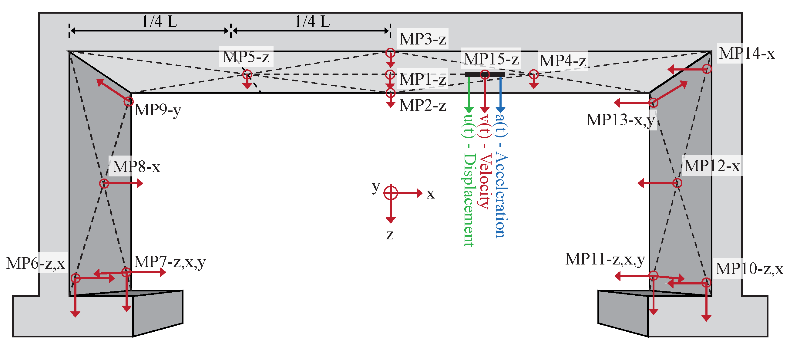
The concept incorporates 22 geophones for the clear identification of the first three eigenmodes, including bending and torsional modes, as well as rigid body modes and abutment movements. The arrangement is illustrated in Figure 8. To ensure the continuous operation of the railway line during measurements, the entire measurement setup was installed beneath the superstructure without any artificial excitation of the structure. As all four bridges have a similar structure and design, identical setups were used for all measurements.

4.2. Evaluation and Assessment

The following description and identification of the dynamic characteristics are given as an example for bridge 12,842.

4.2.1. Description of the Structure

Figure 9 shows the analysed concrete portal frame bridge, with a half-frame configuration and a length of 17 m. The bridge was constructed in 2003 on a shallow foundation. Multichannel analysis of surface waves (MASW) [41] was used to determine the shear wave velocities $V_S$ at the foundation level ($V_S\approx 358$ m/s). The material properties of the backfill (cement-stabilised wedge with $V_{S,K}\approx 1000$ m/s) and the adjacent soil layers (coarse-grained soils with $V_{S,H}\approx 300$ m/s) were assumed.

The superstructure comprises five precast concrete elements (B45) cast on-site with additional in situ concrete (B35) to form a monolithic frame. The abutment walls are followed by wing walls with an opening angle of approximately 45°. The track and road intersect at 90°. Above the in situ concrete are two layers of bitumen sealant, followed by a tray of reinforced concrete (B35) and the slab track.

4.2.2. Identification of Natural Frequencies

To determine the bending and torsional modes, MP1 and MP2 are considered. Derived from the averaged ambient frequency spectra (FFT) shown in Figure 10, the resulting eigenfrequencies are obtained and documented in Table 2. Higher modes were analysed but are not of interest in the following.

For a deeper understanding, the representation of the eigenmodes using Artemis is also included in Figure 10. In contrast, OMA reveals the uncertainty of the first bending eigenfrequency, denoted by $f_1$, where it manifests as either $9.4$ Hz (as identified in the stable mode by stochastic subspace identification) or $9.9$ Hz (as indicated in the Singular Value Decomposition spectrum), depending on the methodology applied.

As a consequence of the averaging process applied to the windowed frequency spectra in the ambient time signal analysis, nearby peaks are smoothed out, revealing only diffuse plots. The indeterminate nature of the initial bending eigenfrequency ($9.4$ Hz $<f_1<10.1$ Hz) remains apparent in the frequency spectrum resulting from pulse excitation (Figure 11). In this case, the effect of averaging is reduced. Furthermore, the uncertainty in the natural frequency is evident in the continuous wavelet transformation (CWT) [50], where the signal characteristics are combined into a representation that is both frequency- and time-dependent (Figure 11b).

In this scenario, the initial bending eigenfrequency defies definitive assignment to a single frequency, with the abutments appearing to play a predominant role, as indicated by a slight counter-phase of the abutment on the “Ingolstadt” side in the OMA. This can lead to divergent structural stiffening due to a phase shift at about ≈10 Hz. The stiffening phenomenon due to counter-phase vibrating foundations is discussed in [51].

4.2.3. Identification of Modal Damping

Modal damping is determined by the integration line of the peaks in the decay curve, as shown in Figure 11a. The damping ratio is evaluated using the mean value of several excitation points.

Figure 11. Analysis of modal damping on the basis of the integrated decay curves in a quiet environment with soft impacts. (a) Time domain, (b) CWT, (c) frequency spectrum.

Figure 11. Analysis of modal damping on the basis of the integrated decay curves in a quiet environment with soft impacts. (a) Time domain, (b) CWT, (c) frequency spectrum.

The evaluation of small amplitudes induced by pulse excitation requires an undisturbed environment (verified by continuous wavelet transform) and a finely tuned measurement chain. In this case, the dissipation mechanisms turn out to be comparable to those observed for larger energy inputs, such as harmonic excitation or train crossings (not further explained). Considering the undisturbed environment, the four evaluation points result in a damping ratio of $\zeta \approx$ 6.1%, matching to the first natural frequency. In comparison, the damping is calculated to be $\zeta =6.3$% using the stochastic subspace identification algorithm implemented in the Artemis.

In addition, damping was characterised on the basis of train crossings. Here, it is important to use the correct reference frequency. In this case, the 4-fold of the base train excitation is in the range of the natural frequency ($4\times 2.5$ Hz), and therefore, the modal damping can be accurately determined to be ${\zeta }_{train}=6.3$–$7\%\approx {\zeta }_{impulse}$.

The assessment of damping ratios for higher modes follows a similar methodology, although a detailed description is omitted here.

4.3. Dynamic Characteristics of In Situ Testing

A comprehensive summary of the collected results from the entire in situ test is presented below in Table 2. The evaluation of the results for the remaining three bridges follows the methodology outlined above.

Table 2. Summary of the studied bridges and their dynamic characteristics.

Bridge	L [m]	${\mathit{f}}_1$ [Hz]	${\mathit{f}}_2$ [Hz]	${\mathit{\zeta }}_1$ [%]	${\mathit{V}}_{\mathit{s}}$ [m/s]	Limitation
		Ambient	Ambient	Mean		${\mathit{a}}_{\mathbf{0}}$
12,842	17	10.1	14.7	6.4	358	$0.90<a_{0,G}$
12,836	17	10.1	14.9	5.9	485	$0.66<a_{0,G}$
12,829	9.5	21.8	25.7	10.9	246	$2.85>a_{0,G}$
13,871	9.5	21.3	25.6	11	600	$1.08>a_{0,G}$

Table 2. Summary of the studied bridges and their dynamic characteristics.

Bridge	L [m]	${\mathit{f}}_1$ [Hz]	${\mathit{f}}_2$ [Hz]	${\mathit{\zeta }}_1$ [%]	${\mathit{V}}_{\mathit{s}}$ [m/s]	Limitation
		Ambient	Ambient	Mean		${\mathit{a}}_{\mathbf{0}}$
12,842	17	10.1	14.7	6.4	358	$0.90<a_{0,G}$
12,836	17	10.1	14.9	5.9	485	$0.66<a_{0,G}$
12,829	9.5	21.8	25.7	10.9	246	$2.85>a_{0,G}$
13,871	9.5	21.3	25.6	11	600	$1.08>a_{0,G}$

A comparison of the measured dynamic characteristics clearly shows the pronounced similarity in the eigenfrequencies of structurally identical bridge pairs despite variations in soil stiffness. The robust eigenfrequencies emphasise the prevalence of structural stiffness as the dominant factor influencing the natural frequency of portal frame bridges, superseding the effects of the (S)SSI. Analogous results are supported by numerical investigations presented in [12].

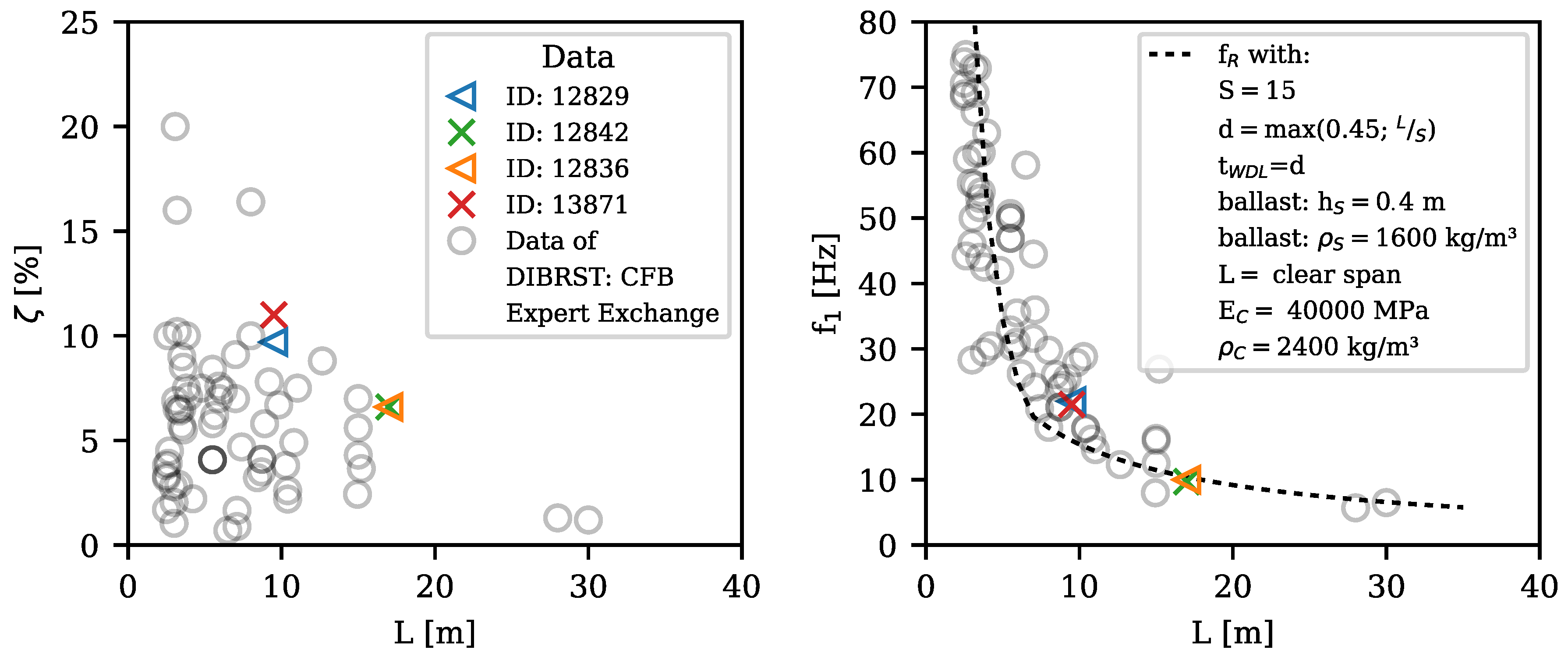
In addition, the results are compared with the data collection of the “Railway bridge dynamics DIBRST: concrete frame bridges—Expert Exchange” [52] in Figure 12. The measured parameters fit well with the data collection.

It is evident that the natural frequencies show minimal deviation from the analytical natural frequency of the frame $f_R$. This frequency is directly related to the stiffness of the superstructure and consequently influences the normative deflection criterion. The tendency of the bridge to have a natural frequency higher than $f_R$ is due to the stiffening effects induced by the backfill and abutment walls, which are not included in the frame formula. A wide range of damping ratios is observed, with the range appearing more extensive for shorter bridges. However, no general principle can be derived for longer spans due to the limited data set. The variability in damping ratios is not surprising, as the (S)SSI, rather than the structure itself, determines the resulting damping characteristics.

5. Comparison of Calculation and Reality

In the following section, the results of the examined bridges are compared with the presented Calculation Model. In order to explain the modelling approach, the model will be illustrated using the example of bridge 12,842.

5.1. Assumptions and Calculation

Primarily, the distinction between static and dynamic bedding approaches is delineated in the context of the portal frame bridge, exemplified by a sample calculation.

According to the documentation, the soil stiffness is given by $E_s=80$–140 MN/m²;. As a first approximation, the static bedding is calculated using the formula $k_s\approx \frac{E_s}{f_{\mathrm{shape}}b}$, as described in [53]. The shape factor $f_{\mathrm{shape}}$ depends on the length-to-width ratio of the footing. In the specific scenario considered, characterised by an average stiffness and an estimated length-to-width ratio, the static bedding is determined according to Equation (35).

$$\begin{array}{cc}\hfill k_s& \approx \frac{110\mathrm{MN}/{\mathrm{m}}^2}{1.4\times 5.5\mathrm{m}}=14.29{\mathrm{MN}/\mathrm{m}}^3\hfill \\ \hfill & \mathrm{with}\hfill \\ \hfill & l=b_T=15.34\mathrm{m};b=b_F=5.5\mathrm{m};f_{\mathrm{shape}}=1.4\hfill \end{array}$$

(35)

However, in the dynamic bedding calculation, neglecting the “trench” and “wall” effects, the equivalent spring stiffness is determined using Equation (15).

$$\begin{array}{cc}\hfill K_{0,z}& =\frac{2Ga}{1-\nu }\left(0.73+1.54{\left(\frac{b}{a}\right)}^{0.75}\right)·I_{Trench}·I_{Wall}=8108.8\mathrm{MN}/\mathrm{m}\hfill \\ \hfill I_{Trench}& =I_{Wall}=1\hfill \\ \hfill & \mathrm{with}\hfill \\ \hfill & a=b_T/2=7.67\mathrm{m},b=b_F/2=2.75\mathrm{m},D_1=1.43\mathrm{m},\hfill \\ \hfill & D_2=6.5\mathrm{m},A_B=84.37{\mathrm{m}}^2;G=256.33\mathrm{MPa};\hfill \\ \hfill & {\rho }_B=2000\mathrm{kg}/{\mathrm{m}}^3;V_S=358\mathrm{m}/\mathrm{s}\left(\mathrm{MASW}\right);\nu =0.3\left(\mathrm{assumption}\right)\hfill \end{array}$$

Considering the foundation area $A_B$, the equivalent bedding is determined to be 96.11 MN/m³, an increase of approximately 6.7 times compared to the static approach. The density and shear wave velocity values are based on the MASW method report [54]. Furthermore, if the lateral bedding effects are considered, the vertical spring stiffness, including $I_{trench,1–2}$ and $I_{wall,1–2}$, is calculated as $K_{0,z,emb}$ = 12,585.9 MN/m.

$$\begin{array}{cc}\hfill I_{Trench,1–2}& =1.0+\frac{1}{21}\frac{1.43+6.5}{2.75}\left(1+\frac{4}{3}\times \frac{2.75}{7.67}\right)=1.2\hfill \\ \hfill I_{Wall,1–2}& =1+0.19{\left(\frac{(1.43+6.5)\times 15.34)}{5.5\times 13.34}\right)}^{2/3}=1.29\hfill \end{array}$$

The ageing effects of concrete are accounted for in the material approach, resulting in an increase in Young’s modulus. As required by the Model Code 2010 [55], an increase of 19% is observed. When applied to the frequency/stiffness relationship, this enhancement in Young’s modulus results in the corresponding stiffening of the eigenfrequency by approximately 4.4%. While analogous increases in Young’s modulus are often reported in the literature, these cases are often associated with “dynamic stiffness” rather than concrete ageing [14,56]. In contrast, research by Heiland asserts that stiffening effects attributed to dynamic loading have only a minor effect on concrete stiffness, with concrete ageing being the main contributor [57].

The numerical model represents the bridge structure by both C3D8 and C3D10 elements. The backfill (C3D8) is rigidly connected to the bridge. The caps and the trough of the slab track, which are characterised by continuous reinforcement in the transverse direction, are assumed to have a stiffness of 20%. In addition, a material damping of 1.5% is attributed to the subsoil.

5.2. Results

The determined natural frequencies, their corresponding eigenmodes and the associated damping ratios show substantial agreement with the results derived from the in situ test, as shown in

Table 3. Comparison of the numerical and in situ measurement results regarding the dynamic characteristics for bridge 12,842.

	${\mathit{f}}_1$ [Hz]/$\mathit{\zeta }$ [%]	${\mathit{f}}_2$ [Hz]	${\mathit{f}}_3$ [Hz]	${\mathit{f}}_4$ [Hz]
Calculation Model	9.9/6.9	13.8	25	28.3
In situ test (ambient)	10.1/6.4	14.7	25	28
Deviation [%]	2/7	6	0	1

. In particular, the discrepancies highlighted in Section 3 have been significantly reduced.

An examination of the deviations in Table 3 shows that the first torsional mode has a more pronounced measured deviation than the other eigenmodes. Studying the eigenmodes in Figure 13, it can be seen that the second mode has more curvature proportions in the abutment regions, particularly in the transverse direction, than the third mode. Consequently, the in situ stiffnesses of the transverse contribution exceed those obtained numerically.

5.3. Summary of the Dynamic Characteristics

The overall results in

Table 4. Comparison of the modal characteristics of the examined frame bridges.

Bridge	L [m]	${\mathit{f}}_1$ [Hz]	${\mathit{f}}_2$ [Hz]	${\mathit{\zeta }}_1$ [%]	${\mathit{a}}_0$
		Numeric/In Situ	Numeric/In Situ	Numeric/In Situ
12,842	17	9.9/10.1	13.8/14.7	6.9/6.4	$0.90<a_{0,G}$
12,836	17	10/10.1	13.8/14.9	4.2/5.9	$0.66<a_{0,G}$
12,829	9.5	22.4/21.8	24.8/25.7	8.5/10.9	$2.85>a_{0,G}$
13,871	9.5	23.7/21.3	25.5/25.6	5.3/11	$1.08>a_{0,G}$

show good agreement, especially with respect to the natural frequencies. Notably, as demonstrated in both 12,842 and 12,836, the first eigenmode achieves a high degree of agreement, while the second eigenmode shows a marginal discrepancy.

Following this trend, the results for 13,871 show excellent agreement in the second eigenmode but a slight overestimation in the first eigenmode. This observed discrepancy suggests an inadequate representation of the lateral stiffnesses, possibly due to the specific structure of the slab track.

The predicted damping ratios for the bridges are very close to the measured values. Unexpectedly, bridge 12,829, characterised by $a_0=2.85>1$, also gives relatively accurate prediction results. However, it is important to note that reaching the application limit does not necessarily lead to poor predictions, as the shape of the impedance function for twin foundations has a strongly oscillatory character (Figure 3).

Furthermore, the Calculation Model for 13,871 shows a notable disparity in the damping ratios. This particular bridge has a directly adjacent retaining wall on one side, located in the transition zone between the railway and motorway bridges, at a distance of approximately 15 m. The omission of this additional interaction in the model explains the increased discrepancies observed in the predictions.

6. Summary and Outlook

This paper highlights the significant influence of the structure–soil–structure interaction (SSSI) on the soil–structure interaction (SSI) and resultant (radiation) damping for concrete portal frame bridges. To simplify engineering calculations, the SSSI’s dynamic shear wave interference can be minimised by setting application limits. This ensures the reliability and robustness of the presented numerical Calculation Model, which uses a special technique incorporating quasi-static dynamic stiffnesses and damping coefficients of arbitrarily shaped rigid foundations to model the SSI.

The validation of the Calculation Model and the comparative in situ investigation of four concrete portal frame bridges on the Nuremberg–Munich high-speed line show a good agreement in the dynamic characteristics. In addition, this study highlights the importance of structural stiffness as the dominant factor influencing natural frequencies.

Given the primary correlation between structural stiffness and natural frequencies, the prediction of modal shapes remains robust even when application limits are exceeded. In terms of damping, compliance with the proposed application limit emerges as a critical factor. Adherence to this limit effectively excludes the influence of the SSSI and represents a conservative scenario. Conversely, exceeding the limit can lead to noticeable differences in the damping determination, but interestingly, in certain cases, it can also lead to accurate predictions. The oscillatory nature of the impedance function proves to be a key factor in this regard.

Further research efforts have the potential to refine the proposed application limits. In particular, a deeper investigation and explanation of the effects and implications of the SSSI are required. The development of standardised impedance functions for common foundation geometries would be a significant step forward.

The stiffness interactions between the slab track and the bridge superstructure are currently unclear and require additional investigation for a more complete understanding.

References

- ERRI D214. Rail Bridges for Speeds > 200 km/h. Final Report. Part (a): Abschlussbericht; Synthesis of the Results of D 214 Research; European Rail Research Institute: Utrecht, The Netherlands, 1999. [Google Scholar]
- Baeßler, M. Lageveränderungen des Schottergleises Durch Zyklische und Dynamische Beanspruchungen. Ph.D. Thesis, Technische Universität Berlin, Berlin, Germany, 2008. [Google Scholar]
- Deutsches Institut für Normung e.V. (DIN). Einwirkungen auf Tragwerke-Teil 2: Verkehrslasten auf Brücken; DIN EN 1991-2:2010-12, Eurocode 1; Beuth Verlag GmbH: Berlin, Germany, 2010. [Google Scholar] [CrossRef]
- DB Netz AG. Eisenbahnbrücken (und Sonstige Ingenieurbauwerke) Planen, Bauen und Instand Halten; RIL 804; DB Netz AG: Berlin, Germany, 2013. [Google Scholar]
- Kohl, A.M.; Vospernig, M.; Kwapisz, M.; Grunert, G.; Firus, A.; Schneider, J. Neues Hochgeschwindigkeitslastmodell für Eisenbahnbrücken—Teil 2: Auswahl repräsentativer Fahrzeuge. In Baudynamik; VDI-Berichte, VDI Verlag GmbH: Düsseldorf, Germany, 2022; pp. 81–94. [Google Scholar] [CrossRef]
- Kohl, A.M.; Clement, K.D.; Schneider, J.; Firus, A.; Lombaert, G. An investigation of dynamic vehicle-bridge interaction effects based on a comprehensive set of trains and bridges. Eng. Struct. 2023, 279, 115555. [Google Scholar] [CrossRef]
- Hirzinger, B.; Adam, C.; Salcher, P. Dynamic response of a non-classically damped beam with general boundary conditions subjected to a moving mass-spring-damper system. Int. J. Mech. Sci. 2020, 185, 105877. [Google Scholar] [CrossRef]
- Zangeneh, A.; Svedholm, C.; Andersson, A.; Pacoste, C.; Karoumi, R. Identification of soil-structure interaction effect in a portal frame railway bridge through full-scale dynamic testing. Eng. Struct. 2018, 159, 299–309. [Google Scholar] [CrossRef]
- Zangeneh Kamali, A. Dynamic Soil-Structure Interaction Analysis of High-Speed Railway Bridges: Efficient Modeling Techniques and Experimental Testing: Doctoral Thesis in Structural Engineering and Bridges; TRITA-ABE-DLT; KTH Royal Institute of Technology: Stockholm, Sweden, 2021; Volume 2121. [Google Scholar]
- Bigelow, H.; Pak, D.; Hoffmeister, B.; Feldmann, M.; Seidl, G.; Petraschek, T. Soil-structure interaction at railway bridges with integral abutments. Procedia Eng. 2017, 199, 2318–2323. [Google Scholar] [CrossRef]
- Marx, S.; Geißler, K. Erfahrungen zur Modellierung und Bewertung von Eisenbahnbrücken mit Resonanzrisiko. Stahlbau 2010, 79, 188–198. [Google Scholar] [CrossRef]
- Heiland, T.; Aji, H.D.; Wuttke, F.; Stempniewski, L.; Stark, A. Influence of soil-structure interaction on the dynamic characteristics of railroad frame bridges. Soil Dyn. Earthq. Eng. 2023, 167, 107800. [Google Scholar] [CrossRef]
- Heiland, T.; Hägle, M.; Triantafyllidis, T.; Stempniewski, L.; Stark, A. Stiffness contributions of ballast in the context of dynamic analysis of short span railway bridges. Constr. Build. Mater. 2022, 360, 129536. [Google Scholar] [CrossRef]
- Reiterer, M.; Bruschetini-Ambro, S.Z. Dynamik von Eisenbahnbrücken: Diskrepanz zwischen Messung und Berechnung. Bauingenieur 2019, 94, 9–21. [Google Scholar] [CrossRef]
- Dobry, R.; Gazetas, G. Dynamic Response of Arbitrarily Shaped Foundations. J. Geotech. Eng. 1986, 112, 109–135. [Google Scholar] [CrossRef]
- Studer, J.A.; Koller, M.G.; Laue, J. Bodendynamik: Grundlagen, Kennziffern, Probleme und Lösungsansätze; Springer: Berlin/Heidelberg, Germany, 2008. [Google Scholar] [CrossRef]
- Vrettos, C. Bodendynamik. In Grundbau-Taschenbuch; Witt, K.J., Ed.; Wiley-VCH Verlag GmbH & Co. KGaA: Weinheim, Germany, 2008; pp. 451–500. [Google Scholar] [CrossRef]
- Lysmer, J. Vertical Motion of Rigid Footings; University of Michigan: Ann Arbor, MI, USA, 1965. [Google Scholar]
- Wolf, J.P. Foundation Vibration Analysis Using Simple Physical Models; Prentice Hall, Inc.: Englewood Cliffs, NJ, USA, 1994. [Google Scholar]
- Gazetas, G. Foundation Vibrations. In Foundation Engineering Handbook; Fang, H.Y., Ed.; Springer: Boston, MA, USA, 1991; pp. 553–593. [Google Scholar] [CrossRef]
- Pais, A.; Kausel, E. Approximate formulas for dynamic stiffnesses of rigid foundations. Soil Dyn. Earthq. Eng. 1988, 7, 213–227. [Google Scholar] [CrossRef]
- Petersen, C. Dynamik der Baukonstruktionen; Springer: Berlin/Heidelberg, Germany, 2013. [Google Scholar]
- Deutsche Gesellschaft für Geotechnik e.V. Empfehlungen des Arbeitskreises “Baugrunddynamik”, 1st ed.; Ernst, Wilhelm & Sohn: Berlin, Germany, 2017. [Google Scholar]
- Triantafyllidis, T. Dynamic stiffness of rigid rectangular foundations on the half-space. Earthq. Eng. Struct. Dyn. 1986, 14, 391–411. [Google Scholar] [CrossRef]
- Wong, H.L.; Luco, J.E. Dynamic response of rigid foundations of arbitrary shape. Earthq. Eng. Struct. Dyn. 1976, 4, 579–587. [Google Scholar] [CrossRef]
- Gazetas, G. Analysis of machine foundation vibrations: State of the art. Int. J. Soil Dyn. Earthq. Eng. 1983, 2, 2–42. [Google Scholar] [CrossRef]
- Eringen, A.C. Elastodynamics, Volume 2: Linear Theory; Elsevier Science: Burlington, MA, USA, 1975. [Google Scholar]
- Gazetas, G.; Dobry, R.; Tassoulas, J.L. Vertical response of arbitrarily shaped embedded foundations. J. Geotech. Eng. 1985, 111, 750–771. [Google Scholar] [CrossRef]
- Aji, H.D.B. Hybrid BEM-FEM for 2D and 3D Dynamic Soil-Structure Interaction Considering Arbitrary Layered Half-Space and Nonlinearities. Ph.D. Thesis, CAU, Kiel, Germany, 2023. [Google Scholar] [CrossRef]
- Studer, J.A.; Koller, M.G.; Laue, J. Bodendynamik; Springer: Berlin/Heidelberg, Germany, 2007. [Google Scholar]
- Stempniewski, L.; Haag, B. Baudynamik-Praxis: Mit Zahlreichen Anwendungsbeispielen, 1st ed.; Bauwerk-Verl.: Berlin, Germany, 2010. [Google Scholar]
- Mulliken, J.S.; Karabalis, D.L. Discrete model for dynamic through-the-soil coupling of 3-D foundations and structures. Earthq. Eng. Struct. Dyn. 1998, 27, 687–710. [Google Scholar] [CrossRef]
- Wolf, J.P.; Meek, J.W. Insight on 2D- versus 3D-modelling of surface foundations via strength-of-materials solutions for soil dynamics. Earthq. Eng. Struct. Dyn. 1994, 23, 91–112. [Google Scholar] [CrossRef]
- Aji, H.D.B.; Basnet, M.B.; Wuttke, F. Numerical modelling of the dynamic behavior of an integral bridge via coupled BEM-FEM. In Proceedings of the 16. D-A-CH Tagung Erdbebeningenieurwesen & Baudynamik, Innsbruck, Austria, 26–27 September 2021. [Google Scholar]
- Aji, H.D.B.; Wuttke, F.; Dineva, P. 3D hybrid model of foundation-soil-foundation dynamic interaction. ZAMM J. Appl. Math. Mech. Z. Angew. Math. Mech. 2021, 101, e202000351. [Google Scholar] [CrossRef]
- Hackenberg, M. A Coupled Integral Transform Method-Finite Element Method Approach to Model the Soil-Structure-Interaction. Ph.D. Thesis, Technische Universität München, München, Germany, 2017. [Google Scholar]
- Wolf, J.P. Soil-structure-interaction analysis in time domain. Nucl. Eng. Des. 1989, 111, 381–393. [Google Scholar] [CrossRef]
- Vucetic, M. Cyclic Threshold Shear Strains in Soils. J. Geotech. Eng. 1994, 120, 2208–2228. [Google Scholar] [CrossRef]
- Wichtmann, T.; Triantafyllidis, T. Dynamische Steifigkeit und Dämpfung von Sand bei kleinen Dehnungen. Bautechnik 2005, 82, 236–246. [Google Scholar] [CrossRef]
- Abaqus CAE 2020; Dassault Systemes Simulia Corporation. Available online: https://www.3ds.com/products/simulia/abaqus (accessed on 15 January 2024).
- Dal Moro, G. Surface Wave Analysis for Near Surface Applications; Elsevier: Amsterdam, The Netherlands, 2015. [Google Scholar]
- Dal Moro, G. Efficient Joint Analysis of Surface Waves and Introduction to Vibration Analysis; Springer International Publishing AG: Cham, Switzerland, 2020. [Google Scholar]
- Nasdala, L. FEM-Formelsammlung Statik und Dynamik; Springer: Wiesbaden, Germany, 2015. [Google Scholar] [CrossRef]
- Stollwitzer, A.; Fink, J. Verfahren zur Reduktion der Ergebnisstreuung zur Ermittlung realistischer Lehr’scher Dämpfungsmaße von Eisenbahnbrücken—Teil 2: Methoden im Zeitbereich. Bauingenieur 2022, 97, 341–352. [Google Scholar] [CrossRef]
- Stollwitzer, A.; Fink, J.; Mohamed, E. Verfahren zur Reduktion der Ergebnisstreuung zur Ermittlung realistischer Lehr’scher Dämpfungsmaße von Eisenbahnbrücken—Teil 1: Methoden im Frequenzbereich. Bauingenieur 2022, 97, 153–164. [Google Scholar] [CrossRef]
- Virtanen, P.; Gommers, R.; Oliphant, T.E.; Haberl, M.; Reddy, T.; Cournapeau, D.; Burovski, E.; Peterson, P.; Weckesser, W.; Bright, J.; et al. SciPy 1.0: Fundamental algorithms for scientific computing in Python. Nat. Methods 2020, 17, 261–272. [Google Scholar] [CrossRef] [PubMed]
- Python 3.; Python Software Foundation. Available online: https://www.python.org/ (accessed on 15 January 2024).
- ARTeMIS Modal; Structural Vibration Solutions A/S, Aalborg East, Denmark, 2021. Python 3. Available online: https://www.svibs.com/ (accessed on 15 January 2024).
- Brincker, R.; Andersen, P. Understanding Stochastic Subspace Identification. In Proceedings of the Conference Proceedings: IMAC-XXIV: A Conference & Exposition on Structural Dynamics, St. Louis, MO, USA, 30 January–2 February 2006. [Google Scholar]
- Mallat, S.G. A Wavelet Tour of Signal Processing: The Sparse Way, 3rd ed.; Elsevier: Amsterdam, The Netherlands; Academic Press: Boston, MA, USA, 2009. [Google Scholar]
- Heiland, T.; Thomas, L.; Galiazzo, M.; Stempniewski, L.; Stark, A. Auswirkungen der ebenen Boden-Bauwerk-Interaktion auf die Eigenfrequenz von Eisenbahnrahmenbrücken. Bauingenieur 2022, 97, 141–152. [Google Scholar] [CrossRef]
- CEN TC250. CEN TC250/TR xxxxx:2023_InBridge4EU, Scheduled for Publication. Available online: https://eurocodes.jrc.ec.europa.eu/policies-standards/centc250-structural-eurocodes (accessed on 15 January 2024).
- Goris, A. (Ed.) Bautabellen für Ingenieure: Mit Berechnungshinweisen und Beispielen, 20th ed.; Werner: Neuwied, Germany, 2012. [Google Scholar]
- Korda, F.; Mistler, M. Brückenmessungen bei Nürnberg: Dokumentation der Brückenmessung und Untersuchung der dynamischen Bodeneigenschaften; Baudynamik Heiland & Mistler GmbH: Bochum, Germany, 2022. [Google Scholar]
- FIB. Model Code for Concrete Structures 2010: Model Code 2010; Ernst & Sohn Publishing House: Berlin, Germany, 2013. [Google Scholar] [CrossRef]
- Ziegler, A. Bauwerksdynamik und Erschütterungsmessungen; Springer: Wiesbaden, Germany, 2017. [Google Scholar] [CrossRef]
- Heiland, T.; Hofmann, F.; Stempniewski, L. Eine Grenzwertbetrachtung über die Auswirkungen des dynamischen E-Moduls auf die Eigenfrequenzen bei Eisenbahnrahmenbrücken. In Proceedings of the 17. D-A-CH Tagung Erdbebeningenieurwesen & Baudynamik, Online, 16–17 September 2021. [Google Scholar]
Figure 1.
(a) A massless rigid square foundation under harmonic excitation in a trench on a homogeneous elastic half-space, (b) the system sketch, (c) the impedance function for and data according to the literature [17,19,20,21].
Figure 2.
(a) Illustration of the SSI of a concrete portal frame bridge depending on the numerical solution: (b) using the direct method; (c) using the substructure method.
Figure 3.
Impedance functions of the massless rigid abutment; numerical results are based on the hybrid method according to [12]. (a) Real part, (b) imaginary part, (c) visualisation of the systems.
Figure 4.
Calculation Model of a portal frame bridge. (a) Problem description; (b) system sketch.
Figure 5.
A comparison of the dynamic characteristics of the frame using the hybrid modelling technique and the Calculation Model when varying the span: (a) damping ratio; (b) natural frequency.
Figure 6.
Comparison of the dynamic characteristics on the 17m frame using the hybrid modelling technique and the Calculation Model when varying the abutment width: (a) damping ratio; (b) natural frequency.
Figure 7.
General view of concrete portal frame bridge 12,842.
Figure 8.
Sketch with illustration and orientation of the measurement points.
Figure 9.
Longitudinal section of the bridge [DB Netz AG] and associated soil profile.
Figure 10.
Evaluation of the natural frequencies and associated modal shapes of frame bridge 12,842. (a) Time history of the ambient vibration velocity and averaged frequency spectrum. (b) Evaluation of 1st eigenmode. (c) Evaluation of 2nd eigenmode.
Figure 12.
Dynamic characteristics of the investigated frame bridges compared to the data collection of the DIBRST [52].
Figure 13.
Illustration of the numerically determined first four eigenmodes using Abaqus.