Ensemble Empirical Mode Decomposition Granger Causality Test Dynamic Graph Attention Transformer Network: Integrating Transformer and Graph Neural Network Models for Multi-Sensor Cross-Temporal Granularity Water Demand Forecasting

Abstract

Accurate water demand forecasting is crucial for optimizing the strategies across multiple water sources. This paper proposes the Ensemble Empirical Mode Decomposition Granger causality test Dynamic Graph Attention Transformer Network (EG-DGATN) for multi-sensor cross-temporal granularity water demand forecasting, which combines the Transformer and Graph Neural Networks. It employs the EEMD–Granger test to delineate the interconnections among sensors and extracts the spatiotemporal features within the causal domain by stacking dynamical graph spatiotemporal attention layers. The experimental results demonstrate that compared to baseline models, the EG-DGATN improves the MAPE metrics by 2.12%, 4.33%, and 6.32% in forecasting intervals of 15 min, 45 min, and 90 min, respectively. The model achieves an R2 score of 0.97, indicating outstanding predictive accuracy and exceptional explanatory power for the target variable. This research highlights significant potential applications in predictive tasks within smart water management systems.

1. Introduction

As urbanization accelerates, establishing intelligent water demand forecasting systems has become a crucial component of smart city development. The precision of water demand forecasting plays a fundamental role in constructing such intelligent systems, as it enables minimizing resource wastage caused by redundant water supply, guiding efficient water distribution across different geographic units, and providing valuable data for leak detection [1,2]. These applications require developing a method for water demand forecasting that is efficient, accurate, and capable of integrating multi-sensor data across varying temporal granularities.

In recent decades, predicting water demand in urban areas has become a major topic of interest in academic research. In early research, statistical methods were widely applied to water demand forecasting due to their simplicity and interpretability. Oliveira et al. applied the harmony search algorithm to optimize the ARIMA model for forecasting in a specific area [3]. Meanwhile, Guo et al. employed VAR to incorporate factors affecting the forecast outcomes, particularly for short-term agricultural irrigation water forecasting [4]. In contrast to these statistical-based methods, machine learning approaches handle complex nonlinear relationships inherent in data and have demonstrated substantial advancements in forecasting. For instance, Li et al. combined the RandomForest model with linear regression to achieve water consumption forecasting at fixed time intervals [5]. Candelieri et al. designed parallel global optimization algorithms to optimize SVM parameters to solve complex water demand forecasting [6]. While these methods can depict nonlinear relationships, their models rely on intricate feature engineering.

Deep learning models exhibit greater versatility than machine learning models as they can autonomously learn the relationships between features. Consequently, more researchers are considering deep learning for water demand forecasting applications. Mu et al. utilized the LSTM model for short-term urban water demand forecasting [7]. In contrast, Zanfei et al. designed an ensemble model incorporating simple recurrent networks (SRNNs), LSTM, and gated recurrent unit networks (GRU), applied to water demand forecasting at 1 h and 24 h intervals [8]. These methods mainly focus on analyzing the temporal autocorrelation within individual series. This practice significantly diverges from the reality of multiple sensors contributing to complex multivariate time series in real water supply networks. Researchers have aggregated sensor data for synchronous prediction to align with practical water network scenarios. For instance, Hu et al. combined two-dimensional convolution with Bi-LSTM models for synchronous forecasting across various sensor data over time and space, thereby improving the model accuracy [9]. However, this modeling approach relies on processed grid data, reducing the model’s versatility. Due to the excellent performance of graphical convolutional neural networks (GCN) in handling tasks involving correlations among multiple sensors, researchers have applied them to water demand forecasting. For instance, Lin et al. utilized the GraphWave network to effectively enhance the accuracy of short-term water demand forecasting in water supply networks by optimizing the topological features of objects and extracting spatiotemporal features [10]. These methods achieve spatial information aggregation using graph convolutional neural networks and still rely on RNN models stacking multiple predictions in time to attain multi-granularity prediction; this inevitably creates the problem of error stacking and gradient explosion.

The Transformer model utilizes self-attention mechanisms to capture temporal relationships between different time steps, avoiding the error propagation issues associated with sequential processing. This has led to its widespread application in various scenarios of time series prediction tasks [11]. For instance, Nie et al. applied the Transformer model to the field of traffic flow prediction, and the independence of location coding is utilized to improve long-time series prediction performance [12]. Combining the Transformer model with graph convolutional neural networks for spatiotemporal prediction has gradually become the focus of academic research. For example, Xu et al. combined Transformer with GCN, utilizing attention mechanisms to learn multiple sensors’ temporal and spatial dependencies separately, thereby improving the accuracy and efficiency of predictions at different time granularities [13]. To further enhance the accuracy of spatiotemporal predictions, many scholars propose utilizing adjacency matrices containing richer information to assist the model. For example, Fang et al. introduced the Dynamic Time Warping (DTW) method to generate similarity matrices to help extract information, thereby improving the model’s predictive performance [14]. Jin et al. summarized the performance enhancement of GCN-based spatiotemporal prediction models based on predefined adjacency matrices calculated with different similarities [15]. However, these methods do not jump over the limitations of existing spatiotemporal relations. In statistics, the Granger causality test method is widely applied to analyze the relationship between two-time series. For instance, Tian et al. utilized the Granger causality test method to investigate the correlation between different sectors of Chinese and American stocks, thereby forming a causal relationship network [16]. This facilitates a transition in the analysis of sensor network relationships from a spatial perspective to a causal domain.

Although these methods extend the approach to modeling spatiotemporal sequences, almost all methods use historical and predictive windows for model training, so enhancing the density of information encapsulated within an individual window has been identified as a potent strategy to augment the model’s predictive capabilities. Some scholars proposed decomposing series at the frequency level, employing techniques like Empirical Mode Decomposition (EMD). Combining Empirical Mode Decomposition (EMD) with deep learning models enables the extraction of time patterns across different frequency components in time series data, which may be challenging for models to learn directly from raw data. This method has been applied in various fields. For example, Zhu et al. combined EMD with LSTM to refine the accuracy of long-term deformation prediction for tailings dams, achieving this by aggregating the results from various LSTM model components [17]. Hou et al. designed an EMD-Particle Swarm Optimization-Gaussian process regression combination model, achieving accurate stress forecasting in ultra-high arch dams [18]. The application of EEMD methods in water demand forecasting has been relatively limited.

Overall, despite the good predictive results achieved by existing methods, the following challenges still need to be overcome:

• Existing models that analyze spatiotemporal data often treat spatial and temporal relationships as separate entities. This separation can lead to significant information loss, subsequently diminishing the accuracy of the model’s predictions.
• Furthermore, when dealing with natural scenes, the spatial relationships between sensors might not always be apparent or accessible, complicating the model’s learning process. Consequently, there is a pressing need for innovative graph-building techniques that can facilitate adequate information flow among sensor nodes without relying on predefined spatial relationships.
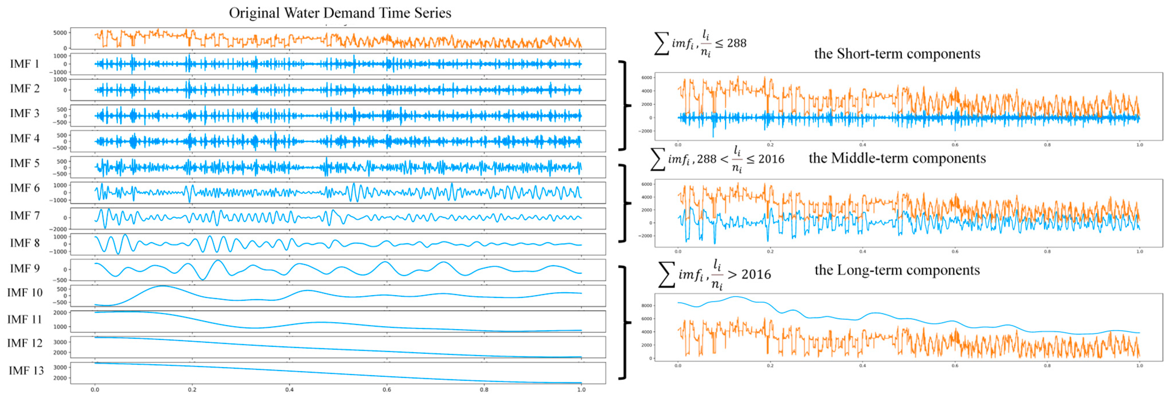
• Additionally, assigning a distinct time series model to each series decomposed using the Empirical Mode Decomposition (EMD) method has proven inefficient. A more streamlined approach is required to fully capitalize on the insights from the decomposed series fully, enhancing the overall model efficiency.

Addressing these challenges, we introduce the Ensemble EMD (EEMD) Granger causality test Dynamic Graph Attention Transformer Network (EG-DGATN) model, intending to improve the accuracy of water demand forecasting tasks for multiple regional geographic units without relying on prior graph structures. Different from other methods, this model imposes no specific constraints on data input and offers the following contributions:

• Enhanced Temporal Information Fusion and Causal Relationship Exploration in Sensor Networks. We utilize EEMD–Granger causality testing to integrate additional temporal information within a fixed time dimension, circumventing the need for model stacking inherent in traditional approaches and facilitating a deeper investigation into the causal interplay among sensor networks.
• Optimized Spatial-Temporal Encoding and Synchronized Modeling. By incorporating causal spatiotemporal embeddings into the Transformer architecture, we have refined positional encoding, enabling the EG-DGATN model to synchronize the treatment of spatiotemporal relationships among water demand sensors. This enhancement outperforms traditional models segregating spatial and temporal data, yielding a more comprehensive and precise predictive framework.
• Innovative Dynamic Graph-Optimized Multi-Head Attention Mechanism. We propose a novel dynamic graph multi-head attention mechanism, which regulates the flow of information in the water supply sensor network and achieves efficient information aggregation. Unlike traditional attention mechanisms, it dynamically adjusts attention weights based on real-time data and changes in the sensor network, better capturing and utilizing the temporal-spatial dependencies within water demand data.

The rest of the article is organized as follows. Section 2 provides an overview of the EG-DGATN’s architecture, detailing the EEMD–Granger causal test and the roles of the model’s components. Section 3 reports on the experimental evaluation, where the proposed method is benchmarked against various baseline models to demonstrate its superiority. The final section, Section 4, concludes the paper with a summary of findings and explores several promising applications of the EG-DGATN framework in smart water management systems.

2. Methods

2.1. Objective Description

Given historical water demand monitoring data, the water demand forecasting task involves forecasting the future water demand for each $N$ geographical unit. In this paper, the relationships between the $N$ geographical units are defined as a graph G = (V, E, A), where V represents the sensors corresponding to geographical units, i.e., $\left|V\right|=N$, $E$ is the set of edges, and $A\in {\mathbb{R}}^{N\times N}$ is the adjacency matrix. The historical water demand records of graph $G$ at time $t$ are represented as a graph signal $X_{\left(t\right)}\in {\mathbb{R}}^{N\times 1}$. The EG-DGATN aims to predict $P$ future graph signals using $T$ historical graph signals, as shown in Equation (1):

$$\left[X_{\left(t-T+1\right)},X_{\left(t-T+2\right)},...,X_{\left(t\right)}\right]\stackrel{f\left(·\right)}{\Rightarrow }\left[\acute{X_{(t+1)}},\acute{X_{(t+2)}},...,\acute{X_{(t+P)}}\right]$$

(1)

2.2. Data Preprocessing

The time series is first obtained from different sensors, as shown in Figure 1. To avoid interference from outliers, the series is subjected to Hampel filtering. Subsequently, the filtered data are separately processed to construct the causality matrix and the DTW [14] matrix. The construction process of the causality matrix includes EEMD decomposition, the merging of Intrinsic Mode Functions (IMFs), an Augmented Dickey-Fuller (ADF) stationarity testing, and Granger causality testing [19], resulting in the final causality matrix. Similarly, DTW is applied to compute the similarity matrix for the data. Combining these matrices forms a water demand sensors causal graph, which serves as the output of the data preprocessing process and is fed into the model for computation. The details of this chapter will describe the data preprocessing process.

2.2.1. EEMD and ADFuller Stationarity Test

EMD is an adaptive and efficient technique used to handle time series. Its main contribution is that any complex series can be decomposed into a finite and typically small number of IMF $imf$ and residual $r\left(t\right)$, which are nearly non-overlapping orthogonal components in the frequency domain. The process of EMD is shown in Equation (2):

$$x\left(t\right)={\sum }_i^{k}im{f}_i+r\left(t\right)$$

(2)

To enhance the reductions in mode mixing and improve the noise robustness of the decomposition process, EEMD performs multiple iterations of EMD on a given signal $x\left(t\right)$, introducing different random noises into the signal each time. The $imf$s obtained from each iteration are then averaged to reduce the randomness introduced in a single run, resulting in the final $imfs$.

After EEMD, the original time series is decomposed into IMFs from high to low frequency. This implies that these $imfs$ contain information ranging from short-time scale to long-timescale [16]. Subsequently, the decomposed $imfs$ are reconstructed into three relatively independent components, each carrying different time-scale information. The reconstruction process is illustrated in Equation (3):

$$\left\{\begin{array}{c}{I}_1\left(t\right)=\sum im{f}_i,\frac{l_i}{n_i}\le 288\\ I_2\left(t\right)=\sum im{f}_i,288<\frac{l_i}{n_i}\le 2016\\ I_3\left(t\right)=\sum im{f}_i,\frac{l_i}{n_i}>2016\end{array}\right.$$

(3)

where $I_1\left(t\right)$ represents the short-term component, $I_2\left(t\right)$ represents the middle-term component, and $I_3\left(t\right)$represents the long-term component. $n_i$ is the total number of local extrema detected for each $im{f}_i$, and $l_i$ is the length of $im{f}_i$.

Since the sensor recordings are taken every 5 min, each day consists of 288 time granularities. If the ratio of$l_i$ to $n_i$is below 288, it can be deemed a daily periodicity, suggesting a short-term component. This principle applies to other term components as well.

Since the Granger causality test is only applicable to stationary series, the reconstructed time series components need to undergo the Augmented Dickey–Fuller test for stationarity testing. The process is illustrated in Equation (4):

$$∆y_t=\rho y_{t-1}+\gamma +{\beta }_1\Delta y_{t-1}+{\beta }_2\Delta y_{t-2}+\cdots +{\beta }_p\Delta y_{t-p}+{ϵ}_t$$

(4)

where $∆$ represents the first-order difference, $y_t$ is the value of the time series, $\rho$ is the test statistic, $\gamma$ is the intercept, ${\beta }_1,{\beta }_2, \dots ,{\beta }_p$ are the coefficients of the difference terms, and ${ϵ}_t$ is the introduced white noise. The null hypothesis of the ADF test is that the time series has a unit root, indicating non-stationarity, while the alternative hypothesis is that the series is stationary. During the ADF test, attention is focused on whether the test statistic $\mathsf{\rho }$ is is significant. If the null hypothesis is significantly rejected, it can be concluded that the time series is stationary.

2.2.2. Granger Causality Tests and DTW

According to the Granger causality test [19], given two variables x and y, variable x can be considered to influence variable y in an appropriate statistical sense if the forecasting of the value of y is based on the past values of y and the past values of x is better than the forecasting of the value of y is based only on the past values of y. As in Equation (5), one can test for Granger causality between the two series by constructing binary vector autoregressive models:

$$\left\{\begin{array}{c}{y}_t=\alpha +\sum _{i=1}^m{\beta }_i{y}_{t-i}+\sum _{j=1}^n{\gamma }_j{x}_{t-j}+{\eta }_t\\ y_t=\alpha +{\sum }_{i=1}^m{\beta }_i{y}_{t-i}+{\eta }_t\end{array}\right.$$

(5)

where $x_t$ and$y_t$ are elements of two time series on a uniform time scale. Two autoregressive models are constructed for $y_t$; model 1 includes the causal hypothesis, while model 2 does not. In these models, $\alpha ,\beta ,\mathrm{a}\mathrm{n}\mathrm{d} \gamma$ are the parameters to construct the autoregressive model, and ${\eta }_t$ represents the residual term. The values of m and n, determining the number of lag terms, are selected based on the Bayesian Information Criterion, ultimately determining the maximum lag order as n = 15.

After obtaining the two autoregressive models, the hypothesis that $y_t$ and $x_t$ are not causally related is initially assumed, followed by conducting F-tests on both models [16]. If the calculated p-value of the F-test is less than 0.05, the hypothesis is rejected, indicating that x is the Granger cause of y. The Granger cause can help determine which sensor data can change in time ahead of other sensors’ data changes and impact them; further, it can obtain information on how information flows and propagates through the sensor network, which helps to understand the interconnections between sensors.

The causal network presented in this paper is directly constructed based on the results of the Granger causality test. By setting the significance level of the F-test’s calculated p-value (significance level) to be less than 0.01 as the threshold, a threshold network can be constructed. At each time scale, series are considered nodes, with edges indicating their Granger relationships.

For water demand recorded by different sensors, after undergoing EEMD, the three temporal components, $I_1\left(t\right),I_2\left(t\right),I_3\left(t\right)$, are subjected to Granger causality tests separately with the time series components of other sensors, and the causal matrices for short-term, middle-term, and long-term components, $G_s,G_M,G_L{\in \mathbb{R}}^{N\times N}$, are constructed. A multi-time scale network allows for the exploration of richer information than the original data level and enables more detailed data analysis across multiple time scales. This way, utilizing the decomposed time series avoids modeling each decomposed $imf$ separately, thereby reducing model complexity and allowing subsequent models to learn information from causal spatial-temporal relationships.

The adjacency matrix $G_{DTW}$generated using $DTW$ can supplement the information regarding the relationships between time series. Its generation process is illustrated in Equations (6) and (7) as follows:

$$D\left(i,j\right)=Dist\left(x_i,y_j\right)+min\left(D\left(i-1\right),j\right),D(i,j-1),D(i-1,j-1))$$

(6)

$$G_{DTW}\left(i,j\right)=\left\{\begin{array}{c}1,D\left(X^i,X^j\right)<\epsilon \\ 0,otherwise\end{array}\right.$$

(7)

where the $Dist$ function represents the calculation of the Euclidean distance between two times, $D\left(i,j\right)$ denotes the shortest distance between the subsequent $X=\left(x_1,x_2,x_3,\dots ,x_i\right)$ and $Y=\left(y_1,y_2,y_3,\dots ,y_j\right)$, by which it better reflects the similarity between two time series. $X^i$ denotes the series of sensor $i$. If the $DTW$ calculation of two sequences is less than the threshold$\epsilon$, they are considered to have a neighboring relationship.

2.3. EG-DGATN Model Framework

The framework of the EG-DGATN model is depicted in Figure 2. The model first obtains causal spatiotemporal embeddings of different sensors in different time series. The model stacks Dynamic Graph ST-attention layers to form an encoder and decoder; the encoder generates training window time series representations, and the decoder decodes these representations and populates the prediction window data through the output layer. The detailed description of each component is shown in the following subsections.

2.3.1. Causal Spatiotemporal Embedding

To avoid the accumulation of errors and error propagation commonly observed in long-granularity forecasts in traditional models, the EG-DGATN utilizes the Transformer architecture. The prediction process of Transformer is temporally synchronized, which requires each sensor to be pre-position encoded at different time granularities. To accurately capture the correlation information in the sensor network, we optimize the common positional encoding with causal spatial embedding, achieving synchronous modeling of sensor nodes in both the causal spatial domain and temporal domain. Causal spatiotemporal embedding $STE$ includes both causal spatial embedding $SE$ and temporal embedding $TE$.

To fully embed the sensor space feature in the causal domain, Node2Vec [20] is utilized to perceive the causal space and generate embedding vectors. Node2Vec conducts random walks on the causal-directed matrix and the DTW similarity matrix across three time spans, producing a vector representation for each walk sequence. These vector representations are then aggregated to obtain a comprehensive embedding for each sensor. Furthermore, the embeddings of the causal structures between different sensor sequences learned by Node2Vec on various graph structures are then aggregated. After passing through fully connected (FC) layers. In this way, we enable SE to obtain the causal relationships in the water demand sensor network under different time spans, enriching the information contained therein, as shown in Equation (8).

$$SE=FC\left(concat\left(Node2VectorEncoding(G_s,G_M,G_L,G_{DTW})\right)\right)\in {\mathbb{R}}^{N\times (T+P)\times D}$$

(8)

where $TE$ represents the position of a variable in the entire time steps [12]. $T$ represents the length of the training window, while $P$ represents the size of the prediction window.

Considering the daily, weekly, and seasonal periodicity of water usage, one-hot encoding is performed for the position of the current time step within a day, the position within a week, and the position within a month relative to the entire year, generating${ V}_{time}\in {\mathbb{R}}^{1\times 288}$, $V_{week}\in {\mathbb{R}}^{1\times 7}$, $V_{month}\in {\mathbb{R}}^{1\times 12}$. The process of generating embedding is shown in Equations (9) and (10).

$$TE=unsqueeze\left(FC\right(concat(V_{time},V_{week, }{V}_{month})) \in {\mathbb{R}}^{N\times (T+P)\times D}$$

(9)

$$STE=TE+SE\in {\mathbb{R}}^{N\times (T+P)\times D}$$

(10)

where the unsqueeze function is used to expand the dimensions, aligning the dimensions of time encoding with those of causal space encoding.

By combining $SE$ and $TE$, we enable the transformation of causal spatiotemporal features into more actionable causal spatiotemporal embeddings. This process distinctly identifies the unique position of specific time granularities within the causal spatiotemporal graph across various periods. The $STE$ is divided into two parts in training: the length of the two parts is aligned with the training window $T$ and the prediction window $P$, respectively. The first part will be used as positional coding in the encoder, which is merged with the sequence and then passes through the input layer to the coding stage, ultimately generating the sequence representation. Subsequently, the latter segment is amalgamated with the sequence representation and directed into the Decoder. This step will enable the decoder to forecast the outcome associated with a specific location accurately.

2.3.2. Dynamic Graph ST-Attention Layer

The dynamic graph ST-attention layer is the core component of the EG-DGATN. It dynamically learns the potential relationships in the sensor network by generating dynamic graphs, thus enhancing the effectiveness of aggregating information [21]. While aggregating information, this layer utilizes the multi-head attention mechanism from Transformer to optimize the message-passing mechanism in GCNs to update sensor node information. This layer mainly comprises the sensor network’s first-order neighborhood dynamic graph generation and message-passing processes.

The dynamic graph $A_d$ generation process can be illustrated in Equation (11):

$$\left\{\begin{array}{c}{M}^k=tanh\left(\beta E^k{\Gamma }_{gc}^k\right),k\in \mathrm{1,2}\\ A_d\left(i,j\right)=b·ReLU{\displaystyle \left(tanh{\displaystyle \left(\beta {\displaystyle \left(M_{ij}^1{M_{ij}^2}^T-M_{ij}^2{M_{ij}^1}^T\right)}\right)}\right)}\end{array}\right.$$

(11)

where $M_1,M_2\in R^{N\times D}$ is described by two neural networks with randomly initialized embedding matrices $E_1,E_2\in {\mathbb{R}}^{N\times D}$ and trainable parameters ${\Gamma }_{gc}^1,{\Gamma }_{gc}^2 \in {\mathbb{R}}^{N\times D}$ computed via the Tanh activation function.$\beta$is a hyper-parameter that adjusts the saturation rate of activation. To reduce the overhead required for computation, a mask b is generated based on $A_d\in {\mathbb{R}}^{N\times N}$ and computed via the Gumbel-sigmoid trick [22] to sparsify the learned adjacency matrix and to ensure the unidirectionality of the graph edge structure.

While updating the dynamic graph through training, this layer incorporates the multi-head attention in Transformer, allocating $Q,K,V$ for each edge generated in $A_d$ and computing the attention weights for each edge to obtain the attention score matrix $A_{apt}$. Multiplying the value vectors of each sensor node by the corresponding attention matrix and summing the results of all neighboring nodes along the direction of the dynamic graph edges achieve message passing and updating of the hidden layer states of each sensor node. This process can be described by Equations (12)–(14):

$$Q=H_{l-1}{W}_Q, K=H_{l-1}{W}_K,V=H_{l-1}{W}_V$$

(12)

$$A_{apt}{\displaystyle (i,j)}=\frac{exp(K_i,Q_j)}{{\sum }_{n\in N\left(i\right)}exp(K_i,Q_n)}$$

(13)

$$DGSA\left(H_{l-1}^i,A_{apt}\right)={\sum }_{n\in N\left(i\right)}{A}_{apt}(i,n)·H_{l-1}^n$$

(14)

where $H_{l-1}$ represents the hidden layer output of the _l−1th layer.$H_{l-1}$ is first projected to three matrices, $W_Q,W_K\in {\mathbb{R}}^{D\times D_{QK}}$, and $W_V\in {\mathbb{R}}^{D\times D_V}$ are the weight matrices for calculating the $Q,K,V$, respectively. In practice, it is expected to set $D_{QK}=D_V$. $i$ is a sensor node, and $N\left(i\right)$ is the set of first-order neighboring nodes of $i$ in $A_d$.

Expanding from a single self-attention mechanism to a multi-head attention mechanism enriches the information richness. Ultimately, the sensor information will be aggregated across all attention heads. The update process of node information can be described by Equation (15):

$$H_l^i=FC(concat{\displaystyle \left(DGSA{\left(H_{l-1},A_{apt}\right)}_1,\dots ,DGSA{\left(H_{l-1},A_{apt}\right)}_h\right)W_O)}\in {\mathbb{R}}^{N\times T\times D}$$

(15)

where $H_0=Concat\left(InputLayer\left(X\right),STE\right)$, $W_O$ is a learnable parameter, and $h$ is the number of heads using the multi-head attention mechanism.

Relative to global ST-attention and local ST-attention mechanisms, the first-order Neighbor Dynamic Graph ST-Attention can effectively regulate the flow of information in the sensor network and adjust the aggregation scope of organized information, thereby reducing the complexity of the model [23]. The process is shown in Figure 3.

2.3.3. Input and Output Layers

The input and output layers are fully connected layers with ReLU activation combined with a 1D convolutional layer to learn the representation of variable time intervals in the temporal dimension through the 1D convolutional layer. The input layer maps the input node features to higher dimensions D for better extraction of information in the node history sequence. The output layer computation process is shown in Equation (16):

$${\widehat{X}}_{t^{\prime }}=Relu{\displaystyle \left(FC\left(Conv\left(H_l\right)\right)\right)}\in {\mathbb{R}}^{N\times P}$$

(16)

where$H_l$ is the computational result obtained by stacking the spatiotemporal attention layer, and the output layer maps the time dimension from the historical time step $\mathrm{t}$ to the future time dimension ${\mathrm{t}}^{\prime }$prime point. The output results from the output layer are subjected to MAE loss computation, the model’s loss function for end-to-end training via backpropagation.

2.4. Model Evaluation Indicators

Facing forecasting multivariate time series, the model’s forecasting performance on each time series needs to be considered as follows:

$$MAE=\frac{1}{T}{\sum }_{t=1}^T\left|{\widehat{X}}_t-X_t\right|$$

(17)

$$RMSE=\sqrt{\frac{1}{T}{\sum }_{t=1}^T{\left({\widehat{X}}_t-X_t\right)}^2}$$

(18)

$$MAPE=\frac{1}{T}{\sum }_{t=1}^T\frac{\left|{\widehat{X}}_t-X_t\right|}{\left|X_t\right|}\times 100\%$$

(19)

$$R^2=1-\frac{\sum _{t=1}^T{\left({\widehat{X}}_t-X_t\right)}^2}{\sum _{t=1}^T(X_t-\overline{X})}$$

(20)

where ${\widehat{X}}_t$ is the predicted value of all sensor series at t time steps in the spatiotemporal plot of the model’s results, $X_t$ represents the actual value of the $t$th time step, T is the number of time steps, and $\overline{X}$ is the average of the actual values.

MAE, RMSE, and MAPE assess the predictive and stabilizing capabilities of the model, and the lower the three metrics, the more numbered the model performance. It is worth noting that the ${\mathrm{R}}^2$ score is a value between 0 and 1, which reflects the model’s ability to interpret the information of the series, and the closer it is to 1, the stronger the model’s ability to interpret this series.

3. Experiments

3.1. Dataset Description

The experiment used a dataset from a real application scenario, which consisted of historical water use records recorded by 25 flow sensors based on different principles in several geographic units in a specific area of central China. The data span from 8 March 2023 to 26 December 2023, with a time granularity of 5 min. The dataset was divided into a data set, validation set, and test set at a ratio of 7:1:2. In the comparative experiment designed in this paper, the parameters were learned by the model on the training set to the validation set for validation, the optimal model on the validation set was tested on the test set, and the final experimental results were derived. Due to space limitations, only five sensors were taken as examples to illustrate the construction process of the Granger causal matrix. This experiment only performed the EEMD–Granger and graph construction process on the training set to avoid potential data leakage risks.

3.2. ADF, Granger Test, and Adjacency Matrix Construction

For example, the EEMD and reconstruction process (outlined in Section 2.2) were applied to the training set data of sensor #0 within the context of this study. Subsequently, the results of this process were visualized, as shown in Figure 4, which illustrates the decomposition and reconstruction outcomes for sensor #0.

The three components after treatment showed significant differences, as shown in Figure 4. The short-term component reflects non-linear fluctuations daily, indicating that the daily water demand recorded by this sensor was unstable. The medium-term component generally aligns with the ups and downs of the water demand record, suggesting that the weekly demand remains relatively stable when observed weekly. Furthermore, the long-term component exhibited a decreasing trend, possibly related to population decline resulting from neighboring factories relocating.

The ADF test results for each sensor reconstruction decomposition are presented in

Table 1. ADF test results.

Sensor ID	Short-Term Component	Middle-Term Component	Long-Term Component
#0	−21.734020 **	−20.205318 **	−1.163319
#1	−21.315542 **	−19.536680 **	−4.237318 *
#2	−21.614426 **	−21.591233 **	−2.414543
#3	−21.860299 **	−24.189444 **	−3.008508 *
#4	−28.556480 **	−18.525658 **	−17.241111 **

** Denotes rejection at 1% statistical significance level. * Denotes rejection at 5% statistical significance level.

. The statistical significance of both the short-term time-series components and the medium-term time-series components led to the rejection of the original hypothesis, suggesting that these reconstruction series exhibit smooth characteristics. In contrast, the results of the long-term time-series component, sensor #0 and sensor #2, aligned with the original hypothesis, and therefore, they were non-stationary. They could not be involved in subsequent Granger causality tests.

The p-values obtained from the Granger causality test are detailed in

Table 2. Granger causality test results.

Short-Term Component
Sensor ID	#0	#1	#2	#3	#4
#0	N/A	0.0063	0.0000	0.0005	0.7162
#1	0.0001	N/A	0.5182	0.0306	0.7539
#2	0.0000	0.2087	N/A	0.0000	0.6710
#3	0.0000	0.0009	0.0000	N/A	0.8560
#4	0.2399	0.1041	0.7045	0.7180	N/A
Middle-Term component
Sensor ID	#0	#1	#2	#3	#4
#0	N/A	0.0000	0.1025	0.0000	0.0000
#1	0.0000	N/A	0.0000	0.0003	0.0014
#2	0.0000	0.0000	N/A	0.0006	0.0055
#3	0.0000	0.0000	0.0023	N/A	0.0037
#4	0.0000	0.2030	0.0003	0.0000	N/A
Long-Term component
Sensor ID	#0	#1	#2	#3	#4
#0	N/A	N/A	N/A	N/A	N/A
#1	N/A	N/A	N/A	N/A	N/A
#2	N/A	N/A	N/A	0.0000	0.1523
#3	N/A	0.0033	N/A	N/A	0.0064
#4	N/A	0.0021	N/A	0.0002	N/A

. The process of the neighbor matrix was constructed according to the results of the Granger causality test, as shown in Figure 5. Following the experiment, the threshold for the p-value was predominantly set at 0.01; values above this threshold indicate an insignificant causal relationship, whereas values below it suggest a significant causal relationship between two variables. When constructing Granger causality, only relationships that demonstrate substantial causality, as determined by this threshold, are taken into account.

3.3. Baseline Models

To assess the efficacy of the EG-DGATN, several baselines were set up in this study, including traditional statistical models and state-of-the-art deep learning models:

• ARIMA: A statistical-based time series forecasting method.
• STGCN [24]: Spatiotemporal graph convolutional network, which utilizes convolutional structures to extract spatiotemporal correlations from time series.
• ASTGCN [25]: An attention-based spatiotemporal graph convolutional network with attention mechanisms for traffic flow prediction, which is used to analyze the spatiotemporal features of the time series.
• DCRNN [26]: Diffusion convolutional recurrent neural network employs diffusion convolution to capture spatial correlations and combines Seq2Seq architecture to capture temporal correlations.
• GNNLSTM [27]: Combines a graph neural network with the LSTM model to learn latent time series patterns on spatiotemporal graphs and address the dependency issues of time series.
• GraphWave [28]: Learns an adaptive adjacency matrix from data through end-to-end supervised training, retaining hidden spatial correlations through this adaptive adjacency matrix.
• R-DGATN: Replaces the Granger causality test graph-building process with a randomly generated adjacency matrix.
• S-DGATN: Replaces the Granger causality test graph-building process using the adjacency matrix of spatial adjacencies.

3.4. Comparative Experiments

A consistent training and testing method of equal granularity was adopted to test the models’ performance across tasks with varying forecasting granularities. The test results are shown in

Table 3. Results of comparative experiments.

Model	15 min				45 min				90 min				Parameters
	MAE	RMSE	MAPE	R2	MAE	RMSE	MAPE	R2	MAE	RMSE	MAPE	R2
ARIMA	274.63	489	24.01%	0.78	458.36	769.68	36.78%	0.74	685.98	1284.34	48.69%	0.72	-
STGCN	204.45	350.68	8.42%	0.85	295.36	423.65	17.65%	0.84	320.87	440.84	19.89%	0.84	1.19M
ASTGCN	149.69	330.36	6.12%	0.94	250.34	396.51	14.80%	0.92	300.88	423.56	18.86%	0.90	1.35M
DCRNN	150.73	327.21	8.95%	0.92	260.85	401.35	16.24%	0.85	340.88	450.08	21.63%	0.85	1.46M
GNNLSTM	120.89	298.93	8.26%	0.93	263.45	398.24	15.98%	0.88	311.25	424.54	18.01%	0.92	2.03M
GraphWave	123.04	270.85	7.23%	0.93	258.36	411.98	15.01%	0.91	329.84	448.01	18.68%	0.89	1.16M
EG-DGATN	92.29	190.48	4.01%	0.97	218.63	298.64	10.47%	0.96	222.45	302.27	11.69%	0.94	1.22M
R-DGATN	129.68	311.26	8.64%	0.93	288.45	409.65	16.98%	0.88	330.98	432.59	18.92%	0.86	1.22M
S-DGATN	126.68	309.47	8.89%	0.93	283.95	403.84	16.03%	0.88	329.63	433.44	19.01%	0.86	1.22M

.

In the 15-min prediction scenario, the MAPE metric improves by 2.11% compared with the optimal baseline model, ASTGCN, with an improvement of about 36.1%; in the 45-min prediction scenario, the MAPE metric improves by 4.33% compared with the optimal baseline model, ASTGCN, with an improvement of about 29.3%. In the 90-min prediction scenario, the MAPE metric improves by 6.32% compared with the optimal baseline model. In the 90 min prediction scenario, compared with the optimal baseline model, ASTGCN, the MAPE index improves by 6.32%, about 35%. Compared to the 15-min forecasting scenario, longer forecasting granularities resulted in the EG-DGATN model’s MAPE metrics decreasing by 6.46% and 7.68%, respectively. In contrast, ASTGCN decreased by 8.68% and 12.74%, GraphWave decreased by 7.78% and 11.45%, and GNNLSTM decreased by 7.72% and 9.75%, respectively. This result demonstrates the stability of the EG-DGATN model’s performance across different forecasting granularities.

The EG-DGATN has excellent performance at different forecasting granularities because the periodicity of the time series over different periods is extracted in the modeling using EEMD, and cross-temporal granularity modeling is achieved more efficiently through causal domain graph construction. According to the results presented in Table 3, the ARIMA method based on statistics performed the poorest on the dataset due to the complexity of the nonlinear relationships in the training data. However, during the 15 min granularity test, both GraphWave and ASTGCN methods outperformed other spatiotemporal convolution models that rely on predefined adjacency matrices. This suggests that optimizing and learning the connectivity of sensor nodes are crucial for improving predictive performance. Compared with the denser matrix generated by ASTGCN and GraphWave, the dynamic graph multi-head attention used by the EG-DGATN can effectively regularize the scope of the information transfer, so that the information is transferred along the direction that is beneficial to the model performance, which significantly improves the model’s performance. Moreover, the LSTM-based GNNLSTM model effectively reduces gradient explosion and error propagation through the forgetting mechanism, which significantly improves the performance in long time series prediction tasks. The EG-DGATN model, employing the Transformer architecture, does not rely on stacking prediction results to achieve predictions at multiple levels of detail. Instead, its strength lies in the dynamic graph generation module, which adeptly manages both long-term trends and local spatial correlations within the time series data. This approach allows the model to quickly adapt to changes in local sensor correlations, significantly enhancing its predictive accuracy compared to traditional baseline models.

It is worth noting that, to validate the improvement in model performance resulting from the Granger causality testing graph construction method, this experiment included two special baselines: R-DGATN and S-DGATN. The effectiveness of the R-DGATN model using randomly generated adjacency matrices decreased by 4.63%, 6.51%, and 7.23% at various time granularities, while the effectiveness of the S-DGATN model using traditional spatial adjacency matrices decreased by 4.88%, 5.56%, and 7.32% at various time granularities. The final results demonstrate that the method based on EEMD–Granger causality testing effectively improves the predictive performance of the model.

3.5. Visualization Experiments

In order to conduct a thorough performance comparison between the proposed method and the baselines, this part visualizes the forecasting results alongside the actual results of the test set from the dataset [29]. This experiment focused explicitly on different sensors and time spans of 24 h and 48 h, extracting and analyzing the forecasting results for comparison. Please refer to Figure 6 for further details.

The results shown in Figure 6 indicate that both the baseline models and EG-DGATN performed similarly in the 15-min forecasting task. A detailed analysis shows that the EG-DGATN exhibits a stronger correlation with the Ground Truth. As the granularity of the forecasting task increased, all models demonstrated a decrease in their ability to predict the Ground Truth accurately. The baseline models, in particular, displayed significant deviations from the local peaks, indicating a limited learning capacity for long-term dependencies. In contrast, the EG-DGATN consistently and effectively fits the Ground Truth curve at different forecasting granularities. This demonstrates its superior performance compared to the baseline models.

To further validate the EG-DGATN model and elucidate the significance of $R^2$ for evaluating the model, this study carried out a visual analysis experiment on the $R^2$. The outcomes of this experiment are illustrated in Figure 7.

Figure 7a–c presents the predictive accuracy of three models, EG-DGATN, ASTGCN, and STGCN, using data at 15-min intervals. Notably, the EG-DGATN outperformed the others with an $R^2$ score of 0.97, signifying its capability to explain 97% of the variance in the prediction outcomes. This superiority is depicted in Figure 7a, where the discrete data points cluster more closely together, as opposed to outliers that are significantly distanced from the regression line. As we progress from Figure 7b,c, it is observable that the scatter of data points broadens with the increase in the $R^2$. Concurrently, outliers appear more distant from the precise regression line, highlighting variations in model performance and prediction accuracy. Figure 7d shows the results of dynamic graph generation for the five graph generation layers in the three prediction spans. Compared to GraphWave, which also utilizes a self-learning adjacency matrix, the sparsified dynamics graph employed by the EG-DGATN is better equipped to extract pertinent nodes efficiently. This can be seen from the heatmap of neighbor matrices learned by the model before binarization, with fewer highlighted color blocks. The model avoids redundant data by selectively extracting information from a limited number of neighboring nodes.

4. Results

4.1. Conclusions

This paper presents a novel approach called the EEMD Granger causality test Dynamic Graph Attention Transformer Network (EG-DGATN) to overcome the challenge of water demand forecasting. Using more correlated sensor information, we used the EEMD–Granger causality testing method to establish a causal graph that spans multiple periods. Subsequently, we enhanced the position encoding of the Transformer model using Node2Vec techniques to generate spatiotemporal embeddings across sensors and time granularities, which aids in modeling spatiotemporal synchronization. The input layer feeds water demand sensor data and is further used in the Encoder-Decoder architecture that includes stacked dynamic graph spatiotemporal attention layers to capture the causal spatiotemporal correlations between sequences.

The experimental results reveal that compared to baseline models, the EG-DGATN improved the MAPE metrics by 2.12%, 4.33%, and 6.32% in forecasting intervals of 15 min, 45 min, and 90 min, respectively. Furthermore, compared to the 15-min forecasting scenario, longer forecasting granularities decreased the EG-DGATN’s MAPE metrics by 6.46% and 7.68%, respectively. In contrast, ASTGCN decreased by 8.68% and 12.74%, GraphWave decreased by 7.78% and 11.45%, and GNNLSTM decreased by 7.72% and 9.75%, respectively. This demonstrates the stability of the EG-DGATN’s performance across different prediction granularities.

Moreover, through regression visualization experiments, we illustrated the good interpretability performance of the EG-DGATN in predicting results, further validating the effectiveness of our proposed method. Additionally, we replaced the EG-DGATN’s EEMD–Granger graph construction approach with a spatial adjacency matrix derived from a random adjacency matrix. The effectiveness of the model using randomly generated adjacency matrices decreased by 4.63%, 6.51%, and 7.23% at different time granularities, while the model using traditional spatial adjacency matrices decreased by 4.88%, 5.56%, and 7.32% at different time granularities. These findings demonstrate the effectiveness of the EEMD–Granger causality testing method in boosting the model’s predictive accuracy. Additionally, our method of shifting from the extraction of spatial information to that of causal information has proven successful.

4.2. Future Work

The stability of the EG-DGATN’s performance and predictive accuracy at different granularities means that it has the potential to be used in multiple scenarios under smart water management systems. For example, 5 to 15 min prediction results can enable sensor-level prediction with real-value rapid anomaly detection for timely detection of leakage incidents in WDNs. Predicting water demand accurately over extended periods, ranging from 60 to 90 minutes, can significantly optimize the operating conditions of water transfer pumping stations, ensuring cost-effective performance. This approach is especially advantageous in cities with diverse water supply sources, such as Zhengzhou City, enhancing the efficiency and economy of water distribution systems. In addition, the EG-DGATN can be coupled with physical models such as EPANET in industrial application scenarios [30], where more comprehensive and multi-dimensional information can be obtained by combining physical simulation data with sensor data, especially in the field of leakage detection where the physical properties of the pipeline itself have a considerable impact. Since the EG-DGATN can effectively regularize the information flow within the model in sensor networks, it can accurately predict head loss in pipelines. This allows for a broader application of the model without relying on intricate hydrodynamic formulas.

Despite the advancements made with the EG-DGATN, numerous critical issues still need to be resolved. As the number of sensors in the network increases, the effectiveness of employing EEMD–Granger causality for constructing the graph structure may diminish. Although we have introduced a multi-process optimization strategy to mitigate the overhead associated with graph construction, the time required to construct a single graph has been reduced to 568.79 s from an initial average of 2516.45 s. Consequently, the current iteration of the EG-DGATN is best suited for sensor networks with a relatively small geographic footprint. We aim to explore more efficient methods for extracting information from water supply networks. Moreover, natural language processing could be repurposed to enhance water demand predictions with the burgeoning adoption of artificial intelligence models. For instance, the recently introduced TimeGPT model, which leverages the Transformer architecture, amalgamates the spatiotemporal synchronization approach detailed in this study with large-scale models, representing a promising direction for further research.

References

1. Menapace, A.; Zanfei, A.; Felicetti, M.; Avesani, D.; Righetti, M.; Gargano, R. Burst Detection in Water Distribution Systems: The Issue of Dataset Collection. Appl. Sci. 2020, 10, 8219. [Google Scholar] [CrossRef]
2. Zanfei, A.; Menapace, A.; Righetti, M. An Artificial Intelligence Approach for Managing Water Demand in Water Supply Systems. IOP Conf. Ser. Earth Environ. Sci. 2023, 1136, 012004. [Google Scholar] [CrossRef]
3. Oliveira, P.J.; Steffen, J.L.; Cheung, P. Parameter Estimation of Seasonal ARIMA Models for Water Demand Forecasting Using the Harmony Search Algorithm. Procedia Eng. 2017, 186, 177–185. [Google Scholar] [CrossRef]
4. Guo, B.T. Research on Irrigation Water Forecasting in Irrigation Districts Based on VAR and VEC Models; Chinese Hydraulic Engineering Society: Yichang, China, 2019. [Google Scholar]
5. Li, Y.; Wei, K.K.; Chen, K.; He, J.Q.; Zhao, Y.; Yang, G.; Yao, N.; Niu, B.; Wang, B.; Wang, L.; et al. Forecasting monthly water deficit based on multi-variable linear regression and random forest models. Water 2023, 15, 1075. [Google Scholar] [CrossRef]
6. Candelieri, A.; Giordani, I.; Archetti, F.; Barkalov, K.; Meyerov, I.; Polovinkin, A.; Sysoyev, A.; Zolotykh, N. Tuning hyperparameters of a SVM-based water demand forecasting system through parallel global optimization. Comput. Oper. Res. 2019, 106, 202–209. [Google Scholar] [CrossRef]
7. Mu, L.; Zheng, F.F.; Tao, R.L.; Zhang, Q.Z.; Kapelan, Z. Hourly and daily urban water demand predictions using a long short-term memory based model. J. Water Resour. Plan. Manag. 2020, 146, 05020017. [Google Scholar] [CrossRef]
8. Zanfei, A.; Menapace, A.; Granata, F.; Gargano, R.; Frisinghelli, M.; Righetti, M. An Ensemble Neural Network Model to Forecast Drinking Water Consumption. J. Water Resour. Plan. Manag. 2022, 148, 04022014. [Google Scholar] [CrossRef]
9. Hu, P.; Tong, J.; Wang, J.C.; Yang, Y.; Turci, L.D. A hybrid model based on CNN and Bi-LSTM for urban water demand prediction. In Proceedings of the 2019 IEEE Congress on Evolutionary Computation, Wellington, New Zealand, 10–13 June 2019. [Google Scholar]
10. Lin, Y.; Tao, T.; Xin, K.; Pu, Z.; Chen, L. Graph Deep Learning: Application on Water Distribution Network ShortTerm Water Demand Forecasting. Environ. Eng. 2023, 41, 149–153. [Google Scholar]
11. Wen, Q.; Zhou, T.; Zhang, C.; Chen, W.; Ma, Z.; Yan, J.; Sun, L. Transformers in time series: A survey. arXiv 2022, arXiv:2202.07125. [Google Scholar]
12. Nie, Y.; Nguyen, N.H.; Sinthong, P.; Kalagnanam, J. A Time Series Is Worth 64 Words: Long-Term Forecasting with Transformers. arXiv 2023, arXiv:2211.14730. [Google Scholar]
13. Xu, M.; Dai, W.; Liu, C.; Gao, X.; Lin, W.; Qi, G.; Xiong, H. Spatial-Temporal Transformer Networks for Traffic Flow Forecasting. arXiv 2021, arXiv:2001.02908. [Google Scholar]
14. Fang, Z.; Long, Q.; Song, G.; Xie, K. Spatial-Temporal Graph ODE Networks for Traffic Flow Forecasting. In Proceedings of the 27th ACM SIGKDD Conference on Knowledge Discovery & Data Mining, Singapore, 14–18 August 2021; pp. 364–373. [Google Scholar]
15. Jin, G.; Liang, Y.; Fang, Y.; Huang, J.; Zhang, J.; Zheng, Y. Spatio-temporal graph neural networks for predictive learning in urban computing: A survey. arXiv 2023, arXiv:2303.14483. [Google Scholar] [CrossRef]
16. Tian, H.; Zheng, X.; Zeng, D.D. Analyzing the dynamic sectoral influence in Chinese and American stock markets. Phys. A Stat. Mech. Its Appl. 2019, 536, 120922. [Google Scholar] [CrossRef]
17. Zhu, Y.; Gao, Y.; Wang, Z.; Cao, G.; Wang, R.; Lu, S.; Li, W.; Nie, W.; Zhang, Z. A Tailings Dam Long-Term Deformation Prediction Method Based on Empirical Mode Decomposition and LSTM Model Combined with Attention Mechanism. Water 2022, 14, 1229. [Google Scholar] [CrossRef]
18. Hou, C.; Wei, Y.; Zhang, H.; Zhu, X.; Tan, D.; Zhou, Y.; Hu, Y. Stress Prediction Model of Super-High Arch Dams Based on EMD-PSO-GPR Model. Water 2023, 15, 4087. [Google Scholar] [CrossRef]
19. Granger, C.W.J. Investigating causal relations by econometric models and cross-spectral methods. Econometrica 1969, 37, 424–438. [Google Scholar] [CrossRef]
20. Grover, A.; Leskovec, J. Node2vec: Scalable Feature Learning for Networks. In Proceedings of the 22nd ACM SIGKDD International Conference on Knowledge Discovery and Data Mining, KDD’16, San Francisco, CA, USA, 13–17 August 2016; Association for Computing Machinery: New York, NY, USA, 2016; pp. 855–864. [Google Scholar]
21. Jia, Z.; Li, H.; Yan, J.; Sun, J.; Han, C.; Qu, J. Dynamic Graph Convolution-Based Spatio-Temporal Feature Network for Urban Water Demand Forecasting. Appl. Sci. 2023, 13, 10014. [Google Scholar] [CrossRef]
22. Jang, E.; Gu, S.; Poole, B. Categorical reparameterization with gumbel-softmax. arXiv 2016, arXiv:1611.01144. [Google Scholar]
23. Feng, A.; Leandros, T. Adaptive Graph Spatial-Temporal Transformer Network for Traffic Flow Forecasting. arXiv 2022, arXiv:2207.05064. [Google Scholar]
24. Yu, B.; Yin, H.T.; Zhu, Z.X. Spatio-temporal graph convolutional networks: A deep learning framework for traffic forecasting. In Proceedings of the 27th International Joint Conference on Artificial Intelligence, Stockholm, Sweden, 13–19 July 2018. [Google Scholar]
25. Guo, S.N.; Lin, Y.F.; Feng, N.; Song, C.; Wan, H.Y. Attention based spatio-temporal graph convolutional networks for traffic flow forecasting. In Proceedings of the 33rd AAAI Conference on Artificial Intelligence, Honolulu, HI, USA, 27 January–1 February 2019. [Google Scholar]
26. Li, Y.G.; Yu, R.; Shahabi, C.; Liu, Y. Diffusion convolutional recurrent neural network: Data-driven traffic forecasting. arXiv 2018, arXiv:1707.01926v3. [Google Scholar]
27. Huan, J.; Liao, W.; Zheng, Y.; Xu, X.; Zhang, H.; Shi, B. A Deep Learning Model with Spatio-Temporal Graph Convolutional Networks for River Water Quality Prediction. Water Supply 2023, 23, 2940–2957. [Google Scholar] [CrossRef]
28. Wu, Z.; Pan, S.; Long, G.; Jiang, J.; Zhang, C. Graph WaveNet for Deep Spatial-Temporal Graph Modeling. arXiv 2019, arXiv:1906.00121. [Google Scholar]
29. Shan, S.; Ni, H.; Chen, G.; Lin, X.; Li, J. A Machine Learning Framework for Enhancing ShortTerm Water Demand Forecasting Using Attention-BiLSTM Networks Integrated with XGBoost Residual Correction. Water 2023, 15, 3605. [Google Scholar] [CrossRef]
30. Avesani, D.; Righetti, M.; Righetti, D.; Bertola, P. The Extension of EPANET Source Code to Simulate Unsteady Flow in Water Distribution Networks with Variable Head Tanks. J. Hydroinformatics 2012, 14, 960–973. [Google Scholar] [CrossRef]
Figure 1. Data preprocessing process. This process constructs a new distribution of sensor relationships without an a priori sensor distribution.
Applsci 14 03428 g001
Figure 2. Framework of the EG-DGATN.
Applsci 14 03428 g002
Figure 3. Different types of attention mechanisms and analysis.
Applsci 14 03428 g003
Figure 4. Time series EEMD decomposition results for sensor #0 (ultrasonic water flow meter) and Merged results. Raw data is in orange, and decomposition results are in blue.
Applsci 14 03428 g004
Figure 5. Partial Granger-directed graph construction process.
Applsci 14 03428 g005
Figure 6. (a) Sensor #0 partial test set predictions for 15 min (3 time steps). (b) Sensor #1 partial Test set predictions for 45 min (9 time steps). (c) Sensor #3 partial test set predictions for 90 min (18 time steps). (d) Sensor #4 partial test set predictions for 45 min (9 time steps) in 48 h. The gray histogram exclusively illustrates the trend in water demand, enabling an easier comparison of the accuracy with which different models align with this trend.
Applsci 14 03428 g006aApplsci 14 03428 g006b
Figure 7. (a) R 2 score visualization results of EG-DGATN on the test set (b) R 2 score visualization results of ASTGCN on the test set (c) R 2 score visualization results of STGCN on the test set (d) heatmap for comparison of GraphWave and EG-DGATN for generating dynamic graphs in different time granularities.
Applsci 14 03428 g007aApplsci 14 03428 g007b