Research on Settlement and Section Optimization of Cemented Sand and Gravel (CSG) Dam Based on BP Neural Network

College of Mechanics and Engineering Science, Hohai University, Nanjing 211100, China
*
Author to whom correspondence should be addressed.
Appl. Sci. 2024, 14(8), 3431; https://doi.org/10.3390/app14083431
Submission received: 21 March 2024
/
Revised: 14 April 2024
/
Accepted: 16 April 2024
/
Published: 18 April 2024
(This article belongs to the Section Civil Engineering)
Abstract
:In order to predict the settlement and compressive stress of the cemented sand and gravel (CSG) dam, and optimize its section design, relying on a CSG dam in the design phase, using finite element software ANSYS, the influence of the dam’s own geometric dimensions and the material parameters of the overburden, including upstream and downstream slope coefficients of the first and the second stage of the dam body, the elastic modulus and the Poisson’s ratio of the overburden on the dam’s settlement and compressive stress are studied. An orthogonal experiment with six factors and three levels is conducted for a grey relational analysis of the dam’s maximum settlement and maximum compressive stress separately on these six parameters. Based on the BP neural network, the six selected factors are used as input layers for the neural network prediction model, and the maximum settlement and compressive stress of the dam are taken as the result to be output. The mapping relationship between the geometric dimensions of the dam body and the maximum settlement and the maximum compressive stress in the trained prediction model is combined with the global optimization tool Pattern Search in the MATLAB toolbox to optimize the section design of the dam. The results reveal that the six selected factors have a high correlation degree with the dam’s maximum settlement and maximum compressive stress. In dimension parameters, the downstream slope coefficient of the second stage of the dam has the greatest impact on the maximum settlement, with a grey correlation degree of 0.7367, and the upstream slope coefficient of the second stage of the dam has the greatest impact on the maximum compressive stress, with a grey correlation degree of 0.7012. The influence of the elastic modulus of the overburden on the maximum settlement and maximum compressive stress of the dam body is greater than its Poisson’s ratio. The BP neural network is applicable for predicting the dam’s settlement based on geometric dimension parameters of the dam and material parameters of the surrounding environment, with R2 reaching 0.9996 and RMSE only 0.0109 cm. Based on the optimization method combined with BP neural network, the material consumption is saved by 11.83%, the maximum settlement is reduced by 2.6%, the maximum compressive stress is reduced by 37.35%, and the optimization time is shortened by 40.92%, compared to the traditional method. The findings have certain reference value for site selection, dimension design, overburden treatment, and design optimization of CSG dams.
1. Introduction
Cemented sand and gravel (CSG) dams are a new type of dam that has emerged in recent decades. The characteristics of CSG dams lie between concrete gravity dams, panel rockfill dams, and earth rock dams, and they have the advantages of lower cement consumption compared to gravity dams, smaller cross-section compared to earth rock dams and panel dams on the premise of meeting safety and engineering requirements, simpler material extraction, and lower requirements for construction machinery [1]. The dam material is composed of easily obtained base materials such as sand and gravel around the dam body, excavation waste, and cemented material mixed with water [2]. Therefore, this dam type has the characteristics of drawing on local resources, low construction requirements, and environmentally friendly [3]. At the same time, it can also adapt to weak foundation environments. In recent years, CSG dams have received increasing attention, and many scholars have begun to study their material properties and structural characteristics. Jia [4] explored and invented a new structure and construction method by combining soft rock CSG material with cemented rockfill, and implemented an intelligent dynamic control technology that can achieve noncontact rapid detection and rapid feedback regarding aggregate gradation water content and clay content. Yang [5] conducted an antisliding stability analysis of a CSG dam, calculated the surface and internal antisliding stability between the dam layers, and reasonably determined the parameters for antisliding stability analysis between the dam layers. Wu [6] conducted a triaxial shear test on CSG materials to study their stress–strain characteristics and proposed a simplified method for determining the constitutive parameters. Yang [7] conducted a numerical simulation study of nonlinear finite element to explore the impact of changes in the height and slope of a CSG dam on the stress and displacement of the dam body. Guo [8] proposed a creep constitutive model, and used this constitutive model to perform numerical simulation on CSG materials in ANSYS, thus achieving a long-term deformation analysis for a CSG dam.
At present, with the development of artificial intelligence technology, the use of artificial intelligence is widely applied in many fields. The combination of neural network models and numerical calculations can effectively improve computational efficiency and provide researchers with many conveniences [9]. Numerical calculation models are usually time-consuming and resource-intensive, and their drawbacks are very obvious when big data operations are required. Neural network models can compensate for this shortcoming by learning and predicting a certain amount of data. BP neural network, a type of multilayer feedforward artificial neural network, can obtain the mapping relationship of data in a given input sample through training and learning, and can predict data outside the sample based on the learning results. It is widely used in nonlinear fitting problems [10]. Based on the data of working condition in the finite element nonlinear dynamic analysis, Yu [11] established a GA-BP neural network model to achieve accurate prediction of an arch dam’s seismic structural response. Zhang [12] used finite element software to analyze the factors that affect pipeline deformation during the excavation process of deep foundation pits, including soil parameters, support sequence, and excavation depth. Based on the results of numerical analysis, an improved BP neural network model was established to achieve the prediction of pipeline settlement during the excavation of deep foundation pits. Bai [13] trained a neural network prediction model for analyzing the force on planar steel gates based on the results finite element analysis. They designed an optimization scheme with the gate weight as the objective function and structural strength and stability as constraints, achieving a reduction in the weight of planar steel gates and lowering the cost. Chen [14] took the interference connection structure of a turbine rotor as the research object, designed a profile structure, and established a stress prediction model of the interference connection structure. Based on the stress prediction model, the influence of different profiles on the state of stress distribution was analyzed. Through the optimization design, the structural reliability was ultimately improved. In order to conduct an optimization design of electromagnetic drive structure for a shaftless rim thruster, Lu [15] selected four parameters, including efficiency and starting current, as optimization objectives, and six parameters related to slot type as optimization variables, and used BP neural network to find the mapping relationship between optimization variables and optimization objectives. Under the combination of BP prediction model and optimization function, the efficiency of the motor was improved by 3.01%. Ding [16] established a regression equation for the prediction model of a CSG dam response surface using the finite element method. Using the regression equation of the prediction model as the objective function, the artificial bee colony algorithm was used to optimize the profile form and gel content of the CSG dam, which reduced the horizontal displacement of the dam by 36.9% and the vertical displacement by 25.5%.
Currently, there is a scarcity of studies on the optimization of dam section design using techniques that combine neural network prediction models like BP neural networks with design optimization. Ding applied artificial intelligence methods to the design of CSG dams, but did not consider the economic benefits of the dam body. This paper combines a BP neural network and the Pattern Search tool based on MATLAB R2020a, making it easy to achieve complex optimization requirements and considering economic benefits in optimization. Due to the strong ability of self-learning and nonlinear mapping, a BP neural network can be used for predicting the stress and deformation of CSG dams, which are nonlinear materials. In the section design optimization of CSG dams, stress and deformation are often obtained as constraints of functions through finite element calculations. In this paper, stress and deformation in the constraint are provided by a trained BP neural network, thereby improving computational efficiency. This paper relies on a CSG dam with two stages in the design phase. Considering the geometric parameters of the dam body, including the upstream and downstream slope coefficients of the first and second stages of the dam body, and the material properties of the overburden, it analyzes the influencing factors of the maximum settlement and maximum compressive stress of the dam body during the impounding period. A grey relational analysis for each influencing factor in relation to maximum settlement and maximum compressive stress is introduced. A BP neural network model is established, whose accuracy of data regression will be tested. Relying on the trained model, the mapping relationship between the geometric parameters and the stress and displacement of the dam body is found, and the structural design optimization of the dam body is realized. The roadmap of the study’s flow of this paper is shown in Figure 1.
2. Numerical Simulation of CSG Dam upon Overburden
2.1. Project Overview and Establishment of Finite Element Model
2.1.1. Basic Assumptions
The construction of CSG dams upon overburden is influenced by various factors and is a very complex engineering problem, so it is very difficult to simulate it completely and accurately. Starting from practical engineering, appropriate assumptions can be used to improve calculation efficiency. Finite element software ANSYS 19.0 can be used to simulate the CSG dam upon overburden. The basic assumptions are as follows:
- (1)
- The model is simplified into four parts: dam body, cut-off wall, overburden, and bedrock.
- (2)
- The material of the cut-off wall and the bedrock is uniform, isotropic, and linearly elastic.
- (3)
- The material of the overburden matches the Mohr Coulomb constitutive model.
- (4)
- The material of the dam body matches the Duncan Zhang constitutive model modified by rigid spring method.
- (5)
- The contact surface between the dam body and the covering layer is in complete contact.
- (6)
- Not considering the impact of groundwater.
- (7)
- Not considering changes in ambient temperature.
2.1.2. Model Size and Division of Finite Element Mesh
The cemented sand gravel dam in a certain design phase is located on a sand gravel soil overburden. The dam body upon overburden is composed of CSG materials, with a height of 41.5 m and a dam crest width of 6 m. The dam body is divided into two stages at an elevation of 8.5 m. The upstream slope ratio of the first stage is 1:1.235, and the downstream slope ratio is 1:1.182. The upstream slope ratio of the second stage is 1:0.5, and the downstream slope ratio is 1:0.65.
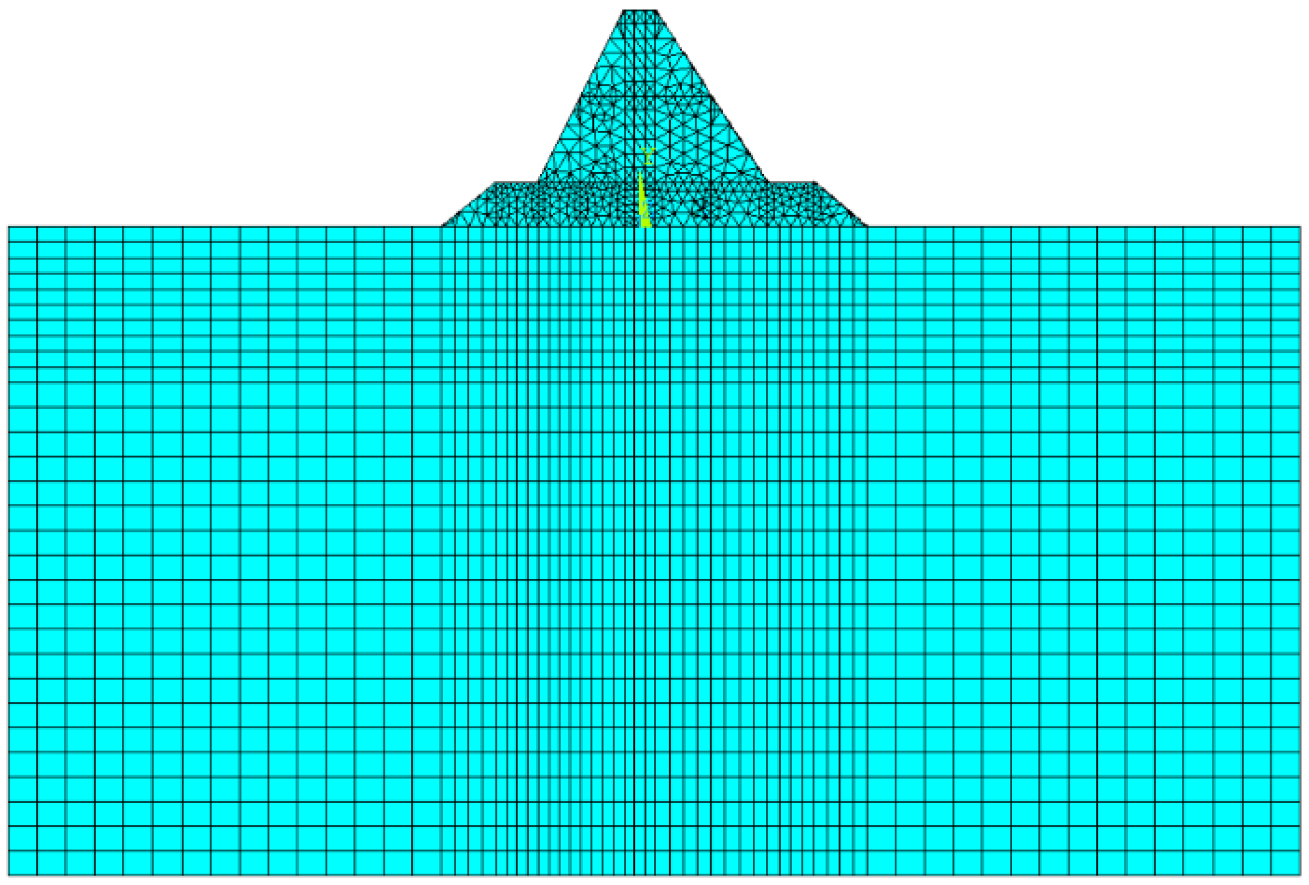
Using the direction of the river flow as the positive direction of the X-axis, the upward direction perpendicular to the river flow as the positive direction of the Y-axis, and the outward direction perpendicular to the paper surface as the positive direction of the Z-axis, ANSYS is used to establish a finite element model of the CSG dam upon overburden. The specific dimensions are shown in Figure 2. The model takes a unit thickness of 1 m in the Z-axis direction, and full constraints are added to the lower boundary of the model. We apply normal constraints to the two interfaces perpendicular to the X-axis on the dam foundation, and also apply normal constraints on the two cross-sections perpendicular to the Z-axis, forming a three-dimensional model of the dam with unit length. The model adopts mapping mesh division, and 4882 mesh elements are divided, with a total of 5002 nodes. The diagram is shown in Figure 3.
2.2. Project Overview and Establishment of Finite Element Model
CSG materials have obvious nonlinear characteristics. Currently, the Duncan–Chang hyperbolic model is widely used in the stress–strain analysis of CSG materials in engineering [17]. This model has a mature theory, rich practical experience, and is simple to apply in finite element software. The material of the engineering dam uses the Duncan–Chang model modified by the virtual rigid spring method.
2.2.1. Duncan–Chang Classical Model
In this model, the tangent modulus of elasticity is represented by , and the calculation formula is
where is the cohesion of the material; is the internal friction angle of the material; is the failure ratio; is the standard atmospheric pressure; is the base number of elastic modulus; is the index of elastic modulus. and are measured by the test.
The expression for the tangent Poisson ratio in the model is
where is the base number of tangent Poisson’s ratio; is a parameter reflecting the decrease in the initial tangent Poisson’s ratio with the decrease in the minor principal stress; is the reciprocal of the small asymptotic value on the curve of relationship between lateral strain and axial strain.
2.2.2. Principle of Virtual Rigid Spring Method
The virtual rigid spring method is used to correct the softening of the deviatoric stress in CSG materials after reaching its peak value. At this stage, the deviatoric stress () decreases as the axial strain increases, and the tangent elastic modulus is negative at this time. Therefore, the classical hyperbolic model cannot be directly used [18].
Curve 1 in Figure 4a is the actual stress–strain curve of the material, and the stress–strain relationship at this time does not satisfy the classical hyperbolic model. Adding a virtual spring at the appropriate position on the curve, as shown in Figure 4b, the stress–strain relationship of this virtual spring is shown as curve 2 in Figure 4a. The stress–strain curve after adding the virtual spring becomes hyperbolic, and the stress softening stage disappears (as shown by curve 3 in Figure 4a). Then, the true tangent elastic modulus of CSG material is
where is the actual tangent elastic modulus of CSG material; is the elastic modulus of the virtual rigid spring, and the absolute value of the maximum negative elastic modulus of the actual stress–strain curve is taken; is the tangent modulus of the virtual model [19].
2.3. Constitutive Model of Overburden and Foundation
Cemented sand gravel dams are generally built on riverbeds rich in sand and gravel. Considering the actual situation of the project and the research needs, the constitutive model of the overburden adopts the common Mohr–Coulomb constitutive model [21]. The bedrock part is relatively hard and adopts the linear elastic model. The constitutive parameters of this instance are shown in Table 2.
2.4. Implementation of Nonlinear Computing
The CSG dam is a nonlinear dam, and in nonlinear calculations, it is necessary to use a step-loading approach [22]. In order to automatically update the elastic parameters of each unit after each load step according to the change in stress state and simplify the calculation process, it is necessary to create a macro command for the Duncan–Chang constitutive relationship [23]. The step-by-step of loads requires the restart technology. After each solution is completed, the files with the suffixes “rst”, “rxxx”, and “ldhi” in the working directory need to be deleted, and a single-point restart is used for subsequent calculations [24]. In order to achieve the above requirements, the parameterized programming design language APDL module in ANSYS is selected to carry out numerical simulation calculations for CSG dam. The flowchart is shown in Figure 5. Considering both completion and impounding periods, water pressure, uplift pressure, and sediment pressure are considered during the impounding period. At the same time, using APDL also facilitates the use of MATLAB to call the ANSYS program for batch processing operations, obtaining the amount of data required for neural network training.
After loading the self-weight of the bedrock, we use the “INISTATE, WRITE” command to store the stress state, then use the “INISTATE, READ” command to read the initial stress of the bedrock before the subsequent load step, resulting in an additional displacement which is the same size but opposite direction as the original load, so that the initial displacement field of the structure turns zero, thereby achieving geostress balance. The principle is to use the constrained load balancing method to eliminate the impact of settlement caused by self-weight of the bedrock [25].
2.5. Stress–Strain Analysis
In the early phase of the engineering design, relevant organizations used the material mechanics method to calculate the compressive stress at the junction with the dam foundation under two working conditions: completion period and impoundment period. The result shows that the maximum compressive stress in the completion period and the impoundment period is, respectively, 0.4 MPa and 0.43 MPa, both of which meet the relevant design requirements. The assumptions about materials in the mechanics of materials method are all linear elastic, which differs from the actual situation. Therefore, it is hoped to conduct finite element numerical simulation for verification. The finite element calculation results show that the maximum compressive stress at the junction of the dam body and foundation in the completion period is 0.45 MPa, located near the heel of the dam. In the impoundment period, the maximum compressive stress is 0.46 MPa, located near the toe of the dam. It is found by the finite element results that due to this dam type with two stages, the compressive stress occurs at the junction of the first and second stages, different from the dam type with single stage whose maximum compressive stress is at the junction of the dam body and foundation. The following text provides a detailed analysis of the characteristic values of the dam body.
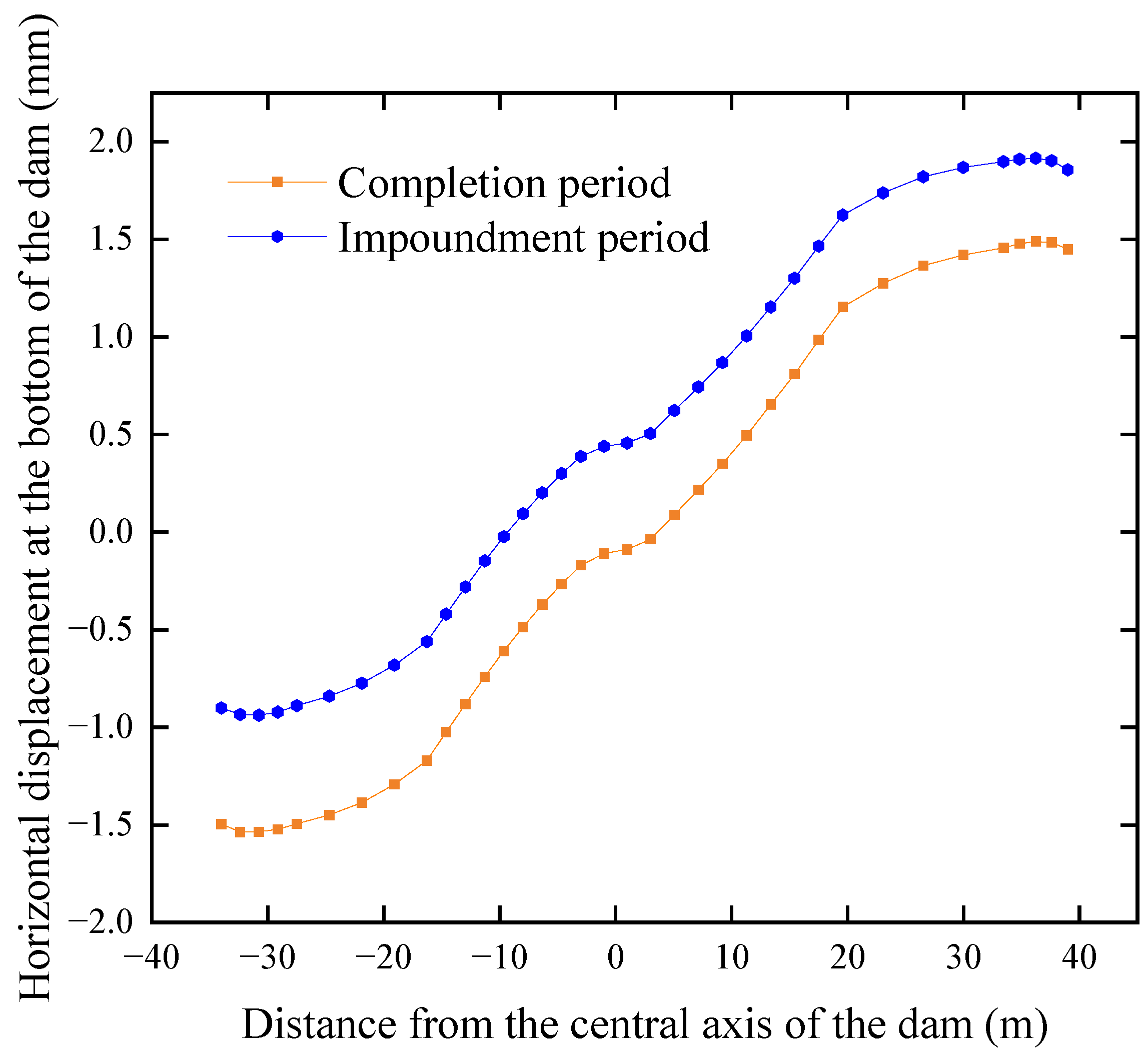
The results of the completion period and the impounding period are selected for comparison. Figure 6 shows the horizontal displacement at the bottom of the dam body. The value of the horizontal axis represents the distance between the nodes at the bottom of the dam body and the centerline of the dam body. The positive direction of the horizontal axis is along the river direction, and the negative direction of the horizontal axis is against the river direction. The negative vertical axis represents displacement against the river direction, while the positive vertical axis represents displacement along the river direction. It can be seen that, with the centerline of the dam body as the boundary, the bottom of the dam body in the upstream part deviates upstream, and the closer to the centerline, the smaller the displacement value. The bottom of the dam body in the downstream part deviates downstream, and also the closer to the centerline, the smaller the displacement value. This is due to the symmetry of the cemented gravel dam body. During the impounding period, the displacement of the dam body bottom generally deviates downstream by about 0.5 mm, with larger displacement around the upstream dam heel and downstream dam toe, with the maximum displacement at the upstream dam heel position, and smaller displacement on both sides of the centerline.
The characteristic values and positions of the dam body in the completion and impounding period are shown in Table 3. Maximum displacement in the X-direction in both completion and impounding periods occurs at the downstream toe of the first stage of the dam body, and the direction of displacement is along the river direction. Due to the influence of upstream water pressure, the maximum displacement in the X-direction in the impounding period is greater than that in the completion period. The maximum settlement in the Y-direction also increases under the influence of water pressure during the impounding period, but due to the influence of uplift pressure, some of the settlement is offset, so the final value of settlement does not change significantly, but the position of the extreme value is shifted upstream relative to the completion period. The maximum compressive stress in both completion and impounding periods occurs at the upstream dam heel where the first and second stages of the dam body meet, indicating that this is a weak point of this type of the dam with two stages. Although the compressive stress of 2.451 MPa is less than the compressive strength (6 MPa) of the dam material, it is still hoped that through optimization of the structure, the compressive stress at this location can be better balanced. The maximum tensile stress at the bottom of the dam body is due to the dam body extruding the overburden, resulting in extreme values at the contact surface.
2.6. Analysis of Factors Affecting Characteristics
There have been many studies on the influence of dam material properties on the stress–strain characteristics of CSG dam. However, there are relatively few studies on the influence of geometric properties such as dimensions and shape of dam, as well as material properties of the overburden, on the characteristics of stress and displacement of CSG dams. A sensitivity analysis of the input parameters can provide insight into the numerical simulation model’s robustness and the significance of various parameters. The change in slope coefficient will have a significant impact on the distribution of internal stress in the dam, and the change in the characteristics of the overburden will cause changes in the deformation of the dam body above it, leading to changes in stress. Meanwhile, based on the requirements of optimizing the design of the dam’s section in the following text, this paper selects six parameters: the upstream and downstream slope coefficients (, is the slope ratio, is the slope coefficient) of the first and second stages of the dam body, the elastic modulus of the overburden, and the Poisson’s ratio of the overburden. The study focuses on the influence of these six factors on two characteristic values: the maximum settlement and the maximum compressive stress of the dam body during the impounding period. The first four factors are geometric parameters of the dam body, while the last two factors are material properties of the overburden. To make the tables and figures more concise, abbreviations are used to refer to various parameters. Among them, the downstream slope coefficient of the second stage of the dam is represented by , the upstream slope coefficient of the second stage of the dam body is represented by , the downstream slope coefficient of the first stage of the dam body is represented by , and the upstream slope coefficient of the first stage of the dam body is represented by , as shown in Figure 7. refers to the elastic modulus of the overburden, refers to the Poisson’s ratio of the overburden, refers to the maximum settlement of the dam body, and refers to the maximum compressive stress of the dam body. The influencing factors and working conditions of this experiment are shown in Table 4.
As shown in Figure 8a, the maximum settlement of the dam body increases with the increase in the four slope coefficients, that is, whether it is the first or second stages of the dam body, upstream or downstream, the maximum settlement of the dam body increases with the decrease in their slope. The impact resulting from changes in and is slightly smaller than that of changes in and , because the height of the first stage of the dam is smaller than that of the second stage. As shown in Figure 8b, the maximum settlement of the dam body decreases with the increase in the . When the increases from 700 MPa to 1200 MPa, due to the increased rigidity of the overburden, the settlement of the overburden increases, and the maximum settlement of the dam body decreases due to its influence. When the increases from 1200 MPa to 1700 MPa, the decrease in maximum settlement of the dam body slows down. When increases, the lateral deformation ability of the overburden increases, the horizontal displacement increases, and the vertical displacement decreases, which also leads to a decrease in the settlement of the overburden, thus reducing the maximum settlement of the dam body. This law is more inclined to rigid dams rather than rockfill dams, which is due to the characteristics of the type of the CSG dam with dual-stage and the long maintenance time of CSG materials of the dam. As shown in Figure 9a, it can be seen that the maximum compressive stress of the dam body decreases with the increase in , and the change amplitude is small; when , , and increase, the maximum compressive stress of the dam body also increases, among which the change is particularly evident when the and increase from 0.55 to 0.70, because the maximum compressive stress just appears at the junction between the first and second stages of the dam body, so when the upstream slope coefficient of the second stage changes, it will directly change the stress condition near the maximum compressive stress value point. As shown in Figure 9b, it can be seen that changes in and also have a significant impact on the compressive stress of the dam body. When rigidity and lateral deformation ability of the overburden increase, maximum compressive stress decreases, and stress state distribution becomes more uniform.
2.7. Grey Relational Grade Analysis
To more clearly demonstrate the influence of the geometric parameters of the dam body and the characteristics of the overburden material on the maximum settlement and maximum compressive stress of the CSG dam, and to consider the amount of data required for neural network training in the following text, a numerical simulation experiment with six factors and three levels (a total of 36 = 729 groups) was conducted. In order to maximize the calculation efficiency, a nonrepetitive permutation combination method is adopted for the combination of parameters, using MATLAB software to call ANSYS for multistep loading, and implementing secondary development of finite element post-processing and batch data processing in MATLAB. Based on the previous analysis, it can be seen that the maximum settlement and maximum compressive stress of the dam are affected by the upstream and downstream slope coefficients of the first and second stages of the dam body, as well as the elastic modulus and Poisson’s ratio of the overburden. Grey relational grade is introduced to analyze and obtain the correlation level of each influencing factor. This method uses correlation to show the relationship between various factors. If the changing trends between the two factors are similar, it indicates that the correlation between the two is relatively high, otherwise the correlation is small [26]. The formula for grey correlation analysis using MATLAB software for maximum settlement of the dam is as follows:
where is the difference coefficient matrix; is column matrix, representing the sequence of maximum settlements here; is -th element of the -th influencing factor; is the correlation coefficient matrix; is the minimum value in the ; is the maximum value in the , is the element in the -th row and -th column of the ; is the resolution coefficient, with a value range of 0~1, 0.5 is taken [27].
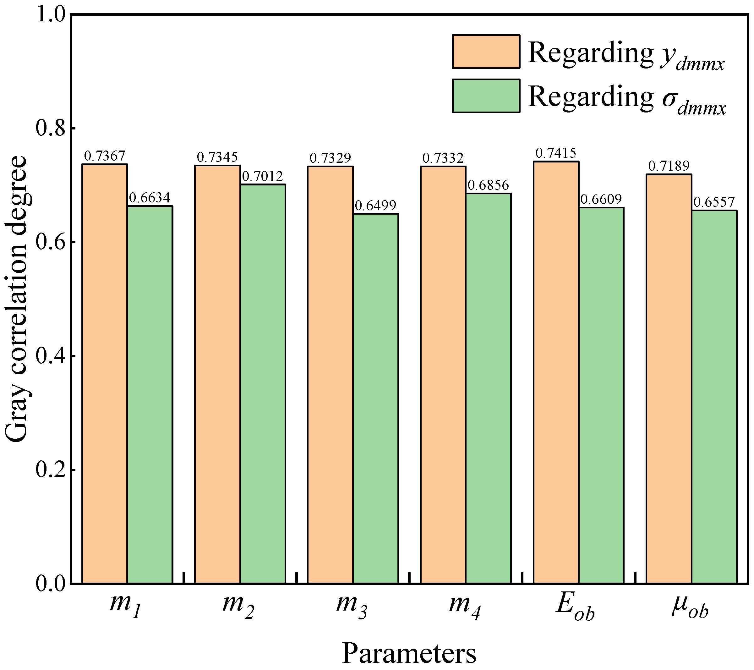
is obtained by normalizing all input variables, resulting in a matrix with 729 rows and 6 columns. Each element normalized in corresponds to the maximum settlement of the dam body of each input variables (i.e., variables normalized for each row in ) in sequence. In , each column from left to right corresponds to , , , , , and , respectively. After conducting a grey relation analysis between the influencing factors and the maximum settlement of the dam according to Equation (6), correlation coefficient matrix is calculated. By summing up the elements in each column and taking the average value, the relation degree between the corresponding influencing factors and the maximum settlement values of the dam body is obtained. Finally, it is obtained that the grey correlation matrix is R = [0.7367 0.7345 0.7329 0.7332 0.7415 0.7189]. It can be seen that there is a high correlation between the influencing factors selected for research in this paper and the maximum settlement of the dam body. The settlement extremum is most sensitive to changes in the elastic modulus of the overburden, followed by the downstream slope coefficient of the second stage of the dam body, and shows the least sensitivity to the downstream slope coefficient of the first stage of the dam body.
Similarly, the grey correlation matrix between the influencing factors and the extreme compressive stress of the dam body can be obtained as R′ = [0.6634 0.7012 0.6499 0.6856 0.6609 0.6557]. It can be seen that all six selected parameters have a high correlation with maximum compressive stress of the dam body. Among them, the upstream slope coefficient of the first stage of the dam body has the greatest impact on the maximum compressive stress, which is highly consistent with the analysis in the previous text. Figure 10 shows the correlation between the selected parameters for numerical simulation and the extreme values of dam settlement and compressive stress.
3. Neural Network Model
3.1. Data Normalization
Since , , , , , and in this numerical simulation are all highly related to the dam’s maximum settlement and compressive stress, these six variables are all determined to be selected as the input layer for this neural network model. Due to the significant differences in units and orders of magnitude between the six input parameters (four slope coefficients, elastic modulus of the overburden, and Poisson’s ratio of the overburden) and the two output parameters (maximum settlement and compressive stress of the dam body), in order to improve the accuracy and precision of training neural networks, it is necessary to normalize all data [28]. We normalize the data to the range of [0, 1] using the following formula:
where x represents the raw data, and y represents the normalized data.
3.2. BP Neural Network
A BP (backpropagation) neural network is a multilayer feedforward neural network trained on error backpropagation. The learning process can be summarized as follows: forward propagation of signals, backward propagation of errors, updating of weights and thresholds [29]. The core principle of this algorithm is to train the model on the backpropagation error to minimize error and attain high accuracy [30].
The number of input units in the neural network is 6, and the number of output units is 2. According to Kolmogorov’s theorem, when the number of hidden layers is 1, a BP neural network can approximate any nonlinear continuous function with arbitrary accuracy [31]. In this BP neural network model, when the number of hidden layers is 1, it can exhibit excellent data regression performance, so it is determined that the number of hidden layers is 1. However, the number of nodes under a single hidden layer has a significant impact on data regression. Too few nodes in the hidden layer may lead to underfitting due to poor learning ability, while too many nodes may cause overfitting due to strong learning ability. In order to prevent overfitting while ensuring the regression performance of the data, it is necessary to use a combination of empirical formulas and conduct experiments of cyclic code to determine the value of the number of nodes. According to empirical formula 9, the range of the number of hidden layer nodes is 3~12. Through continuous trial and error, combined with empirical formulas, the parameters of the BP network model are set as follows: the activation function between the input layer and the hidden layer is tansig, the connection function between the hidden layer and the output layer is purelin, the training function is trainlm, the network learning rate is 0.01, the additional momentum factor is 0.9, the epoch is 1200, and the target error is 1e-04. The number of hidden layer nodes is determined by using cyclic code to select the minimum mean square error. Figure 11 shows the mean square error of the BP neural network under different node numbers. As can be seen, when the number of nodes is set to 3, the MSE is relatively large. As the number of nodes increases, the MSE gradually decreases. When the number of nodes is set to 10, the MSE tends to flatten, and when it reaches 12, the MSE is the smallest. Therefore, based on the result and the range specified by the empirical formula, the number of nodes is set to 12. The neural network modeling scheme is shown in Figure 12.
where is the number of hidden layer nodes; is the number of input layers; is the number of output layers, and is an integer ().
3.3. Evaluation Indicators of Predictive Performance
The root mean square error (RMSE), mean absolute percentage error (MAPE), and coefficient of determination (R2) are three commonly used indicators to evaluate the effectiveness of a neural network. RMSE is a unit quantity that clearly shows how much the predicted value deviates from the true value, and MAPE is a percentage quantity without unit dimension, which can visually show the degree of deviation from the predicted value. A higher determination coefficient signifies better performance of the prediction model [32]. R2 can reflect the degree of regression of data in neural network prediction models. The formula expressions for RMSE, MAPE and R2 are as follows:
where is the actual value calculated through numerical simulation, is the predicted value of the neural network model, is the number of predicted points, and is the mean of the actual value calculated through numerical simulation.
3.4. Regression Analysis of BP Neural Network Model Data
After preprocessing 729 sets of sample data, they were randomly divided into training and testing sets, with the training set accounting for 7/10 and the testing set accounting for 3/10. There were 510 groups of data in the training set and 219 groups of data in the testing set. The sample data were imported into the BP neural network for data regression analysis.
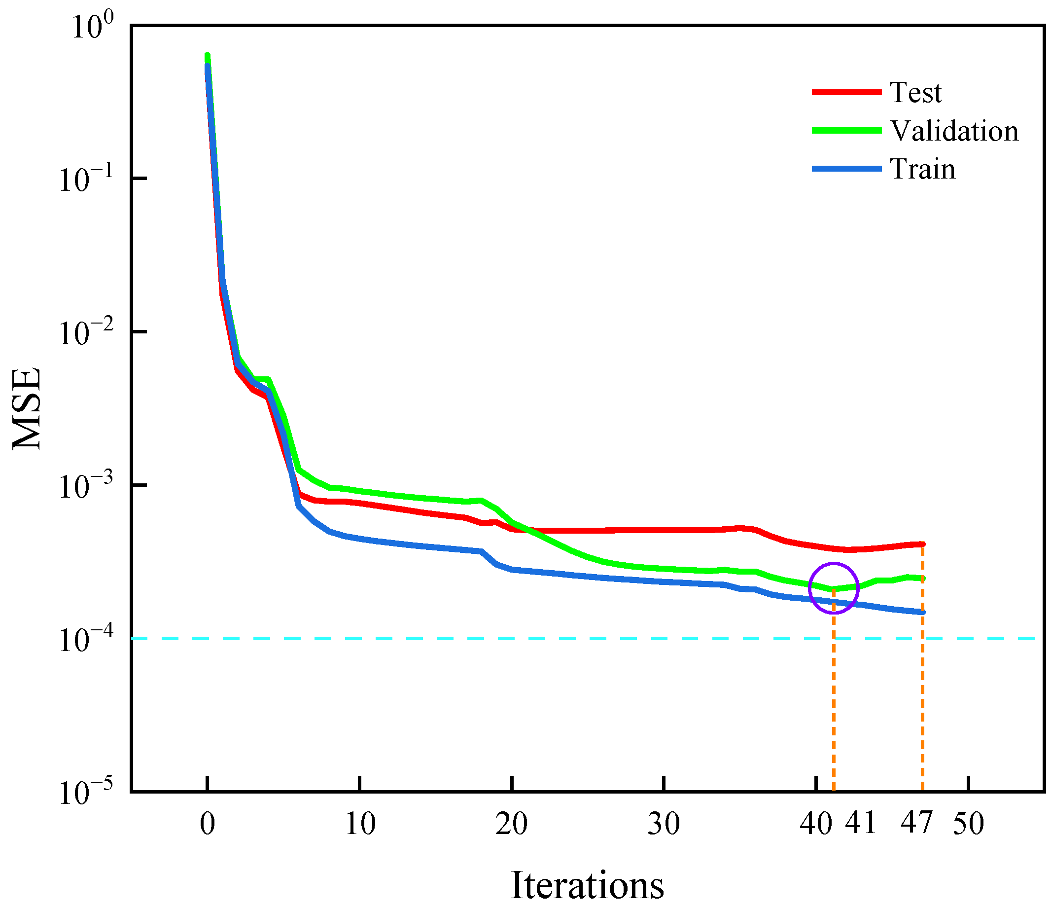
The predicted values of the BP neural network are nonlinear function output values, so the prediction accuracy of the BP neural network is of great significance for finding the optimal value in the following text. The BP neural network completed 6 rounds of cross-validation in the 47th iteration, and the optimal validation error occurred in the 41st iteration, which is 2.08 × 10⁻⁴, as shown in Figure 13.
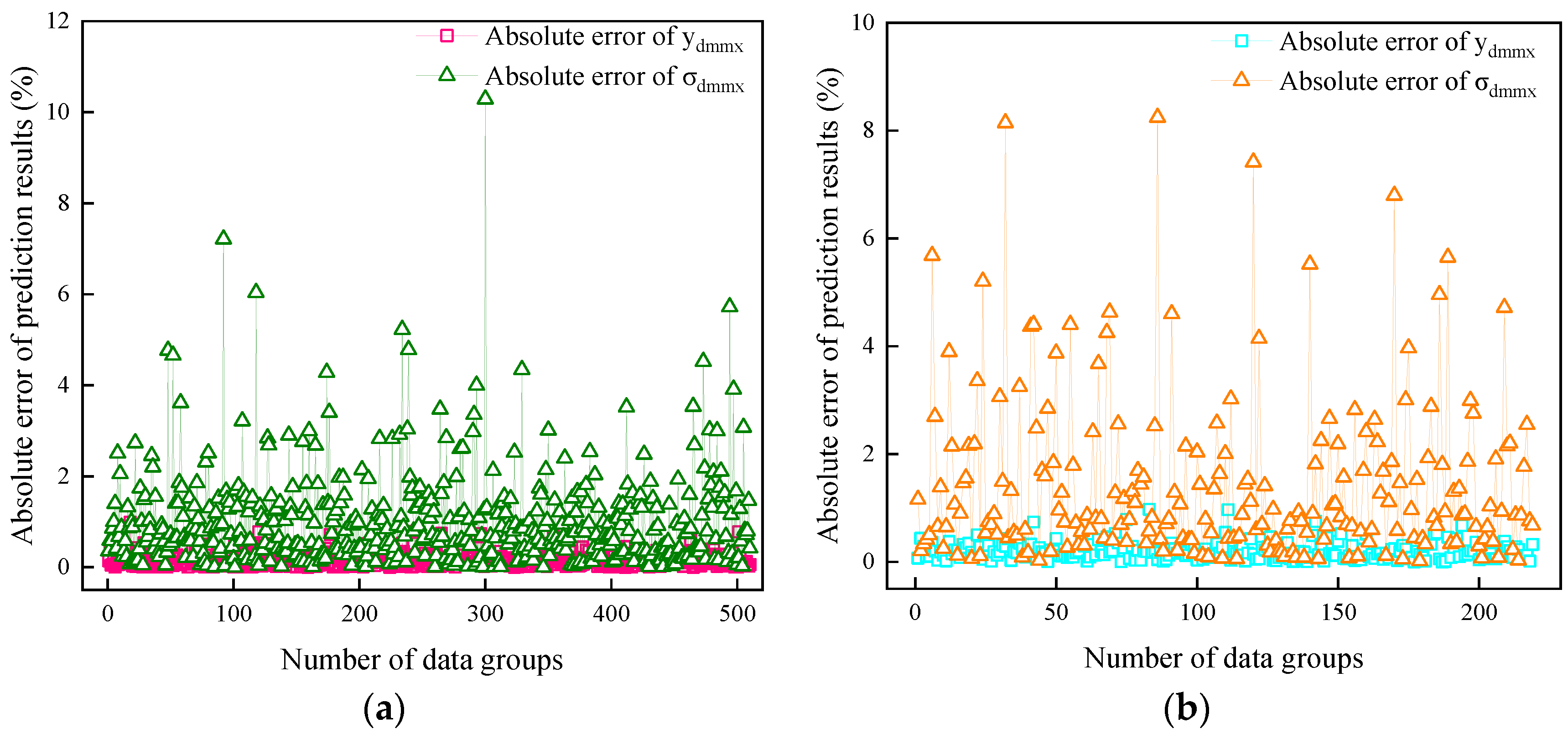
To verify the reliability of the neural network, data of the training set and testing set are used to validate the neural network model. The error bands between the neural network prediction results and numerical simulation results are shown in Figure 14, indicating that the neural network has good fitting effects on both the maximum settlement and the maximum compressive stress of the dam body. From Figure 15a, it can be seen that the absolute error in predicting the maximum settlement of the dam body in the training set is controlled within 1%; the absolute error of the maximum compressive stress is only one that exceeds 10%, while the rest is controlled within 8%, but most do not exceed 2.5%. From Figure 15b, it can be seen that the absolute error in predicting the maximum settlement of the dam body is all controlled within 1%. The maximum absolute error has only a few that exceed 8%, but the maximum does not exceed 8.5%, and most are within 3%. From this, it can be analyzed that there was no phenomenon of overfitting in the prediction of the extreme values of characteristics of the dam. That is to say, the phenomenon of good prediction performance in the training set, but poor testing performance in the prediction set, did not occur.
According to the statistical results, as shown in Table 5, in the prediction of the maximum settlement of the dam body, the RMSE, MAPE, and R2 of the training set are 0.0095 cm, 0.18%, and 0.9997, respectively, while the RMSE, MAPE, and R2 of the test set are 0.0109 cm, 0.21%, and 0.9996, respectively, indicating excellent evaluation indicators. In the prediction of the maximum compressive stress of the dam body, the RMSE, MAPE, and R2 of the training set are 0.0239 MPa, 1.03%, and 0.9931, respectively, while the RMSE, MAPE, and R2 of the test set are 0.0335 MPa, 1.43%, and 0.9871, respectively. The evaluation indicators are slightly inferior to the results of the prediction of the maximum settlement, but still excellent. The evaluation indicators of the training set and the prediction set are highly consistent, and there is no situation where the training set performs well but the test set performs poorly, once again confirming that the prediction has not fallen into local optima.
4. Optimization Design
Long-term factors of creep, shrinkage, ageing, and corrosion in civil engineering structures are often overlooked but are critical [33], so the maximum compressive stress value of the dam body is not only one of the indicators to determine whether the material will be damaged, but also one of the references to measure the uniformity of the stress distribution of the dam body and judge the rationality of the shape of the dam. Deformation can effectively reflect the structural state of dams [34], and the excessive settlement of the dam body can cause structural deformation and stress concentration; excessive settlement can lead to structural deformation, which may cause water seepage, and, thus, affect the stability and operation effect of the dam body. Therefore, based on engineering needs and safety considerations, it is hoped that the geometric dimensions of the dam body can be optimized through structural design while ensuring that the extreme values of compressive stress and settlement of the dam body are not greater than the initial dam size, so as to reduce the consumption of dam materials and achieve economic benefits.
4.1. Process of Optimization
Using the parameterization design concept, the characteristic parameters of the model are abstracted based on its geometric structure. The following four design variables are adopted: M1 is the downstream slope coefficient of the second stage of the dam body, M2 is the upstream slope coefficient of second stage of the dam body, M3 is the downstream slope coefficient of the first stage of the dam body, and M4 is the upstream slope coefficient of the first stage of the dam body, as shown in Figure 16. Because the width of the dam body is uniform in the direction perpendicular to the river, the volume of the dam body with a width of one meter is selected as the objective function. When the objective function reaches its minimum, it means that the volume of the dam body is minimized, and this situation is considered as the minimum material consumption in this paper.
According to relevant design specifications [35,36,37], it can be seen that the design requirements for this dam body are as follows: the range of upstream and downstream slope ratio of the first stage of the dam is 1:1.5~1:0.6; the range of upstream slope ratio of the second stage of the dam is 1:0.4~1:0.7; the range of downstream slope ratio of the second stage of the dam is 1:0.5~1:0.8; the vertical stress of the dam heel does not exhibit tensile stress; there is no tensile stress on the upstream surface of the dam body; the maximum compressive stress of the dam body does not exceed the maximum allowable compressive stress of the material; the stress ratio between the heel and toe of the dam does not exceed the allowable value of 1.5. In the early phase of engineering design, the material mechanics method was already used to conduct reliability calculations on the dam body, which meets the requirements of relevant specifications. This paper uses the finite element method for verification and obtains the following results: the vertical stress at the heel position of the dam body is −0.23 MPa, which is the compressive stress; the maximum stress in the upstream of the dam body is −0.01 MPa, which means it is all under compression stress conditions; the maximum value of compressive stress of the dam body is 2.41 MPa, which is less than the compressive strength of the material by 6 MPa; the compressive stress at the heel of the dam is 0.39 MPa; the compressive stress at the toe of the dam is 0.33 MPa; the stress ratio between the heel and toe of the dam is 1.18, meeting the requirements of the specification within the range of 1.5. All review results are safe. Therefore, when conducting optimization, only the geometric conditions of the dam body specified in the specifications are included in the constraint conditions. After finding the optimal solution, the parameters of the found optimal solution are inputted into ANSYS for numerical simulation to see whether the other conditions required by the relevant specifications are met. If not, the previous optimal solution is attempted, and so on. This can greatly improve optimization efficiency.
4.2. Objective Function and Constraints
The purpose of optimizing design is to ensure that the characteristic values of stress and displacement of the dam body are not weaker than those of the initial dam, and the material consumption turn is minimized, thereby achieving maximum economic benefits and saving expenses in the engineering budget. The objective function is denoted as
where is the cross-sectional area of the dam body.
In order to meet the requirements of the specifications, the range of slope requirements in the specifications is converted into the constraint of slope coefficients; the constraint conditions are as follows.
Geometric constraints:
0.5 ≤ M1 ≤ 0.8
0.4 ≤ M2 ≤ 0.7
0.6 ≤ M3 ≤ 1.5
0.6 ≤ M4 ≤ 1.5
Stress–strain constraints:
where is the maximum settlement of the dam body, predicted by neural network; is the maximum compressive stress of the dam body, predicted by neural network; is the maximum settlement of the initial dam, which is 4.190 cm; is the maximum compressive stress value of the initial dam, which is 2.41 MPa.
4.3. Implementation and Comparison of Optimization
In engineering, a commonly used optimization method is to mix finite element software with optimization tool software or other optimization functions. The principle of this method is that the optimization part transfers the design variables generated by a single exploration to the finite element software, which calculates the stress–strain results and returns them to the optimization software for judgment. The optimization software then proceeds to the next step of optimization until the optimal solution is found. Although this method solves the problems of limited algorithm types and low adaptability in traditional finite element software’s built-in optimization tools, it still does not solve the problems of slow operation and low efficiency, because each optimization requires one operation of finite element, which is the most time-consuming part of the optimization process. Therefore, the maximum number of optimization times becomes the bottleneck of traditional optimization methods. If neural networks are used to replace the role of finite element software in the optimization process, this deficiency can be compensated for. After the neural network prediction model is trained, it is equivalent to finding the mapping relationship between the design variables and the objective function and constraint conditions. Therefore, during the optimization process, finite element calculations are no longer needed.
The result of the trained BP neural network is saved to a file with the suffix “mat”, and the optimize calculation is conducted by using the global optimization tool Pattern Search in the MATLAB toolbox. The specific format for calling this optimization algorithm is as follows:
[x,fval,exit,output] = patternsearch(fun,x0,A,b,Aeq,beq,lb,ub,nonlcon,options)
Here, fun is the function name for the objective function with respect to design variables, matrix A and vector b, respectively, represent the terms at the left and right ends of the linear inequality constraint, the matrix Aeq and vector beq, respectively, represent the terms at the left and right ends of a linear equation constraint, and lb and ub represent the upper and lower limits of design variables.
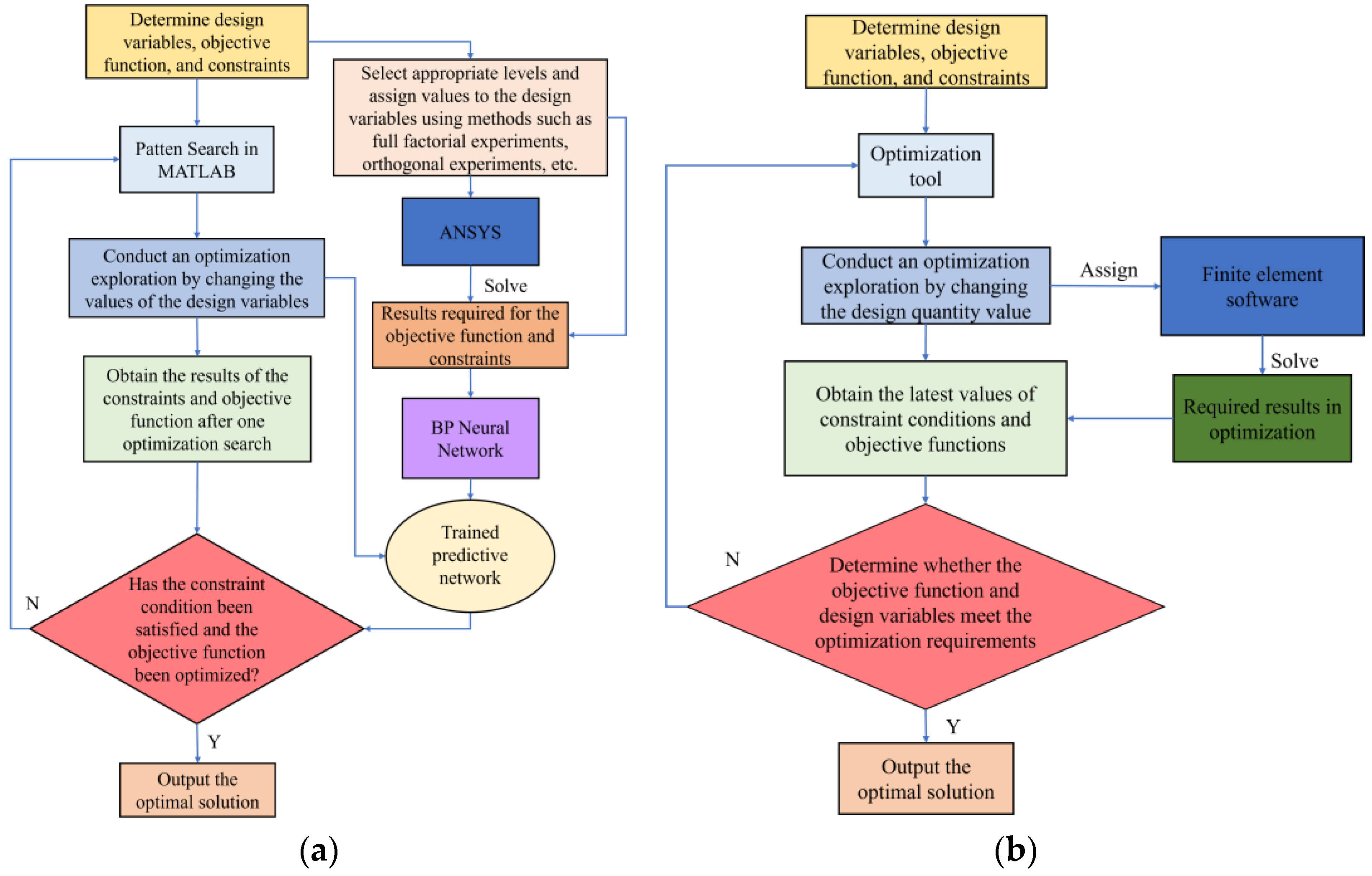
The flowchart for implementing the optimization idea is shown in Figure 17a. As a comparison, the traditional optimization method is shown in Figure 17b. It can be seen that in the traditional optimization method, the calculation results of each finite element software are not fully utilized, but only the values required for the objective function and constraints are provided. In this paper, the results of ANSYS calculation are retained and used for training the neural network, which can be fully and comprehensively utilized.
4.4. Analysis of Optimization Results
After the above optimization process, the optimal solution is obtained: [M1 M2 M3 M4] = [0.503 0.402 0.653 0.765]. In order to form a comparison, this paper also compiles the programming of the traditional optimization method. To ensure the fairness of the comparison as much as possible, the traditional optimization methods still use the Pattern Search tool in the MATLAB toolbox. However, due to the fact that each optimization in traditional optimization methods requires a finite element operation, the maximum number of optimizations in traditional optimization methods is set to 2000 to prevent excessive time of computation. The optimal solution obtained by traditional optimization methods is [0.517 0.402 0.653 0.647]. We substitute the calculation results of the two methods into ANSYS for review, and the results are shown in Table 6. In the table, represents the vertical stress at the heel position of the dam body, represents the maximum stress in the upstream of the dam body, represents the maximum value of compressive stress of the dam body, represents the compressive stress at the heel of the dam, and represents the compressive stress at the toe of the dam. As can be seen, the verification results all meet the requirements in the specifications.
Table 7 lists the characteristic values of the initial, optimized dam size by traditional method and optimized dam size by method based on BP neural network, where refers to the amount of material used per one meter thickness of the dam body. The operation of both methods is based on the X86 architecture platform, with AMD7945hx CPU, Nvidia 4060 laptop GPU, 16 GB memory, and Windows 11 operating system. The time consumption of both methods is recorded separately. When using the optimization method based on BP neural network, it takes 4 h and 17 min to obtain the 729 sets of data from ANSYS used for training the network, the training time for BP neural network is 15 s, and the time consumed by Pattern Search tool is 12 min, totaling 4 h and 30 min.
The effect diagram of section optimization based on the BP neural network optimization design method is shown in Figure 18.
4.5. Evaluation of Optimization
After the optimization of the dam body, the material consumption per unit thickness is saved by 11.83%, the maximum settlement of the dam body is reduced by 2.60%, and the maximum compressive stress of the dam body is reduced by 37.35% compared to the initial dam body, achieving an improvement in stress state and economic benefits.
The optimization method based on the BP neural network finds a better solution. Although the minimum value of the objective function is only 0.3% different from the value calculated by traditional optimization method, the time consumption is saved by 40.92% by using the optimization method based on BP neural network, greatly improving computational efficiency and saving computational resources.
In the combination of neural network prediction and optimization design methods, the prediction error after neural network training is one of the key factors affecting the optimization effect. In this paper, the prediction effect is good because the data source is calculated by finite element software. The neural network model shows high accuracy in predicting relatively regular and almost noise-free datasets, which also makes the method of accelerating structural optimization design by neural network prediction model feasible and reasonable.
5. Discussion
This paper is based on an actual engineering project of a CSG dam with two stages, designed according to some practical requirements, and it introduces a design method for implementing nonlinear calculations in ANSYS. A numerical model for the CSG dam upon overburden is established using an improved Duncan–Chang constitutive model. The effects of geometric dimensions of the dam body and characteristics of the overburden are considered. The grey relational grade between influencing factors and the dam’s maximum settlement and maximum compressive stress is discussed. Based on the results of grey correlation degree, a BP neural network model is established, and the maximum settlement and maximum compressive stress of the dam body is predicted with high accuracy. Combined with the trained prediction model, an optimization method is designed to maximize the economic benefits of the dam under the premise of improving the stress deformation state. The results of the analysis of influencing factors show that changes in the upstream and downstream slope coefficients of the dam have a significant impact on the stress and settlement of the dam. With a trained neural network model, in practical engineering, the results of maximum settlement and maximum compressive stress can be quickly obtained by inputting the slope coefficients and overburden properties into the neural network. Due to using the optimization design as the starting point in designing the network model, factors such as the height, the width, and dosage of cementitious materials of the dam are not considered into the neural network. But according to the outlook, this can be promoted. By considering the complete geometric dimensions, the material parameters of the dam body, and complete material parameters of the overburden into the neural network, a relatively more universal prediction model will be obtained, which can be directly used as a reference of site selection, dimension design, overburden treatment, and design optimization of CSG dams for more design organizations.
The advantages of the optimization method based on BP neural network are shown in detail, such as significant efficiency improvements, but it may also have some limitations. It heavily relies on the accuracy of the prediction model, which is a prerequisite. If encountering situations with poor prediction results, it is difficult, or even impossible, to obtain the optimal result. Therefore, improving the prediction accuracy of nonlinear calculations is also a worthwhile issue to study.
In future dam design and construction practices, the optimization methods based on neural network can be used to save time on finite element software calculations, and trained models can be saved for future use. More and more trained prediction models like those in this paper may appear, corresponding to various types of dams and geographical conditions. Designers can directly obtain references for site selection and structural design, or combine them with design optimization, which can improve the operational efficiency of the entire industry and greatly save social resources.
6. Conclusions
- (1)
- The upstream and downstream slope coefficients of the first and second stages of the CSG dam, as well as the elastic modulus and Poisson’s ratio of the overburden, all have a significant impact on the stress and deformation state of the dam body. In dimension parameters, the downstream slope coefficient of the second stage of the dam has the greatest impact on the maximum settlement, with a grey correlation degree of 0.7367. The influence of the elastic modulus of the overburden on the maximum settlement of the dam body is greater than its Poisson’s ratio.
- (2)
- The BP prediction model in this paper achieves an R2 of 0.9996 and an RMSE of 0.0109 cm when predicting maximum settlement, and achieves an R2 of 0.9871 and an RMSE of only 0.0335 MPa when predicting maximum compressive stress, which provides a prerequisite and accuracy guarantee for the optimization method based on a BP neural network. After inputting the slope parameters of the dam body and the material parameters of the overburden into the trained model, accurate maximum settlement and maximum compressive stress can be obtained.
- (3)
- Combining a BP neural network with the optimization algorithm can achieve efficient section optimization of the CSG dam. Through optimization, the material consumption of the dam body is saved by 11.83%, the maximum settlement of the dam body is reduced by 2.60%, and the maximum compressive stress of the dam body is reduced by 37.35% compared to the initial size. By using an optimization method based on a BP neural network, the time consumption is reduced by 40.92% compared to the traditional optimization method. The economic benefits of the dam are improved, the state of stress and deformation is improved, computational efficiency is improved, and computational resources are saved. The application of different prediction models and optimization algorithms in engineering optimization problems deserves more in-depth research in the future.
Author Contributions
Conceptualization, S.W.; methodology, S.W.; software, S.W.; validation, S.W. and H.Y.; resources, H.Y.; data curation, Z.L.; writing—original draft preparation, S.W.; writing—review and editing, S.W., H.Y. and Z.L. All authors have read and agreed to the published version of the manuscript.
Funding
This work is supported by National Natural Science Foundation of China project (No. 52279130).
Institutional Review Board Statement
Not applicable.
Informed Consent Statement
Not applicable.
Data Availability Statement
The original contributions presented in the study are included in the article, further inquiries can be directed to the corresponding author.
Conflicts of Interest
The authors declare no conflicts of interest.
Abbreviations
| Downstream slope coefficient of the second stage of dam | |
| Upstream slope coefficient of the second stage of dam | |
| Downstream slope coefficient of the first stage of dam | |
| Upstream slope coefficient of the first stage of dam | |
| Elastic modulus of overburden | |
| Poisson’s ratio of overburden | |
| Maximum settlement of dam body | |
| Maximum compressive stress of dam body | |
| BP | Backpropagation |
| RMSE | Root mean square error |
| MAPE | Mean square error |
| Coefficient of determination which can reflect the degree of regression of data |
References
- Sun, M.; Yang, S.; Tian, Q. Review on Mechanical Properties, Durability and Dam Type of CSG Material. Yellow River 2016, 38, 83–85. [Google Scholar] [CrossRef]
- Wang, C.; Xu, S. Adaptability Analysis of Subgrade Condition of Cement Sand Gravel Dam Based on the Mechanical Properties. Water Conserv. Sci. Technol. 2018, 24, 43–46. [Google Scholar]
- Kim, S.; Choi, W.; Kim, Y.; Shin, J.; Kim, B. Investigation of Compressive Strength Characteristics of Hardfill Material and Seismic Stability of Hardfill Dams. Appl. Sci. 2023, 13, 2492. [Google Scholar] [CrossRef]
- Jia, J.; Ding, L.; Wu, Y.; Zhao, C.; Zhao, L. Research and Application of Key Technologies for the Construction of Cemented Material Dam with Soft Rock. Appl. Sci. 2023, 13, 4626. [Google Scholar] [CrossRef]
- Yang, H.; Jia, J.; Zheng, C.; Feng, W.; Lu, Y. Research on the anti-skid stability of the surface layer of Shoukoubao cementitious granular material dam. In Proceedings of the 2014 Academic Annual Conference of the China Dams Association; Jia, J., Ji, J., Eds.; The Yellow River Water Conservancy Press: Zhengzhou, China, 2014; pp. 567–574. [Google Scholar]
- Wu, M.; Du, B.; Yao, Y.; He, X. An experimental study on stress-strain behavior and constitutive model of hardfill material. Sci. China Phys. Mech. 2011, 54, 2015–2024. [Google Scholar] [CrossRef]
- Yang, S.; Chai, Q.; Sun, M. Nonlinear Finite Element Analysis of Stress and Displacement of CSG Dam. Yellow River 2016, 38, 89–91. [Google Scholar] [CrossRef]
- Guo, X.; Du, J.; Zhao, Q.; Cai, X. Creep Test of CSG and Long-Term Deformation Prediction of CSG Dams. Yellow River 2019, 41, 149–154. [Google Scholar] [CrossRef]
- Cao, S.; Pan, X.; Gao, Y. Neural network ensemble-based parameter sensitivity analysis in civil engineering systems. Neural Comput. Appl. 2017, 28, 1583–1590. [Google Scholar] [CrossRef]
- Sun, M.; Cheng, Y.; Ma, X.; Xia, Z.; Zhou, Q.; Zhu, Q.; Xue, X. Prediction of Critical Parameters of Reprocessing Non-uniform Conditions Based on Improved BP Neural-network. Nucl. Power Eng. 2023, 44, 16–22. [Google Scholar] [CrossRef]
- Yu, J.; Jin, A.; Pan, J.; Wang, J.; Zhang, C. GA-BP artificial neural networks for predicting the seismic response of arch dams. J Tsinghua Univ. Sci. Technol. 2022, 62, 1321–1329. [Google Scholar] [CrossRef]
- Zhang, M.; Huang, J.; Wang, Y. Finite element analysis and neural-network prediction of deformation of underground pipelines affected by excavation. Chin. J. Geotech. Eng. 2006, 28, 1350–1354. [Google Scholar] [CrossRef]
- Bai, F.; Shi, W.; Bao, Z.; Xing, C. Optimization design of flat steel gates based on BP neural network and genetic algorithm. Sichuan Water Resour. 2023, 44, 42–47. [Google Scholar]
- Chen, S.; Liu, Y.; Jing, G.; Chen, G.; Peng, Q. Optimization Design of the Interference Connection Structure for Turbocharger Turbine Rotors Based on Back Propagation. Chin. Intern. Combust. Engine Eng. 2024, 45, 10–17. [Google Scholar] [CrossRef]
- Lu, H.; Zhang, J.; Lv, C.; Pan, K.; Li, Z. Optimization Design of Electromagnetic Drive Structure for Shaftless. Sci. Technol. Eng. 2024, 24, 3236–3242. [Google Scholar] [CrossRef]
- Ding, Z.; Xu, L.; Wang, X. Design method of 100-meter cemented sand and gravel dams based on multivariate optimization. J. Hydroelectr. Eng. 2023, 42, 119–131. [Google Scholar]
- Sun, M.; Wu, P.; Yang, S.; Chai, Q. Experimental Study on Constitutive Model of CSG. Yellow River 2015, 37, 126–128+131. [Google Scholar] [CrossRef]
- Sun, M.; Yang, S.; Zhang, J. Study on constitutive model for over lean cemented material. Adv. Sci. Technol. Water Resour. 2007, 27, 35–37. [Google Scholar]
- Tian, Q.; Yang, S.; Chai, Q.; Sun, M. Finite Element Analysis of Shoukoubao Dam Based on the Virtual Rigid Spring Method. J. North China Univ. Water Resour. Electr. Power 2015, 36, 30–33. [Google Scholar] [CrossRef]
- Sun, M.; Yang, S.; Chai, Q. Basic Research of Cement-sand-gravel Dam. J. North China Univ. Water Resour. Electr. Power 2014, 35, 43–46. [Google Scholar] [CrossRef]
- Shen, D.; Cai, X. Stress-strain characteristics and influencing factors of cemented sand and gravel (CSG) dam upon overburden. Water Resour. Hydropower Eng. 2019, 50, 80–86. [Google Scholar] [CrossRef]
- Kubota, S.; Kawai, Y.; Kadotani, R. Accuracy validation of point clouds of UAV photogrammetry and its application for river management. Int. Arch. Photogramm. Remote Sens. Spat. Inf. Sci. 2017, 42, 195–199. [Google Scholar] [CrossRef]
- Wu, C.; Zhang, Y.; Xu, X. Application research of APDL secondary development in nonlinear analysis of earth rock dams. Disaster Control Eng. 2010, 1, 6–10. [Google Scholar]
- Liu, Z.; Miao, L. Finite element nonlinear analysis for rockfill dam with concrete lab based on APDL. J. Northwest Hydroelectr. Power 2004, 20, 17–20. [Google Scholar]
- Wang, T.; Xu, Q. Finite Element Analysis of Rock-filled Dams Based on Duncan-Chang Model. China Rural Water Hydropower 2016, 1, 151–155. [Google Scholar]
- Ni, X.; Wang, C.; Tang, D.; Lu, J.; Wang, X.; Chen, W. Early-warning and inducement analysis of super-large deformation of deep foundation pit on soft soil. J. Cent. South Univ. 2022, 53, 2245–2254. [Google Scholar] [CrossRef]
- Yuan, Z.; Gao, L.; Chen, H.; Song, S. Study on Settlement of Self-Compacting Solidified Soil in Foundation Pit Backfilling Based on GA-BP Neural Network Model. Buildings 2023, 13, 2014. [Google Scholar] [CrossRef]
- Zhang, X.; Xu, N.; Dai, W.; Zhu, G.; Wen, J. Turbofan Engine Health Prediction Model Based on ESO-BP Neural Network. Appl. Sci. 2024, 14, 1996. [Google Scholar] [CrossRef]
- Cui, F.; Wang, H.; Shu, Z. Prediction of aerodynamic pressure amplitude in tunnel based on PSO-BP neural network. J. Cent. South Univ. 2023, 54, 3752–3761. [Google Scholar] [CrossRef]
- Pei, J.; Liu, L.; Wang, X.; Ling, Y. Derivation of Creep Parameters for Surrounding Rock through Creep Tests and Deformation Monitoring Data: Assessing Tunnel Lining Safety. Appl. Sci. 2024, 14, 2090. [Google Scholar] [CrossRef]
- Zhang, W.; Zhang, Z.; Gong, X.; Wang, X. AirFlow Angle Estimation Method for Large Passenger Aircraft Based on GA-BP Neural Network. Comput. Simulation. 2024, 41, 53–57. [Google Scholar]
- Chai, H.; Xu, H.; Hu, J.; Geng, S.; Guan, P.; Ding, Y.; Zhao, Y.; Xu, M.; Chen, L. Application of a Variable Weight Time Function Combined Model in Surface Subsidence Prediction in Goaf Area: A Case Study in China. Appl. Sci. 2024, 14, 1748. [Google Scholar] [CrossRef]
- Harapin, A.; Jurišić, M.; Bebek, N.; Sunara, M. Long-Term Effects in Structures: Background and Recent Developments. Appl. Sci. 2024, 14, 2352. [Google Scholar] [CrossRef]
- Chen, Z.; Liu, X. Multi-Point Deformation Prediction Model for Concrete Dams Based on Spatial Feature Vector. Appl. Sci. 2023, 13, 11212. [Google Scholar] [CrossRef]
- SL678-2014; Technical Guideline for Cemented Granular Material Dams. China Water & Power Press: Beijing, China, 2014.
- SL319-2018; Design Specification for Concrete Gravity Dams. China Water & Power Press: Beijing, China, 2018.
- SL265-2016; Design Specifications for Sluices. China Water & Power Press: Beijing, China, 2016.
Figure 1.
Roadmap of the study’s flow.
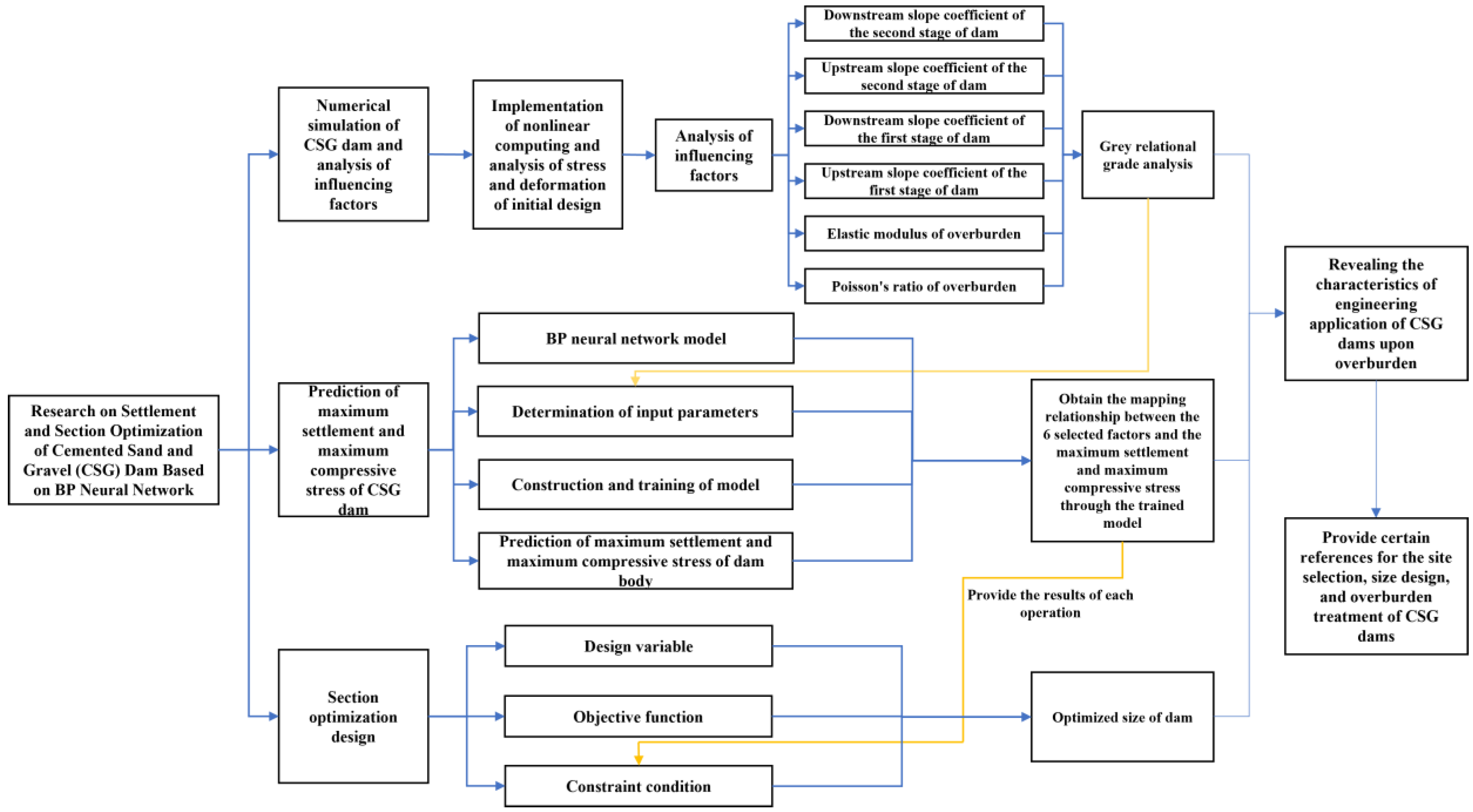
Figure 2.
Section of dam (unit: m).
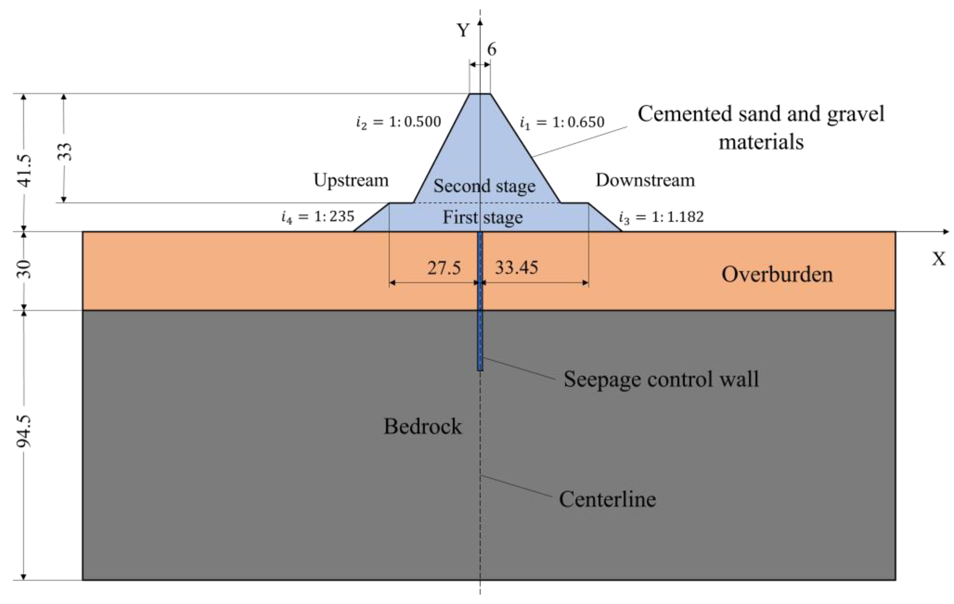
Figure 3.
Diagram of finite element mesh.

Figure 4.
Schematic diagram of virtual rigid spring method. (a) Three types of stress–strain curves; (b) virtual addition of rigid springs.
Figure 4.
Schematic diagram of virtual rigid spring method. (a) Three types of stress–strain curves; (b) virtual addition of rigid springs.
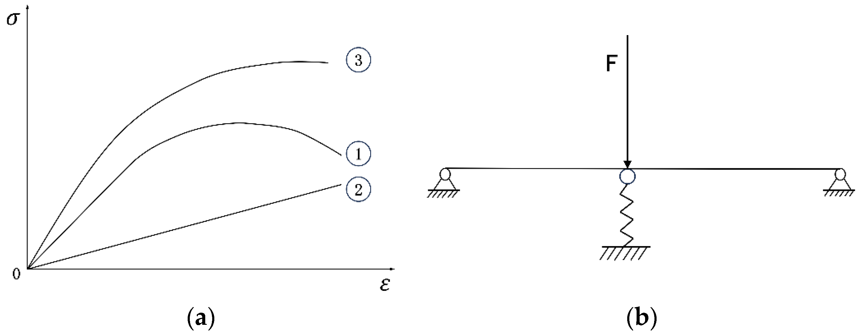
Figure 5.
ANSYS calculation process.
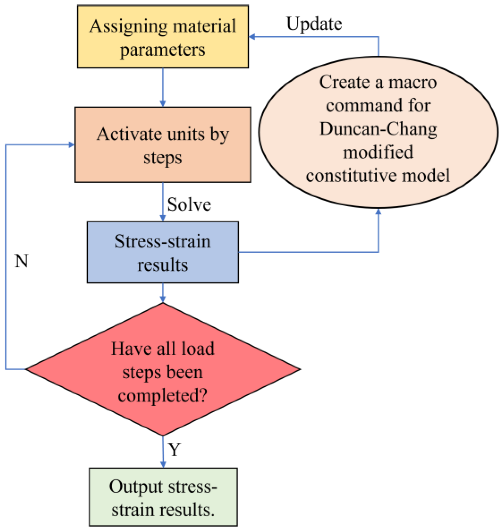
Figure 6.
Horizontal displacement at the bottom of the dam.

Figure 7.
Parameter diagram.
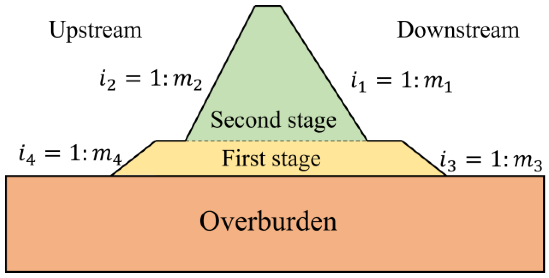
Figure 8.
Factors affecting maximum settlement. (a) Factors of geometric dimensions; (b) factors of performance of overburden.
Figure 8.
Factors affecting maximum settlement. (a) Factors of geometric dimensions; (b) factors of performance of overburden.
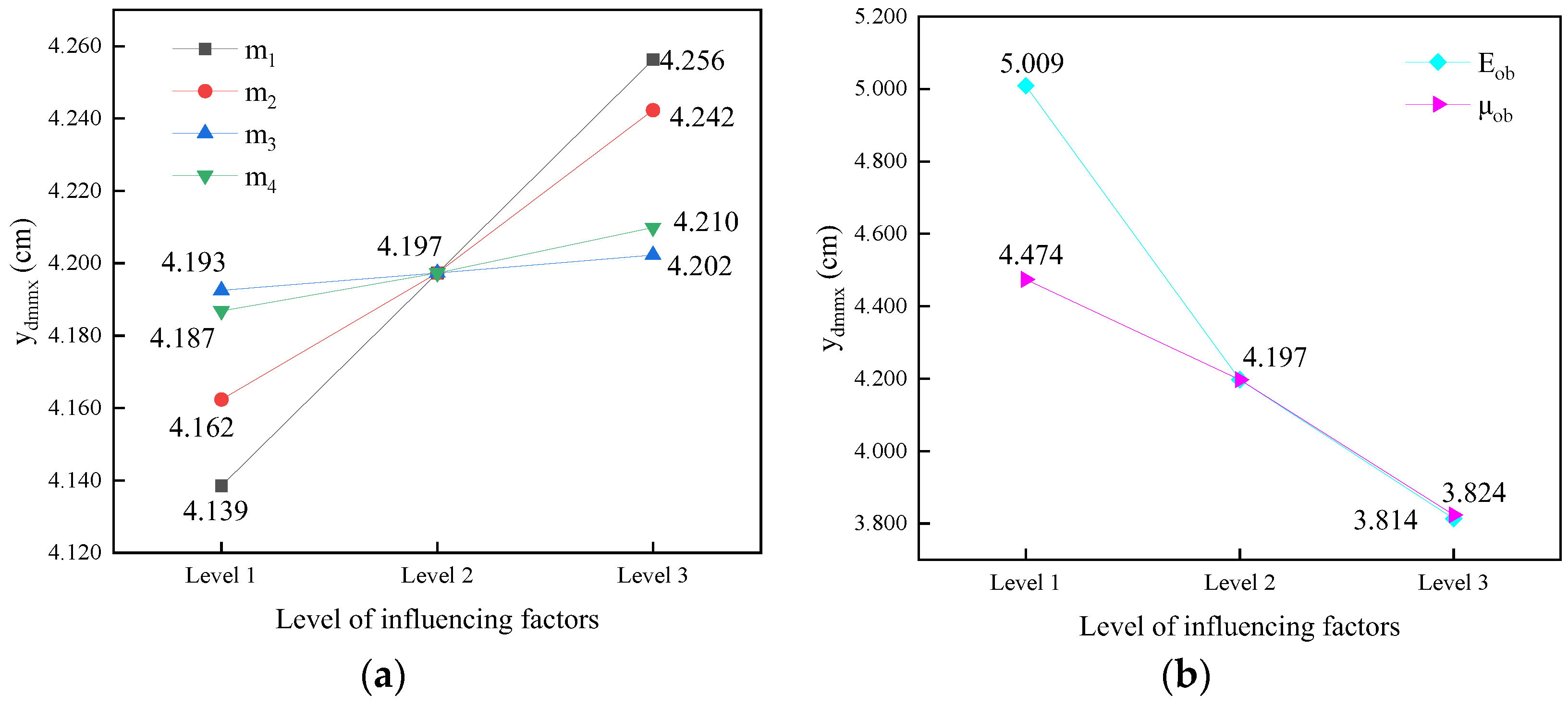
Figure 9.
Factors affecting maximum compressive stress. (a) Factors of geometric dimensions; (b) factors of performance of overburden.
Figure 9.
Factors affecting maximum compressive stress. (a) Factors of geometric dimensions; (b) factors of performance of overburden.
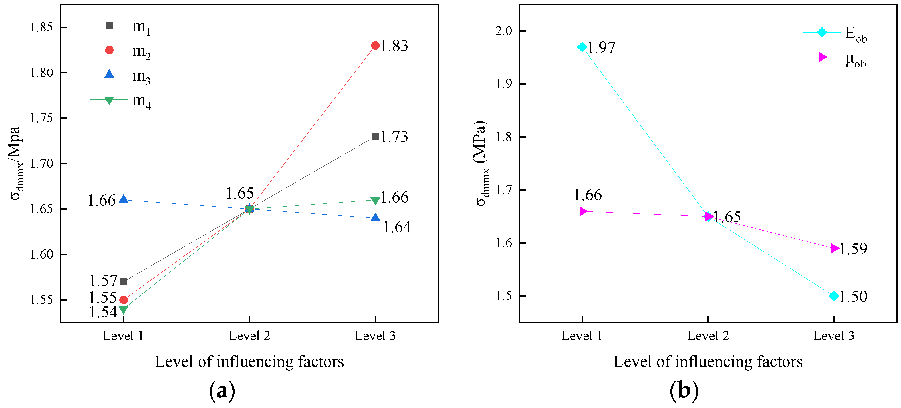
Figure 10.
Correlation between the selected parameters of numerical simulation and the maximum settlement and compressive stress of the CSG dam.
Figure 10.
Correlation between the selected parameters of numerical simulation and the maximum settlement and compressive stress of the CSG dam.

Figure 11.
Mean square error of the nodes in different hidden layers.
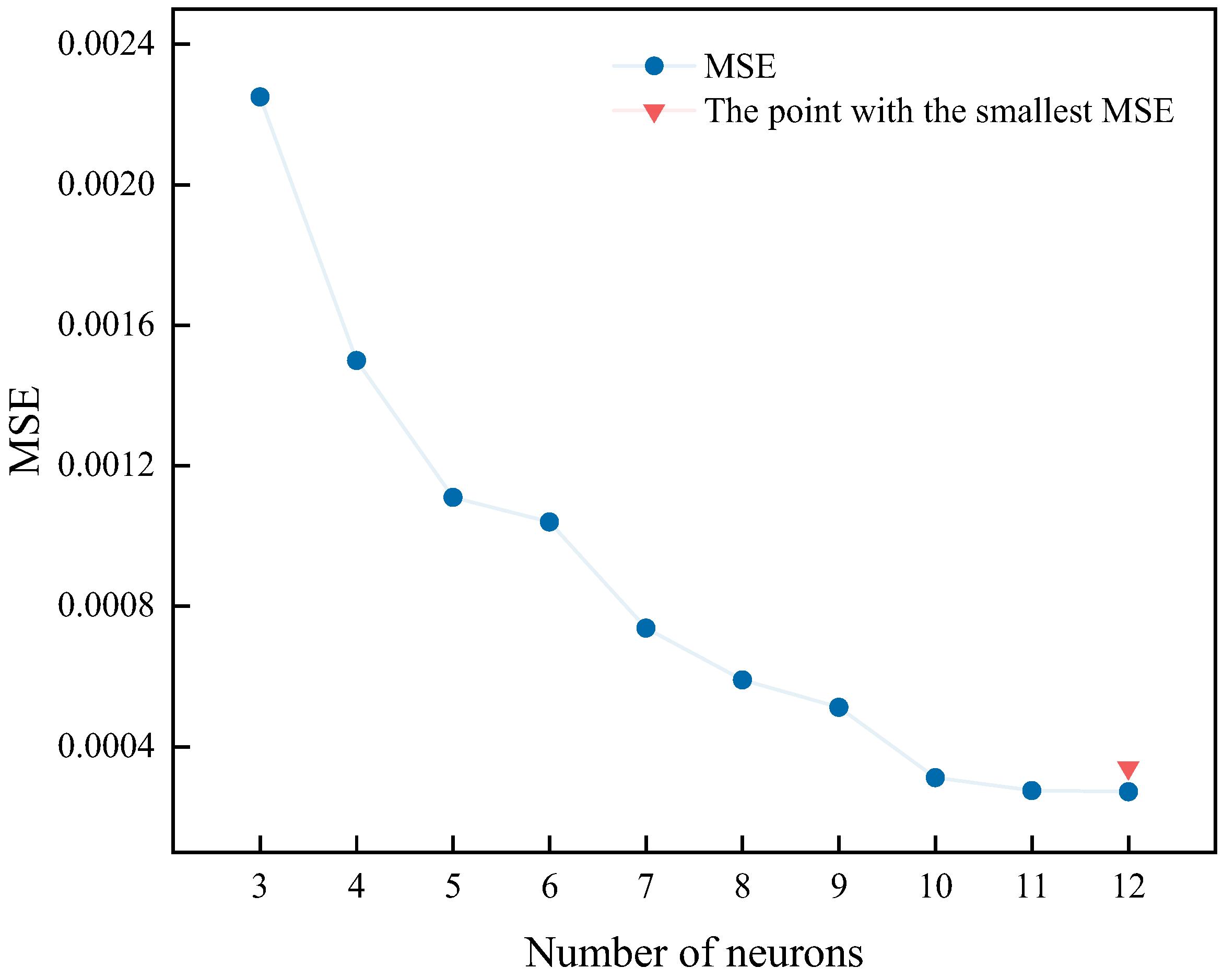
Figure 12.
Neural network modeling.
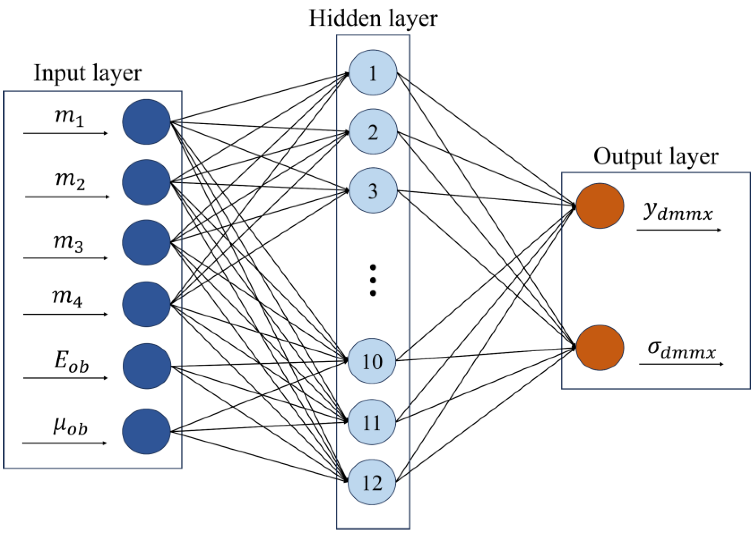
Figure 13.
Mean square error curve.

Figure 14.
Comparison of neural network prediction results. (a) For maximum settlement; (b) for maximum compressive stress.
Figure 14.
Comparison of neural network prediction results. (a) For maximum settlement; (b) for maximum compressive stress.
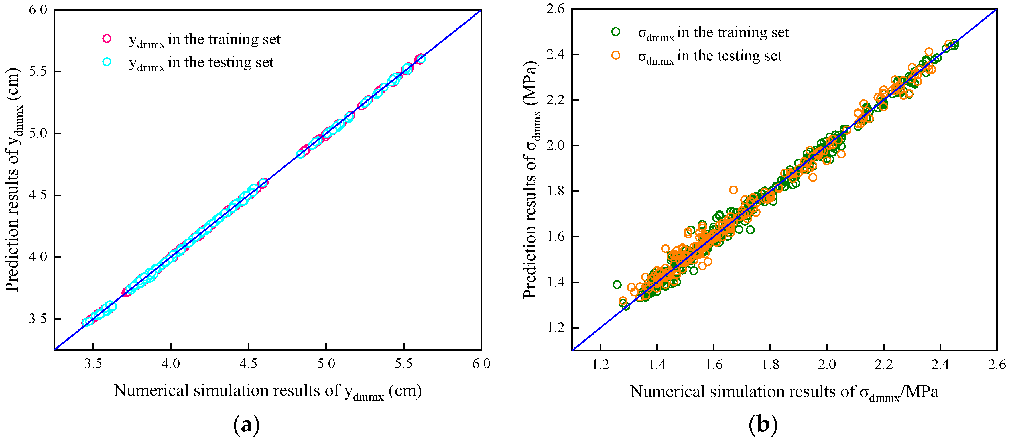
Figure 15.
Absolute error of neural network prediction results. (a) Section of training set; (b) section of texting set.
Figure 15.
Absolute error of neural network prediction results. (a) Section of training set; (b) section of texting set.

Figure 16.
Geometric dimension diagram of the dam body.
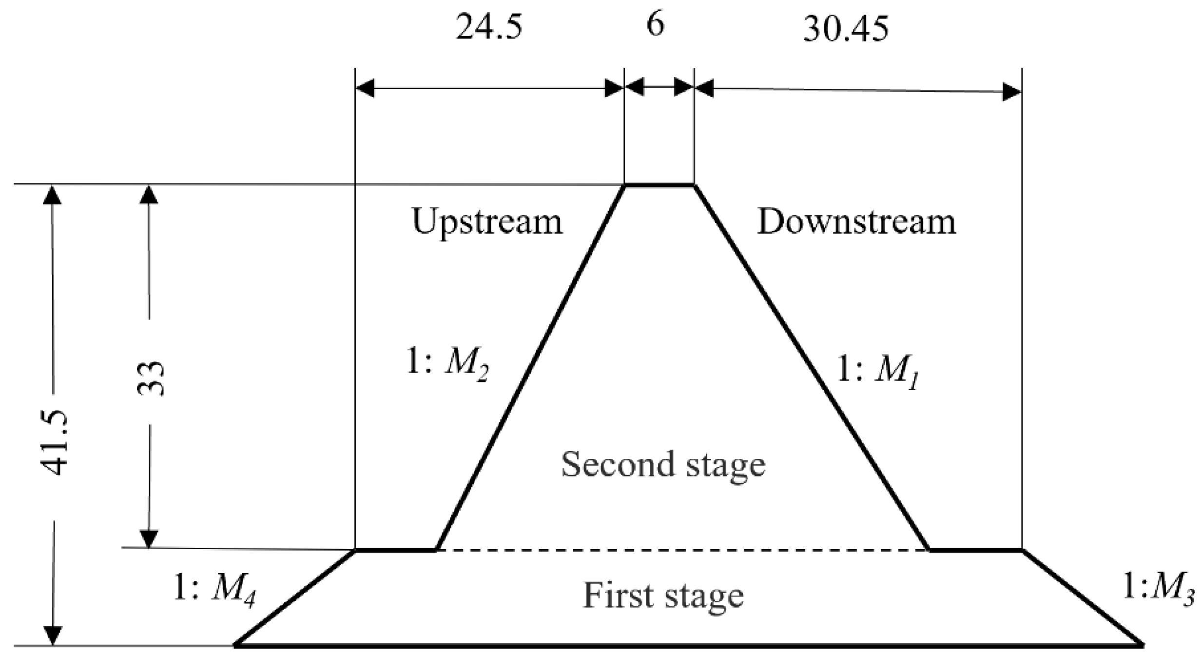
Figure 17.
Comparison of optimization methods. (a) Neural network combination method; (b) common method.
Figure 17.
Comparison of optimization methods. (a) Neural network combination method; (b) common method.

Figure 18.
Comparison of sections of optimized and initial dam.


Table 1.
Constitutive model parameters of dam body.
| Structure Name | (kPa) | (°) | ||||||
|---|---|---|---|---|---|---|---|---|
| CSG dam body | 1100 | 47 | 0.80 | 6400 | 0.35 | 0.30 | 0.01 | 0.30 |
Table 2.
Constitutive model parameters of overburden and bedrock.
| Structure Name | Density (kg·m−3) | Elastic Modulus (GPa) | Poisson’s Ratio | Cohesion (kPa) | Internal Friction Angle (°) |
|---|---|---|---|---|---|
| Overburden | 2200 | 1.2 | 0.4 | 5 | 36 |
| Bedrock | 2400 | 5.0 | 0.2 | - | - |
Table 3.
Characteristic values and positions of the dam body.
| Project | Maximum Displacement in the X Direction (cm) | Maximum Settlement in the Y Direction (cm) | Maximum Compressive Stress (MPa) | Maximum Tensile Stress (MPa) | |
|---|---|---|---|---|---|
| Completion period | Value | 0.132 (along the river direction) | 4.143 | 2.451 | 0.702 |
| Position | Toe of the first stage of the dam | Centerline of the dam crest | Junction of the first and second stages upstream of the dam | Upstream of the centerline of the dam bottom | |
| Impounding period | Value | 0.191 (along the river direction) | 4.190 | 2.412 | 0.671 |
| Position | Toe of the first stage of the dam | Upstream of the centerline of the dam crest | Junction of the first and second stages upstream of the dam | Upstream of the centerline of the dam bottom | |
Table 4.
Analysis of influencing factors and working conditions.
| Working Condition | (MPa) | |||||
|---|---|---|---|---|---|---|
| 1 | 0.5 | 0.55 | 1.05 | 1.05 | 1200 | 0.4 |
| 2 | 0.65 | |||||
| 3 | 0.8 | |||||
| 4 | 0.65 | 0.4 | 1.05 | 1.05 | 1200 | 0.4 |
| 5 | 0.55 | |||||
| 6 | 0.7 | |||||
| 7 | 0.65 | 0.55 | 0.6 | 1.05 | 1200 | 0.4 |
| 8 | 1.05 | |||||
| 9 | 1.5 | |||||
| 10 | 0.65 | 0.55 | 1.05 | 0.6 | 1200 | 0.4 |
| 11 | 1.05 | |||||
| 12 | 1.5 | |||||
| 13 | 0.65 | 0.55 | 1.05 | 1.05 | 700 | 0.4 |
| 14 | 1200 | |||||
| 15 | 1700 | |||||
| 16 | 0.65 | 0.55 | 1.05 | 1.05 | 1200 | 0.35 |
| 17 | 0.4 | |||||
| 18 | 0.45 |
Table 5.
Analysis of regression results based on BP neural network data.
| Project | Training Set | Test Set | ||||
|---|---|---|---|---|---|---|
| RMSE | MAPE | R2 | RMSE | MAPE | R2 | |
| 0.0095 cm | 0.18% | 0.9997 | 0.0109 cm | 0.21% | 0.9996 | |
| 0.0239 MPa | 1.03% | 0.9931 | 0.0335 MPa | 1.43% | 0.9871 | |
Table 6.
Check result.
(MPa) | (MPa) | (MPa) | (MPa) | (MPa) | ||
|---|---|---|---|---|---|---|
| Traditional method | −0.25 | −0.06 | 1.49 | 0.27 | 0.20 | 1.35 |
| Method based on BP | −0.26 | −0.11 | 1.51 | 0.39 | 0.35 | 1.11 |
| Requirement | <0 | <0 | <6 | - | - | <1.5 |
Table 7.
Effect of the optimization.
| Size | M1 | M2 | M3 | M4 | (cm) | (MPa) | (m3) | Time Consumption |
|---|---|---|---|---|---|---|---|---|
| Initial | 0.650 | 0.500 | 1.182 | 1.235 | 4.190 | 2.412 | 1429 | - |
| Optimization by traditional method | 0.517 | 0.403 | 0.651 | 0.647 | 4.083 | 1.492 | 1264 | 7 h 37 min |
| Optimization by method based on BP | 0.503 | 0.402 | 0.653 | 0.765 | 4.081 | 1.511 | 1260 | 4 h 30 min |
Disclaimer/Publisher’s Note: The statements, opinions and data contained in all publications are solely those of the individual author(s) and contributor(s) and not of MDPI and/or the editor(s). MDPI and/or the editor(s) disclaim responsibility for any injury to people or property resulting from any ideas, methods, instructions or products referred to in the content. |
© 2024 by the authors. Licensee MDPI, Basel, Switzerland. This article is an open access article distributed under the terms and conditions of the Creative Commons Attribution (CC BY) license (https://creativecommons.org/licenses/by/4.0/).
Share and Cite
MDPI and ACS Style
Wang, S.; Yang, H.; Lin, Z. Research on Settlement and Section Optimization of Cemented Sand and Gravel (CSG) Dam Based on BP Neural Network. Appl. Sci. 2024, 14, 3431. https://doi.org/10.3390/app14083431
AMA Style
Wang S, Yang H, Lin Z. Research on Settlement and Section Optimization of Cemented Sand and Gravel (CSG) Dam Based on BP Neural Network. Applied Sciences. 2024; 14(8):3431. https://doi.org/10.3390/app14083431
Chicago/Turabian StyleWang, Shuyan, Haixia Yang, and Zhanghuan Lin. 2024. "Research on Settlement and Section Optimization of Cemented Sand and Gravel (CSG) Dam Based on BP Neural Network" Applied Sciences 14, no. 8: 3431. https://doi.org/10.3390/app14083431
Note that from the first issue of 2016, this journal uses article numbers instead of page numbers. See further details here.