

Salient Object Detection via Fusion of Multi-Visual Perception
by
 , and
, and
Wenjun Zhou
1,*,
Tianfei Wang
1,
Xiaoqin Wu
1,
Chenglin Zuo
2,
Yifan Wang
1,
Quan Zhang
1 and
Bo Peng
1 1
School of Computer Science and Software Engineering, Southwest Petroleum University, Chengdu 610500, China
2
Key Laboratory of Icing and Anti/De-Icing, China Aerodynamics Research and Development Center, Mianyang 621000, China
*
Author to whom correspondence should be addressed.
Appl. Sci. 2024, 14(8), 3433; https://doi.org/10.3390/app14083433
Submission received: 17 March 2024
/
Revised: 16 April 2024
/
Accepted: 17 April 2024
/
Published: 18 April 2024
(This article belongs to the Topic Computer Vision and Image Processing, 2nd Edition)
Abstract
:Salient object detection aims to distinguish the most visually conspicuous regions, playing an important role in computer vision tasks. However, complex natural scenarios can challenge salient object detection, hindering accurate extraction of objects with rich morphological diversity. This paper proposes a novel method for salient object detection leveraging multi-visual perception, mirroring the human visual system’s rapid identification, and focusing on impressive objects/regions within complex scenes. First, a feature map is derived from the original image. Then, salient object detection results are obtained for each perception feature and combined via a feature fusion strategy to produce a saliency map. Finally, superpixel segmentation is employed for precise salient object extraction, removing interference areas. This multi-feature approach for salient object detection harnesses complementary features to adapt to complex scenarios. Competitive experiments on the MSRA10K and ECSSD datasets place our method in the first tier, achieving 0.1302 MAE and 0.9382 F-measure for the MSRA10K dataset and 0.0783 MAE and and 0.9635 F-measure for the ECSSD dataset, demonstrating superior salient object detection performance in complex natural scenarios.
1. Introduction
Attention plays an extremely important role in human perception systems [1]. Human visual perception often selectively disregards unnecessary information through attentional mechanisms. To effectively extract target information, it selectively attends to salient regions by integrating local contextual cues. The human visual system [2] is an important medium for human cognition of the world and has strong recognition and information processing capabilities. In the human visual system, humans can autonomously ignore a large amount of secondary and redundant information and further accurately locate and extract key information in the image. This key information can be perceived and refined to extract richer advanced information in the attention stage. Salient object detection imitates the human visual attention mechanism through computer calculation, with the aim of distinguishing the most visually attractive targets and quickly screen images by focusing on the target area that human eyes are most interested in [3]. Salient object detection is a binary classification problem, and its results need to highlight the boundaries and give complete targets. With the development of computer vision, this attention mechanism of the human visual system has attracted great interest. To detect more important and valuable information in images or videos, research on salient object detection is gradually emerging, with the aim of highlighting the most salient objects in an image [4]. Such research holds practical significance for applications including video surveillance, virtual reality, human–computer interaction, and autonomous navigation. Over the past few decades, many approaches have been proposed to detect salient objects [5]. In general, there are two main methods for salient object detection: bottom-up and top-down [6,7,8,9].
Bottom-up approaches are fast, data-driven, and task-dependent [10] and are usually based on easy-to-implement primitive features such as color, intensity, and texture. However, salient objects cannot be detected using these features alone. Therefore, bottom-up methods make some assumptions about object and background properties, including the contrast prior, center prior, and background prior [11]. For example, the contrast prior assumes that salient regions are always different from their neighbors or scenes and can be further divided into the local contrast prior and global contrast prior [2], the center prior is established based on the fact that salient objects are more likely to exist in the center of the image, and the background prior indicates that the boundaries of the image are more likely to be part of the background. With these assumptions, salient regions can be better highlighted with background suppressed.
In addition, top-down approaches are slow, well-controlled, and task-driven and require supervised learning [12] based on manually labeled training samples. With the development of deep learning methods, this method has achieved great success in salient object detection. Deep-learning-based algorithms [13,14] can process semantic-level or image-level features of training samples and achieve the best performance for saliency detection. However, deep neural networks require a large number of labeled samples to iteratively adjust massive training parameters, have a long training process, and cannot be applied to online learning. For example, commonly used CNN (convolutional neural network) architectures, such as ResNet-50 [15] and VGG16 [16], have a large number of parameters. ResNet-50 has over 20 million parameters, while VGG16 has approximately 130 million parameters. The time required to complete a full training and inference cycle is incomparably longer than the method proposed in this paper. Therefore, most existing deep-learning-based methods are time-consuming and highly reliant on well-annotated training datasets [10]. Besides the efficient training problem, labeling a large number of samples is also a difficult task in practice [6].
To tackle the problems mentioned above, this paper proposes a bottom-up-based salient object detection method using multi-visual perception. Most of the intuitive perception of human vision is unsupervised and mostly based on low-level visual features such as color, texture, and brightness. Contrast, as a very important feature for salient region recognition, has a critical impact on visual effects. The greater the contrast, the clearer and more eye-catching the image is, and the easier it is for human eyes to notice the object. The reason why salient objects can attract the attention of the human visual system is that their feature performance is different from the surrounding environment. Therefore, this paper mainly uses five different low-level visual perception features: gradient feature, mean subtractive contrast normalization (MSN) coefficients [17], the dark channel, saturation, and hue to detect salient objects by analyzing the visual presentation characteristics of natural images. More details are described in Section 3.1 and Section 3.2. The method follows the feature utilization of the human visual system when recognizing objects in images. First, saliency maps are acquired by every single feature, then fused through an effective strategy, and finally combined with superpixel segmentation to obtain the final result. During the experimental phase, we utilized two challenging datasets, MSRA10K [18] and ECSSD [19], and evaluated our method using common precision–recall (PR) curve, ROC curve, F-measure, and mean absolute error (MAE) metrics. Detailed descriptions of the specific evaluation procedures are provided in Section 5.1 and Section 5.2. In short, the main contributions of this paper are as follows:
- (1)
- Methodology for salient object detection: The paper introduces an innovative approach to salient object detection, leveraging multi-visual perception. This pioneering method capitalizes on the synergy of various visual cues to enhance accuracy.
- (2)
- Enhanced feature utilization: By incorporating five distinct low-level visual features, the proposed method significantly bolsters its ability to handle intricate natural scenes. These nuanced features contribute to robustness and adaptability.
- (3)
- Coherent framework for accurate detection: The integration of multiple features within a coherent framework yields substantial improvements in salient object detection. Notably, this leads to a pronounced reduction in both false positives and false negatives.
In summary, our method fully utilizes the underlying representation features of images, thoroughly explores and integrates global and local characteristics, and achieves good performance without requiring costly training data or teacher signals.
The remainder of this paper is organized as follows. Section 2 discusses related work, and Section 3 explains the motivation and background for our work. Section 4 presents the details of our proposed method. Then, Section 5 describes experiments demonstrating the proposed method’s performance. The explanation of experimental results and further validation of the proposed method are expanded upon in Section 6. Finally, Section 7 concludes.
2. Related Work
Over the past two decades, salient object detection methods have developed rapidly. Vision-based object detection is an interdisciplinary research topic in image processing, computer vision, and pattern recognition [4]. Some strategies for salient object detection use unsupervised techniques by combining visual features and prior theory. The earliest creative method proposed by Itti et al. [20] was based on color, intensity, and contrast around the center of the orientation. Then, Jiang et al. [21] introduced a regional-level saliency descriptor primarily constructed on local-contrast, background, and other well-known features. Achanta et al. [22] described a frequency-adjusted global-contrast-based method to measure saliency. Yang et al. [23] used a graph-based approach to measure the similarity of regions to foreground or background cues through the boundary prior and manifold ordering. Jia and Han [24] calculated the saliency scores for each region and then compared them to the soft foreground and background. Liu et al. [25] utilized a Bayesian framework for saliency detection based on a Bayesian model. To overcome the limitation of using only contrast, Lou et al. [26] proposed the use of statistical and color contrast to detect salient objects. Furthermore, there are some successful examples salient object detection by combining visual features with prior theory [27,28,29].
With the boom in deep learning [12], saliency detection has introduced supervised learning methods. Among them, it is worth mentioning the region-based CNN model and the FCN-based (fully convolutional networks) model. Region-based methods [14] divide the input image into multi-scale or smaller regions and use CNNs to extract their high-level features. Then, the multi-layer perceptron (MLP) outputs the saliency value of each small region through these high-level features. Although region-based CNN models have achieved good performance, these models cannot preserve spatial information due to small region segmentation. Therefore, an FCN-based method was designed to overcome this shortcoming [13]. This method operates at the pixel level rather than at the region or patch level. It overcomes the limitations of region-based CNN models and also preserves contextual information well. However, substantial labeled data with teacher signals or ground truth is necessary for their training, leading to inherent computational complexity and potential unavailability.
The traditional methods mentioned above typically focus on a limited set of features, such as local contrast and color contrast, resulting in under-utilization of image information. Deep learning methods typically extract semantic features through convolution, neglecting surface-level features of images. Additionally, they perform convolution at the block level, overlooking the consideration of connectivity between salient objects across blocks. Furthermore, they require a large amount of annotated data, which is time-consuming and labor-intensive, and the complexity of networks results in high time complexity.
To address the aforementioned challenges, this paper proposes a multi-feature detection method leveraging the rich features of images. Employing multiple features is not only beneficial for saliency detection in complex natural scenes but also mitigates limitations of single-feature approaches. Moreover, the proposed bottom-up method is simple and data-independent.
3. Motivation and Background
3.1. Motivation
The generation of visual saliency arises from the formation of a new and distinct stimulus that captures the observer’s attention due to the contrast between visual objects and the surrounding environment. This results in visual contrast, often induced by the elements constituting the image itself. Regions with higher contrast are more likely to attract the visual system’s attention and are referred to as salient regions, while visual stimuli are described through features [30].
Generally, an image feature describes a visual attribute of a specific aspect of the image object. Different dimensions of features can describe the image from various perspectives [30], such as contours of different subjects, texture features, brightness contrast depicting sensory depth, and distant/nearby objects, while color features aid in object recognition and differentiation. The human eye comprehends images through the integrated analysis of multiple perceptual features to achieve a final understanding of the image. To simulate human visual mechanisms, multiple features are selected. For instance, MSCN and gradient features describe the texture distribution in the image. Given the heightened sensitivity of the human eye to edges and textures, these features contribute to simulating such sensitivity, thereby enhancing the perceptual quality of the image. The dark channel, mapping the minimum pixel values in the image, is employed to extract depth information from the scene, simulating human perception of image depth and relative distances between objects. In natural environments, objects often possess unique colors, aiding in the perception and memorization of the surroundings. Colors serve as crucial identifying features for remembered objects and scenes.
The aforementioned features collectively cover almost all the information acquired by the human visual system [31], leading us to integrate MSCN coefficients, gradient feature, dark channel, saturation, and hue features to emulate the human visual perception system.
3.2. Visual Perceptual Features
The proposed method uses five different perceptual features, i.e., gradient feature, MSCN coefficients, the dark channel, saturation, and hue in the HSV color space. These perceptual features play an essential role in the human visual recognition process. The details of each perceptual feature are described as follows.
Gradient feature: The human visual system recognizes objects by their edges. The higher the value in a gradient image, the closer to the edge observed by human vision. The gradient feature uses edge detection operators to extract texture information from images and represent it as finer object structures. In this work, a robust contrast operator [32] (:contrast value operator) was used for gradient feature extraction.
MSCN coefficients: Due to the smooth transition of image regions, adjacent pixels of natural images tend to have high correlations. The human visual system detects salient objects after removing this high correlation. The MSCN coefficients are proven to reduce image region correlation [33]. Therefore, an MSCN coefficient feature map can decorrelate salient objects with their surroundings. The MSCN coefficients are calculated as follows:
where and are spatial indices. is a 2D circularly symmetric Gaussian weighting function sampled to three standard deviations () and rescaled to unit volume. is the gray version of a raw image I.
In addition, we find that the distribution of the salient object values tends to be concentrated in part of the MSCN coefficient feature value. So, the feature map is combined with the histogram to detect salient objects.
Dark channel: Although the dark channel prior is first proposed in the direction of dehazing, some papers have studied its feature to detect salient objects. Refs. [34,35] demonstrated that the dark channel prior could effectively suppress detection failures due to large background regions, foreground touching image boundaries, and the foreground and background sharing similar color appearances.
The dark channel is a kind of statistical characteristic of outdoor haze-free images because the study found that in most non-sky patches, at least one color channel has some pixels with very low pixel intensities close to zero [36]. It is obtained as follows:
where is a color channel of I and is a local patch centered at x.
Saturation: Saturation can represent how color density drops from the maximum value to 0. The purer the color, the higher the saturation, and high saturation equals high recognizability of colors.
Hue: Hue is considered to be the primary characteristic of color. Changing the hue will lead to a more considerable difference than changing the same amount of saturation or value [11]. Therefore, color is also an important perceptual feature when human eyes focus on salient features.
Five feature maps with size are obtained from the original image, gradient feature , MSCN coefficients , dark channel , saturation , and hue . To improve the detection efficiency while preserving the effective information of the feature maps, the feature maps are downsampled to the maximum value. In this work, the downsampled feature maps were obtained by K-fold maximum downsampling with the size of . Then, the downsampled maps are normalized as follows:
4. Methodology
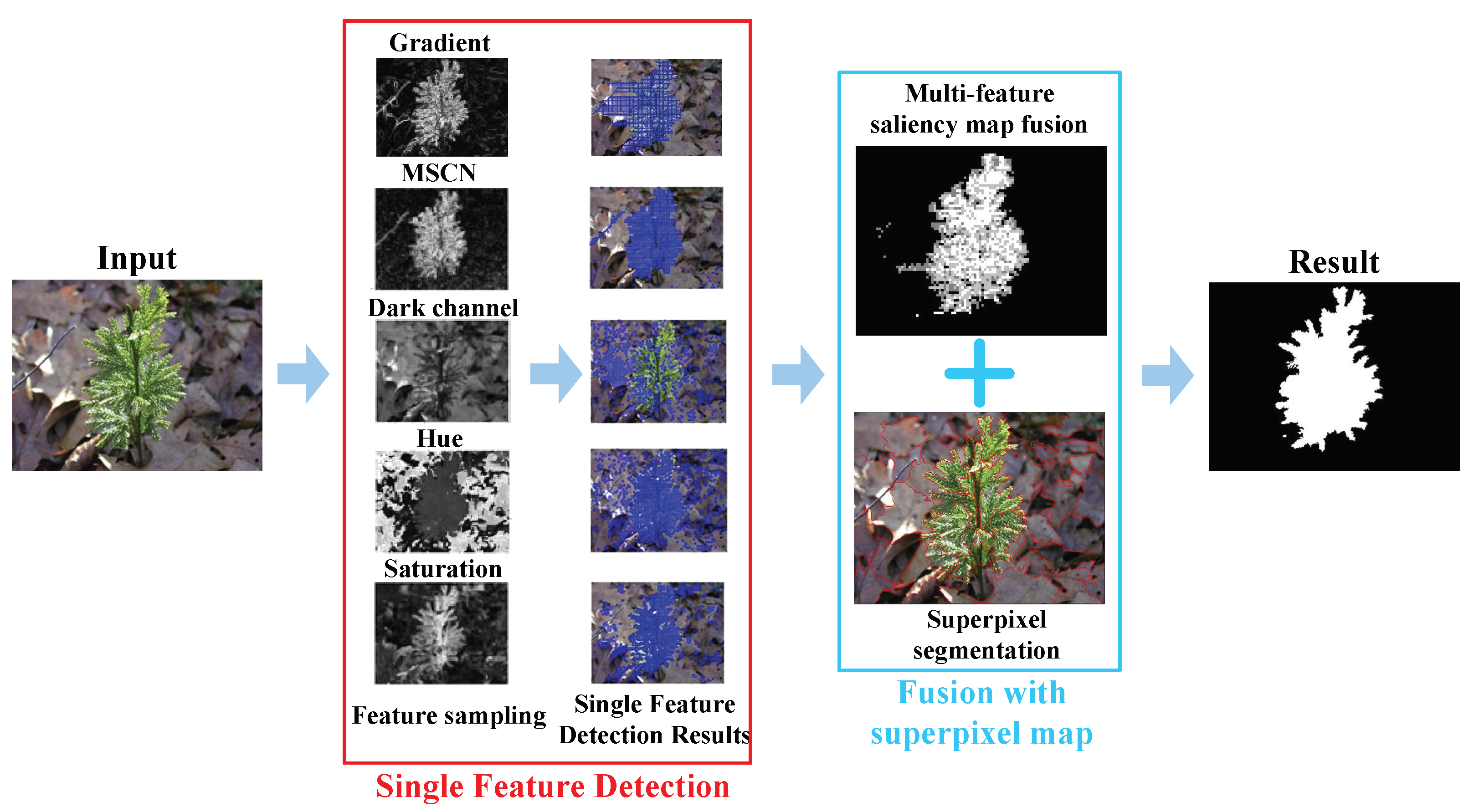
In reality, human visual systems can acquire various kinds of information for object recognition. Therefore, the method proposed in this paper simulates the recognition process of human vision through a variety of perceptual features. The framework of our method is illustrated in Figure 1. First, the saliency map corresponding to each perceptual feature is detected. Second, the saliency maps with different perceptual features are merged into one with an effective strategy. Third, the superpixel segmentation is involved in generating the final saliency map.
4.1. Single Feature Detection
Humans have an inconsistent understanding of different features, so it is impossible to use the same detection method for each feature. According to the characteristics of each feature, different detection strategies are designed to acquire the different saliency maps of every single-feature.
Gradient feature: Gradient values are usually large at the contours of salient objects, so gradient features are selected to detect salient objects. During gradient feature map detection, salient objects are obtained by finding salient object edges row by row. First, each row of data is put into a chart, and its peak points are found, likely to be the edges of salient objects. In this paper, peak points larger than are considered as the edges of salient objects, where is the maximum value of the whole map, and is set to 0.45. Then, salient regions are identified through those peak points. If the peak points are concentrated, the space between the concentrated peak points is a salient area. Finally, salient objects can be obtained according to the salient regions of each row. Figure 2 illustrates the gradient feature detection process. Figure 2b shows one row of gradient changes taken from Figure 2a. In addition, the peak points larger than with an asterisk are marked, and the salient region of this row is obtained. Figure 2c shows the saliency map obtained by gradient features.
MSCN coefficients: By studying the characteristics of MSCN coefficients, we note a significant difference in the MSCN distribution between salient objects and the background, as shown in Figure 3.
In this paper, it is defined as the statistical histogram as the discrete function:
where represents the value of level k, and is the number of in the image. Then, the corresponding statistical histogram can be obtained through the feature map of MSCN coefficients as Equation (6). The histogram is normalized as follows:
where estimates the probability that the value appears in the MSCN coefficient feature map. When the histogram distribution satisfies one of the three conditions, the value range greater than is chosen as the distribution range of salient objects. If none of the above three conditions are satisfied, the distribution range of salient objects is in a region less than . The initial value of is set to 0.4. If the salient region obtained by the initial value is small, is changed to enlarge the salient region. The three conditions are as follows:
- (1)
- , where , means that more than of the MSCN coefficient maps values are in the front four levels;
- (2)
- means that the first level is the maximum value of the statistical histogram;
- (3)
- The maximum value of the statistical histogram is in the first four levels, and exceeds eight levels;
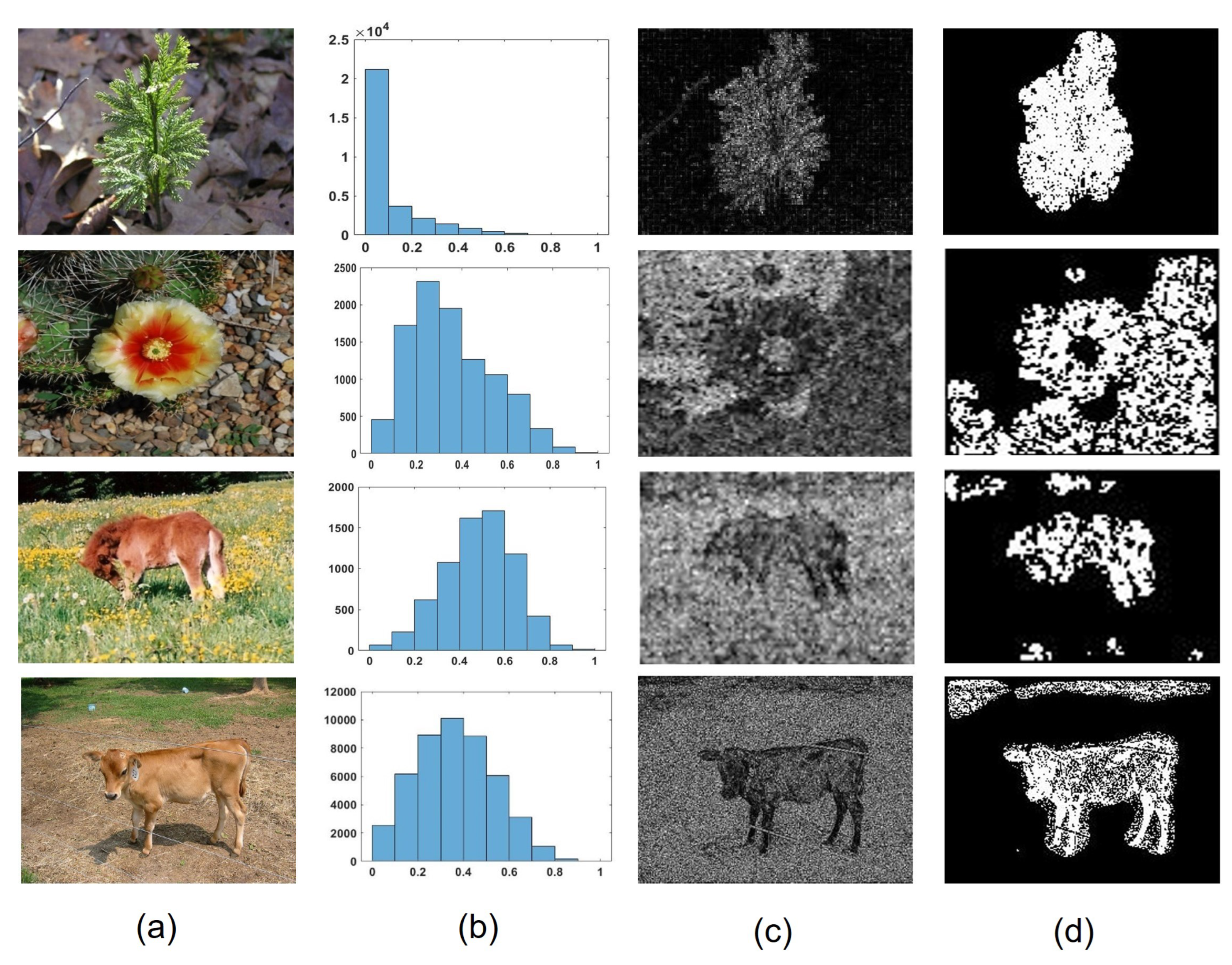
Figure 4 shows some examples of MSCN coefficient detection, where the histogram distribution of the first image satisfies one of the above three conditions, so the range greater than is the salient object distribution range. The other images do not meet the three conditions, so the range less than is the salient object distribution range. Figure 4c shows the detection result of the image.
The three other features, dark channel, saturation, and hue: The statistical histogram is combined with the background prior theory [28] to detect salient objects. In most scenarios, the background prior theory assumes that the edges of the image tend to be the background. Thus, the edges of the image are considered non-salient. Therefore, when the statistical histogram changes from the edge to the whole, the newly emerging values are also almost salient object values. In addition, there are sometimes salient objects at the edges of the image, so when the statistical histogram values increase from the edges to the overall anomaly, these values are also likely to be salient object values. To obtain the value of salient objects, first, the statistical histogram of is defined as , where . Second, the outermost value of the four sides of is extracted, and its statistical histogram is obtained as . The statistics of each level are then processed as a whole/edge to obtain the pixel increase multiplier for each level, and its expression is as follows:
Through the multiplier, the saliency map can be obtained as follows:
where means a value that does not exist in but exists in . is a threshold for judging whether the value increases abnormally in the process from the edge to the whole, where means to find the mean value of , means to find the variance of , and is set to 1.5. Here, the threshold T varies with the values of the mean and variance. If the histogram level of the feature map value satisfies the above two conditions, it is set to 1. Otherwise, it is set to 0. As one example, Figure 5 illustrates the feature of the hue detection process. Figure 5a shows the statistics histogram of . Figure 5b shows the edge statistics histogram of . Figure 5c is the hue growth result from the edge to the whole image calculated by Equation (8). Figure 5d is the hue’s final saliency map. The features of the dark channel and saturation also follow the same process.
4.2. Fusion with Superpixel Map
For individual images, feature maps are determined based on the histogram distributions of different features. After obtaining feature maps through features, these feature maps are fused. Algorithm 1 shows the feature salient object fusion process. There are some non-salient points in each feature saliency map. Therefore, for accurate detection, we fuse the multi-perception features to calculate the final accurate feature map. It first calculates the density of salient points around each salient point of each feature saliency map . The specific calculation method draws a rectangle centered on the point, calculates the salient point density in the rectangle, and obtains the salient density. After obtaining the saliency density of each saliency point, the saliency points whose saliency density is less than are regarded as noise points and removed, and is set to as the best value obtained from experiments. Then, the feature saliency maps after denoising are fused as the fused saliency map . For any given image, the probability of meeting the foreground conditions using these three features is higher for the foreground. Therefore, we have assigned an equal weight ratio of 1:1 to each feature. Ultimately, the identification of three or more features as meeting the foreground criteria defines this area as the foreground. Then, the fusion process involves adding the values of the five feature saliency maps, where pixels with a sum greater than or equal to 3 are considered foreground, while those below 3 are considered background. Ultimately, the resulting saliency map is represented as . Finally, an inverse up-sampling process is presented on the fused saliency map, restoring it to the input image size. The final fused saliency map of Figure 6a is shown in Figure 6b as one typical example.
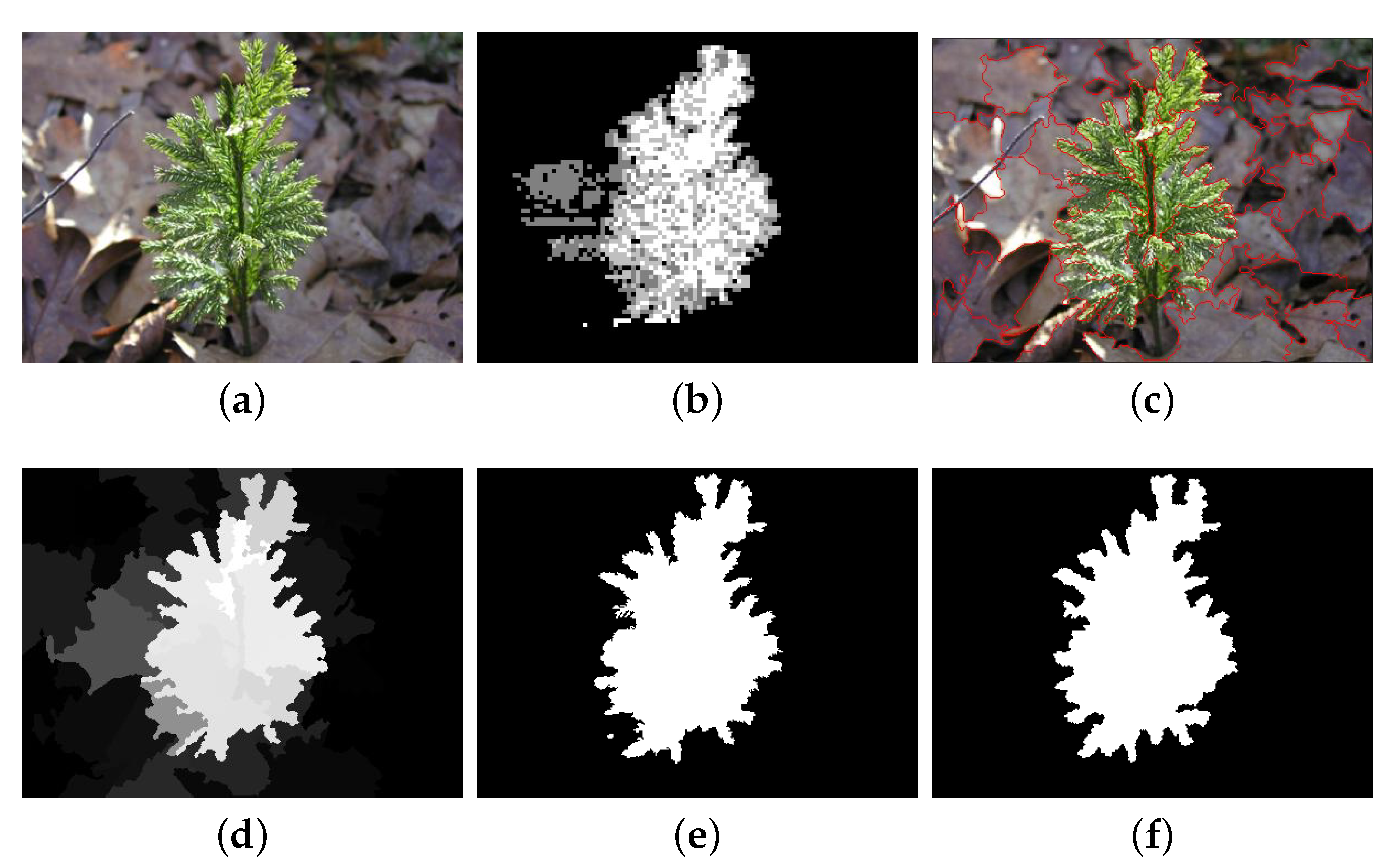
As can be seen from Figure 6b, the edges of salient objects are relatively rough, so the superpixel segmentation algorithm is introduced for refinement. Here, the SLIC superpixel segmentation algorithm [37,38] is involved in removing the interference area to obtain the final salient object. In this paper, the fusion strategy of SLIC is improved by considering both the color and area of superpixel blocks when fusing superpixel blocks. As before, the SLIC algorithm is first used to segment the image [38]. Then, the blocks are fused with a small color difference, and the area of the fused blocks is judged. If the area of the block is too small, it is fused with the surrounding superpixel block with the smallest chromatic aberration. After each superpixel segmentation block is processed through the above steps, the final superpixel segmentation map can be obtained. Figure 6c is the final superpixel segmentation map of Figure 6a.
| Algorithm 1 Multi-perception feature map fusion |
|
The final superpixel segmentation map splits the image into many superpixel blocks. The mean value of each superpixel block is calculated as its saliency value, i.e., , where c is the index of the superpixel block, is the superpixel block with index c, and represents the mean value of the saliency of the pixel block. The saliency map is then obtained by normalizing saliency values, as shown in Figure 6d and binarized using SC’s adaptive threshold method [18]. The resulting binary map is shown in Figure 6e.
5. Experiments
All experiments were run with an AMD Ryzen 7 5800X 8-Core and 32 GB RAM on MATLAB (R2021b) platform.
5.1. Evaluation Metrics
To comprehensively evaluate the performance of the algorithm, four quantitative evaluation indicators are used: the precision–recall () curve, ROC curve, F-measure, and mean absolute error ().
The binary maps are obtained from the saliency maps by applying a threshold from 0 to 255. Then, the precision (P) and recall (R) value pairs are obtained from these binary images and the ground truth, and a curve is plotted. P and R can be calculated as:
where B is the binary map, and is the ground truth.
The ROC curve is the curve obtained by the false positive rate (FPR) and true positive rate (TPR). FPR represents the probability of mispredicting a positive sample among all negative samples, while TPR means the probability of being correctly predicted as a positive sample among all positive samples.
The F-measure is also obtained through the P-R value pair, which is calculated as:
where , indicating that improving precision is more important than improving recall.
Mean absolute error () is a simple and reliable binary map evaluation metric. It is computed as the mean of the pixel-level absolute error between the binary map (M) and the corresponding , defined as:
where M and N represent the height and width of the image, respectively.
5.2. Datasets
Two challenging public datasets were adopted for detection and evaluation in this work. The MSRA10K dataset [18] is a large image dataset containing 10,000 images, where each image contains a salient object or a unique foreground object. The image content of the database is varied, but the background structure is mostly simple and smooth. It is the first dataset for the quantitative evaluation of salient object detection.
The ECSSD dataset is an extension of the CSSD dataset [19]. It consists of complex scenes that exhibit textures and structures common in real-world images. The dataset contains a total of 1000 complex images and their respective ground-truth saliency maps [39].
In this work, the pixel-level ground truth was employed to evaluate the MASR10K and ECSSD datasets, which achieved more accurate results than the bounding-box-based ground truth.
5.3. Ablation Experiments
In this study, multi-visual perception features were employed for salient object detection. To verify the positive facilitation effects in the multi-visual perception salient object method, ablation experiments were conducted by only selecting one feature from multi-visual perception features. PR evaluation metrics of each feature detection result on the ESSCD dataset are shown in Figure 7. This experiment proves that each perceptual feature can detect salient objects but is ineffective. From the experimental results, it should be noted that when all perceptual features work together, the salient object detection method can be more suitable for complex natural scenarios.
5.4. Results
The results of the proposed method for ECSSD and MASR10K datasets were compared with those of MSS [40], COV [41], GR [42], PCA [43], LDS [44], FCB [45], CNS [26], MDF [46], PPMRF [47], saliency bagging [2], MTL-ITSOD [48], PDLSO [7], and LC-SA [6] methods. These algorithms were selected to demonstrate the performance of our proposed method. The methods of Refs. [40,41] can combat complex natural scenarios and [42,43], based on the prior theory, make results more robust. Others [26,46,47] are representative methods that emerged in recent years. All these methods utilize color and some prior theories to suppress background information and highlight salient objects. The parameters settings in our work are shown in Table 1.
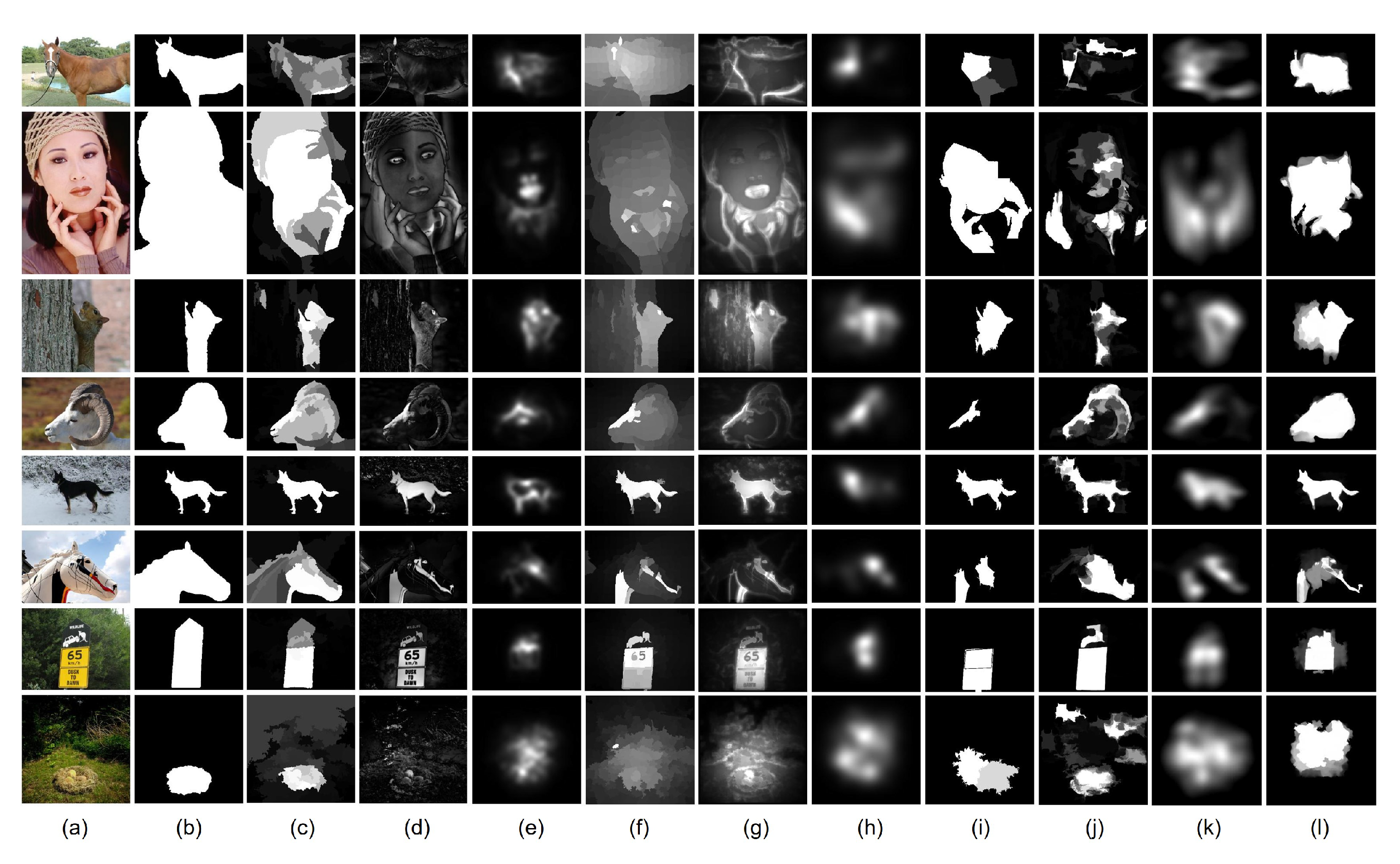
The visual comparison of all evaluated methods is shown in Figure 8. The saliency maps generated by our method are more consistent with the ground truth. Our method can better suppress background noise and highlight salient objects.
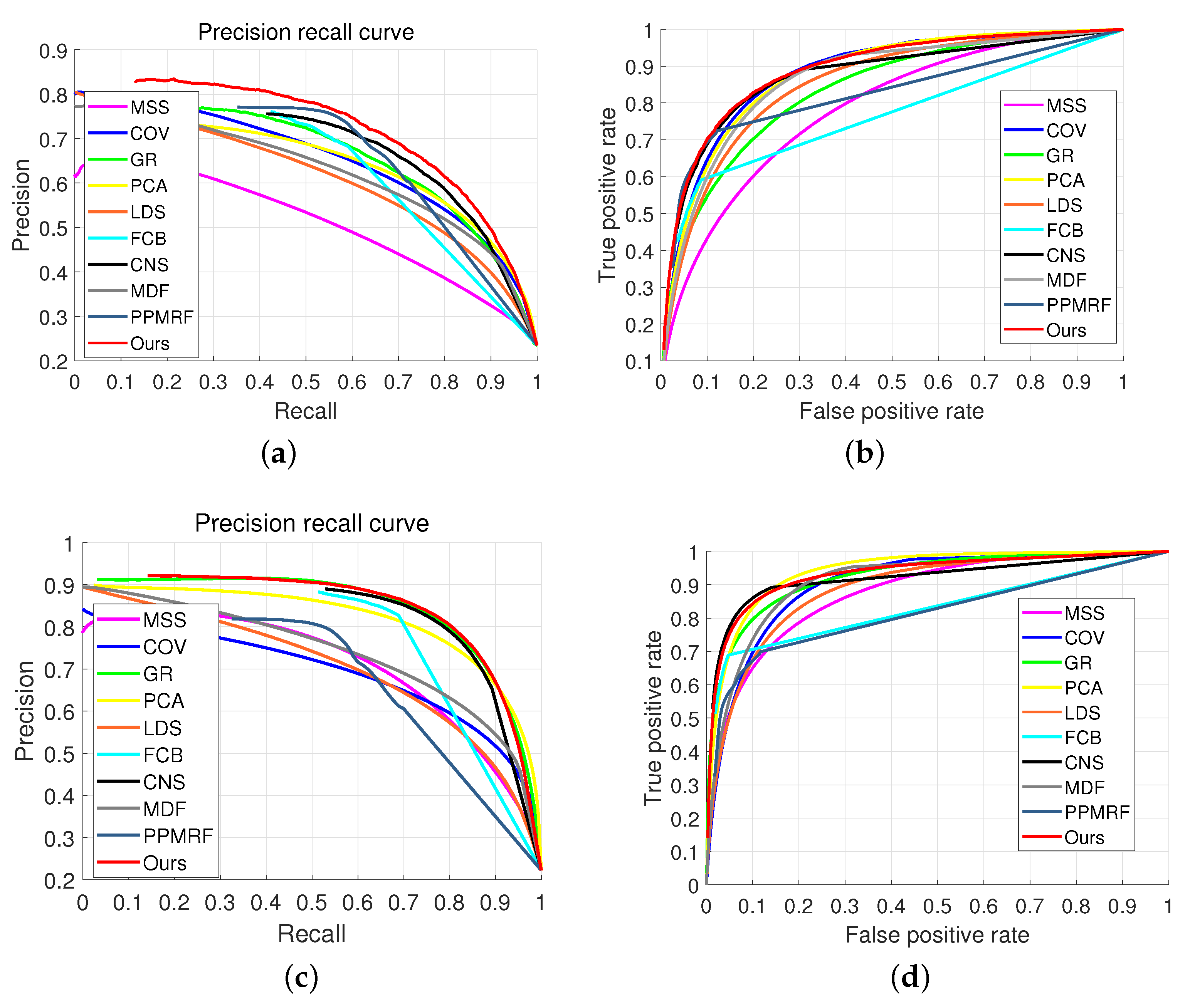
In Figure 9, saliency maps are evaluated through PR and ROC curves to show the performance of our method. The curve of our method is above that of other methods, which shows that our method leads the way compared with others.
Moreover, to further clarify the advantages of our approach relative to existing methodologies, we performed comparisons based on quantitative metrics (F-measure and MAE) with the MSS [40], COV [41], GR [42], PCA [43], LDS [44], FCB [45], CNS [26], MDF [46], PPMRF [47], saliency bagging [2], MTL-ITSOD [48], PDLSO [7], and LC-SA [6] methods using the ECSSD and MSRA10K datasets. Notably, due to the absence of results for the MTL-ITSOD and PDLSO algorithms for the MSRA10K dataset and the lack of results for the LC-SA algorithm for the ECSSD dataset, these instances are indicated in the table with a hyphen. Analysis of the MAE and F-measure results from Table 2 reveals commendable performance of our proposed method for both the ECSSD and MSRA10K datasets.
5.5. Time Complexity Analysis
The input image has dimensions of pixels, and the program executes times, where is a constant. In the feature extraction phase, each of the five features requires a constant number of operations on each pixel. The time complexity of the feature extraction phase is . The feature fusion phase involves adding the feature maps obtained from feature extraction and performing binary thresholding. This requires processing each pixel in each of the five feature maps, resulting in a time complexity of for the feature fusion module. The superpixel segmentation utilizes the SLIC algorithm with a time complexity of . Therefore, the overall time complexity of the proposed algorithm is .
The proposed method processes images of 300 × 400 pixels in an average time of 2.1 s on an AMD Ryzen 7 5800X 8-Core CPU with 32 GB RAM using MATLAB. This speed is due to MATLAB’s serial processing, where the single-core processing capability of the CPU affects the algorithm’s runtime. Theoretically, using more advanced CPU processors, our algorithm will achieve a higher processing speed.
We compared the COV algorithm [41], also implemented in MATLAB, with an average runtime of approximately 3.6 s. However, compared to the GR algorithm [42], the runtime is approximately 0.8 s, owing to the higher efficiency of GR using C++ code. Additionally, our method extracts more low-level image features, which consequently increases the computational workload.
Time complexity analysis suggests the method’s computational demands correlate linearly with the product of the image dimensions. The method’s efficiency, demonstrated by execution time on specific hardware, supports viability for real-time or near-real-time image processing applications.
6. Discussion
6.1. Parameter Settings
By analyzing the distribution of various visual perceptual features for nature images, we fully leverage low-level image characteristics to identify salient objects. For example, using the MSCN feature, we found that most salient regions account for 30–50% of total MSCN features, while non-salient regions typically account for 70% (see Figure 10b,c. Peak values are mostly near 0.4, so we set to 0.7 and ’s initial value to 0.4.
On the other hand, regarding the H channel, salient regions often exhibit significant H value differences from edges (see Figure 10d–f). We calculate each H value’s occurrence count in the original image divided by its count in edges. We believe a salient region’s growth ratio must exceed the average. If its standard deviation is large, it indicates one or more peaks. These H channel features in peak regions are what we aim to capture, so we set to 1.5 to better obtain salient regions using the H channel.
6.2. Results Analysis
In ablation experiments, the curve for the multi-visual perceptual feature detection method lies above all other curves, indicating that this approach is more effective and versatile than single-feature detection methods. Moreover, when designing detection methods for each single feature, we emphasize their contribution to the whole method. Consequently, methods relying on a single feature cannot adapt to all complex natural environments and perform poorly on the dataset.
It is worth mentioning that these results are sufficient to demonstrate that these features can be applied to salient object detection. Visually, our method can detect salient objects more completely and accurately than other methods. Quantitatively, some comparison methods outperform our method on some evaluation metrics. For example, the F-measure for the ECSSD and MSRA10K datasets in Table 2 is not optimal among all methods. The reason for this is that the detection method of multiple feature fusion has yet to be optimized. In particular, the MSCN feature map using feature statistical properties summarizes three conditions for detecting salient objects. These three conditions only cover most conditions and need further refinement in the future.
Furthermore, with the help of multiple perceptual features participating in salient object detection without relying on a single feature, this method shows effectiveness in complex scenarios. Additionally, the denoising operation and superpixel segmentation method achieve stronger performance.
6.3. Performance with Low Resolution
To further validate our method’s effectiveness for low-resolution images, we conducted relevant experiments. Testing across different image resolutions yielded typical results as shown in Figure 11. Our method performs well across various low-resolution images. However, as resolution decreases further, detection becomes increasingly affected by background interference, making background areas easier to detect. When resolution reaches its limit, such as 200 × 150, subtle feature detection, including shape structures and fine edges, is impaired, lowering detection accuracy. Nevertheless, salient areas remain recognizable. Therefore, our multi-visual perception-feature-based method maintains effectiveness even at low image resolution. However, detection precision decreases at very low resolutions.
In general, our method optimizes salient object detection by integrating image features aligned with human visual perception, as elaborated in Section 3.2. It is particularly effective in natural environments and adept at capturing complex scene nuances via nuanced use of perceptually relevant features. This approach markedly outperforms conventional methods, showcasing adaptability to dynamic visual characteristics in natural images. The method’s precision and robustness make it valuable for diverse applications in natural image processing and computer vision.
7. Conclusions
In this paper, we introduce an innovative technique for salient object detection utilizing fusion of multi-perceptual features. Salient objects are extracted from five distinct perceptual features and combined using an expertly designed fusion approach. A saliency map is generated, visually representing relative importance of different image regions. The superpixel algorithm is incorporated to obtain the final result, minimizing noise interference. Experimental analysis shows our method excels in detecting salient objects even in complex natural scenarios. As we continue refining and enhancing this method, we plan to incorporate a broader spectrum of perceptual features, aiming to better simulate the human visual system and uncover new possibilities for our technique’s application in computer vision.
Author Contributions
Conceptualization, W.Z.; methodology, W.Z.; validation, W.Z.; formal analysis, T.W.; investigation, T.W.; resources, C.Z.; data curation, X.W.; writing—original draft preparation, T.W.; writing—review and editing, W.Z.; visualization, B.P. and Y.W.; supervision, W.Z. and C.Z.; funding acquisition, W.Z., Q.Z. and C.Z. All authors have read and agreed to the published version of the manuscript.
Funding
This work is partially supported by the Natural Science Foundation of Sichuan, China, under Grant No. 2023NSFSC0504 and No. 2023NSFSC1393, and the Key Laboratory of Icing and Anti/De-Icing of CARDC (Grant No. IADL20220303).
Data Availability Statement
The ECSSD and MSRA10K datasets analyzed during the current study are available at http://www.cse.cuhk.edu.hk/leojia/projects/hsaliency/dataset.html (accessed on 13 April 2024) and https://mmcheng.net/msra10k/ (accessed on accessed on 13 April 2024).
Acknowledgments
The authors would like to acknowledge the following people for their assistance: Liu Yao and He Yuhang.
Conflicts of Interest
The authors declare no conflicts of interest.
References
- Gao, S.; Zhang, W.; Wang, Y.; Guo, Q.; Zhang, C.; He, Y.; Zhang, W. Weakly-supervised salient object detection using point supervision. In Proceedings of the AAAI Conference on Artificial Intelligence, Online, 22 February–1 March 2022; Volume 36, pp. 670–678. [Google Scholar]
- Singh, V.K.; Kumar, N. Saliency bagging: A novel framework for robust salient object detection. Vis. Comput. 2020, 36, 1423–1441. [Google Scholar] [CrossRef]
- Guo, T.; Xu, X. Salient object detection from low contrast images based on local contrast enhancing and non-local feature learning. Vis. Comput. 2021, 37, 2069–2081. [Google Scholar] [CrossRef]
- Borji, A.; Cheng, M.M.; Hou, Q.; Jiang, H.; Li, J. Salient object detection: A survey. Comput. Vis. Media 2019, 5, 117–150. [Google Scholar] [CrossRef]
- Das, D.K.; Shit, S.; Ray, D.N.; Majumder, S. CGAN: Closure-guided attention network for salient object detection. Vis. Comput. 2022, 38, 3803–3817. [Google Scholar] [CrossRef]
- Tsai, W.K.; Hsu, T.H. A low computational complexity algorithm for real-time salient object detection. Vis. Comput. 2023, 39, 3059–3072. [Google Scholar] [CrossRef]
- Wu, Y.; Chang, X.; Chen, D.; Chen, L.; Jia, T. Two-stage salient object detection based on prior distribution learning and saliency consistency optimization. Vis. Comput. 2022, 39, 5729–5745. [Google Scholar] [CrossRef]
- Lu, Y.; Zhou, K.; Wu, X.; Gong, P. A novel multi-graph framework for salient object detection. Vis. Comput. 2019, 35, 1683–1699. [Google Scholar] [CrossRef]
- Liu, Z.; Tang, J.; Zhao, P. Salient object detection via hybrid upsampling and hybrid loss computing. Vis. Comput. 2020, 36, 843–853. [Google Scholar] [CrossRef]
- Ullah, I.; Jian, M.; Hussain, S.; Guo, J.; Yu, H.; Wang, X.; Yin, Y. A brief survey of visual saliency detection. Multimed. Tools Appl. 2020, 79, 34605–34645. [Google Scholar] [CrossRef]
- Borji, A.; Cheng, M.M.; Jiang, H.; Li, J. Salient object detection: A benchmark. IEEE Trans. Image Process. 2015, 24, 5706–5722. [Google Scholar] [CrossRef]
- Wang, W.; Lai, Q.; Fu, H.; Shen, J.; Ling, H.; Yang, R. Salient object detection in the deep learning era: An in-depth survey. IEEE Trans. Pattern Anal. Mach. Intell. 2021, 44, 3239–3259. [Google Scholar] [CrossRef]
- Shelhamer, E.; Long, J.; Darrell, T. Fully convolutional networks for semantic segmentation. IEEE Trans. Pattern Anal. Mach. Intell. 2016, 39, 640–651. [Google Scholar] [CrossRef]
- Li, G.; Yu, Y. Visual saliency based on multiscale deep features. In Proceedings of the IEEE Conference on Computer Vision and Pattern Recognition, Boston, MA, USA, 7–12 June 2015; pp. 5455–5463. [Google Scholar]
- He, K.; Zhang, X.; Ren, S.; Sun, J. Deep residual learning for image recognition. In Proceedings of the IEEE Conference on Computer Vision and Pattern Recognition, Las Vegas, NV, USA, 27–30 June 2016; pp. 770–778. [Google Scholar]
- Simonyan, K.; Zisserman, A. Very deep convolutional networks for large-scale image recognition. arXiv 2014, arXiv:1409.1556. [Google Scholar]
- Mittal, A.; Moorthy, A.K.; Bovik, A.C. No-reference image quality assessment in the spatial domain. IEEE Trans. Image Process. 2012, 21, 4695–4708. [Google Scholar] [CrossRef]
- Cheng, M.M.; Mitra, N.J.; Huang, X.; Torr, P.H.; Hu, S.M. Global contrast based salient region detection. IEEE Trans. Pattern Anal. Mach. Intell. 2014, 37, 569–582. [Google Scholar] [CrossRef]
- Yan, Q.; Xu, L.; Shi, J.; Jia, J. Hierarchical saliency detection. In Proceedings of the IEEE Conference on Computer Vision and Pattern Recognition, Portland, OR, USA, 23–28 June 2013; pp. 1155–1162. [Google Scholar]
- Itti, L.; Koch, C.; Niebur, E. A model of saliency-based visual attention for rapid scene analysis. IEEE Trans. Pattern Anal. Mach. Intell. 1998, 20, 1254–1259. [Google Scholar] [CrossRef]
- Jiang, H.; Wang, J.; Yuan, Z.; Wu, Y.; Zheng, N.; Li, S. Salient object detection: A discriminative regional feature integration approach. In Proceedings of the IEEE Conference on Computer Vision and Pattern Recognition, Portland, OR, USA, 23–28 June 2013; pp. 2083–2090. [Google Scholar]
- Achanta, R.; Hemami, S.; Estrada, F.; Susstrunk, S. Frequency-tuned salient region detection. In Proceedings of the 2009 IEEE Conference on Computer Vision and Pattern Recognition, Miami, FL, USA, 20–25 June 2009; IEEE: Piscataway, NJ, USA, 2009; pp. 1597–1604. [Google Scholar]
- Yang, C.; Zhang, L.; Lu, H.; Ruan, X.; Yang, M.H. Saliency detection via graph-based manifold ranking. In Proceedings of the IEEE Conference on Computer Vision and Pattern Recognition, Portland, OR, USA, 23–28 June 2013; pp. 3166–3173. [Google Scholar]
- Jia, Y.; Han, M. Category-independent object-level saliency detection. In Proceedings of the IEEE International Conference on Computer Vision, Portland, OR, USA, 23–28 June 2013; pp. 1761–1768. [Google Scholar]
- Liu, R.; Cao, J.; Lin, Z.; Shan, S. Adaptive partial differential equation learning for visual saliency detection. In Proceedings of the IEEE Conference on Computer Vision and Pattern Recognition, Columbus, OH, USA, 23–28 June 2014; pp. 3866–3873. [Google Scholar]
- Lou, J.; Wang, H.; Chen, L.; Xu, F.; Xia, Q.; Zhu, W.; Ren, M. Exploiting color name space for salient object detection. Multimed. Tools Appl. 2020, 79, 10873–10897. [Google Scholar] [CrossRef]
- Wang, A.; Wang, M.; Pan, G.; Yuan, X. Salient object detection with high-level prior based on Bayesian fusion. IET Comput. Vis. 2017, 11, 199–206. [Google Scholar] [CrossRef]
- Pang, Y.; Wu, Y.; Wu, C.; Zhang, M. Salient object detection via effective background prior and novel graph. Multimed. Tools Appl. 2020, 79, 25679–25695. [Google Scholar] [CrossRef]
- Jian, M.; Wang, J.; Yu, H.; Wang, G.; Meng, X.; Yang, L.; Dong, J.; Yin, Y. Visual saliency detection by integrating spatial position prior of object with background cues. Expert Syst. Appl. 2021, 168, 114219. [Google Scholar] [CrossRef]
- Changle, Z. Machine Consciousness; China Machine Press: Beijing, China, 2021. [Google Scholar]
- Jiang, H.; Wang, J.; Yuan, Z.; Liu, T.; Zheng, N. Automatic salient object segmentation based on context and shape prior. In Proceedings of the British Machine Vision Conference, Dundee, UK, 29 August–2 September 2011. [Google Scholar]
- He, Y.; Xiang, S.; Zhou, W.; Peng, B.; Wang, R.; Li, L. A Novel Contrast Operator for Robust Object Searching. In Proceedings of the 2021 17th International Conference on Computational Intelligence and Security (CIS), Chengdu, China, 19–22 November 2021; IEEE: Piscataway, NJ, USA, 2021; pp. 309–313. [Google Scholar]
- Yang, C.; Zhang, X.; An, P.; Shen, L.; Kuo, C.C.J. Blind image quality assessment based on multi-scale KLT. IEEE Trans. Multimed. 2020, 23, 1557–1566. [Google Scholar] [CrossRef]
- Zhu, C.; Li, G.; Wang, W.; Wang, R. An innovative salient object detection using center-dark channel prior. In Proceedings of the IEEE International Conference on Computer Vision Workshops, Venice, Italy, 22–29 October 2017; pp. 1509–1515. [Google Scholar]
- Li, J.; Zhou, X.; Zheng, H.; Gao, Q.; Tong, T. Saliency Detection Based on Dark Channel Prior and Foreground Saliency Probability. In Proceedings of the 2020 Cross Strait Radio Science & Wireless Technology Conference (CSRSWTC), Fuzhou, China, 13–16 December 2020; IEEE: Piscataway, NJ, USA, 2020; pp. 1–3. [Google Scholar]
- He, K.; Sun, J.; Tang, X. Single image haze removal using dark channel prior. IEEE Trans. Pattern Anal. Mach. Intell. 2010, 33, 2341–2353. [Google Scholar] [PubMed]
- Achanta, R.; Shaji, A.; Smith, K.; Lucchi, A.; Fua, P.; Süsstrunk, S. SLIC superpixels compared to state-of-the-art superpixel methods. IEEE Trans. Pattern Anal. Mach. Intell. 2012, 34, 2274–2282. [Google Scholar] [CrossRef] [PubMed]
- Song, C.; Wu, J.; Deng, H.; Zhu, L. A salient object detection algorithm based on RGB-D images. In Proceedings of the 2020 Chinese Automation Congress (CAC), Shanghai, China, 6–8 November 2020; IEEE: Piscataway, NJ, USA, 2020; pp. 1692–1697. [Google Scholar]
- Shi, J.; Yan, Q.; Xu, L.; Jia, J. Hierarchical image saliency detection on extended CSSD. IEEE Trans. Pattern Anal. Mach. Intell. 2015, 38, 717–729. [Google Scholar] [CrossRef] [PubMed]
- Achanta, R.; Süsstrunk, S. Saliency detection using maximum symmetric surround. In Proceedings of the 2010 IEEE International Conference on Image Processing, Hong Kong, China, 26–29 September 2010; IEEE: Piscataway, NJ, USA, 2010; pp. 2653–2656. [Google Scholar]
- Erdem, E.; Erdem, A. Visual saliency estimation by nonlinearly integrating features using region covariances. J. Vis. 2013, 13, 11. [Google Scholar] [CrossRef]
- Yang, C.; Zhang, L.; Lu, H. Graph-regularized saliency detection with convex-hull-based center prior. IEEE Signal Process. Lett. 2013, 20, 637–640. [Google Scholar] [CrossRef]
- Margolin, R.; Tal, A.; Zelnik-Manor, L. What makes a patch distinct? In Proceedings of the IEEE Conference on Computer Vision and Pattern Recognition, Portland, OR, USA, 23–28 June 2013; pp. 1139–1146. [Google Scholar]
- Fang, S.; Li, J.; Tian, Y.; Huang, T.; Chen, X. Learning discriminative subspaces on random contrasts for image saliency analysis. IEEE Trans. Neural Netw. Learn. Syst. 2016, 28, 1095–1108. [Google Scholar] [CrossRef]
- Liu, G.H.; Yang, J.Y. Exploiting color volume and color difference for salient region detection. IEEE Trans. Image Process. 2018, 28, 6–16. [Google Scholar] [CrossRef] [PubMed]
- Li, W.; Yang, X.; Li, C.; Lu, R.; Xie, X. Fast visual saliency based on multi-scale difference of Gaussians fusion in frequency domain. IET Image Process. 2020, 14, 4039–4048. [Google Scholar] [CrossRef]
- Mignotte, M. Saliency Map Estimation Using a Pixel-Pairwise-Based Unsupervised Markov Random Field Model. Mathematics 2023, 11, 986. [Google Scholar] [CrossRef]
- Lian, Y.; Shi, X.; Shen, S.; Hua, J. Multitask learning for image translation and salient object detection from multimodal remote sensing images. Vis. Comput. 2023, 40, 1395–1414. [Google Scholar] [CrossRef]
Figure 1.
The framework of the proposed method.

Figure 2.
An example of the gradient feature detection process. (a) Gradient feature map. (b) One row of gradient changes. (c) Gradient saliency map.
Figure 2.
An example of the gradient feature detection process. (a) Gradient feature map. (b) One row of gradient changes. (c) Gradient saliency map.

Figure 3.
The MSCN distribution between the salient object and background. (a) MSCN feature map. (b) MSCN distribution. (c) The background distribution of MSCN. (d) The salient object distribution of MSCN.
Figure 3.
The MSCN distribution between the salient object and background. (a) MSCN feature map. (b) MSCN distribution. (c) The background distribution of MSCN. (d) The salient object distribution of MSCN.

Figure 4.
An example of MSCN coefficient feature detection process. (a) raw. (b) MSCN distribution. (c) MSCN feature map. (d) MSCN salient map.
Figure 4.
An example of MSCN coefficient feature detection process. (a) raw. (b) MSCN distribution. (c) MSCN feature map. (d) MSCN salient map.

Figure 5.
An example of the hue detection process. (a) Hue statistics histogram. (b) Hue edge statistics histogram. (c) Hue growth result. (d) Hue feature map. (e) Hue saliency map.
Figure 5.
An example of the hue detection process. (a) Hue statistics histogram. (b) Hue edge statistics histogram. (c) Hue growth result. (d) Hue feature map. (e) Hue saliency map.

Figure 6.
An example of the saliency map acquisition process. (a) Raw input. (b) Final fusion saliency map. (c) Superpixel segmentation map. (d) Saliency map. (e) Binary map. (f) Ground truth.
Figure 6.
An example of the saliency map acquisition process. (a) Raw input. (b) Final fusion saliency map. (c) Superpixel segmentation map. (d) Saliency map. (e) Binary map. (f) Ground truth.

Figure 7.
Ablation experiments on multi-visual perception features for ECSSD.

Figure 8.
Visual comparison of all evaluated methods. (a) Img. (b) GT. (c) Ours. (d) MSS. (e) COV. (f) GR. (g) PCA. (h) LDS. (i) FCB. (j) CNS. (k) MDF. (l) PPMRF.
Figure 8.
Visual comparison of all evaluated methods. (a) Img. (b) GT. (c) Ours. (d) MSS. (e) COV. (f) GR. (g) PCA. (h) LDS. (i) FCB. (j) CNS. (k) MDF. (l) PPMRF.

Figure 9.
PR and ROC curves for the ECSSD and MSRA10K datasets. (a) PR curve for the ECSSD dataset. (b) ROC curve for the ECSSD dataset. (c) PR curve for the MASR10K dataset. (d) ROC curve for the MASR10K dataset.
Figure 9.
PR and ROC curves for the ECSSD and MSRA10K datasets. (a) PR curve for the ECSSD dataset. (b) ROC curve for the ECSSD dataset. (c) PR curve for the MASR10K dataset. (d) ROC curve for the MASR10K dataset.

Figure 10.
Typical example of representation feature distribution of salient objects. (a) Original image. (b) Original image MSCN histogram. (c) Salient region contrast histogram. (d) Hue statistics histogram. (e) Hue edge statistics histogram. (f) Hue growth result.
Figure 10.
Typical example of representation feature distribution of salient objects. (a) Original image. (b) Original image MSCN histogram. (c) Salient region contrast histogram. (d) Hue statistics histogram. (e) Hue edge statistics histogram. (f) Hue growth result.

Figure 11.
Typical results at different resolutions.


Table 1.
Setting parameters and explanation.
| Parameter | Explanation |
|---|---|
| K | Downsampling factor of the feature map. Different sizes of images use different downsampling factors. The image size in this paper is 300 × 400, using 4 times downsampling. |
| Threshold parameter when the gradient feature judges the gradient value of the salient object edge. It is set to 0.45. | |
| The critical value of the region where the salient objects of the MSCN variance feature are located. It is initially set to 0.4, but when the salient region has few values, will dynamically change to enlarge the salient region. | |
| Probability, used to estimate the probability of appearing in the MSCN coefficient feature map. It is set to 0.7. | |
| The parameter in threshold T used to adjust variance weights. It is set to 1.5. | |
| The parameter used when denoising salient objects by density value. It is set to 0.45. |
Table 2.
MAE and F-measure on two benchmark datasets.
| ECSSD | MSRA10K | |||
|---|---|---|---|---|
| Methods | MAE | F-Measure | MAE | F-Measure |
| MSS [40] | 0.1972 | 0.9337 | 0.1488 | 0.9543 |
| COV [41] | 0.1941 | 0.9356 | 0.1765 | 0.9471 |
| GR [42] | 0.1522 | 0.9247 | 0.0814 | 0.9624 |
| PCA [43] | 0.1474 | 0.9311 | 0.0835 | 0.9668 |
| LDS [44] | 0.1824 | 0.9365 | 0.1537 | 0.9523 |
| FCB [45] | 0.1611 | 0.9369 | 0.1116 | 0.9611 |
| CNS [26] | 0.1469 | 0.9418 | 0.0947 | 0.9666 |
| MDF [46] | 0.1680 | 0.9388 | 0.1177 | 0.9620 |
| PPMRF [47] | 0.1466 | 0.9357 | 0.1264 | 0.9484 |
| Saliency bagging [2] | 0.1386 | 0.7698 | 0.0805 | 0.8838 |
| MTL-ITSOD [48] | 0.0047 | 0.9101 | - | - |
| PDLSO [7] | 0.1210 | 0.8240 | - | - |
| redLC-SA [6] | - | - | 0.1073 | 0.8198 |
| Proposed | 0.1302 | 0.9382 | 0.0783 | 0.9635 |
Disclaimer/Publisher’s Note: The statements, opinions and data contained in all publications are solely those of the individual author(s) and contributor(s) and not of MDPI and/or the editor(s). MDPI and/or the editor(s) disclaim responsibility for any injury to people or property resulting from any ideas, methods, instructions or products referred to in the content. |
© 2024 by the authors. Licensee MDPI, Basel, Switzerland. This article is an open access article distributed under the terms and conditions of the Creative Commons Attribution (CC BY) license (https://creativecommons.org/licenses/by/4.0/).
Share and Cite
MDPI and ACS Style
Zhou, W.; Wang, T.; Wu, X.; Zuo, C.; Wang, Y.; Zhang, Q.; Peng, B. Salient Object Detection via Fusion of Multi-Visual Perception. Appl. Sci. 2024, 14, 3433. https://doi.org/10.3390/app14083433
AMA Style
Zhou W, Wang T, Wu X, Zuo C, Wang Y, Zhang Q, Peng B. Salient Object Detection via Fusion of Multi-Visual Perception. Applied Sciences. 2024; 14(8):3433. https://doi.org/10.3390/app14083433
Chicago/Turabian StyleZhou, Wenjun, Tianfei Wang, Xiaoqin Wu, Chenglin Zuo, Yifan Wang, Quan Zhang, and Bo Peng. 2024. "Salient Object Detection via Fusion of Multi-Visual Perception" Applied Sciences 14, no. 8: 3433. https://doi.org/10.3390/app14083433
Note that from the first issue of 2016, this journal uses article numbers instead of page numbers. See further details here.