Remote Sensing-Enabled Urban Growth Simulation Overlaid with AHP-GIS-Based Urban Land Suitability for Potential Development in Mersin Metropolitan Area, Türkiye

Abstract

This study delves into the integration of analytic hierarchy process (AHP) and geographic information system (GIS) techniques to identify suitable areas for urban development in six districts within the Mersin Metropolitan Area of Turkey. The specific aim is to generate an urban land use suitability map, in order to facilitate informed decision-making for urban development. Drawing on open Landsat satellite imagery and employing the random forest (RF) algorithm, the study spans a fifteen-year period, over which land use/land cover (LULC) changes are measured. Furthermore, a novel approach is introduced by incorporating the urban land use suitability map into an urban growth simulation model developed using a logistic regression (LR) algorithm. This simulation forecasts urban growth up to 2027, enabling planners to evaluate potential development areas against suitability criteria. Findings reveal spatial patterns of land suitability and projected urban growth, aiding decision-makers in selecting optimal areas for development while preserving ecological integrity. Notably, the study emphasizes the importance of considering various factors such as topography, accessibility, soil capability, and geology in urban planning processes. The results showcase significant proportions of the study area as being moderately to highly suitable for urban development, alongside notable shifts in LULC classes over the years. Additionally, the overlay analysis of simulated urban growth and land suitability maps highlights areas with contrasting suitability levels, offering valuable insights for sustainable urban growth strategies. By overlaying the urban land suitability map with a simulated LULC map for 2027, it is revealed that 2247.3 hectares of potential new urbanization areas demonstrate very high suitability for settlement, while 7440.12 hectares exhibit very low suitability. By providing a comprehensive framework for assessing urban land suitability and projecting future growth, this research offers practical implications for policymakers, urban planners, and stakeholders involved in Mersin’s development trajectory, ultimately fostering more sustainable and resilient urban landscapes.

1. Introduction

Rapid and uncontrolled urbanization puts pressure on rural lands and urban ecosystems, particularly in developing nations [1]. This rapid urbanization often leads to unregulated industrial activities, hastily planned growth, habitat fragmentation, social divides, increased air and water pollution, and resource depletion [2,3]. To foster sustainable urban development, effective land use policies must prioritize spatial planning and the utilization of decision support tools to determine optimal land allocation [4]. The intricate blend of economic, social, and physical transformations within cities is a response to the demands of population growth in developing nations. While various terms like urban expansion, urban development, and urban land use have been used to conceptualize these changes, they essentially boil down to the quantitative growth and qualitative differentiation of a city’s physical space, defined as urban growth and urban change, respectively [5].

In technical terms, growing urban areas trigger significant changes in land use and land cover (LULC), and predicting future urban growth towards rural areas is a common focus in the literature, emphasizing the importance of such growth occurring on suitable lands [6,7]. Therefore, land suitability becomes pivotal in determining whether lands, in their current state or with improvements, can sustain specific land uses. It forms the foundational data for efficient, safe, and sustainable land use planning [8]. The core objective of land suitability assessment is to anticipate future land performance by examining land characteristics. This involves identifying suitable land use types, mapping available land types, and evaluating their suitability for chosen land use classes [9].

Multi-criteria decision support systems (MCDS) serve as invaluable tools for tackling intricate decision-making challenges that encompass physical, socio-economic, environmental, and ecological dimensions [10,11]. Often integrated with geographic information systems (GIS), the synergy significantly enhances efficiency and accuracy, making MCDS ideal for optimizing land suitability assessment and selecting appropriate locations for various land uses [12,13]. The literature underscores the necessity of conducting separate land suitability assessments for each urban area, considering factors such as topography, soil, geological conditions, and additional elements, such as roads, access to commercial and industrial areas, and transportation [4]. The criteria and requirements for land suitability assessments vary across models and objectives, necessitating tailored analyses for specific situations to ensure the utmost accuracy in urban land use planning. Evaluating land suitability maps, derived from MCDS methods, alongside LULC maps, provides insights into the appropriateness of the current urban pattern for settlement [14]. Consequently, the production of past and present LULC maps for studied cities is required to achieve a comprehensive understanding.

Among MCDS, the analytical hierarchy process (AHP) method integrated with GIS has been widely utilized for assessing land suitability. While there has been extensive research on agricultural land suitability and suitability for specific crops, the number of existing studies focusing on urban land use suitability is comparatively limited compared to rural land use analyses. For instance, Mundhe and Jaybhaye [15] utilized AHP–GIS to classify land suitability for informal settlement areas to be renewed in Pune, India. Their study incorporated seven criteria, including property value, building density, population density, slope, transportation network, and LULC. Similarly, Ismaeel and Satish Kumar [16] applied AHP–GIS to assess the suitability of new urban development areas in Latakia, Syria. AlFanatseh [17] concentrated on identifying suitable urban development areas in Akabe, Ethiopia, utilizing AHP–GIS and considering four main criteria: geophysical, socio-economic, environmental, and administrative. Yang et al. [18] conducted a suitability analysis for new urban settlement areas in the hilltop regions of Nanjing, China, using AHP–GIS. Their study included 14 sub-criteria, categorized under four main criteria: topographic, environmental, socioeconomic, and historical sites. Meanwhile, Ustaoğlu and Aydınoğlu [14] focused on evaluating the potential suitability of urban development in Pendik district, Istanbul. Their assessment encompassed criteria such as geophysical features, accessibility, existing settlements and infrastructure, vegetation cover, and green areas. Notably, their findings underscored the constraint of northern areas due to their predominance of agricultural and forested lands, while indicating that southern coastal areas were more suitable for residential development.

The aforementioned studies have provided valuable insights into the methodologies used to assess urban land use suitability and identify optimal locations for new development areas. However, they primarily focus on current conditions and lack a forward-looking approach that integrates future urban growth projections with suitability analyses. Consequently, the existing literature presents limitations in its ability to combine predictive modeling of future urban land use patterns with assessments of their suitability for settlement purposes.

Remote sensing products play a crucial role in investigating LULC changes, with the spectral signatures of satellite images classified to extract land cover information. LULC maps are derived through image classification, combining software assistance and visual interpretation. Changes in LULC are determined by calculating differences in pixel reflectance values from images captured on different dates [19]. Monitoring and predicting changes in LULC is vital in making informed urban land use decisions. Simulation models, widely used over the last two decades, help simulate future urban growth based on historical LULC changes. These predictions aid in preventing environmental degradation risks when formulating land use plans [20,21,22,23].

In Turkey, a significant shift from rural to urban areas, spurred by agricultural modernization since the early 1950s, has led to accelerated urbanization and notable development in cities. The influx of populations into cities, driven by economic challenges, has resulted in unplanned settlements, while rural lands on the outskirts of cities have undergone substantial changes to meet the demand for urban land [24]. The Mersin Metropolitan Area in Turkey has experienced such growth due to population increases and associated investments, but uncontrolled urbanization poses threats to rural life and environmental health. The area faces challenges, particularly in the form of the loss of agricultural lands, especially those used for citrus cultivation, and uncontrolled construction in pasturelands. This paper addresses the need for a sustainable urban planning framework to assess potential urban growth areas in the Mersin Metropolitan Area.

This study primarily aims to utilize the AHP and GIS, in conjunction with selected environmental, topographic, and locational factors, to identify the most suitable areas for new urban development around the city of Mersin. This entails generating a urban land use suitability analysis map for six districts within the Mersin Metropolitan Area. To enhance the usability of the urban land use suitability analysis, an urban growth simulation is developed using open data and software. This simulation forecasts urban growth in Mersin in the coming years, and is evaluated alongside the urban land use suitability map. This will assist decision-makers and planners in understanding the suitability of potential urban growth areas in Mersin for development, guiding them in selecting suitable areas for urban development and avoiding unsuitable ones.

For the purpose of simulation, Landsat satellite images obtained from the Google Earth engine (GEE) open data access platform are utilized and classified using the random forest (RF) algorithm to establish a comprehensive LULC inventory spanning a fifteen-year period for the Mersin Metropolitan area. This inventory facilitates a detailed examination of LULC transitions over time, allowing for the measurement of the trajectory of LULC classes in terms of both growth and contraction. Utilizing these observed LULC transitions up to the year 2022, future LULC scenarios are computed through an urban growth modeling approach, employing the logistic regression algorithm. Subsequently, these computed LULC scenarios are juxtaposed with the current urban land use suitability map to discern which prospective urban growth patterns are indeed conducive to urban settlement. The incorporation of the urban land use suitability map as an input into the urban growth simulation represents a novel approach that has not been extensively explored in the existing literature.

In summary, this study (1) generates a GIS–AHP-based urban land use suitability map, (2) compiles LULC maps covering a fifteen-year period using Landsat imagery from four different time points (2007, 2012, 2017, and 2022) and analyzes related LULC transitions, (3) formulates LULC scenario maps for 2027 through employing urban growth simulation techniques, and (4) evaluates the suitability of future urban land use by overlaying the urban land use suitability map with the simulated LULC map of 2027.

2. Materials and Methods

2.1. Study Area

The study area is located between 34.0 and 35.1° E longitude and 36.5 and 37.1° N latitude. It has a surface area of 230,675.29 hectares, and is situated within the Mediterranean climate zone. The study area encompasses the central four metropolitan districts (Akdeniz, Yenişehir, Toroslar, and Mezitli) of the Mersin Province and two surrounding developing districts (Tarsus and Erdemli). The selection of these district boundaries was based on the historical direction of growth and population increase within the Mersin Metropolitan area, as well as their proximity to each other. Additionally, significant changes in LULC patterns had been predominantly observed among these districts over time. Administrative district boundaries were considered when delineating the east–west boundaries of the study area. For the northern boundary of the area, a distance of 15 km from the coastline was utilized, disregarding the Taurus Mountains (Figure 1).

2.2. Step I: Data Set Preparation for Urban Land Use Suitability Analysis

When preparing the datasets for urban land use suitability analysis, criteria were selected under the categories of topography, land use, accessibility, soil capability, and geology. Under the topography category, criteria such as slope, elevation, and aspect were used. For accessibility, distance to highways and primary roads, distance to streams, distance to bus stops, distance to ports, distance to the coastline, and distance to commercial and industrial areas were utilized. Additionally, LULC, soil capability, and geology criteria were included in the analysis, each forming separate groups. The selection of these criteria, along with their sub-criteria, was based on the location, scale, and characteristics of the study area, as well as the lessons learned from the literature review and the standards outlined in the Turkish Spatial Planning Regulation. The geographic data layers used for these criteria are presented in

Table 1. Geospatial datasets used in urban land use suitability analysis.

Criteria Group	Data Source	Criteria	Data Type	Scale/Resolution
Topographical	ALOS PALSAR DEM	Elevation (m)	Raster
		Slope (%)		12.5 m
		Aspect
LULC	ESA World Cover	LULC	Raster	10 m
Accessibility	Municipal Data	Distance to Roads	Vector	1:25,000
		Distance to Trade and Industrial Zones
		Distance to Bus Stops
		Distance to Port
		Distance to Residential Areas
		Distance from Coastline
		Distance from Streams
Soil	General Directorate of Mineral Research and Exploration (MTA)	Land Use Capability Classification	Raster	25 m
Geology	General Directorate of Mineral Research and Exploration (MTA)	Lithological Structure	Raster	25 m

, indicating their sources, resolution, and scale. After determining these factors, the AHP method was employed using the open-source QGIS platform to determine the weights of the criteria.

The elevation of land plays a significant role in determining urban suitability analysis. Areas with flat and low elevation have historically witnessed more frequent construction activities [14]. The northern part of the Mersin Province comprises the Middle Taurus Mountains. Consequently, the elevation increases as one moves northward from sea level. Existing settlements have generally developed along the east–west axis or on flat terrains [25]. Similarly, slope, akin to elevation, is crucial in the evaluation of suitability for settlement. As slope increases, construction costs rise, and soil stability decreases. This situation also increases the risk of erosion and landslides [26]. Mersin Province is located in the Mediterranean region, and is a metropolitan city with a Mediterranean climate. Therefore, aspect plays a significant role in slope assessment. Land facing south and east is considered more suitable for urban development due to its exposure to sunlight and warmth during winter, compared to land facing north and west [14,26]. For the criteria of elevation, slope, and aspect, publicly available ALOS PALSAR digital elevation model (DEM) data with a spatial resolution of 12.5 m were utilized. Using QGIS modules, maps for slope and aspect criteria were generated from this DEM data, as seen in Figure 2. The elevation and slope data were classified into five classes each (using natural breaks), while aspect data, covering all directions and flat areas, were divided into nine classes and mapped.

In determining urban development and settlement, numerous attractive forces exist, and one of these criteria is LULC. LULC changes that contribute to urban development and non-urban land cover around the city need to be examined in urban suitability analysis [27]. In this context, the inclusion of the current LULC data set is essential for this analysis. In this study, the ‘World Cover 10 m 2021’ product from the European Space Agency was utilized. This product provides a global LULC map for the year 2021 with a spatial resolution of 10 m, based on Sentinel-1 and Sentinel-2 satellite data [28]. The map shown in Figure 3 illustrates a clipped version of the ESA World Cover data set for our study area, generalized with five LULC classes. The rationale for this generalization was the need to produce classes consistent with the satellite image classification work conducted in the subsequent sub-sections. These five LULC classes include water surfaces, non-agricultural and non-forest areas, agricultural areas, built-up areas, and forest areas.

Accessibility to natural and human-made elements possesses a significant power in determining urban development and suitability [27,29,30]. Distance to roads particularly delineates the corridors of technical infrastructure and urban development. Additionally, accessibility to technical infrastructure areas such as trade and industrial zones, bus stops, and ports, as well as distance to residential areas, should be included in this evaluation. As the distance to these areas increases, urban suitability decreases. Similarly, as the distance from coastline increases, urban development suitability decreases. The reason for this is the influence of the coastline on the development of coastal cities throughout history. Distance from streams is also important for urban settlement suitability analysis. Studies have shown that increasing distance from streams decreases suitability for settlement. Figure 4 illustrates all accessibility criteria prepared in the GIS environment for the study area. Moreover, the sub-criteria intervals for each criterion were determined through expert opinions and the relevant literature.

Urban planning is influenced by the condition of soil (land use) capability, which is one of the fundamental constraints related to site selection. In this study, official ‘Land Use Capability Classification’ maps were used for the soil capability criterion. These maps consist of eight separate categories, each indicated by Roman numerals (I, II, …, VIII) Within the framework of the land use capability classification system, classes I to IV delineate land suitable for agricultural purposes, denoting its capability for crop cultivation. As the classification ascends from Class I to Class IV, there is a corresponding increase in the constraints imposed on land use and the requisite conservation measures. Conversely, Classes V to VIII encompass lands deemed unsuitable for agricultural cultivation. However, this designation does not imply a lack of land use. Rather, lands classified within these categories may find application in activities such as pastureland management, urban development, recreational pursuits, and aesthetic enhancement [31]. Figure 5 presents the soil capability map of the study area. In this map legend, soil capability is grouped into three classes. Classes from I to IV are considered absolute agricultural land, classes from V to VII are categorized as marginal agricultural land, and Class VIII is classified as unsuitable for agriculture.

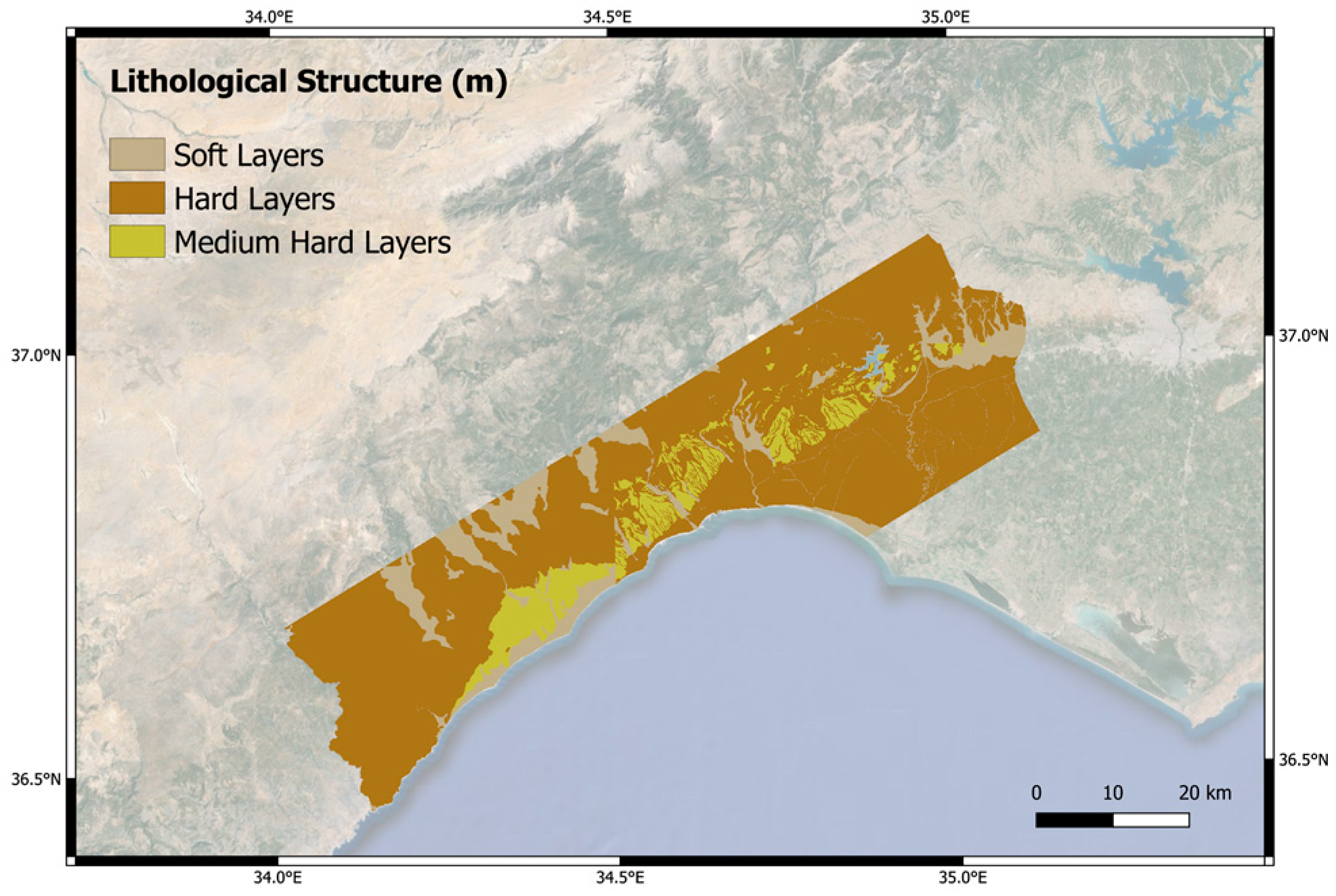
The lithological structure of land is a significant criterion for suitability analysis in urban settlement. It influences construction on the land and plays a crucial role in determining the direction of development [32]. Especially considering the seismic risks in Turkey, including lithology data in the analyses for identifying suitable lands for urban settlement can assist in minimizing potential damage in cities prone to experiencing natural and human-made disasters. Geological data from the General Directorate of Mineral Research and Exploration (MTA) were used to classify the lithological structure of the study area. The study area comprised 24 distinct lithological layers categorized into three groups based on their hardness: soft, medium hard, and hard layers. Soft lithological structures included tuff, gypsum, olistostrome, shale beach, schist-chalk schist, sand dunes, alluvial fan, and melange. Medium hard lithological structures encompassed scree-debris, cones, caliche-terrace, quartzite–quartz system, sandstone–mudstone, and caliche layers. Hard lithological structures consisted of ophiolitic rock, limestone, marble, sandstone–mudstone, travertine, clayey limestone, sandstone–mudstone–limestone, conglomerate sandstone–mudstone, conglomerate limestone, and gravel–sandstone. The classification process utilized the Mohs hardness scale and expert opinions [33]. Figure 6 presents the lithological structure map of the study area.

Subsequently, all criteria maps were resampled to a spatial resolution of 30 m within a Universal Transverse Mercator WGS84 36-coordinate system. A spatial resolution of 30 m was chosen to ensure consistent LULC maps derived from satellite image classification, as discussed in subsequent sub-chapters. These resampled criteria were incorporated into the AHP model to identify suitable locations for urban land use.

2.3. Step II: Generating Urban Land Use Suitability Map via AHP

Saaty [34] introduced AHP to assist decision-makers in handling situations involving numerous conflicting and subjective criteria. Within this method, criteria undergo comparisons utilizing a scale ranging from one to nine. These comparisons categorize criteria as equally important (scaled one), moderately important (scaled three), strongly important (scaled five), very strongly important (scaled seven), extremely important (scaled nine), or with intermediate values (scaled two, four, six, or eight). Subsequently, employing the AHP method, the criteria weights are computed based on the pairwise comparisons matrix. To assess the logical consistency among decision-makers’ opinions, the consistency rate (CR) is computed using Equation (1). This equation incorporates the consistency index (CI) and the random index (RI), with the CI calculated using Equation (2). The CI serves to evaluate the overall inconsistency of the pairwise comparison matrix, aiming for a value below the designated threshold of 0.1. The RI consists of values determined by Saaty and varies based on the number of criteria. In this study, with 13 criteria employed, the RI value is considered to be 1.56. Revision of the comparison matrix is warranted if the inconsistency exceeds this threshold [35].

$$CR=CI/RI$$

(1)

$$CI=\frac{{\lambda }_{max}-n}{n-1}$$

(2)

To assess urban land use suitability via the AHP technique, a survey was conducted to gather decision-makers’ scorings on the selected criteria. A 16-question survey was distributed to 25 participants. The first question required participants to allocate scores to the main criterion groups influencing urban land use suitability analysis, totaling 100 points. Questions 2 to 13 involved scoring the sub-criteria groups based on relative comparisons. Question 14 asked about participants’ areas of expertise, while the final question sought additional expert opinions. Participants included 36.4% urban planners, 27.3% surveying engineers, 18.4% academic staff at universities, and 18% personnel from public institutions.

After determining factor weights using AHP, the subsequent step involved creating a combined suitability map. Here, the weighted linear combination (WLC) method was utilized. This method aims to standardize attribute values for each factor and generate a suitability index by aggregating normalized criteria values. Each alternative’s normalized total weight was computed by multiplying its assigned weight with its normalized value and summing these results. In land suitability studies, factors are termed criteria, with each assigned a weight indicating its importance. Criteria are spatially represented through maps or layers and converted into grid file format for integration within a GIS environment. Equation (3) was employed to combine all criteria using the WLC method.

$${ULSI}_i=\sum _{j=1}^n{W}_j{x}_{ij}$$

(3)

ULSI_i represents the urban land suitability index for a specific cell i, with n denoting the number of criteria. W_j signifies the relative importance weight assigned to criterion j, while x_ij denotes the standardized score of cell i for criterion j [36].

2.4. Step III: Classifying Satellite Imagery for Generating LULC Maps

The third step of this study aimed to classify satellite images, detect changes in the built-up area over the years, and utilize the classification results in urban growth simulation. The methodology for satellite image classification encompassed four main steps: selection of satellite images, classification of satellite images, accuracy assessment of classified images, and analysis of LULC area changes. The selection, classification, and accuracy assessment of satellite images were conducted using the GEE platform. The flowchart summarizing these four steps is depicted in Figure 7.

In this study, Landsat 7 images were used for temporal analysis of LULC area changes. Cloud-free and snow cover-free composite images at five-year intervals (2022, 2017, 2012, and 2007) for the spring and summer months were compiled from atmospherically corrected reflectance (SR) Landsat 7 images with a 30 m spatial resolution on the GEE catalog (Path: 175–174, Row: 35–34). A vector file (.shp) delineating the study area boundaries was uploaded to the GEE platform. The classification analysis utilized the normalized difference vegetation index (NDVI), the normalized difference built-up index (NDBI), and combinations of natural color (RGB) spectral indices, with preliminary findings indicating the highest classification success from the RGB composite images.

The classification study was conducted considering five primary LULC classes. These classes, labeled on the images, included: (1) Built-up areas, encompassing artificial surfaces such as human settlements, developed areas, and concrete-covered areas; (2) agricultural areas, comprising annual and permanent crops, grasslands, and greenhouses; (3) forest areas; (4) water surfaces, including rivers and lakes; and (5) non-agricultural non-forest areas, consisting of areas with sparse vegetation, sandy or rocky terrain.

The classification process aimed to assign each pixel to the appropriate LULC class automatically. However, for supervised image classification, samples of relevant LULC classes need to be provided as training data to the classifier algorithm. Marking selected LULC classes on the images is a prerequisite for training supervised classification algorithms [19]. Therefore, a total of 840 pixels were labeled on images for each year, with 140 pixels randomly distributed for training and 70 pixels for testing per class. These pixels were equally distributed among the five LULC classes. The selected training pixels were used to train the classifier, while the remaining test pixels were used to evaluate the classifier’s performance [37,38]. These pixels were chosen through a visual method enhanced by high-resolution images from Bing and Google Earth, L7 NDVI profiles, false color composites, and local LULC maps. Figure 8 displays the training and test pixels associated with each image composite.

The GEE platform offers built-in functions that allow for the use of classification algorithms such as support vector machines, RF, Naïve Bayes, and decision trees. In this study, the RF classifier algorithm was utilized, which has been widely used in the literature and has been reported to provide higher classification performance [39,40]. The ee.Classifier.smileRandomForest built-in function in GEE was used to generate the classifier model, and hyperparameter tuning was performed. The GridSearchCV method was employed to determine the combination of hyperparameter values of the RF classifier that provide the best performance. This hyperparameter optimization was conducted separately for the classifier model of each image for different years.

The confusion matrix method has been commonly used to evaluate the performance of classifiers by comparing the outputs of classified images with test data. Confusion matrices contain values representing the classified and true class labels. True negative (TN) represents the number of negative pixels correctly classified; true positive (TP) represents the number of positive pixels correctly classified; false positive (FP) represents the number of negative pixels incorrectly classified as positive; and false negative (FN) represents the number of positive pixels incorrectly classified as negative. One of the most frequently used criteria in classification is the confusion matrix, along with derived accuracy metrics such as overall accuracy (OA), producer’s accuracy (PA), and user’s accuracy (UA). The formulas for these accuracy metrics are provided below. OA provides the ratio of correctly predicted pixels to the total number of sample pixels. PA represents the ratio of correctly classified pixels in a specific class to the total number of pixels in the same class. UA represents the ratio of correctly classified pixels in a specific class to the total number of pixels classified as ‘belonging’ to that class. The formulas for these accuracy metrics are provided in Equations (4)–(6). Another performance measure used was the Kappa coefficient, provided in Equation (7). In the context of classification, this coefficient is typically used to evaluate the agreement between what is predicted by a model and the actual class, while also considering the probability of this agreement occurring by chance. A Kappa coefficient of 1 indicates perfect agreement, 0 indicates agreement that could occur by chance, and −1 indicates perfect disagreement. In Equation (7), $p_0$ represents the relative observed agreement in the classifier, and $p_e$ represents the expected probability of chance agreement.

$$OA=(TP+TN)/(TP+FP+TN+FN)$$

(4)

$${PA}_i=\frac{{TP}_i}{{TP}_i+{FN}_i}$$

(5)

$${UA}_i=\frac{{TP}_i}{{TP}_i+{FP}_i}$$

(6)

$$\kappa =\frac{p_0-p_e}{1-p_e}$$

(7)

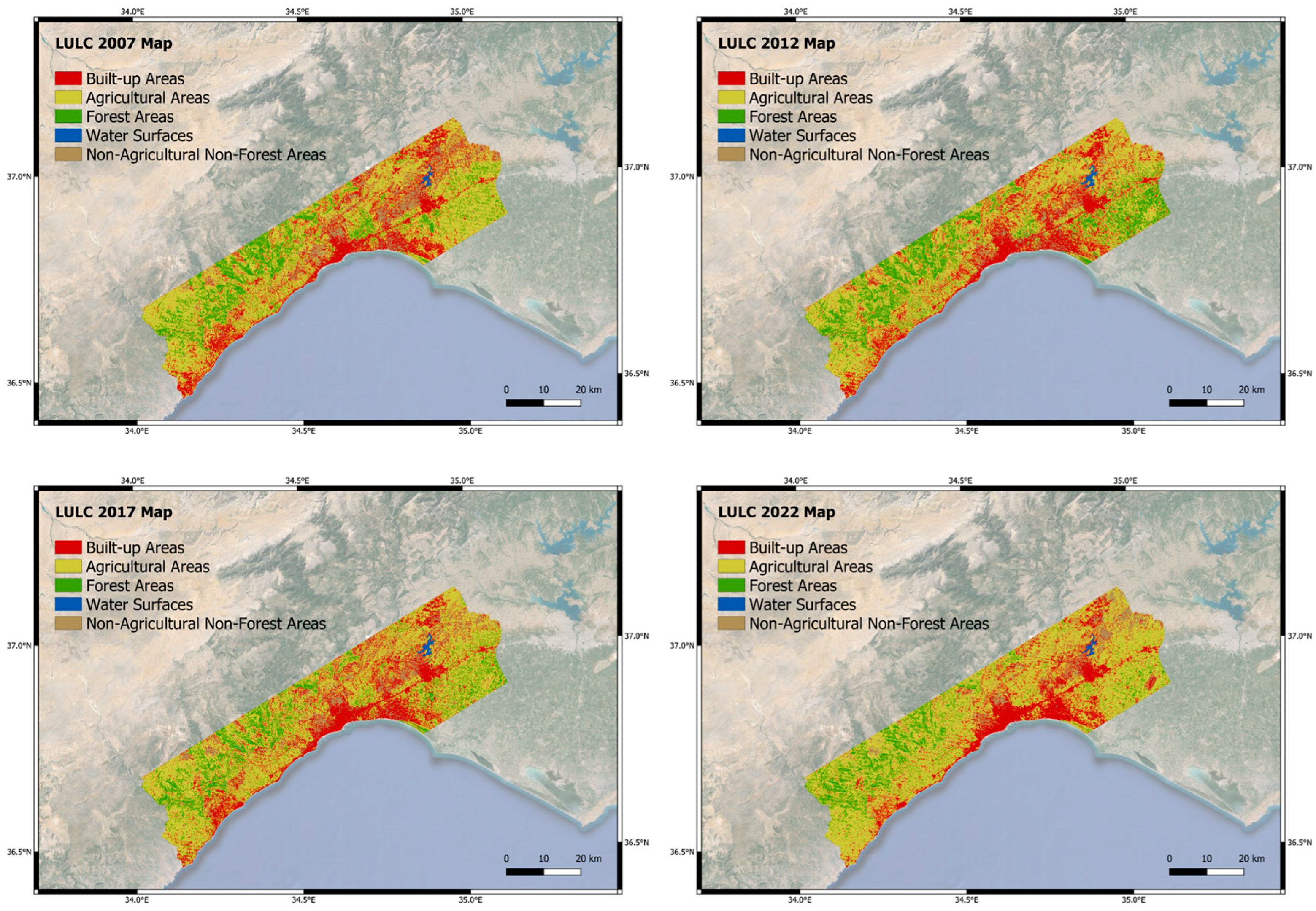
To generate LULC maps for four different years, each comprising five classes, the RF algorithm was employed to run the model that yielded the best prediction results on composite images. Following the classification of all pixels in the images, the resulting images in GEOTIFF format generated on the GEE platform were transferred to the desktop environment and used to create LULC maps for the four years in QGIS 3.34.5 software. These maps facilitated the analysis and mapping of both the LULC distribution for each year and the changes in LULC within each period.

2.5. Step IV: Urban Growth Simulation

Simulation models tracking urban growth have been widely employed over the past two decades, and the predictions derived from these models are utilized to mitigate potential environmental degradation in urban areas during land use planning processes [22,23]. Cellular automata (CA) models, originating from the 1940s work of physicist Stanislaw Ulam and further explored by Von Neumann, offer a powerful tool for deriving urban growth models. They integrate spatial and temporal inputs, allowing for simulation based on predefined rules [41,42]. Furthermore, Markov chain models have also been used to predict LULC changes based on transition probabilities, but sudden changes between LULC states can impact simulation accuracy [43]. Moreover, the SLEUTH model, an open-source urban simulation application developed by Clarke [21], has been widely used and offers scalability and flexibility, but lacks socio-economic data integration [44].

Machine learning (ML) methods have also been leveraged for LULC change analysis and urban growth simulation. Compared to traditional models, ML algorithms offer advantages in handling complex and non-linear relationships in urban dynamics [45]. Among the most commonly used ML methods are logistic regression (LR), support vector machines (SVM) [46], and artificial neural networks (ANN) [47]. LR models, for instance, can express LULC changes mathematically and predict future LULC states based on multiple dependent variables, making them suitable for binary classification problems [48,49]. While each ML method has its strengths and weaknesses, LR was chosen as the primary method for urban growth simulation in this study due to its suitability for binary classification problems and its ability to predict the presence or absence of urban growth based on a set of independent variables. LR assumes that the probability of a cell transitioning to urban use follows a logistic function, with LR coefficients being used to estimate the probability ratios for each independent variable in the model [44]. By representing urban growth outcomes as binary values (Yes or No), LR provides a useful tool for analyzing and predicting urban growth patterns. The probability calculation involves determining how much Y will turn into 1, as shown in Equation (8).

$$P\left(Y=1|X_1,X_2,\dots ,X_n\right)=\frac{1}{1+e^{\alpha +{\sum }_{i=1}^n{\beta }_i{X}_i}}$$

(8)

Here, $P\left(Y=1|X_1,X_2,\dots ,X_n\right)$ is the probability of Y given the values of $X_i(i=\mathrm{1,2},\dots ,n)$. In other words, it is the transformation of non-urban pixel to urban pixel. Additionally, $1-P$ represents the probability of non-existence of urban growth. The regression model is obtained through logistic transformation (Equation (9)).

$$\ln \left(\frac{p}{1-p}\right)=\alpha +{\beta }_1{X}_1+{\beta }_2{X}_2+\cdots +{\beta }_n{X}_n$$

(9)

The coefficients of the independent variables here can be interpreted as factors influencing urban growth, and the probability of urban growth for the entire study area can be calculated iteratively [48].

For the creation of urban growth simulation, past data on LULC classes is required. The input data for urban growth simulation consists of LULC maps from the years 2007, 2012, 2017, and 2022, along with road network data. The road network map, converted from vector to raster format with a 30 m resolution, was compatible with the LULC maps. The reason for using only the road network during simulation is that the analysis of built-up area changes over the years in Mersin indicated that the road network was the most significant factor influencing urbanization. Urban growth simulations were generated for the year 2017 based on the LULC maps from 2007–2012, for 2022 based on the maps from 2012–2017, and for 2027 based on the maps from 2017–2022. The simulation process is illustrated step by step in Figure 9.

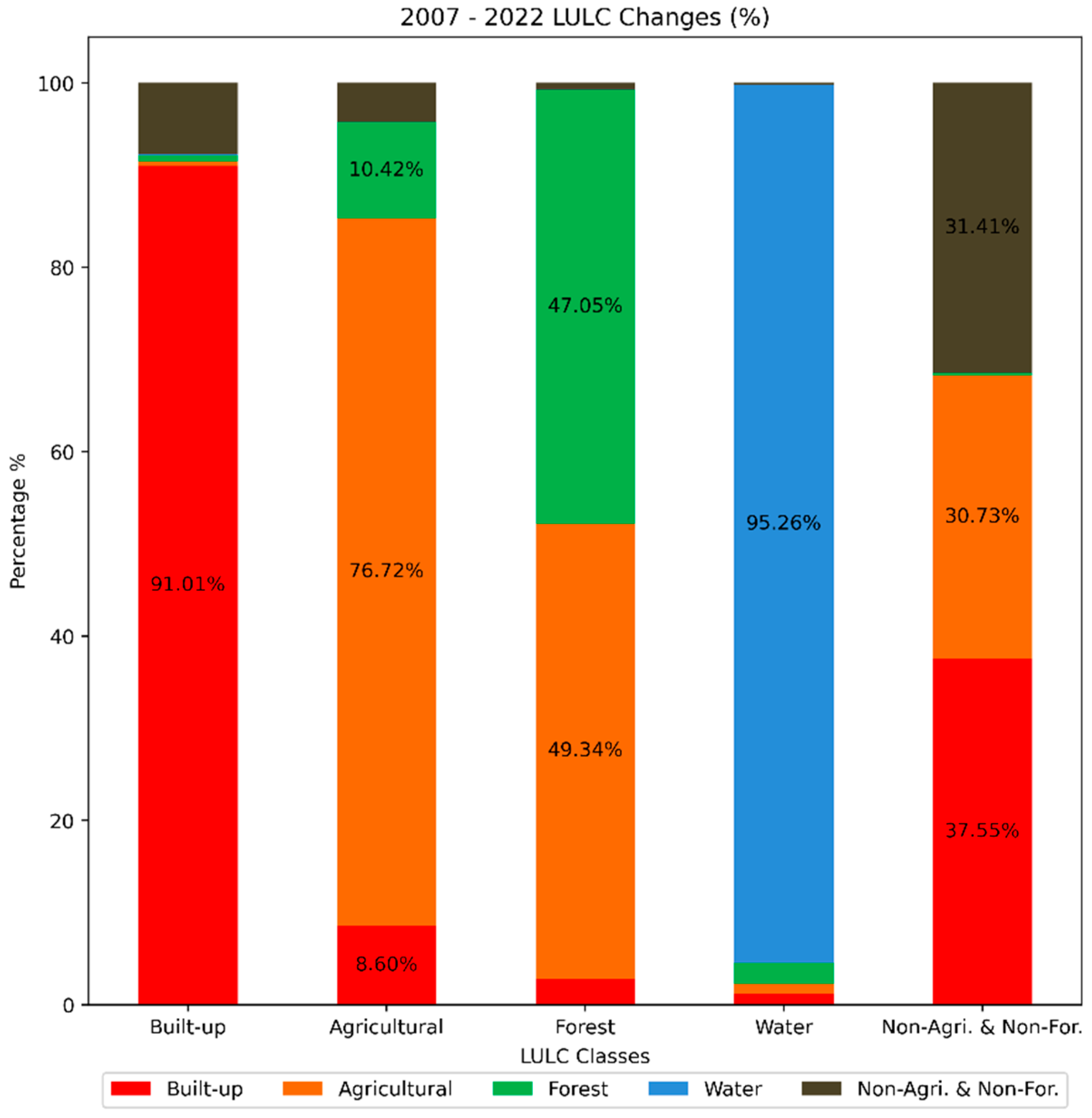
The MOLUSCE package was utilized to generate urban growth simulations. MOLUSCE, an extension used in QGIS 2.0, was developed for examining, modeling, and simulating changes in cities. This extension encompasses methods such as ANN, LR, evidence weights, etc., for urban growth simulations [50]. As indicated before, the LR algorithm was employed for urban growth simulation in this study. In each simulation step, the simulated LULC map for the respective year was compared with the classified LULC area map obtained from classification in terms of pixel consistency, and the simulation performance was evaluated. Additionally, the changes between LULC classes for each five-year period were presented graphically and spatially.

2.6. Step V: Assessment of Future Urban Growth in Accordance with the Urban Land Use Suitability

Following the generation of the simulated LULC map for the year 2027, pixels where urban growth could be observed for the period between 2022 and 2027 were extracted and overlaid with the generated urban land use suitability map. This enabled the assessment of the degree of urban growth in accordance with expected urban land use suitability, and propositions were made based on the quantitative information obtained from this overlay analysis.

3. Results

3.1. Generated Urban Land Use Suitability Map

Based on the criteria utilized, a literature review, and survey results, the binary comparison matrix resulting from the AHP for the suitability analysis of urban land use within the Mersin Metropolitan Area is presented in

Table 2. The binary comparison matrix resulting from the AHP for the suitability analysis of urban land use within the Mersin Metropolitan Area.

Criteria	S	E	A	SC	LULC	RE	TI	ST	BS	RO	P	C	Li
S	1	1/2	3	1/3	1/7	1/5	1/4	2	1/5	1/6	1/2	1/3	1/4
E	2	1	2	1/2	1/9	1/7	1/5	1	1/5	1/4	1/2	1/4	1/3
A	1/3	1/2	1	1/4	1/9	1/8	1/5	1/2	1/5	1/4	1/3	1/4	1/2
SC	3	2	4	1	1/6	1/7	1/5	1/2	1/4	1/5	2	1/2	1/4
LULC	7	9	9	6	1	5	2	8	1	2	5	3	3
RE	5	7	8	7	1/5	1	2	6	1	1	3	2	2
TI	4	5	5	5	1/2	1/2	1	4	1/3	1/4	2	1	1/3
ST	1/2	1	2	2	1/8	1/6	1/4	1	1/5	1/5	1/2	1/4	1/2
BS	5	5	5	4	1	1	3	5	1	1	3	2	1/5
RO	6	4	4	5	1/2	1	4	5	1	1	3	2	1/4
P	2	2	3	1/2	1/5	1/3	1/2	2	1/3	1/3	1	1/2	1/4
C	3	4	4	2	1/3	1/2	1	4	1/2	1/2	2	1	1/2
Li	4	3	2	4	1/3	1/2	3	2	5	4	4	2	1

S: Slope, E: Elevation, A: Aspect, SC: Soil capability, LULC: Land use land cover, RE: Distance to residential areas, TI: Distance to trade and industrial zones, ST: Distance from streams, BS: Distance to bus stops, RO: Distance to roads, P: Distance to port, C: Distance from coastline, Li: Lithological structure.

, while the weights of the criteria and sub-criteria according to their importance are provided in

Table 3. The weights of the criteria and sub-criteria according to their importance.

Criteria	Weight	Sub-Criteria	Weight
Land Use Land Cover	0.173	Built-up Areas	0.280
		Agricultural Areas	0.195
		Forest Areas	0.144
		Non-Agricultural Non-Forest Areas	0.343
		Water Surfaces	0.039
Lithological Structure	0.122	Hard	0.172
		Medium Hard	0.478
		Soft	0.350
Distance to Residential Areas (m)	0.109	0–1000	0.342
		1000–2000	0.272
		2000–3000	0.175
		3000–4000	0.101
		4000–5000	0.061
		>5000	0.048
Distance to Bus Stops (m)	0.107	0–300	0.298
		300–400	0.314
		400–800	0.189
		800–1000	0.096
		1000–2000	0.062
		>2000	0.041
Distance to Roads (m)	0.105	0–150	0.339
		150–1000	0.227
		1000–1500	0.188
		1500–2000	0.100
		2000–2500	0.067
		2500–3000	0.048
		>3000	0.031
Distance to Trade and Industrial Zones (m)	0.071	0–400	0.327
		400–800	0.218
		800–1500	0.200
		1500–2000	0.119
		2000–2500	0.071
		2500–3000	0.038
		>3000	0.027
Distance from Coastline (m)	0.060	0–50	0.319
		50–100	0.258
		100–300	0.162
		300–500	0.125
		500–700	0.068
		700–1000	0.041
		>1000	0.027
Soil Capability	0.034	I–II–III–IV	0.060
		V–VI–VII	0.190
		VIII	0.750
Distance to Port (m)	0.033	0–1000	0.311
		1000–2000	0.214
		2000–3000	0.147
		3000–4000	0.134
		4000–5000	0.085
		5000–6000	0.055
		6000–7000	0.035
		>7000	0.021
Slope (%)	0.021	0–2	0.420
		2–5	0.303
		5–8	0.158
		8–10	0.072
		10	0.048
Distance from Streams (m)	0.021	0–50	0.265
		50–100	0.270
		100–200	0.183
		200–500	0.109
		500–1000	0.068
		1000–1500	0.048
		1500–2000	0.033
		>2000	0.024
Elevation (m)	0.020	0–50	0.417
		50–100	0.248
		100–150	0.176
		150–200	0.098
		>200	0.062
Aspect	0.013	North	0.048
		Northeast	0.048
		Northwest	0.048
		South	0.260
		Southeast	0.140
		Southwest	0.140
		East	0.088
		West	0.088
		Flat	0.140

.

Consistency analysis was conducted on these results to verify whether the binary comparison matrix and the weights of the criteria were consistent. As a result of the calculations, the CR value was obtained as 0.08. Since the CR value was lower than 0.10, it was determined that both the comparison matrix and the criteria weights were at an acceptable level of consistency. According to the calculated criteria weights, land use, lithology, and distance to settlement were identified as the most important criteria. Distance to bus stops and distance to road network were of secondary importance, while proximity to coastal areas, soil suitability, distance to port, slope, distance to rivers, land elevation, and aspect were considered to be less important criteria.

Subsequently, each layer was overlaid to obtain the urban land use suitability index map. In this map, the suitability values of pixels were classified into five categories (very low, low, marginally, moderately, and highly suitable) using the natural breaks method (Figure 10).

When examining this map, it is understood that the suitability decreased towards the outskirts from existing settlements, with the suitability index dropping towards the north of the city. According to the analysis results, it was revealed that areas with very low suitability accounted for the highest proportion in the study area at 30.60% (70,589.34 hectares), areas with a low degree of suitability constituted 27.05% (62,387.19 hectares), while those with a marginal suitability level covered 18.17% (41,922.09 hectares), areas with a moderate suitability level represented 19.50% (44,980.29 hectares), and those identified as high suitability covered 4.68% (10,788.39 hectares) of the total area.

3.2. Generated LULC Maps

The confusion matrices obtained from the performance evaluation on the test data of the composite Landsat 7 images classified using the RF algorithm on the GEE platform, along with the accuracy values, are presented in

Table 4. Confusion matrices for each composite image generated from the test data after training the RF classifier.

		Built-Up Areas	Agricultural Areas	Forest Areas	Water Surfaces	Non-Agricultural and Non-Forest	User’s Accuracy (%)
2022	Built-up Areas	61	3	0	0	6	96
	Agricultural Areas	0	56	14	0	0	80
	Forest Areas	0	0	70	0	0	99
	Water Surfaces	5	4	0	61	0	87
	Non-Agricultural and Non-Forest	3	1	0	0	66	94
	Producer’s Accuracy (%)	96	93	95	97	98
2017	Built-up Areas	56	1	1	0	12	80
	Agricultural Areas	2	58	9	1	0	85
	Forest Areas	0	0	69	1	0	96
	Water Surfaces	3	0	2	65	0	49
	Non-Agricultural and Non-Forest	3	4	0	0	63	90
	Producer’s Accuracy (%)	94	96	96	83	80
2012	Built-up Areas	58	4	0	0	8	83
	Agricultural Areas	0	68	2	0	0	97
	Forest Areas	0	0	69	1	0	99
	Water Surfaces	0	1	0	69	0	99
	Non-Agricultural and Non-Forest	4	0	0	0	66	93
	Producer’s Accuracy (%)	95	98	99	99	96
2007	Built-up Areas	62	1	0	0	7	89
	Agricultural Areas	9	57	3	1	0	81
	Forest Areas	0	3	67	67	0	96
	Water Surfaces	1	2	0	0	0	96
	Non-Agricultural and Non-Forest	6	2	0	0	62	89
	Producer’s Accuracy (%)	93	94	98	98	95

and

Table 5. Kappa coefficients and overall accuracies for the classification of each image composite.

	2007	2012	2017	2022
Kappa	0.89	0.9	0.86	0.88
Overall Accuracy	0.9	0.93	0.88	0.89

, respectively. According to the results, the classification of satellite images for the years 2007, 2012, 2017, and 2022 achieved the desired performance in terms of user accuracy and producer accuracy. Both the class-specific accuracy and overall accuracy values were greater than 0.80, indicating an acceptable level of classification performance. The Kappa coefficients for the classification of images for the years 2007, 2012, 2017, and 2022 were calculated as 0.89, 0.90, 0.86, and 0.88, respectively, while the overall accuracy values were calculated as 0.90, 0.93, 0.88, and 0.89, respectively. The hyperparameters and their values that achieved this performance with the RF classifier are presented in

Table 6. The tuned values for the hyperparameters of the RF classifier.

Year of Image Composite	Number of Decision Trees in the Forest	The Number of Variables per Split	The Maximum Number of Leaf Nodes
2007	100	2	No limit
2012	150	2	No limit
2017	100	2	No limit
2022	100	2	No limit

.

After demonstrating successful performance on the test samples of the composite Landsat 7 images for four different years, the trained RF model was employed for predicting LULC classes for all remaining pixels. Following these prediction processes, a LULC class was assigned to each pixel, thereby obtaining a LULC map from each image. The spatial resolution of these LULC maps was consistent with Landsat 7 images, at 30 m. LULC maps for the four years are depicted in Figure 11.

The proportional distribution of each LULC class in these maps is shown in Figure 12. Upon examination of these LULC maps, it is observed that the proportion of built-up area class to the study area decreased from 21.01% in 2007 to 19.15% in 2022. Agricultural land witnessed an increase over the years, with its proportion rising from 53.40% in 2007 to 60.45% in 2022. Forest area decreased from 15.6% in 2007 to 13.07% in 2022. While the water surface occupied 0.29% of the area in 2007, it increased to 0.31% in 2022, and the area excluding agriculture and forest decreased from 9.71% to 0.31% during the same period.

Separate maps were created to illustrate the changes in LULC classes over the years. These maps contain a legend of 25 classes representing the transition between five different LULC classes and no-change conditions. Figure 13 illustrates the LULC changes between 2007 and 2012 (upper left), the changes between 2012 and 2017 (upper right), and the changes between 2017 and 2022 (lower left). Furthermore, the lower right part provides an overview of LULC changes spanning the entire study period from 2007 to 2022.

Between 2007 and 2022, 91.01% of the built-up areas in the study area remained built-up. In comparison, 76.72% of agricultural areas were preserved, with 8.60% converting to built-up areas, 10.42% to forest areas, 0.05% to water surfaces, and 4.21% to non-agricultural/non-forest areas. Of the forest areas, 47.05% were preserved, with 49.34% converting to agricultural areas, 2.87% to built-up areas, 0.07% to water surfaces, and 0.67% to non-agricultural/non-forest areas. Of the water surface areas, 95.26% were preserved, with 1.22% converting to built-up areas, 1.11% to agricultural areas, 2.18% to forest areas, and 0.23% to non-agricultural/non-forest areas. Of the non-agricultural/non-forest areas, 31.41% were preserved, with 37.55% converting to built-up areas, 30.73% to agricultural areas, 0.27% to forest areas, and 0.04% to water surfaces. A summary of all these changes is provided in Figure 14.

3.3. Urban Growth Simulation Results

As the first step, the simulated LULC map for the year 2017 was obtained using the LR algorithm learned from the LULC maps of 2007 and 2012. The reason for taking this step retrospectively related to the need to calculate the consistency between the simulated LULC map and the LULC map obtained from classification. The overall overlap ratio between these two maps was calculated as 0.72. It was found that there was a difference of 109.35 hectares in built-up areas, 6913.98 hectares in agricultural areas, 10,227.4 hectares in forest areas, 373.5 hectares in water surfaces, and 17,405.5 hectares in non-agricultural/non-forest areas between the simulated LULC map and the classified LULC map. The LULC map for the year 2017 obtained from classification and simulation is shown in Figure 15.

Table 7. Difference in area class distribution between 2017 classification and simulation LULC maps.

	Classified LULC Area (ha)	Simulated LULC Area (ha)	Difference	Difference (%)
Built-up Areas	49,303.26	49,193.91	109.35	0.2%
Agricultural Areas	124,526.34	131,440.32	−6913.98	−5.5%
Forest Areas	35,332.11	45,559.53	−10,227.42	−28.9%
Water Surfaces	1219.05	1592.55	−373.5	−30.6%
Non-Agricultural and Non-Forest	20,296.53	2890.98	17,405.55	85.7%
Sum	230,677.29	230,677.29

presents the distribution difference of LULC classes between these two maps.

Similarly, the LR algorithm trained from the LULC maps of 2012 and 2017 was used to obtain the simulated LULC map for the year 2022. The overall overlap ratio between these two maps was calculated as 0.70. It was found that there was a difference of 657.27 hectares in built-up areas, 5017.23 hectares in agricultural areas, 9918.63 hectares in forest areas, 43.56 hectares in water surfaces, and 5515.11 hectares in non-agricultural/non-forest areas between the simulated LULC map and the classified LULC map. The LULC map for the year 2022 obtained from classification and simulation is shown in Figure 16.

Table 8. Difference in areal class distribution between 2022 classification and simulation LULC maps.

	Classified LULC Area (ha)	Simulated LULC Area (ha)	Difference	Difference (%)
Built-up Areas	44,174.07	43,516.8	657.27	0.014%
Agricultural Areas	139,444.56	144,461.79	−5017.23	−3.5%
Forest Areas	30,141.36	20,222.73	9918.63	32.91%
Water Surfaces	716.58	760.14	−43.56	−6.08%
Non-Agricultural and Non-Forest	16,200.72	21,715.83	−5515.11	−34.04%
Sum	230,677.29	231,677.29

presents the distribution difference of LULC classes between these two maps.

Due to the satisfactory overlap ratio obtained in the step-by-step simulation process, it was deemed appropriate to generate the LULC simulation for the year 2027 using the same technique. The LR algorithm trained from the LULC maps of 2017 and 2022 was used to obtain the simulated LULC map for the year 2027. The objective here was to quantitatively determine how LULC classes will change over the next five years in the Mersin Metropolitan Area and to depict urban expansion. The LULC map for the year 2027 obtained from simulation is shown in Figure 17.

Table 9. Areal distribution of simulated LULC map for the year 2027.

	Total Area (ha)	Distribution (%)
Built-up Areas	36,008.28	15.61
Agricultural Areas	163,440.27	70.85
Forest Areas	21,286.44	9.23
Water Surfaces	588.96	0.26
Non-Agricultural and Non-Forest	9353.34	4.05
Sum	230,677.29	100

presents the area covered by LULC simulation classes in 2027 and the proportion of the study area they occupy.

3.4. Evaluation of Prospective Urban Growth Considering the Suitability of Urban Land Use

With the acquisition of the simulated LULC map for the year 2027, a simulation of urban growth in the Mersin Metropolitan Area has been developed. However, the main research question of this study was to determine the suitability of urban areas where this urban growth will occur. Therefore, it was necessary to overlay the urban land suitability map obtained through the AHP method with the 2027 LULC map in a GIS environment. In this overlaid map, the pixels emerging as newly urbanized areas during the period 2022–2027 were classified in terms of urban land suitability. This map is depicted in Figure 18. In this map, red pixels indicate the least suitable potential urbanization areas, while green pixels indicate the most suitable potential urbanization areas.

Table 10. Urban land use suitability classification of possible development areas for the period 2022–2027.

Suitability	Total Area (ha)
Very Low Suitability	7440.12
Low Suitability	11,938.14
Marginally Suitability	6314.49
Moderately Suitability	7561.44
Highly Suitability	2247.3

displays the spatial distribution of the areas projected for urbanization according to urban land suitability classes for the period 2022–2027 simulation. Accordingly, 2247.3 hectares of potential new urbanization areas demonstrated very suitable suitability for settlement, while 7440.12 hectares exhibited very low suitability.

4. Discussions

Urban growth and economic development are concepts deeply intertwined yet distinct in urban studies, often analyzed through various theoretical frameworks. Urban growth, rooted in urban morphology theories like the concentric zone model by Burgess and the sector model by Hoyt, primarily pertains to the physical expansion of cities, quantifying spatial dimensions such as population increase, infrastructure development, and built-up areas. Economic development, however, is viewed through lenses like modernization theory and dependency theory, focusing on broader aspects of prosperity and well-being within urban areas. While urban growth signifies the physical expansion of a city, economic development assesses improvements in income levels, employment opportunities, and overall economic productivity. This distinction is crucial as urban growth may occur without commensurate economic development, leading to challenges like urban sprawl and infrastructure strain, while robust economic development can transpire in cities without significant physical expansion, fostering sustainable and inclusive growth. Hence, a nuanced understanding of these concepts is crucial for formulating effective urban policies aimed at promoting holistic urban development.

In our study, we aimed to underscore the significance of urban growth in the Mersin Province following a period of substantial economic advancement. The objective was to discern whether the current and prospective urban land use patterns are sufficiently aligned to sustain such economic growth. By investigating the dynamics of urban expansion in tandem with economic development, we sought to shed light on the spatial implications of the province’s prosperity and the extent to which existing land use practices can accommodate future growth trajectories. This analysis holds pivotal importance in informing urban planning strategies and policy interventions geared towards fostering sustainable and resilient urban development in Mersin, ensuring that the province’s economic momentum is supported by a robust and adaptive urban landscape. Therefore, in this study, an analysis of the current situation in Mersin province has been conducted, focusing on the suitability of urban settlements. Additionally, this study attempted to identify future potential urbanization areas using remote sensing and GIS technology.

Mersin, which was a small agricultural and fishing town at the end of the Ottoman period, became an international strategic trade route after a railway line was established with the Adana province, the most important agricultural production center of the Çukurova region in which it is located. These investments prioritized the Adana and Mersin regions as the primary industrial and commercial zones in the first development plans of the period, and the morphology of the developing city was planned and implemented by Hermann Jansen, one of the important urban planners of the period. Planned to be one of the modern cities of the young republic, Mersin, with the completion of the port construction in the 1960s and the industrial investments made in the region, became a growing city. The inadequacy of the existing housing stock became prominent due to the migration it received from rural areas of the country. In order to solve the emerging housing problem, a rapid housing construction policy known as the Build-Sell policy was pursued, and the city’s growth was built on grid-iron formations parallel to the coastline in the western direction. However, these policies could not prevent informal urbanization with fractional parcelization along the belt surrounding the city center, and the formation of a dichotomous urban form became inevitable. After this point, the city’s population growth rate almost doubled, and the city gained an important position both in the country and in the global economy. By the 2000s, the improvement policies in the highway network seen throughout the country found a response with the opening of the Mersin–Adana highway to traffic. Industrial investments supported the urban economy through the port-Free Zone-Railway and Highway transportation network and paved the way for significant investments in the north of the city. While industrial investments found a place in the north of the city, the existing housing stock progressed westward along the coastline for more than 15 km, and the foundation of the city’s current form was shaped with the migration of the neighborhoods on the slopes of the Taurus Mountains, where low-density detached houses were located, to urban life. The growth and transformation of cities became inevitable to meet the housing, health, education, and other needs of the increasing population within the city.

The latest development plan of Turkey includes the agricultural sector under the title “Priority Development Areas”. Under the policies and measures seen in subheadings of Article 405 of this plan, the aim is to ensure the conservation, efficient use, and management of agricultural lands. This study shows that through the classification of satellite images of the current LULC situation and the modeling of future land use and cover through simulation techniques, analyses can be conducted to assist in regulating and monitoring measures that will reduce the pressure of non-agricultural land use on agricultural lands. It will be possible to visually demonstrate in which direction and to what extent the existing/predicted land use and urban sprawl affect the agricultural lands. Examination of the results of these analyses with central and local authorities responsible for formulating land management policies and preparing agricultural land use plans will contribute to the planning of agricultural land use in Turkey in line with sustainable development goals, the preservation of agricultural land while observing conservation and utilization principles, and increasing international branding and competitiveness.

5. Conclusions

This study has demonstrated the efficacy of integrating AHP, GIS, and machine learning techniques to assess urban land suitability and forecast future urban growth in the Mersin Metropolitan Area. Through the generation of an urban land use suitability map and simulation of urban growth scenarios, valuable insights have been gleaned for sustainable urban development planning.

Key findings reveal spatial patterns of land suitability, highlighting areas with varying degrees of suitability for urbanization. The analysis underscores the importance of considering diverse criteria such as topography, accessibility, soil capability, and geology in urban planning processes to ensure informed decision-making. Crucially, the study elucidates the potential impacts of future urban growth on the landscape, facilitating the identification of suitable areas for development while minimizing environmental degradation and preserving natural resources.

GIS and remote sensing technologies play a vital role in urban growth and land use suitability research. These tools enable researchers to collect, analyze, and visualize spatial data, providing valuable information on land use patterns, environmental changes, and demographic trends. By integrating GIS and remote sensing techniques, researchers can conduct comprehensive spatial analyses and identify suitable areas for urban development. These technologies also facilitate the monitoring of urban growth over time and support the formulation of strategic plans for future development.

Despite its contributions, this research has several limitations that should be acknowledged. One limitation is the challenge of data acquisition, particularly in obtaining accurate and comprehensive datasets for analysis. The resolution of available data sources may also affect the scale and scope of the research. Additionally, the exclusion of certain criteria, such as fault line datasets, may limit the comprehensiveness of the analysis. These limitations underscore the need for continued efforts to improve data quality and accessibility in future research endeavors.

Future studies in urban growth and land use suitability research should address the limitations identified in this research and explore new avenues for analysis. Incorporating additional criteria, such as vertical growth considerations and climate change data, can enhance the comprehensiveness of future studies. Moreover, expanding the scope of analysis to include qualitative assessments and societal implications will provide a more holistic understanding of urbanization processes. Continued advancements in GIS and remote sensing technologies will also offer opportunities for conducting more detailed and accurate spatial analyses.