
Exploring the Performance of Continuous-Time Dynamic Link Prediction Algorithms


AIDA, IDLab-ELIS, Department of Engineering and Architecture, Ghent University, 9052 Ghent, Belgium
*
Author to whom correspondence should be addressed.
Appl. Sci. 2024, 14(8), 3516; https://doi.org/10.3390/app14083516
Submission received: 21 March 2024
/
Revised: 11 April 2024
/
Accepted: 17 April 2024
/
Published: 22 April 2024
(This article belongs to the Special Issue Data Mining and Machine Learning in Social Network Analysis)
Abstract
:Dynamic Link Prediction (DLP) addresses the prediction of future links in evolving networks. However, accurately portraying the performance of DLP algorithms poses challenges that might impede progress in the field. Importantly, common evaluation pipelines usually calculate ranking or binary classification metrics, where the scores of observed interactions (positives) are compared with those of randomly generated ones (negatives). However, a single metric is not sufficient to fully capture the differences between DLP algorithms, and is prone to overly optimistic performance evaluation. Instead, an in-depth evaluation should reflect performance variations across different nodes, edges, and time segments. In this work, we contribute tools to perform such a comprehensive evaluation. (1) We propose Birth–Death diagrams, a simple but powerful visualization technique that illustrates the effect of time-based train–test splitting on the difficulty of DLP on a given dataset. (2) We describe an exhaustive taxonomy of negative sampling methods that can be used at evaluation time. (3) We carry out an empirical study of the effect of the different negative sampling strategies. Our comparison between heuristics and state-of-the-art memory-based methods on various real-world datasets confirms a strong effect of using different negative sampling strategies on the test area under the curve (AUC). Moreover, we conduct a visual exploration of the prediction, with additional insights on which different types of errors are prominent over time.
1. Introduction
Many real-world phenomena such as computers networks [1], epidemics [2], neural networks [3], email exchanges [4], and face-to-face interactions [4,5] can be modeled as a set of objects interacting through time. These types of data are commonly represented as a dynamic graph [6], where nodes represent the objects while edges represent pairs of objects that interact through time. While initial attempts at capturing the temporal evolution of networks typically aggregated the interactions into a sequence of static graphs, recent efforts incorporate time continuously, avoiding the loss of some fine-grained temporal information during data preprocessing [6,7]. The resulting types of data are commonly referred to as Continuous-Time Dynamic Graphs (CTDGs) [8]. Modeling and forecasting CTDGs have recently become very active fields of research, as suggested by recent surveys [9,10]. A crucial task of interest is Dynamic Link Prediction (DLP), where the goal is to predict future links from a history of observed ones. This task has gained considerable attention, as seen from recent benchmarks [11], and finds notable applications in recommender systems, influence detection, routing in networks or disease prediction [12,13], to name a few.
Creating a standardized evaluation for Dynamic Link Prediction (DLP) algorithms poses significant challenges [8]. Firstly, the benchmark datasets available vary widely in nature, leading to different domain-specific DLP tasks. Predicting which pair of students will have a face-to-face interaction in the HighSchool dataset at a given time is, for instance, very different from predicting which item a given user will interact with in the Wikipedia dataset. Secondly, the evaluation pipelines differ among methods. This often results in near-perfect performance metrics and contributes to a bias where each paper tends to favor its own proposed approach. Lastly, typical metrics for DLP will compare the score of the actual interactions occurring in the dynamic graph with the scores of interactions that did not happen, obtained through random negative sampling (NS) [14]. As underlined in [8], the procedure used to generate these negative events can have a dramatic impact on DLP performance measures, to the point that some sophisticated methods can often be outperformed by parameter-free heuristics.
As a result, there is a growing awareness that Dynamic Link Prediction performance measures not only depend on the model quality and the challenging nature of the data, but crucially also on the strategy for sampling negative events. Notably, a suggestion proposed by Poursafaei et al. [8] was to generate more challenging negative samples by examining which edges were previously seen or not at test time. These conclusions align with the guidelines proposed by Junuthula et al. [15], who suggest splitting the DLP task into two tasks: predicting previously observed links and predicting previously unobserved links, with each of these tasks coming with their own specific metrics. This same work attributes these challenges to the fact that, while conventional machine learning tasks target independent and identically distributed (iid) data, events, nodes, and node pairs in a (dynamic) graph do not satisfy this property. As a consequence, the prediction performance is likely to exhibit substantial variations depending on the node, edge, or time interval considered.
Despite this growing awareness, central aspects of the DLP task remain ambiguous to this day. Notably, there is a lack of tools for understanding the domain-dependent effect of splitting a history of interaction into a train history and a test history based on a cutoff time. Yet, such an understanding is crucial for designing relevant NS strategies for evaluation. Furthermore, the time evolution of prediction performance tends to be disregarded, despite its significant relevance in real-world applications.
Contributions. In this work, we investigate the open challenges discussed above through visualization and empirical evaluation:
- We introduce the Birth–Death diagram. As illustrated in Figure 1, this simple plot facilitates the visualization and comparison of the lifetimes of nodes and edges (potentially extending to higher-order structures) in a CTDG. Crucially, this visualization tool enables a clear representation of the partitioning of these objects as influenced by the time-based splitting of the history of events. We discuss two key measures derived from these plots, the node and edge surprise indices, quantifying the difficulty of the DLP. We analyze and compare different real-world datasets in terms of these measures.
- We demonstrate the utility of Birth–Death diagrams in the design of more useful negative sampling (NS) strategies for evaluation. By means of these diagrams, we construct a comprehensive taxonomy that categorizes the types of nodes/edges suitable for use as negative instances against which to contrast the scores of positive events. Subsequently, we leverage this taxonomy to develop more targeted NS strategies specifically intended for evaluation. We assess six key NS strategies derived from this approach and analyze the resulting variations in performance.
- Finally, we incorporate time in the evaluation and present a simple visualization method to analyze the time evolution of Dynamic Link Prediction performance of several recent methods and some heuristics.
Our experiments confirm that the performance of methods depend highly on the strategy used for NS. Moreover, the strategy which leads the model to commit more prediction errors (i.e., where the model scores the negative event higher than the positive) varies through time. This observation opens up opportunities for comparing methods empirically by juxtaposing their profile of performance over time. The code is available in open-source at https://github.com/aida-ugent/dlp_exploration.git (accessed on 15 April 2024).
Outline. This paper is divided as follows. In Section 2, we start by discussing related work on dynamic graphs, Dynamic Link Prediction, and strategies for evaluating this task. In Section 3, we formally introduce the Birth–Death diagrams, along with corresponding statistics (the node and edge surprise indices), which are central to assessing the difficulty of the DLP task on a given dataset. In Section 4, we subsequently discuss the evaluation of Dynamic Link Prediction algorithms through NS, and propose a taxonomy of the types of negative samples that can be derived. Finally, in Section 5 and Section 6, we conduct numerical experiments to assess the effect of the different NS strategies, and the evolution of the predictive performance over time.
2. Related Work
Temporal Networks. Temporal networks have been utilized to model extensive systems that comprise entities interacting over time (see Masuda and Lambiotte [7] and Holme and Saramäki [17] for a general introduction). As highlighted by Rozenshtein and Gionis [18], temporal networks have been studied under different terminologies, including dynamic/temporal graphs/networks, depending on the task and the way time is modeled. In particular, some works consider time as discrete [19] and others as continuous [20]. In the present paper, we consider Continuous-Time Dynamic Graphs, as defined in [8,21], and the representation used is the “sequence of interaction model of temporal networks” [18]. The emphasis is on predicting the events on different time intervals, and not on studying emergent properties. Although our focus is on continuous-time graphs, the methodology proposed in this paper applies to both discrete and continuous-time representations.
Visualizing Temporal Networks. Due to the additional complexity introduced by the time dimension, visualizing temporal graphs faces unique challenges, as discussed in recent surveys [22]. As detailed by Linhares et al. [23], the time aspect exacerbates visual clutter issues, which are already common in static network visualization. They propose node activity maps, a method to visualize node activity over time, but do not consider the evaluation of Dynamic Link Prediction as a use case. Temporal edge traffic (TET) and Temporal edge activity (TEA) plots proposed by Poursafaei et al. [8] enable the understanding of the effect of time-based splitting on the edges. However, as these visualizations focus on visualizing the events directly, edges that are exclusively observed in the training set are represented in the region as those observed both in the train and test sets, rendering a visual comparison of these two sets difficult. In contrast, our proposed Birth–Death diagram focuses on directly illustrating the division of nodes and edges into three distinct regions.
Methods for DLP. (Dynamic) Link Prediction is a longstanding problem, and various classes of methods have been proposed to address it. Early efforts focused on using traditional tools from statistics and network science, often borrowing from the existing literature on the modeling of static networks. These include univariate time series models [24,25], similarity-based methods [26], probabilistic generative models [27,28,29,30], and matrix and tensor factorization [31]. Nevertheless, with the success of deep learning and representation learning on static graphs, recent approaches have shifted towards using neural networks, as surveyed by Kazemi et al. [9] and Longa et al. [10]. Notably, memory-based dynamic graph neural networks (DGNNs) such as TGN [21] and DyRep [32], use an encoder–decoder architecture. The encoder maps each node to a time-varying representation in a low-dimensional space, while the decoder allows for calculating the probability of interactions from the latent representations of the nodes. More generally, the idea of learning a vector representation (embedding), either at the node level or the edge level, has been explored in several other papers [33,34,35,36,37,38].
It is important to consider that there is currently a lack of fair and objective comparison between these embedding-based techniques and shallow methods such as the ones previously detailed. Our objective hereby is not to propose a novel method for DLP, but rather to introduce a new performance visualization approach capable of effectively visualizing the DLP task and supporting the performance evaluation of existing methods. Nonetheless, Birth–Death diagrams are particularly pertinent for assessing and diagnosing memory-based DGNNs. Indeed, these models work by maintaining a memory state summarizing the history associated with specific nodes or edges over time. The accuracy and usefulness of this memory state is greatly influenced by the times at which these nodes/edges start (Birth time) and stop (Death time) interacting. We emphasize that our study does not consider negative sampling for training, which has its own challenges [39], but rather for evaluation in Link Prediction.
Challenges in Evaluating DLP Algorithms. Although many methods for static and dynamic Link Prediction have been proposed in the past, the formal definition and evaluation of this task has been subject to much debate and countless refinement over the years. Many evaluation methods have been proposed, including set-based metrics [26], receiver operating characteristic (ROC) curves and associated area under the ROC (AUC–ROC) curve [40,41], and average precision [42]. While the above studies used the time information mainly for splitting the train–test data into a training and a test set, Tylenda et al. [43] presented ways to incorporate the time aspect into a method and evaluation process, demonstrating its positive impact on performance. Subsequently, Junuthula et al. [15] suggested separating the DLP problem into two tasks: the prediction of either recurring edges or newly observed edges. They propose a metric combining AUC–ROC and area under the precision–recall curve to incorporate these two aspects.
In these studies, the impact of negative sampling was often overlooked in the evaluation step. More recently, Poursafaei et al. [8] proposed more challenging negative samples for deep learning-based DLP methods. They introduced three strategies: random, historical, and inductive. In this paper, we extend the literature by proposing a visualization-based method for separating the possible negative samples into categories, with an emphasis on distinctively sampling from overlap and historical edges/nodes. Moreover, we introduce a principle means of scrutinizing the changes in performance over time depending on the negative sampling strategy used for evaluation.
3. Understanding the Effect of Splitting a Dynamic Graph Based on Time
In this section, we provide some background on Continuous-Time Dynamic Graphs (CTDGs). Subsequently, we introduce the notions of Birth and Death time, and the associated Birth–Death diagrams, a visualization tool that allows one to understand the effect of splitting a dynamic graph based on time. Based on this tool, we introduce the node and edge surprise indices as metrics for quantifying the difficulty of predicting future links on a given dynamic graph dataset.
3.1. Background: Continuous-Time Dynamic Graphs
For a set of nodes and maximal time T, a Continuous-Time Dynamic Graph (CTDG) is defined as a stream of events , each representing an interaction of the source node u with the destination node v at timestamp t. We use the term edge to refer to a pair of nodes at an unspecified time. In directed graphs, such an edge in an event is an ordered pair of nodes; in other words, this means that node u sends an interaction to v at time t. Conversely, undirected graphs treat edges as unordered pairs of nodes ; so an interaction means that u and v interacted at time t. In practice, an undirected edge can be uniquely identified by . Further, note that CTDGs allow events to occur at any continuous-valued timestamp and allow multiple events to happen at the same time.
To index the collection of all events in the CTDG, we also introduce some helpful shorthand notations.
We use to represent the set of all events in that involve the node u and to represent the set of events that involve the edge . We also define as the subset of all events in that occur up to a certain time t, i.e., .
Overall, our goal is to better inform the evaluation of Dynamic Link Prediction over CTDGs. We hold off on formally introducing this task until Section 4 and first consider a core decision in any machine learning evaluation: how the data are split up into training and testing data. A typical assumption in dynamic graphs is that we will only need to make predictions about future events. Hence, the train–test split is commonly determined by a cutoff time that partitions the set of events into the train set of past, known events and the test set of ‘future’, unknown events . In what remains of this section, we characterize nodes and edges by whether they are active exclusively in the train set, test set, or in both.
3.2. The Birth and Death of Nodes and Edges
Dynamic graphs dynamically evolve over time. A key motivation for our contributions is that many real CTDG datasets only have nodes and edges that interact within a specific timeframe. For instance, in a social network, a new user may join (represented as a node), or a pair of users (i.e., an edge) may cease interacting entirely at a certain time. To formalize these concepts, we introduce the following definitions.
Definition 1 (Birth time).
For any node or edge , the birth time is defined as the earliest time at which this node or edge is involved in an event in history :
Definition 2 (Death time).
For any node or edge , the death time is defined as the latest time at which this node or edge is involved in an event in history :
Note that, by definition, . These definitions allow us to capture the lifespan of nodes and edges in dynamic graphs, which is crucial for understanding their behavior and evolution over time.
We argue that the Birth and Death times of nodes and edges are highly relevant when splitting up a CTDG’s events into a train set and test set . Such splitting is performed to assess a model’s ability to generalize to unseen data that is encountered in real-world applications, but CTDGs typically see nodes and edges reoccur often. In fact, exploiting recurring patterns is an implicit goal of any machine learning task. Previous work [8,15] has hypothesized that it is far easier for any parametrized model to predict if and when an edge occurs in the test set , if it has already learned from the occurrences of the same edge in the train set . The formal definition of the Birth and Death times helps to elucidate this assumption. For instance, we can state that the occurrence of an edge in the test set will seem more likely to a model if its Birth time was before . Likewise, nodes that were already active in the train set, i.e., they were ‘born’ at time , will be better understood and less surprising than nodes with a Birth time .
Moreover, the extent to which different methods are capable of accurately predicting previously unseen edges in the test set may vary between these different situations. Understanding such differences may be important for choosing the most appropriate method in a particular application.
Therefore, a prudent and useful analysis of (predictions over) a CTDG benefits from partitioning nodes and edges into three categories, which we define here. In all definitions, we denote by the time at which the train–test split is made.
Definition 3 (Historical).
A historical (H) node or edge x only occurs in the train set and never in the test set , i.e.,
Definition 4 (Inductive).
An inductive (I) node or edge x only occurs in the test set and never in the train set , i.e.,
Definition 5 (Overlap).
An overlap (O) node or edge x occurs in both the train set and the test set , i.e.,
3.3. The Birth–Death Diagram
For a given a cutoff time , the Birth and Death times of nodes and edges clearly distinguish whether they are historical, overlap, or inductive. By extension, the distribution of their Birth and Death times characterizes the difficulty of the test set for any cutoff time.
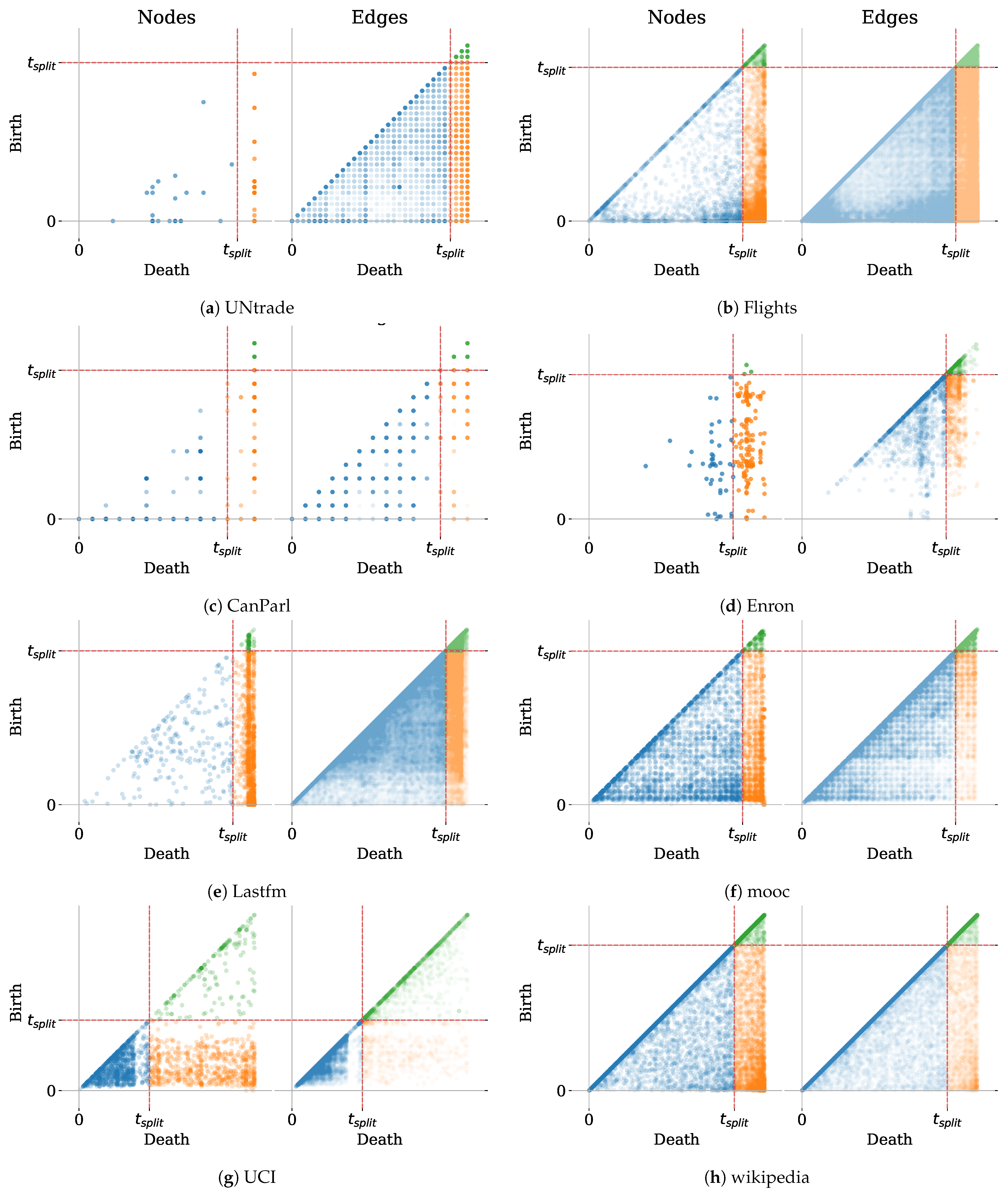
We therefore introduce the Birth–Death diagram: a scatter plot visualization that represents each node or edge by its Birth time (on the y-axis) and Death time (on the x-axis). Figure 1 illustrates the Birth–Death diagram on a dataset of face-to-face interactions among high school students. Moreover, in Figure 2, we plot the Birth–Death diagrams for different CTDG datasets from the benchmark of Poursafaei et al. [8]. We refer the reader to [8] for details about the datasets.
Remark 1.
For all datasets in our illustration, the cutoff time is determined as the -th quantile of the event times, where α is a train–test split ratio set to . In simpler terms, this means that the cutoff time is set to the point in time beyond which 15% of the events occur. Any events that occur before this point in time are included in the training set, while any events that occur after this point in time are included in the test set.
From Figure 2, we can draw some interesting observations, which we discuss here.
Seasonality of Birth and Death Times. The seasonality of lifespan patterns can be observed in both the HighSchool and MOOC datasets as the points corresponding to edges and nodes tend to cluster into squares representing days. The UCI dataset, which describes online interactions among students from April to October 2004, also shows seasonality in the holiday break: there is a white stripe during the holiday break (slightly before ). This seasonality is a crucial property of the Link Prediction task at hand. For instance, in the case of the HighSchool dataset, a possible task can be predicting interactions between students during a specific day, given that we trained a model on the past few days. For these datasets, carefully representing time using techniques such as time encoding [37] can be crucial to achieve good performances.
Short-Lived Nodes and Edges. The high density of points on the diagonal of these diagrams, in particular in the Wikipedia dataset, indicates that most nodes and edges have very short lifespans. As a result, information learned by models about these instances has a higher chance of becoming obsolete after some time. Here, it is crucial that methods take into account time and prioritize active edges/nodes. Conversely, however, some nodes and edges have very long lifetimes in the Wikipedia and Flights datasets (their scatter points are in the lower right), so memorization may work well on these.
“Easy” Datasets. There are some datasets, namely UNtrade, Enron, CanParl, and HighSchool, where most of the nodes are observed at least once in the train set, with only a few nodes starting interactions in the test set. Memorization heuristics such as Preferential Attachment and EdgeBank will constitute strong baselines for these datasets.
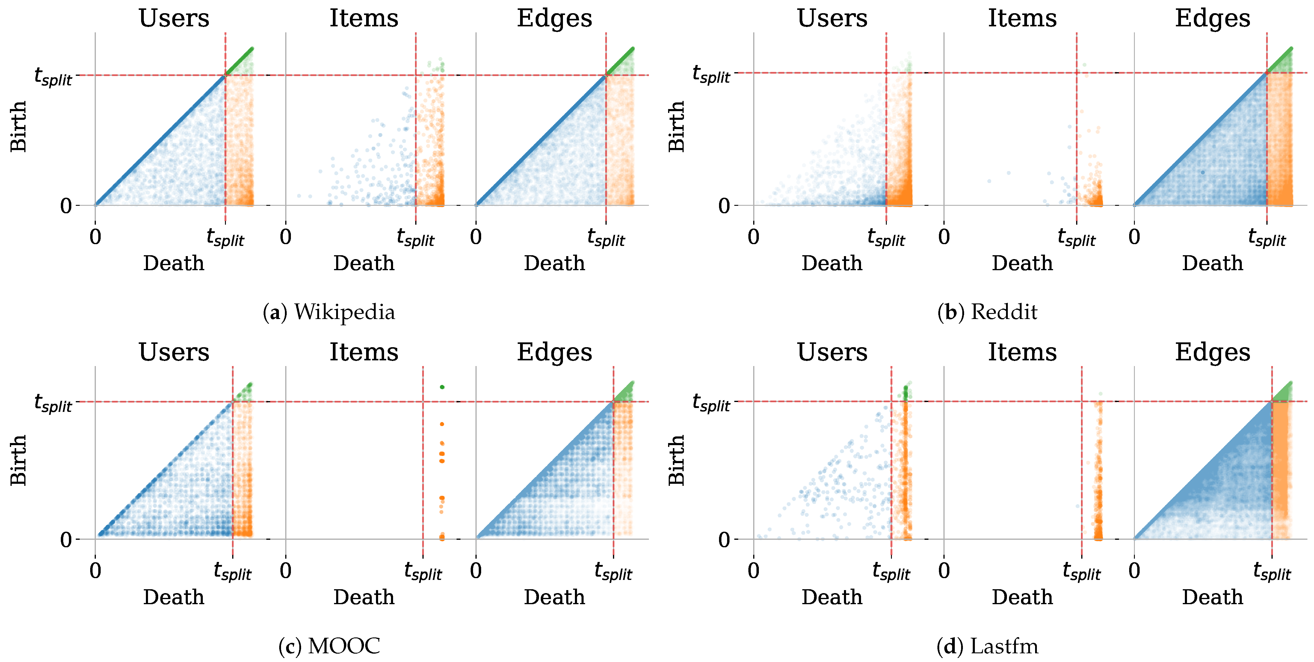
Finally, it is crucial to note that for User–Item graphs, such as Wikipedia, MOOC or Lastfm, the Birth–Death diagram will yield different profiles for the User and Item nodes. We showcase and discuss these differences in Appendix A.
3.4. The Surprise Index
The Birth–Death diagrams suggest that the proportion of overlap and inductive nodes and edges is highly dependent on the cutoff time . We formally assess this proportion through the surprise index, i.e., the proportion of inductive nodes/edges in the test set.
Definition 6 (Surprise Index).
The node/edge surprise index is defined as the proportion of nodes and edges x in the test set (i.e., their Death time ) that only appear in the test set (i.e., their Birth time ). In other words, it is the ratio between the number of inductive (i.e., having a Birth time after ) and the number of inductive or overlap (i.e., having a Death time after ) nodes/edges. Mathematically, considering x to be either the nodes or edges,
Indeed, by definition, the inductive nodes/edges are those whose Birth time is after , while objects which are either inductive or overlap are those whose Death time is after .
Typical ML pipelines will learn from the training data by hinting on recurring patterns (concepts present in the data) and learn to recognize these patterns. The test data may reproduce these patterns to some extent, along with some other signals previously unobserved by the model, which will be reflected in the fact that the predictions will not be imperfect. In the case of the DLP, we dispose of concrete ways of measuring the quantity of information in the test set that will be new for the model. The surprise index is a natural way of measuring that.
In Figure 3, we present the node surprise index against the edge surprise index for various datasets, with train–test splitting ratios ranging from 0.1 to 0.5. By examining these indices, we can observe some interesting properties.
The Surprise Index is Not Necessarily Monotonous with The Size of The Test Set. It may be intuitive to assume that the surprise index increases monotonically with a larger proportion of events included in the test set (i.e., earlier cutoff times ). However, this is not always the case. For instance, in the CanParl dataset, increasing the test ratio from 0.3 to 0.4 actually decreases the edge surprise index, while substantially increasing the node surprise index. A similar non-monotonicity can be observed for the Enron dataset, where increasing the test ratio from 0.3 to 0.4 similarly decreases the edge surprise index. This paradox arises from the fact that the surprise index is a non-decreasing function of the ratio between inductive events (those that occur only in the test set) and overlapping events (those that occur in both the training and test sets). Thus, if adding more events to the test set increases the number of overlapping events faster than it increases the number of inductive events, the surprise index will actually decrease. This observation highlights the importance of carefully selecting cutoff times to ensure that the evaluation setting accurately reflects the difficulty and type of task at hand.
The Edge Surprise Index is Typically Higher than the Node Surprise Index. All datasets evaluated here exhibit curves in the lower right of Figure 2, indicating that the edge surprise index is generally higher than the node surprise index. While this may seem obvious, we stress here that it does not have to be the case. Indeed, what is clear is that if a given node was never observed during training but starts to interact during testing, then it means that the corresponding edge it forms during testing was necessarily never seen during training. As a consequence, there are always at least as many inductive edges as there are inductive nodes. However, the surprise index increases with the ratio between the number of inductive and overlap nodes/edges, and this ratio does not necessarily have to be larger for edges than for nodes. For instance, suppose that four nodes, A, B, C, and D, interact with each other during both the training and test period, resulting in a total of six overlap edges. Now, suppose that a node E starts interacting with A during testing. In this case, the number of inductive nodes and edges are both 1. However, the node surprise index is , while the edge surprise index is , which is smaller. In contrast, if E had started interacting with all four nodes, then we would have an edge surprise of , which would be larger than the node surprise. Another example would be if two nodes E and F would start interacting but only with each other during testing. In this case, the node surprise index would be , while the edge surprise index would be , which is smaller. As such it is in itself an interesting pattern that the edge surprise index is generally higher than the node surprise index in all the considered datasets. Reporting both these indices in practice may give a good first overview of the difficulty of the DLP task at hand.
Domain Dependency. The difference in growth rates between the node and edge surprise indices varies widely across different datasets. For some datasets, increasing the number of events in the test set will increase the proportion of nodes present in the test set that were not observed in the training set. For instance, in the CanParl dataset, increasing the test ratio from 0.1 to 0.3 increases the edge surprise index from 0.15 to around 0.78, while the node surprise index only undergoes a 0.1 increase. This means that while in both cases most of the nodes will already have been observed in the training set, the number of previously unobserved edges will increase significantly. This illustrates the fact that seemingly small changes in the evaluation setting can have a dramatic impact on the difficulty and type of task at hand. The exact values of the node and edge surprise indices, on the datasets from Poursafaei et al. [8], are provided in Table 1.
4. Towards More Targeted Negative Sampling Strategies for Dynamic Link Prediction
The Birth–Death diagrams introduced in Section 3 illustrate the partitioning of nodes and edges into distinct categories: historical, overlap, and inductive. The comparison between a test event and a negative event involving an edge or node from any of these categories presents varying levels of difficulty for the task of discriminating the true event from the negative one. In this section, we operationalize these insights by formally defining Dynamic Link Prediction (DLP) and its connection to negative sampling (NS), before uncovering a taxonomy of the NS strategies targeting different aspects of DLP performance.
4.1. Background on Dynamic Link Prediction
Having thoroughly analyzed the nodes and edges in a CTDG, we now formalize the task of Dynamic Link Prediction (DLP).
Definition 7 (Dynamic Link Prediction).
The Dynamic Link Prediction (DLP) problem is the task of distinguishing positive (true) interactions from interactions that do not occur at the same time t.
For example, the task at hand can be to predict which two people u and v, at the present time t, are most likely to interact in a social network.
Algorithms for DLP. In practice, DLP algorithms are required to output a score that expresses the likelihood of the event given the past history of events up to time t (as any future event would be unavailable at that time). When discussing DLP algorithms, it will then be helpful to also define as shorthand notation for the set of nodes interacting up to time t and for the set of edges. We note that parametric DLP algorithm (e.g., neural networks) will typically output a score that is a function of the past history and of the parameters of the model. Thus, to evaluate the score of a given test event , DLP algorithms are given access to the history up to time t, but are not allowed to update their parameters based on these test events.
Negative Sampling for Evaluation. As already discussed, the goal of DLP algorithms is to accurately score the events , conditioned on the past at time t. Ideally, a perfect model would score any positive event , i.e., an event that actually occurs in history , higher than any negative event , such that , i.e., an event that could have occurred (but did not) at time t. The default strategy would thus be to gather all possible edges and calculate their scores jointly with the positive event at time t. However, computing the scores for all possible edges scales quadratically with the number of nodes. Even for reasonably sized networks with a few thousand nodes, this renders the exhaustive comparison intractable. Consequently, as is the case in Static Link Prediction, it is common to strongly subsample the set of possible negatives. We now formally define this crucial step of the evaluation.
Definition 8 (Negative Sampling).
A negative sampling strategy is a mapping that takes as input a positive event and returns a set of K-associated negative events occurring at the same timestamp t.
Problems with Naive Negative Sampling Strategies. A straightforward NS strategy is to swap the source u and/or destination node v of the positive event with other nodes and/or uniformly at random. Although common, this strategy is naive. The vast majority of possible negatives at time t tends to be unrealistic for various intuitive reasons. For instance, many edges never occur at all in the graph, and many nodes only interact long before or after time t (i.e., they are probably inactive at this time). Such an unrealistic NS strategy may give an unbiased estimate of the exhaustive performance (obtained through a comparison of the positive with all the possible edges). However, including trivial negatives into the comparison will steer the accuracy to a value close to 1, rendering such accuracy rather uninformative. To obtain accuracy estimates which align better with the actual task at hand, it is therefore important to only consider more challenging negatives. In what follows, we will investigate how to do so.
4.2. A Taxonomy of Negative Samples
Given that unrealistic NS leads to an uninformative evaluation of DLP, how might we generate more useful negative samples?
Clearly, this depends on the task at hand. For example, in the Flights dataset, the goal is to predict which destination a plane in a given origin airport will depart to at a given time. In this case, most edges will have been observed already, and it is more interesting to evaluate whether our model can distinguish between the actual origin and destination of the flight and an origin–destination pair that has been previously observed. Therefore, a realistic negative sample could be generated by replacing the actual edges with previously observed edges.
Similarly, in the case of social networks such as email datasets, the goal may be predicting the receiver of a message emitted by a given sender at a certain time. In this case, one may want to specifically sample a negative edge such that the destination node interacts in both the train and test sets. The intuition for such a choice is that models will tend to naturally assign a higher score to events whose nodes have interacted in the train set. Moreover, the fact that these nodes are also present in the test set indicate that they may still be active at the time of the positive interaction, thus making the negative interaction a reasonable candidate.
Here, we aim to contribute NS strategies which can be applied to any dataset or task. Instead of focusing on specific applications, we present a general taxonomy of potential edges that can be used as negative samples. DLP performance can then be appropriately scrutinized for different types of negatives in any application. Considering that machine learning evaluation typically distinguishes performance on the train set from performance on the test set, we make heavy use of our definition of temporal categories in Section 3.2.
Assume any NS strategy starts from a positive event and then ‘corrupts’ it into (realistic) negatives . As discussed previously, the timestamp t is left unchanged, as this is the time at which the prediction is assumed to be made. We can then either corrupt one of the nodes in the event (which we call negative node sampling) or both (which we call negative edge sampling). For both, different strategies can be discerned, as described in the following two definitions.
Definition 9 (Negative Node Sampling).
Negative node sampling (node-NS) takes a positive event and replaces the source node u by or the destination node v by . In both cases, the other node is left the same.
For a given cutoff time , we distinguish six types of negative node samples:
- Historical Source (HS)
- Overlap Source (OS)
- Inductive Source (IS)
- Historical Destination (HD)
- Overlap Destination (OD)
- Inductive Destination (ID)
Remark 2.
In undirected graphs, source and destination sampling are equivalent.
Definition 10 (Negative Edge Sampling).
Negative edge sampling (edge-NS) takes a positive event and replaces the edge by another edge .
For a given cutoff time , we distinguish three types of negative edge samples:
- Historical Edge (HE)
- Overlap Edge (OE)
- Inductive Edge (IE)
These strategies lend themselves to a straightforward visualization interpretation. For instance, in the Birth–Death diagrams (see for instance Figure 2), HE, OE, and IE correspond to sampling the negative edge, respectively, from the set of blue, orange, or green points.
In the rest of this work, we will conduct experiments using the strategies HE, OE, and IE. These strategies enable us to compare the score of a positive event (an action that did happen) with the score of an event that occurred in the dataset but at a different time. Furthermore, we will closely investigate the HD, OD, and ID strategies. These are particularly relevant for evaluating many DLP tasks (e.g., recommendation), where we compare the score of an interaction from a given source (such as a user) to the true destination (an item or another user) with the score of a negative destination that is randomly sampled. The HD, OD, and ID strategies help us understand the impact of choosing a negative destination from different time intervals. This choice can significantly affect the results of an evaluation.
5. Experimental Setup
In the remainder of this paper, we present the extensive experiments conducted in order to validate our evaluation tools, and answer two main questions.
5.1. Datasets
We selected 5 datasets of various sizes from a recent benchmark [8]. Wikipedia is a dataset of edits of Wikipedia pages recorded over one month. Mooc is a dataset of online behavior of students interacting with content (items) on a MOOC platform. Lastfm is a dataset of interaction between users and songs listened by users. Uci is a network of university students communicating over a social network. Enron is a dataset of emails between employees of a company, over a period of three years.
5.2. Methods
In our experiments, we consider 4 different DLP algorithms. The first two methods are simple parameter-free heuristics, which work by memorizing either the nodes or the edges observed in past events. We describe them here, and detail the type of error that these are susceptible to commit:
- Preferential Attachment (PA) assigns a score of 1 to an event if and only if both the nodes have been observed in the past :This method issues a false negative when the true event is such that neither u nor v were ever observed prior to t, and a false positive when the negative event is such that both and were involved in a past event.
- EdgeBank [8] assigns a score of 1 to an event if and only if the edge has been observed in the past :This method yields false negatives whenever the true event is such that the edge was never involved in any event up to time t. It produces false positives whenever the negative event is such that was involved in an event before t.
While simple, these baselines are helpful reference points to assess the performance of more sophisticated methods, as they relate directly to the Birth–Death diagrams presented in Section 3.3. Indeed, one can think of Preferential Attachment and EdgeBank as follows. If we draw a horizontal line at the y coordinate corresponding to the current time t, PA will assign a score of 1 to any event such that both u and v are below the line, i.e., have a Birth time prior to t: and . Similarly, EdgeBank will output a score of 1 to any event such that the edge is represented by a point below the horizontal line with a y coordinate equal to t (i.e., ). On top of these methods, we consider two memory-based dynamic graph representation learning methods, which we briefly introduce below:
- TGN-attn [11] is a DLP algorithm composed of two main modules. A memory module is responsible for maintaining a node-level memory state, encoding the past events at the node level. Using an attention module, the memory states of different nodes are then combined and subsequently used to calculate the probability of the event .
- DyRep [32] has a similar architecture, but specifically uses an attention mechanism on the destination node in order to update the memory given an incoming event.
Remark 3.
In terms of implementation, we use a common approximation to the memory-based methods discussed above. Instead of updating the memory state (set of observed nodes or edges for PA/EdgeBank, node memory states for TGN and DyRep) at every newly observed events, the interactions are consumed by mini batches of 200 events. For each batch, the models successively compute a prediction score for the events in this batch and the associated negative samples, and then update their memory by ingesting the events in that batch.
5.3. Metrics
Binary Classification. In the first experiment, we view DLP as a binary classification task. For each positive event, we draw a negative event at random, following a specific NS strategy. We thus obtain as a result a list of labeled events, where the label indicates whether it is an event that actually occurred or whether it is a negative sample. Considering a given threshold on the prediction scores, a confusion matrix such as the one in Table 2 may then be constructed, measuring the amount of positive/negative events that are scored higher (positive prediction) or lower (negative prediction) than the threshold. By varying the threshold, we can then draw the corresponding receiver operating characteristic (ROC) and compute the associated area under the curve (AUC). Note that this is typically conducted per batch of events, as the prediction scores may not be comparable across batches corresponding to different time spans. The reported AUC is the average of the AUCs obtained on the different batches.
Ranking. In order to assess which negative edge type is more likely to deceive the model at a given time, in a second experiment we consider ranking as a measure of performance. More precisely, we suppose that for each positive event, we assign it a certain number K of negative events, obtained through various NS strategies. Then, we calculate for each of these entries the rank of the positive but also of the associated negatives. Thus, for each event in the test data, we have a list of ranks corresponding to the positive event as well as to different NS strategies, such as NS1, NS2, etc.
In order to obtain a regularly sampled time series, we then partition the time interval time into bins of equal size. For each interval, we calculate the mean average rank (MAR) of all the positives within that interval and perform the same for each NS strategy. As a result, we obtain for each event type (positive, NS strategy 1, NS strategy 2…) a time series of the ranks of the associated events in the different intervals.
For instance, suppose that the first interval contains 4 positive events, to each of which we adjoin 2 negative events (coming from 2 different NS strategies, NS1 and NS2). Now, using the DLP algorithm, we obtain scores for each of the positives and the negatives. Suppose that, as a result, the ranks of the 4 positive events are 1, 3, 2, and 1, the ranks of the negative obtained using NS1 are 2, 1, 3, and 2, and the ranks for NS2 are 3, 2, 1, and 3. Then, for this interval, the MAR for the positive NS1 and NS2 events are , 2, and respectively.
6. Results
In this section, we discuss our experimental results with the aim of answering two research questions. The goal is to assess the impact of the different NS strategies at the aggregate level (Section 6.1) and over time (Section 6.2).
6.1. How Do Performances of DLP Algorithms Vary over Different NS Strategies?
In Figure 4a, we report the AUC scores against three edge-NS: historical edge, overlap edge, and inductive edge negative sampling strategies. Similarly, in Figure 4b, we report AUCs for three destination-NS: historical destination, overlap destination, and inductive destination, as defined in Section 4.2.
In general, the AUC scores are higher when swapping only the destination node, as in Figure 4b. This makes sense when thinking that swapping the destination with random nodes may lead to edges that never happened overall, and thus to negative events that are very unlikely. The overlap edge and overlap destination seem to lead to lower scores in general. Indeed, these strategies yield events that hit a good trade-off between having enough memory about the associated nodes/edges to yield a high score, and being sufficiently novel so that the models do not know yet how to discriminate them from the positive event. In contrast, for historical edges and destination, the involved nodes and edges become relatively obsolete after a certain time, an effect which seems to be picked up by the models.
Starting with the baselines, we note that EdgeBank and Preferential Attachment show very similar performances against historical and overlap edges, with EdgeBank performing worse than random (AUC < 0.5). This can be explained by remembering that, at test time, all the historical edges and overlap edges will have a score of 1. In contrast, the true event may have a score of 1 or 0 depending on whether the associated edges or nodes were previously observed. In that context, the false positive rate is greater than 0 only if the decision threshold is at least 1 (if it is below 1, all the negatives are predicted negative). When the decision threshold reaches the value 1, the number of false positives jumps to the number of negatives (all the negatives will be predicted as positives). In particular, the false positive rate will increase faster than the true positive rate, resulting in an AUC score lower than 0.5.
These figures indicate that NS can be defined such that heuristic baselines outperform neural network-based methods. For instance, in the IE and ID settings, EdgeBank is better than TGN and DyRep on the Lastfm dataset. Moreover, on the Enron dataset, PA outperforms the three other methods in the OD setting, and slightly outperforms TGN in the ID and IE setting. This is counter-intuitive when remembering that PA does not retain any information about the edges active in the past, but only remembers which node was active in the past.
In general, TGN seems to yield a higher score than DyRep. This makes sense considering that DyRep has been shown to be a special case of TGN. However, there are some exceptions, notably in the overlap destination setting where DyRep is better on Lastfm, UCI, and Enron.
6.2. Which Competing Negative Sampling Strategy Misleads the Model More over Time?
In the previous experiment, we observed that using a different NS strategy can dramatically alter the prediction results. However, it is crucial to note that performance evolves over time in a temporal graph. In this section, we demonstrate how distinguishing different NS techniques can help provide a more nuanced insight into the performance of each method over time.
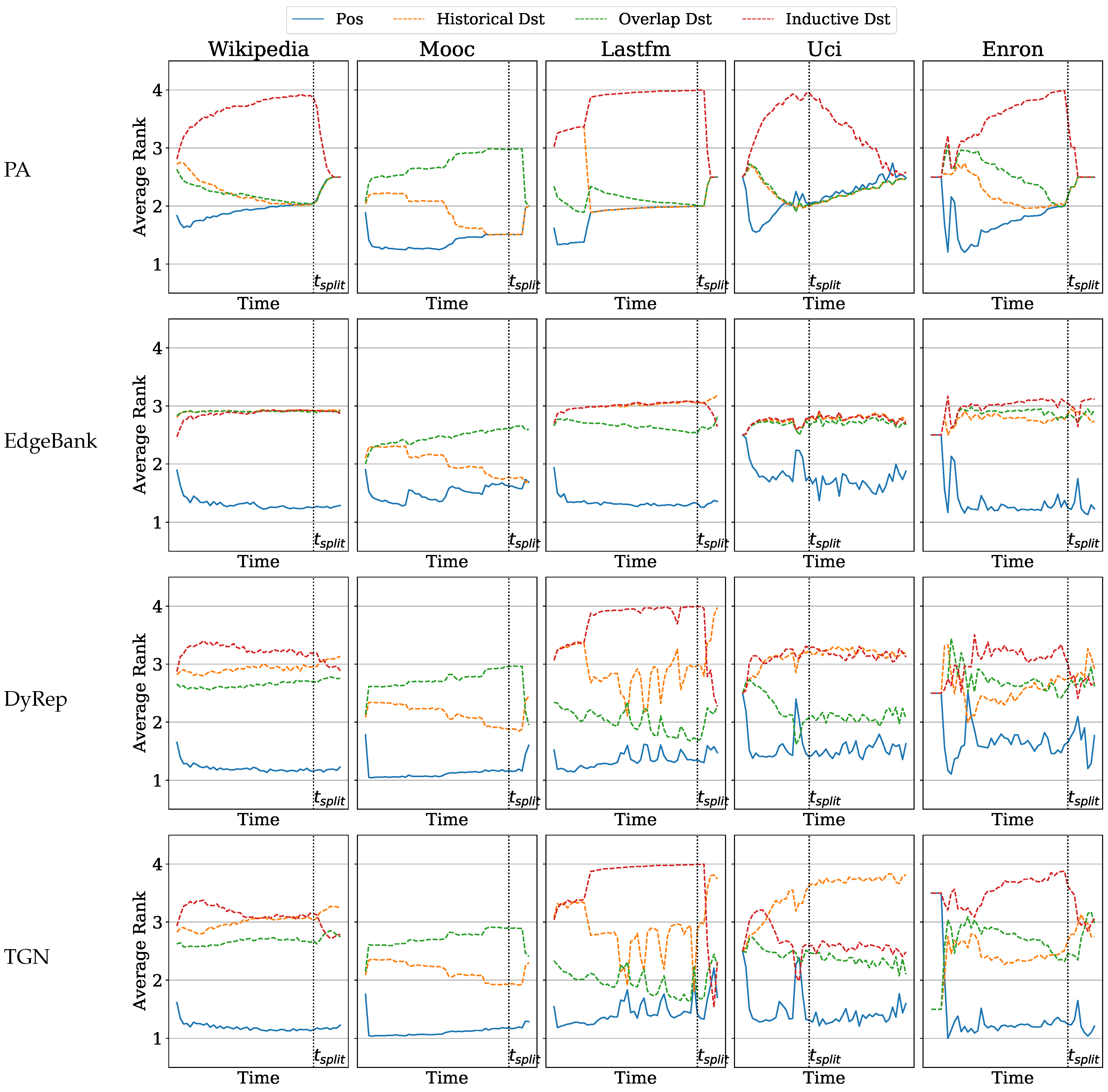
In Figure 5, we observe the performance over time against edge-NS. For all methods and datasets, we note that the rank of the positive events increases over time while the rank of the other edges decreases. Indeed, as memory is filled over time, more events will appear to be likely to occur. In particular, the score of randomly sampled historical and overlap edges will rise in general as compared to the score of the positive event.
A general trend is that the rank of inductive edge/destination NS (green and red lines, respectively) increases on the training period, before dropping on the test set. These types of negative samples will eventually be the ones which will confuse the model during test time, as their rank becomes increasingly closer to the rank of the positive event after . In general, historical and overlap items follow the opposite trend: they become more likely up to , and their rank then starts increasing again either at , or shortly before (notably for historical edges/destinations).
These plots make it clear that the type of error made by the models changes over time. Indeed, while on the train set, inductive edges are likely to be scored low (less likely) since they have not been observed yet; they become much more likely on the test set. Even during the test period, for instance, looking at EdgeBank on the UCI datasets in Figure 5, shortly after , the model will tend to rank the positive events lower than the overlap and historical edges. After some time, however, the inductive edge negative samples will tend to be ranked similarly to the historical and overlap edges.
These visualizations give profound insights on the differences in performance between TGN and DyRep. For instance, on the Lastfm dataset, TGN seems to be more consistent in ranking the inductive destination as high compared with the other destination nodes. However, its overall performance on the test set is not clearly better than DyRep. On the other hand, in Figure 6, the performances on the UCI dataset indicate that, while TGN is clearly able to push historical destinations further than the inductive destination, DyRep tends to assign them similar rankings across the test set.
In both Figure 5 and Figure 6, the examples on the UCI data allow us to visualize the effect of seasonality on the performance. Indeed, for both methods, the rank of the positive event peaks just before the split time. This time corresponds roughly to the lower activity that is also observed in Figure 2g.
To conclude, the results shown in Figure 4, Figure 5 and Figure 6 demonstrate that an overly optimistic AUC may hide a more intricate reality, especially when taking simple baselines as a reference point. While more targeted NS strategies help to identify settings where heuristics outperform proposed heavier models, plotting the performance over time is important to obtain an idea of how a model’s performance will react to domain-specific changes in the data over time.
7. Guidelines for Practitioners
Before concluding this study, we propose the following series of guidelines to practitioners of DLP, with the hope of further improving the evaluation of this task:
- One key conclusion is that evaluating DLP algorithms requires exploring the performance along several dimensions of the data, at the node, edge, and time interval level.
- To do so, as much as possible, a good practice for the use of the DLP algorithm is to enable the saving of the list of scores of each positive event and negative event. Indeed, these scores can be the starting point of in-depth evaluations such as the one conducted in this paper. As suggested in [44], this type of standardized output format is critical in order to easily apply diverse evaluation methods, while minimizing evaluation error.
- Birth–Death diagrams are important tools to understand the effect of time-based train–test splitting on the nodes and edges involved in the graph, and may help in hypothesizing the expected performance of a given method on a given dataset.
- Simple baselines such as EdgeBank and Preferential Attachment baselines are indispensable in order to understand whether the model learns anything non-trivial from the data.
- Finally, visualizing how the prediction performance evolves over time can be crucial in understanding the strengths and weaknesses of DLP algorithms.
8. Conclusions
Recent academic efforts have been dedicated to standardizing Dynamic Link Prediction (DLP) as a machine learning task. The goal is to equip the task with its own evaluation pipelines, baseline methods, and benchmark datasets. However, as a consequence of the high dimensionality of the data and their non-independent, non-identically distributed nature, deriving a single consistent model validation has resulted in numerous challenges.
In this paper, we have explored several key aspects of these challenges. On the one hand, we have investigated the effect of time-based train–test splitting on the set of nodes and edges through novel Birth–Death diagrams, and discussed examples of these visualizations on datasets from diverse domains. Moreover, we have shown how to rely on the proposed Birth–Death diagrams to derive more challenging negative samples, based on the hypothesis that the error depends on the NS strategy. To illustrate the effect of these negative samples, an empirical assessment of the impact of different negative samples on performance was conducted. The relative performance of methods across datasets was compared over time by plotting the prediction ranks as a time series, revealing interesting insights into the failure modes of the different methods.
This work raised several open questions that can be explored in future work. First, our evaluation tools could be used to conduct a more exhaustive comparison of existing heuristics such as the ones introduced in [26], first with simple learning-based approaches such as the ones discussed in Section 2, and then with more recent representation learning methods, with an emphasis on fair comparison. In terms of visualization, the proposed Birth–Death diagrams could be leveraged to visualize higher-order structures such as cliques or triangles, or any repeatedly occurring subgraph that can be uniquely identified.
Author Contributions
Conceptualization, R.R., M.B., T.D.B. and J.L.; Methodology, R.R., M.B. and J.L.; Software, R.R.; Validation, R.R.; Formal analysis, R.R.; Writing—original draft, R.R.; Writing—review & editing, M.B., T.D.B. and J.L. All authors have read and agreed to the published version of the manuscript.
Funding
The research leading to these results has received funding from the Special Research Fund (BOF) of Ghent University (BOF20/IBF/117), from the Flemish Government under the “Onderzoeksprogramma Artificiële Intelligentie (AI) Vlaanderen” programme, and from the FWO (project no. G0F9816N, 3G042220, G073924N).
Institutional Review Board Statement
Not applicable.
Informed Consent Statement
Not applicable.
Data Availability Statement
The original contributions presented in the study are included in the article, further inquiries can be directed to the corresponding author.
Conflicts of Interest
The authors declare no conflicts of interest.
Abbreviations
The following abbreviations are used in this manuscript:
| Notation | Description |
| Set of nodes | |
| T | Maximal time |
| Stream of events | |
| Event representing an interaction of node u with node v at timestamp t | |
| Set of all events in that occur up to time t | |
| Set of nodes involved in interactions up to time t | |
| Set of edges involved in interactions up to time t | |
| Set of events in that involve node u | |
| Set of events in that involve edge | |
| Cutoff time for train–test split | |
| Train set of events occurring up to time | |
| Test set of events occurring after time | |
| Birth time of node or edge x in | |
| Death time of node or edge x in |
Appendix A. Birth–Death Diagrams on User–Item Graphs
The dynamic graphs studied in this paper can be classified into three distinct types:
- Unipartite undirected: For instance, in dynamic graphs of face-to-face interaction such as from the HighSchool dataset, there is only one type of nodes (students), and an interaction between nodes u and v does not have a direction. Contact, SocialEvo, UNvote, and USLegis are examples of such graphs.
- Unipartite directed: For example, in the Enron email dataset, there is only one type of nodes (users involved in mail exchanges). However, the interactions (emails) have an orientation: a given user u sends an email to user v. The datasets UCI, UNtrade, Flights, and Enron are examples of such graphs.
- Bipartite: in this case, there is a clear separation of the nodes into two node types. Typically, in User–Item graphs such as Wikipedia, Lastfm, MOOC, and Reddit, users are always involved in interactions as senders, while items always receive an interaction (a click, a like, a subscription, etc.).
As mentioned in the main body of the paper, Birth–Death diagrams allow us to visualize when nodes and edges start and stop interacting for the first time in a history of events. However, for Bipartite datasets, there is a clear separation between the nodes that will be involved in events as source nodes and those that will appear as destination nodes. For these specific datasets, plotting the Birth and Death time of users and items separately yields extra information. In Figure A1, it can be observed, for instance, that in all datasets, most of the items are overlap nodes in the sense that they are observed in both the train and test sets. In the MOOC dataset, all the items (courses that can be followed by students) are actually observed at least once during the test period; thus, there are no historical destination nodes in that case. For the Lastfm dataset, This is important since for the nodes in the lower right, utilizing the prediction method results in the chance to accumulate a lot of information about them over time. This is in contrast with user nodes, where it can be seen that users more commonly appear and disappear during the training period.
Figure A1.
Birth–Death diagrams on Bipartite User–Item graphs.

Appendix B. Model Architectures and Hyperparameters Used in the Experiments
In the main paper, we compared the performances of TGN-Attn and DyRep with heuristic baselines. We used the implementation provided in the examples of the open-source TGB library https://github.com/shenyangHuang/TGB/tree/main/examples/linkproppred/tgbl-wiki, (accessed on 15 April 2024).
The architecture of the TGN model is as follows:
- The message function is the identification function (the same as in the original paper [21]).
- The aggregation function is the last message aggregator (we keep for each node only the last message received from the batch).
- The memory updater is a GRU.
- The embedding module is a temporal graph attention layer. Its purpose is to integrate both the network’s connectivity information and temporal data, ensuring that embeddings remain current by combining the memory state with the most recent network information.
- The edge-level decoder (i.e., Link Predictor) is a two-layer MLP with 100 hidden units and ReLU activation.
The DyRep model implemented in the library is very similar to the TGN architecture, with two main differences:
- The memory updater is a simple RNN.
- The embedding module is the identity: the memory is used directly for prediction. Note that this makes the model vulnerable to the memory staleness problem.
- However, the messages function is calculated using a graph attention module on the destination node.
Hyperparameters. As the goal of our study is not to maximize the performance but to compare it across negative sampling strategies, we used the default hyperparameter values for both TGN-Attn and DyRep. Thus, the memory, time encoding, and embedding dimensions are all set to 100. We use the Adam Optimizer [45] with a learning rate of and a weight decay of . To prevent overfitting, we use early stopping on the validation of AUC: we stop the training if there has been no improvement in the AUC of more than in the last 20 epochs.
References
- Yoon, M.; Hooi, B.; Shin, K.; Faloutsos, C. Fast and Accurate Anomaly Detection in Dynamic Graphs with a Two-Pronged Approach. In Proceedings of the 25th ACM SIGKDD International Conference on Knowledge Discovery & Data Mining, Anchorage, AK, USA, 4–8 August 2019; pp. 647–657. [Google Scholar] [CrossRef]
- Machens, A.; Gesualdo, F.; Rizzo, C.; Tozzi, A.E.; Barrat, A.; Cattuto, C. An Infectious Disease Model on Empirical Networks of Human Contact: Bridging the Gap between Dynamic Network Data and Contact Matrices. BMC Infect. Dis. 2013, 13, 185. [Google Scholar] [CrossRef] [PubMed]
- Cadena, J.; Sales, A.P.; Lam, D.; Enright, H.A.; Wheeler, E.K.; Fischer, N.O. Modeling the Temporal Network Dynamics of Neuronal Cultures. PLoS Comput. Biol. 2020, 16, e1007834. [Google Scholar] [CrossRef] [PubMed]
- Klimt, B.; Yang, Y. The Enron Corpus: A New Dataset for Email Classification Research. In Machine Learning: ECML 2004; Boulicaut, J.F., Esposito, F., Giannotti, F., Pedreschi, D., Eds.; Springer: Berlin/Heidelberg, Germany, 2004; Lecture Notes in Computer Science; pp. 217–226. [Google Scholar] [CrossRef]
- Eagle, N.; Pentland, A. Reality Mining: Sensing Complex Social Systems. Pers. Ubiquitous Comput. 2006, 10, 255–268. [Google Scholar] [CrossRef]
- Holme, P.; Saramäki, J. Temporal Networks as a Modeling Framework. arXiv 2021, arXiv:2103.13586. [Google Scholar] [CrossRef]
- Masuda, N.; Lambiotte, R. A Guide to Temporal Networks; Complexity Science, World Scientific Publishing: Singapore, 2016. [Google Scholar]
- Poursafaei, F.; Huang, A.; Pelrine, K.; Rabbany, R. Towards Better Evaluation for Dynamic Link Prediction. In Proceedings of the Thirty-Sixth Conference on Neural Information Processing Systems Datasets and Benchmarks track, New Orleans, LA, USA, 10–16 December 2023. [Google Scholar]
- Kazemi, S.M.; Goel, R.; Jain, K.; Kobyzev, I.; Sethi, A.; Forsyth, P.; Poupart, P. Representation Learning for Dynamic Graphs: A Survey. J. Mach. Learn. Res. 2020, 21, 2648–2720. [Google Scholar]
- Longa, A.; Lachi, V.; Santin, G.; Bianchini, M.; Lepri, B.; Lio, P.; Scarselli, F.; Passerini, A. Graph Neural Networks for Temporal Graphs: State of the Art, Open Challenges, and Opportunities. arXiv 2023, arXiv:2302.01018. [Google Scholar]
- Huang, S.; Poursafaei, F.; Danovitch, J.; Fey, M.; Hu, W.; Rossi, E.; Leskovec, J.; Bronstein, M.; Rabusseau, G.; Rabbany, R. Temporal Graph Benchmark for Machine Learning on Temporal Graphs. arXiv 2023, arXiv:2307.01026. [Google Scholar] [CrossRef]
- Srinivas, V.; Mitra, P.; Srinivas, V.; Mitra, P. Applications of Link Prediction. In Link Prediction in Social Networks; Springer: Cham, Switzerland, 2016; pp. 57–61. [Google Scholar] [CrossRef]
- Kumar, A.; Singh, S.S.; Singh, K.; Biswas, B. Link Prediction Techniques, Applications, and Performance: A Survey. Phys. A Stat. Mech. Its Appl. 2020, 553, 124289. [Google Scholar] [CrossRef]
- Mikolov, T.; Chen, K.; Corrado, G.; Dean, J. Efficient Estimation of Word Representations in Vector Space. arXiv 2013, arXiv:1301.3781. [Google Scholar] [CrossRef]
- Junuthula, R.R.; Xu, K.S.; Devabhaktuni, V.K. Evaluating Link Prediction Accuracy in Dynamic Networks with Added and Removed Edges. In Proceedings of the 2016 IEEE International Conferences on Big Data and Cloud Computing (BDCloud), Social Computing and Networking (SocialCom), Sustainable Computing and Communications (SustainCom) (BDCloud-SocialCom-SustainCom), Atlanta, GA, USA, 8–10 October 2016; pp. 377–384. [Google Scholar] [CrossRef]
- Fournet, J.; Barrat, A. Contact Patterns among High School Students. PLoS ONE 2014, 9, e107878. [Google Scholar] [CrossRef]
- Holme, P.; Saramäki, J. Temporal Networks. Phys. Rep. 2012, 519, 97–125. [Google Scholar] [CrossRef]
- Rozenshtein, P.; Gionis, A. Mining Temporal Networks. In Proceedings of the 25th ACM SIGKDD International Conference on Knowledge Discovery & Data Mining, New York, NY, USA, 25 July 2019; KDD ’19. pp. 3225–3226. [Google Scholar] [CrossRef]
- He, J.; Chen, D. A fast algorithm for community detection in temporal network. Phys. A Stat. Mech. Its Appl. 2015, 429, 87–94. [Google Scholar] [CrossRef]
- Latapy, M.; Viard, T.; Magnien, C. Stream Graphs and Link Streams for the Modeling of Interactions over Time. Soc. Netw. Anal. Min. 2018, 8, 61. [Google Scholar] [CrossRef]
- Rossi, E.; Chamberlain, B.; Frasca, F.; Eynard, D.; Monti, F.; Bronstein, M. Temporal Graph Networks for Deep Learning on Dynamic Graphs. arXiv 2020, arXiv:2006.10637. [Google Scholar]
- Beck, F.; Burch, M.; Diehl, S.; Weiskopf, D. A Taxonomy and Survey of Dynamic Graph Visualization. Comput. Graph. Forum 2017, 36, 133–159. [Google Scholar] [CrossRef]
- Linhares, C.D.G.; Travençolo, B.A.N.; Paiva, J.G.S.; Rocha, L.E.C. DyNetVis: A System for Visualization of Dynamic Networks. In Proceedings of the Symposium on Applied Computing, Marrakech, Morocco, 3–7 April 2017; SAC ’17. pp. 187–194. [Google Scholar]
- Güneş, İ.; Gündüz-Öğüdücü, Ş.; Çataltepe, Z. Link Prediction Using Time Series of Neighborhood-Based Node Similarity Scores. Data Min. Knowl. Discov. 2016, 30, 147–180. [Google Scholar] [CrossRef]
- Huang, Z.; Lin, D.K.J. The Time-Series Link Prediction Problem with Applications in Communication Surveillance. INFORMS J. Comput. 2009, 21, 286–303. [Google Scholar] [CrossRef]
- Liben-Nowell, D.; Kleinberg, J. The link-prediction problem for social networks. J. Am. Soc. Inf. Sci. Technol. 2007, 58, 1019–1031. [Google Scholar] [CrossRef]
- Foulds, J.R.; DuBois, C.; Asuncion, A.U.; Butts, C.T.; Smyth, P. A Dynamic Relational Infinite Feature Model for Longitudinal Social Networks. In Proceedings of the International Conference on Artificial Intelligence and Statistics, Fort Lauderdale, FL, USA, 11–13 April 2011. [Google Scholar]
- Heaukulani, C.; Ghahramani, Z. Dynamic Probabilistic Models for Latent Feature Propagation in Social Networks. In Proceedings of the 30th International Conference on Machine Learning, Atlanta, GA, USA, 16–21 June 2013; pp. 275–283. [Google Scholar]
- Xu, K.S. Stochastic Block Transition Models for Dynamic Networks. arXiv 2015, arXiv:1411.5404. [Google Scholar] [CrossRef]
- Kim, M.; Leskovec, J. Nonparametric Multi-group Membership Model for Dynamic Networks. In Proceedings of the Advances in Neural Information Processing Systems, Lake Tahoe, NV, USA, 5–8 December 2013; Volume 26. [Google Scholar]
- Dunlavy, D.M.; Kolda, T.G.; Acar, E. Temporal Link Prediction Using Matrix and Tensor Factorizations. ACM Trans. Knowl. Discov. Data 2011, 5, 1–27. [Google Scholar] [CrossRef]
- Trivedi, R.; Farajtabar, M.; Biswal, P.; Zha, H. DyRep: Learning Representations over Dynamic Graphs. In Proceedings of the International Conference on Learning Representations, New Orleans, LA, USA, 6–9 May 2019. [Google Scholar]
- Cong, W.; Zhang, S.; Kang, J.; Yuan, B.; Wu, H.; Zhou, X.; Tong, H.; Mahdavi, M. Do We Really Need Complicated Model Architectures for Temporal Networks? In Proceedings of the The Eleventh International Conference on Learning Representations, Kigali, Rwanda, 1–5 May 2023; ICLR: Vienna, Austria, 2023. Available online: https://openreview.net/forum?id=ayPPc0SyLv1 (accessed on 15 April 2024).
- Luo, Y.; Li, P. Neighborhood-Aware Scalable Temporal Network Representation Learning. In Proceedings of the First Learning on Graphs Conference, Virtual, 9–12 December 2022; Volume 198, pp. 1:1–1:18. [Google Scholar]
- Wang, Y.; Chang, Y.Y.; Liu, Y.; Leskovec, J.; Li, P. Inductive Representation Learning in Temporal Networks via Causal Anonymous Walks. In Proceedings of the International Conference on Learning Representations, Virtual, 3–7 May 2021; ICLR: Vienna, Austria, 2021. Available online: https://openreview.net/forum?id=KYPz4YsCPj (accessed on 15 April 2024).
- Wang, L.; Chang, X.; Li, S.; Chu, Y.; Li, H.; Zhang, W.; He, X.; Song, L.; Zhou, J.; Yang, H. TCL: Transformer-based Dynamic Graph Modelling via Contrastive Learning. arXiv 2021, arXiv:2105.07944. [Google Scholar] [CrossRef]
- Xu, D.; Ruan, C.; Korpeoglu, E.; Kumar, S.; Achan, K. Inductive Representation Learning on Temporal Graphs. arXiv 2020, arXiv:2002.07962. [Google Scholar] [CrossRef]
- Yu, L.; Sun, L.; Du, B.; Lv, W. Towards Better Dynamic Graph Learning: New Architecture and Unified Library. In Proceedings of the Thirty-Seventh Conference on Neural Information Processing Systems, New Orleans, LA, USA, 10–16 December 2023. [Google Scholar]
- Daniluk, M.; Dąbrowski, J. Temporal graph models fail to capture global temporal dynamics. arXiv 2023, arXiv:2309.15730. [Google Scholar] [CrossRef]
- Lu, L.; Zhou, T. Link Prediction in Complex Networks A Survey. Phys. A Stat. Mech. Its Appl. 2011, 390, 1150–1170. [Google Scholar] [CrossRef]
- Lichtenwalter, R.; Lussier, J.; Chawla, N. New Perspectives and Methods in Link Prediction. In Proceedings of the ACM SIGKDD International Conference on Knowledge Discovery and Data Mining, Washington, DC, USA, 25–28 July 2010; pp. 243–252. [Google Scholar]
- Yang, Y.; Lichtenwalter, R.N.; Chawla, N.V. Evaluating Link Prediction Methods. Knowl. Inf. Syst. 2015, 45, 751–782. [Google Scholar] [CrossRef]
- Tylenda, T.; Angelova, R.; Bedathur, S. Towards Time-Aware Link Prediction in Evolving Social Networks. In Proceedings of the 3rd Workshop on Social Network Mining and Analysis, Paris, France, 28 June 2009; SNA-KDD ’09. pp. 1–10. [Google Scholar] [CrossRef]
- Mara, A.; Lijffijt, J.; De Bie, T. EvalNE: A Framework for Network Embedding Evaluation. SoftwareX 2022, 17. [Google Scholar] [CrossRef]
- Kingma, D.P.; Ba, J. Adam: A Method for Stochastic Optimization. arXiv 2017, arXiv:1412.6980. [Google Scholar] [CrossRef]
Figure 1.
A Birth–Death diagram on a recording of face-to-face interactions among high school students over 9 days [16]. The y and x coordinates for each node/edge represent their first (Birth) and last (Death) interaction time, respectively. Given a cutoff time , while the history of interaction is divided into a train or a test set, the nodes and edges are partitioned into three categories: historical, overlap, and inductive. The surprise index is the ratio .

Figure 2.
Birth–Death diagrams for nodes and edges in datasets from the dynamic graph benchmark from Poursafaei et al. [8]. The datasets are split into train and test sets containing 85% and 15% of the events, respectively.
Figure 2.
Birth–Death diagrams for nodes and edges in datasets from the dynamic graph benchmark from Poursafaei et al. [8]. The datasets are split into train and test sets containing 85% and 15% of the events, respectively.

Figure 3.
Changing the test split ratio linearly from 0.1 to 0.5 changes the node and edge surprise indices differently depending on the dataset. The typical test split ratio of 0.15 is marked as “*” on the lines.
Figure 3.
Changing the test split ratio linearly from 0.1 to 0.5 changes the node and edge surprise indices differently depending on the dataset. The typical test split ratio of 0.15 is marked as “*” on the lines.

Figure 4.
Test AUC results obtained by comparing the scores of the positive events with the scores of the negative events, sampled using specific strategies. For DyRep and TGN, we retrained the models with 5 different seeds and report the mean and the standard deviation of the resulting AUCs. (a) Test AUC results employing various edge negative sampling strategies: historical edge (HE), overlap edge (OE), and inductive edge (IE). These strategies involve sampling negative edges (u’,v’) from sets corresponding to edges exclusively present during training, those present during both training and testing, and those exclusively present during testing, respectively. (b) Test AUC results employing various destination negative sampling strategies: historical destination (HD), overlap destination (OD), and inductive destination (ID). These strategies swap the destination node with one present during training, both training and testing, or exclusively during testing.

Figure 5.
MAR of each method over time. The positive event “Pos” is ranked against negative events resulting from different negative edge sampling strategies as defined in Section 4.2: historical edge, overlap edge, and inductive edge.
Figure 5.
MAR of each method over time. The positive event “Pos” is ranked against negative events resulting from different negative edge sampling strategies as defined in Section 4.2: historical edge, overlap edge, and inductive edge.

Figure 6.
MAR of each method over time. The positive event “Pos” is ranked against negative events resulting from different negative destination sampling strategies as defined in Section 4.2: historical destination, overlap destination, inductive destination.
Figure 6.
MAR of each method over time. The positive event “Pos” is ranked against negative events resulting from different negative destination sampling strategies as defined in Section 4.2: historical destination, overlap destination, inductive destination.


Table 1.
Dataset statistics, including the node and edge surprise indices, for a test ratio of 15%. For most datasets, the nodes are mostly all observed during training, hence a relatively low node surprise index. The edge surprise is higher however, since many edges that interact in the test set were never observed in the test set.
| Events | Nodes | Edges | |||||||||
|---|---|---|---|---|---|---|---|---|---|---|---|
| Total | Historical | Overlap | Inductive | Surprise | Total | Historical | Overlap | Inductive | Surprise | ||
| UCI | 59,835 | 1899 | 1052 | 681 | 166 | 0.196 | 20,296 | 17,069 | 657 | 2570 | 0.796 |
| HighSchool | 45,047 | 180 | 18 | 160 | 2 | 0.012 | 2239 | 1577 | 445 | 217 | 0.328 |
| Wikipedia | 157,474 | 9227 | 5663 | 2648 | 916 | 0.257 | 18,257 | 13,667 | 2046 | 2544 | 0.554 |
| Enron | 25,235 | 184 | 43 | 138 | 3 | 0.021 | 3125 | 1914 | 724 | 487 | 0.402 |
| USLegis | 60,396 | 225 | 112 | 101 | 12 | 0.106 | 26,423 | 18,884 | 5857 | 1682 | 0.223 |
| UNvote | 1,035,742 | 201 | 7 | 194 | 0 | 0.000 | 31,516 | 4487 | 26,583 | 446 | 0.017 |
| UNtrade | 507,497 | 255 | 27 | 228 | 0 | 0.000 | 36,182 | 10,595 | 24,347 | 1240 | 0.048 |
| SocialEvo | 2,099,519 | 74 | 12 | 62 | 0 | 0.000 | 4486 | 2609 | 1827 | 50 | 0.027 |
| MOOC | 411,749 | 7144 | 4732 | 2185 | 227 | 0.094 | 178,443 | 147,612 | 6628 | 24,203 | 0.785 |
| Flights | 1,927,145 | 13,169 | 2182 | 10,698 | 289 | 0.026 | 395,072 | 264,189 | 85,369 | 45,514 | 0.348 |
| 672,447 | 10,984 | 1369 | 9578 | 37 | 0.004 | 78,516 | 53,589 | 17,933 | 6994 | 0.281 | |
| Lastfm | 1,293,103 | 1980 | 227 | 1681 | 72 | 0.041 | 154,993 | 106,038 | 30,883 | 18,072 | 0.369 |
| CanParl | 74,478 | 734 | 384 | 340 | 10 | 0.029 | 51,331 | 38,401 | 7432 | 5498 | 0.425 |
Table 2.
Confusion matrix.
| Predicted/Actual | Actual Positive | Actual Negative |
|---|---|---|
| Predicted Positive | True Positive (TP) | False Positive (FP) |
| Predicted Negative | False Negative (FN) | True Negative (TN) |
Disclaimer/Publisher’s Note: The statements, opinions and data contained in all publications are solely those of the individual author(s) and contributor(s) and not of MDPI and/or the editor(s). MDPI and/or the editor(s) disclaim responsibility for any injury to people or property resulting from any ideas, methods, instructions or products referred to in the content. |
© 2024 by the authors. Licensee MDPI, Basel, Switzerland. This article is an open access article distributed under the terms and conditions of the Creative Commons Attribution (CC BY) license (https://creativecommons.org/licenses/by/4.0/).
Share and Cite
MDPI and ACS Style
Romero, R.; Buyl, M.; De Bie, T.; Lijffijt, J. Exploring the Performance of Continuous-Time Dynamic Link Prediction Algorithms. Appl. Sci. 2024, 14, 3516. https://doi.org/10.3390/app14083516
AMA Style
Romero R, Buyl M, De Bie T, Lijffijt J. Exploring the Performance of Continuous-Time Dynamic Link Prediction Algorithms. Applied Sciences. 2024; 14(8):3516. https://doi.org/10.3390/app14083516
Chicago/Turabian StyleRomero, Raphaël, Maarten Buyl, Tijl De Bie, and Jefrey Lijffijt. 2024. "Exploring the Performance of Continuous-Time Dynamic Link Prediction Algorithms" Applied Sciences 14, no. 8: 3516. https://doi.org/10.3390/app14083516
Note that from the first issue of 2016, this journal uses article numbers instead of page numbers. See further details here.