Research on the Contrast Enhancement Algorithm for X-ray Images of BiFeO3 Material Experiment

1
National Space Science Center, Chinese Academy of Sciences, Beijing 100190, China
2
School of Computer Science and Technology, University of Chinese Academy of Sciences, Beijing 100049, China
3
Shanghai Institute of Ceramics, Chinese Academy of Sciences, Shanghai 200050, China
4
School of Materials Science and Optoelectronic Technology, University of Chinese Academy of Sciences, Beijing 100049, China
*
Author to whom correspondence should be addressed.
Appl. Sci. 2024, 14(9), 3546; https://doi.org/10.3390/app14093546
Submission received: 22 March 2024
/
Revised: 17 April 2024
/
Accepted: 19 April 2024
/
Published: 23 April 2024
Abstract
:High-Temperature Materials Science Experiment Cabinet on the Chinese Space Station is mainly used to carry out experimental research related to high-temperature materials science in microgravity. It is equipped with an X-ray transmission imaging module, which is applied to realize transmission imaging of material samples under microgravity. However, the X-ray light source is far away from the experimental samples, and the images obtained by the module are blurred, so it is impossible to accurately observe the morphological changes during the melting and solidification processes of high-temperature materials. To address this issue, this paper proposed a contrast enhancement algorithm specifically designed for X-ray images obtained during the experiments of high-temperature materials. The algorithm is based on gradient three-interval equalization, and it is combined with a Gaussian function to expand the gradient histogram. Meanwhile, the local gray level information within each gradient interval is corrected by designing an improved adaptive contrast enhancement algorithm. By comparing with Adaptive Histogram Equalization (AHE) and Contrast Limited Adaptive Histogram Equalization (CLAHE) algorithms, EnlightenGAN, and Wavelet algorithms, the Contrast Enhancement based contrast-changed Image Quality measure (CEIQ) and Measure of Enhancement (EME) are improved by an average of 56.97%, 10.58%, and Measure of Entropy (MOE) are improved by an average of 7.74 times. The experimental results show that the algorithm makes the image details clearer on the basis of image contrast enhancement. The solid-liquid interface in the image can be clearly observed after contrast enhancement. The algorithm provides strong support for the study of interface dynamics during the experiment process of high-temperature materials.
1. Introduction
Microgravity can provide a special experimental environment for materials science research. Space materials science aims to study in depth the evolution of materials in terms of, for example, the microstructures, crystal defects, and grain growth, in microgravity, and at the same time, it pays attention to the changes in the physical and chemical properties of materials under the environmental factors such as vacuum and strong radiation [1]. Conducting high-temperature material science experiments is an experimental approach in space material science research. By studying crystal growth and phase transition patterns of high-temperature materials during the melting and solidification process under microgravity conditions, we can obtain a deeper understanding of the mechanism of material growth in microgravity environments and the differences in ground environments, providing a theoretical basis for the preparation of new materials. High-Temperature Materials Science Experiment Cabinet (HTMSEC) on the Chinese Space Station (CSS) is used for experimental research related to high-temperature materials science in microgravity. The X-ray transmission imaging module in HTMSEC can realize dynamic real-time imaging and observation of the melting and solidification processes of materials to examine the morphology and transport efficiency of the solid-liquid interfaces during the opaque phase transitions of high-temperature materials, so as to gain a deeper understanding of the dynamic changes of crystal growth.
With the increasing research on the crystal growth of materials, an increasing number of researchers have combined X-rays with space materials science experiments to explore the process and properties of crystal growth by utilizing the penetration and absorption of X-rays. Ngomesse et al. [2] carried out an in situ study of the columnar-to-equiaxed transitions during directional solidification of Al-Cu alloys in microgravity using X-ray. It was found that the solidification rate of the alloy in microgravity is slower, while the grain size is larger, and the columnar crystal region becomes smaller. Soltani et al. [3] conducted three series of directional solidification experiments on an Al-20wt.%Cu alloy at different temperature gradients in a horizontal configuration so as to reduce the effects of gravity-driven phenomena. Real-time in situ characterization was executed using X-ray transmission. Similarly, Wang et al. [4] characterized eGaIn NDs/TPU composite material using field emission Scanning Electron Microscope (SEM), X-ray Diffraction (XRD), and Fourier Transform Infrared spectroscopy (FTIR) techniques.
The solid-liquid interface during melting and solidification of a material is a very important physical state. It has a great influence on the growth and crystallization processes of crystals in the melt, and it also determines the microstructures and the kinetic properties of phase transitions during solidification. By studying the process of solidification and the formation of solid-liquid interfaces, we can grasp the regularities of crystallization and control the formation of material solidification structures, distribution of components, and changes in structure. This provides a theoretical basis for obtaining high-quality space materials. Observation of the solid-liquid interface morphology of high-temperature materials in space enables the analysis and study of many problems arising during solidification. Therefore, processing X-ray images of the melting and solidification processes allows researchers to visualize the crystal growth process more intuitively [5,6].
Histogram equalization algorithms achieve visual enhancement of images by redistributing the gray level distributions of image pixels, but the algorithms have shortcomings such as loss of image details and over-enhancement. In order to overcome these drawbacks, improved histogram equalization methods have emerged, such as Adaptive Histogram Equalization (AHE) and Contrast Limited Adaptive Histogram Equalization (CLAHE). AHE and CLAHE perform histogram equalization based on local features of the image. They divide an image into smaller regions and then carry out independent histogram equalization for each image region in order to preserve the local details of the image. CLAHE, based on AHE, introduces a contrast-limiting mechanism to avoid over-enhancement. However, these histogram equalization algorithms do not fully consider the information of neighboring regions of each pixel during contrast enhancement, which will generate noise in the output image. To solve these problems, Tang and Mat Isa [7] proposed a dual-sub-image equalization algorithm based on histogram modification. This algorithm enhances the image contrast without losing the details of the image and also maintains the brightness of the image. However, it results in distortion of the enhanced image when the gray level probability distributions of the two sub-images are uneven. Deng et al. [8] put forward a contrast enhancement method based on adaptive histogram correction and equalization. The method combines adaptive histogram correction and histogram equalization and effectively reduces artifacts and insufficient local detail enhancement caused by traditional methods. In addition, there have been many variants of the CLAHE and AHE that address the characteristics of low image contrast and blurry images. For example, Alhajlah et al. [9] used CLAHE and adaptive color correction methods to address the problem of blurred underwater images caused by limited available light, low resolution, and regular cameras. Ye et al. [10] proposed a bi-histogram equalization algorithm with adaptive image correction to solve the problems of image brightness bias, image over-enhancement, and gray level merging that occur in traditional histogram equalization algorithms.
Although the above image contrast enhancement algorithms can effectively enhance the details of the darker parts of the image, the details of the brighter parts of the original image are often not enhanced but even weakened. By considering the possible small brightness differences of low-contrast X-ray images, this paper designed a Gradient Three-Interval Equalization algorithm combined with Improved Adaptive Contrast Enhancement(GTIE-IACE) suitable for X-ray image enhancement of high-temperature material experiments, so that the details of both the darker and brighter parts of an image can be effectively enhanced and preserved, and the changes in the solid-liquid interfaces during melting and solidification of high-temperature materials can be clearly observed.
This study is based on experimental images from ground laboratories. It is planned to conduct experiments on BiFeO3 materials on CSS in 2024. Solidification of BiFeO3 materials in space will be observed in real time using X-ray transmission imaging. Yet, after the space experiments are conducted in 2024, the corresponding experimental images will be processed using the proposed method, in order to obtain clear and unambiguous results of the space experiments.
2. Melting and Solidification Experiment of BiFeO3 Materials
In this paper, the melting and solidification experiments of bismuth ferrite (BiFeO3) were conducted in HTMSEC. The HTMSEC is shown in Figure 1.
The X-ray transmission imaging module relies on the different thicknesses and X-ray absorption contrast of the material sample itself to analyze its material structure. Materials with different chemical compositions absorb X-rays with different degrees of effectiveness [13]. In this paper, the transmission imaging of BiFeO3 materials was examined. Since the melting point of BiFeO3 is 960 °C, it is not possible to obtain high-definition X-ray images using close-range transmission imaging. The molten BiFeO3 sample should be kept at a certain distance from the X-ray source and the detector [14,15,16]. The imaging principles are illustrated in Figure 2.
The X-ray sample box unit consists of a sample unit for placing the sample, a heating unit, an insulation unit, and a seal between the lid and the box [17]. The X-ray Sample Cartridge is mainly composed of a top cover plate and a bottom plate with a transparent rectangular window to facilitate the observation of experimental phenomena (Figure 3a).
The sample heating unit consists of a metal heating wire and a high-temperature-resistant ceramic plate with equally spaced grooves (Figure 3b). The metal heating wires are wound around the grooves of the high-temperature-resistant ceramic plate to form a distribution pattern with varying spacing patterns [17]. X-ray transmission imaging technology makes use of coherent scattering resulting from the interactions between X-rays regularly arranged atoms inside the melt, so as to observe the structure and interface of the metal melt during melting and solidification. In this way, information on the atomic arrangement of the melt can be obtained, and the characteristic parameters reflecting the structure can be derived.
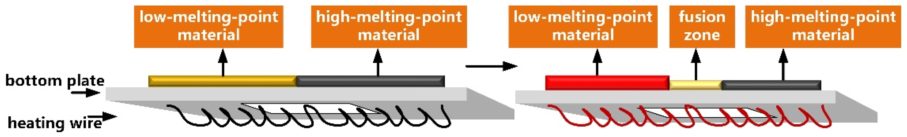
The sparse and dense winding of the heating wire, the design of the insulation unit, and the electronically controlled heating make it easier to attain a controlled temperature gradient. By heating some parts of the sample at high temperatures, the sample is subjected to different temperature gradients, and a semi-molten and semi-solidified state can be achieved. Afterward, the experimental process is observed through the distinctive densities of the same substance in different states and the principles of X-ray transmission imaging [17]. The melting point of pure BiFeO3 is about 960 °C. Co-solvent addition can reduce the melting point up to as low as 800 °C. By utilizing this property, low-melting-point BiFeO3 is placed on the left and the high-melting-point counterpart is placed on the right. Upon heating, the low-melting-point BiFeO3 becomes molten, and the solid-liquid interface appears. The solid-liquid interfaces of the unmelted and molten BiFeO3 can be observed using the X-ray transmission imaging module. The heating process is shown in Figure 4.
After visualizing the data obtained by the X-ray transmission imaging module, the images of the melting and solidification processes of BiFeO3 are obtained as shown in Figure 5. Due to the low contrast of the image obtained by the X-ray transmission imaging module, the solid-liquid interface is unclear, and it is not possible to accurately determine the morphological transformations of BiFeO3 during melting and solidification based on the image. Therefore, it is necessary to propose effective algorithms to process the X-ray images.
3. Image-Enhancement-Related Algorithms
3.1. Histogram Equalization
Histogram equalization is an image processing technique used to adjust the contrast of an image in order to transform the histogram of the original image into a balanced distribution. An image with a non-uniform gray level probability density distribution is turned into a target image with a uniform probability density distribution by seeking a certain gray level transformation. The gray level histogram of an image can be represented as a one-dimensional discrete function, and it describes the frequency or number of each gray level in the image [18]. It can be written as:
where, is the number of pixels with a gray level of in image , denotes the total number of gray levels, and the height of each bin column of the histogram corresponds to . The gray level histogram tells the distributions of all gray levels in the original image. Based on the histogram, the normalized histogram is further defined as the relative frequency of occurrences of gray levels:
where, is the total number of gray levels, denotes the number of pixels of the th gray level, and is the total number of pixels in the original image. Subsequently, the cumulative distribution function of the normalized histogram of the image is calculated:
where, , and it denotes the gray level after normalization, and denotes the gray level before normalization. The original gray level is mapped to the new gray level by the transformation function , while the new gray level is used to replace the corresponding gray level in the original image to obtain an equalized image.
3.2. Wavelet Denoising
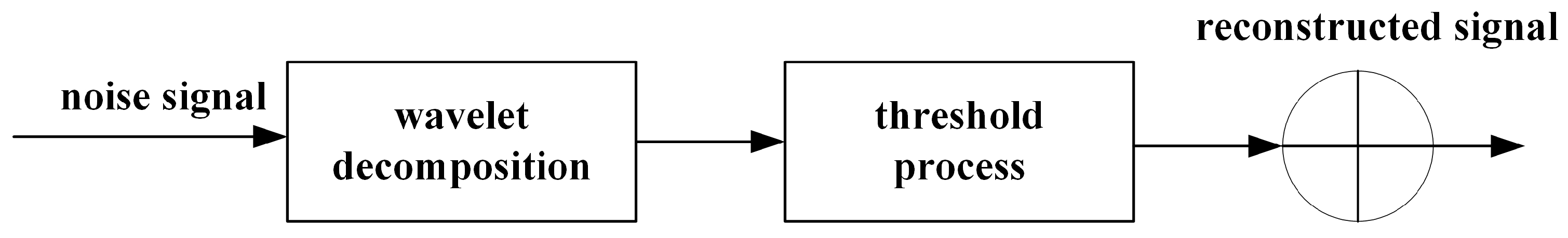
Wavelet denoising performs local denoising of signals or images by combining wavelet transform and thresholding. Wavelet denoising has the advantages of multi-scale adaptiveness, time-frequency localization, and non-stationary signal processing. Wavelet denoising can better preserve the detailed information of the signal or image while removing noise. Its flowchart is shown in Figure 6.
The original signal is represented as a discrete wavelet transform (DWT):
where, denotes the coefficient of the wavelet function at scale , is the coefficient of the wavelet function at scale , denotes the lowest resolution level, and is the total level of wavelet decomposition.
The soft thresholding method is a thresholding technique commonly used in wavelet denoising to reduce the magnitude of the wavelet coefficients and thus reduce noise. It can effectively suppress noise while preserving the details of the signal. This method is based on thresholding the magnitude of the wavelet coefficients. Specifically, smaller wavelet coefficients are set to zero, thus suppressing the effects of noise. In the meantime, larger wavelet coefficients preserve the detailed features of the signal, so that the denoised signal is high-quality and high-definition.
For wavelet coefficient , soft thresholding is expressed as follows:
where, is the wavelet coefficients after soft thresholding, is the sign function of , is the absolute value of , and is the soft threshold. The core of soft thresholding is that if the absolute value of is less than the threshold , then it is set to zero. Otherwise, its original value is retained. The soft thresholding method helps to remove the low-amplitude noise components in the wavelet coefficients while retaining the larger-amplitude components of the signal, thus realizing signal denoising. Choosing the right threshold value usually requires adjustments according to the specific applications and signal characteristics.
4. Gradient Three-Interval Equalization Image Contrast Enhancement Algorithm Combined with Improved Adaptive Contrast Enhancement
In order to enhance the contrast of X-ray images in melting and solidification experiments of high-temperature materials, this paper proposes the GTIE-IACE. This algorithm aims to improve overall image contrast and enhance local detail definition. The flowchart of the GTIE-IACE algorithm is shown in Figure 7.
4.1. Image Preprocessing
First of all, the images are denoised. Images of melting and solidification experiments of high-temperature materials are preprocessed via wavelet denoising with the help of soft thresholding. The threshold is selected based on the average noise intensity to filter out the noise below the threshold. The mean value of an image is calculated and used as an estimate of the noise. The threshold is then selected based on the noise level. The process can be expressed using the following equations:
where, is the number of pixels in the image, is the intensity of the th pixel, and denotes a constant with a value of 2.
4.2. Improved Adaptive Contrast Enhancement(IACE)
Different from traditional global contrast enhancement algorithms, the adaptive contrast enhancement algorithm [19] adjusts the intensity of contrast enhancement based on local features. Combined with the adaptive contrast enhancement algorithm to improve the dynamic range utilization of the image, the local gray level information within each gradient level is corrected. Assuming is a pixel point in the image, the image window size is set to centered on . The local mean and local variance within each gradient level are represented as follows:
where, is the mean value in the window region centered on pixel point , is the variance in the window region centered on pixel point , and is the total number of pixels in the window region centered on pixel point . The mean value can be approximated as the background part, when is the high-frequency part. Multiplying the gain factor for the high-frequency part can enhance the details in the image. In this paper, we modified the calculation method of the gain factor based on adaptive contrast enhancement so that the gain factor is inversely proportional to the local mean-square error. This processing can be represented as follows:
In the high frequency part of the image, the local variance is larger and the value of the gain factor is smaller. However, in the smoothed region, the local mean-square error is smaller, and the gain factor increases, which causes the amplification of the noise, so it is necessary to make some limitations on the maximum value of the gain factor to obtain better results. In this paper, the global mean-square error is used as the value of parameter to avoid the gain factor being too large.
After being processed by the IACE, the contrast of the image is enhanced, resulting in a new gray level mapping.
4.3. Gradient Three-Interval Equalization Algorithm Combined with Improved Adaptive Contrast Enhancement (GTIE-IACE)
After applying the IACE to obtain a new gray level mapping of the image, the image gradient is divided into three intervals. By dividing the gradient into three intervals, the details and contrast of the image in different gradient ranges are better displayed and enhanced.
First, the gradient information of the pixel points in the image is obtained by performing a convolution operation on the image by the Sobel operator. Given that the gradient of the image at is denoted as , and that is the input image, the following is obtained:
After calculating the gradient of each pixel, the Canny edge detection algorithm is used to further emphasize the edges of the image, retain the edge gradients, and set the non-edge regions to zero.
The gradient strengths are categorized into three classes. Smaller gradient strengths indicate smooth regions or insignificant edge structures in the image. Regions with moderate gradient strengths contain some slight edges or texture features in the image. Lastly, regions with higher gradients have noticeable edges, textures, or structures. The gradient strength is divided into three intervals by two thresholds, and :
Edge points often correspond to the boundaries of objects, textures, or structures in an image, while these boundaries are associated with details of interest, so a large number of edge points are usually present when a region contains rich details [20]. In this paper, the ratio of the number of edge point pixels within each gradient interval to the total number of edge point pixels was used as the weighting factor for each gradient interval. This can more accurately reflect the degree of contribution of each gradient interval to the image details. This processing is expressed as:
where, , , and are the weighting factors of the three gradient intervals. Each pixel in the original image is assigned a specific gradient weighting factor based on the gradient strength, and the weighting coefficient is determined according to the percentage of edge points in the corresponding gradient interval. This processing is expressed as:
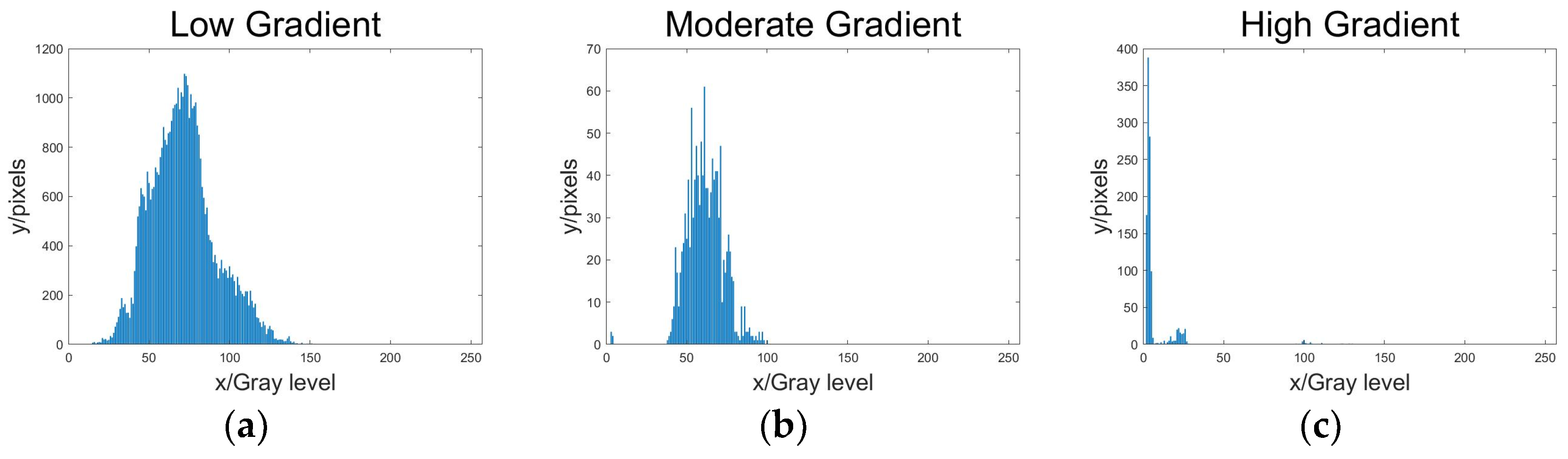
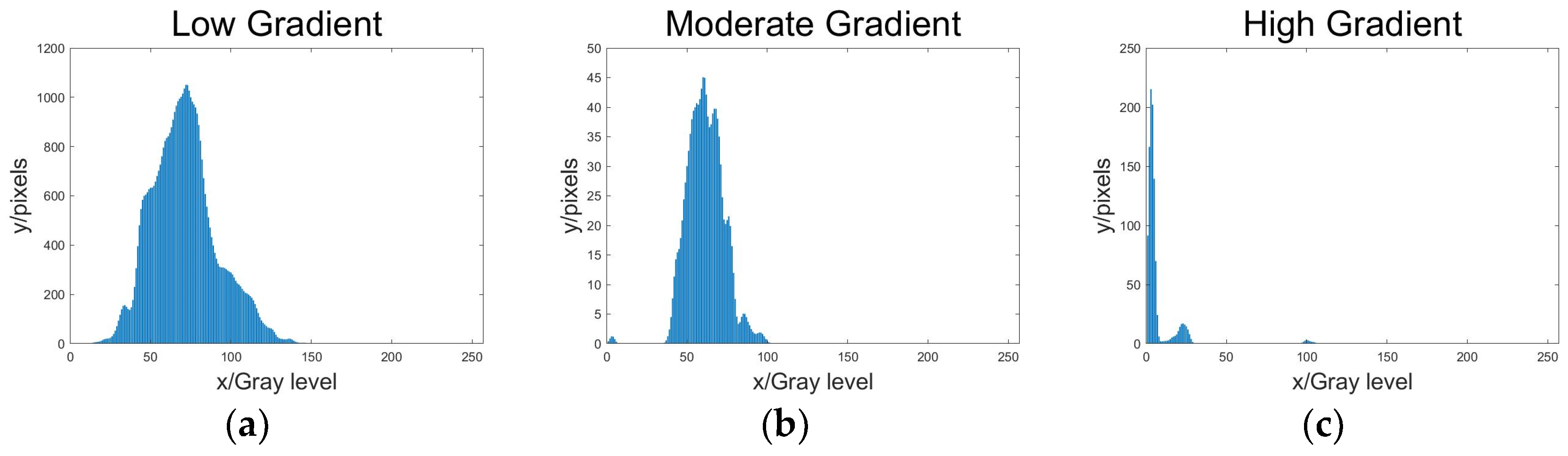
where, is the number of edge points for each gradient level. The number of edge point pixels for each gray level in each gradient interval is shown in Figure 8.
The histogram of edge points in the gradient interval for an X-ray image with unclear texture details is usually in the form of a single narrow peak, as shown in the three panels of Figure 8. If the peak shape becomes flat, the distribution of pixels of different gray levels within the gradient level will be more even and the texture details of the image become sharper. The distribution of the number of pixels at the edge points of each gray level in the gradient interval is processed using a Gaussian function, which is defined as:
where, is a random variable, and and are the parameters of the Gaussian function. is the mean value of and it is used to adjust the positions of the Gaussian peaks, while is the variance of and it determines how flat the peaks are. The larger the value of is, the flatter the peak becomes. In this paper, the values of and are defined as follows:
where, denotes all gray levels, denotes the th gray level. is the probability density of the th gray level, which is the number of edge points within the th gray level divided by the total number of edge points, and is a constant. When becomes larger, the image detail enhancement is more significant. To prevent excessive sharpening of the image, a value of is adopted. According to Figure 9, after using the Gaussian function to process the histograms of edge points in different gradient intervals, the peaks become flatter.
After obtaining the numbers of edge pixel points for all grey levels in different gradient intervals, weighted summation is performed using the relative weights of the gradients and the numbers of edge pixel points. This can be expressed by the below equation:
where, denotes the number of edge points in the th gradient interval, and denotes the relative weight of the edge points in the th gradient interval.
Lastly, the number of edge points at each grey level within different gradient intervals is statistically analyzed to obtain the distribution of edge points at each grey level within each gradient interval. It can be written as:
Assuming the size of the image is and the position of pixels is . denotes the total number of edge points in the th grey level and the th gradient level. denotes the gradient value at pixel point . As shown in Equation (10), denotes the gray level at pixel point . For each pixel point, is used to determine whether the gradient level is equal to , and is used to determine whether the grey level is equal to . When both the gradient value and gray level satisfy the condition, the value of the item is 1; otherwise, it is 0. Due to the use of the Canny edge detection algorithm to set the gradient value of non-edge pixels to zero, by summing up all the pixel points that satisfy the condition, the number of edge points in the th grey level and the th gradient interval can be obtained.
In the GTIE-IACE process, the number of edge points in each gradient interval is used as the relative weight and then multiplied by the number of edge points at each grey level in each gradient interval. This aims to emphasize the edges in each gradient interval in order to better preserve and enhance these features. It can be written as:
where, is a row vector, in which each element represents the ratio of the number of edge points in the corresponding gradient level relative to the total number of edge points, and is a 3 × 256 vector, where each row corresponds to a gradient level and each column corresponds to a grey level. As shown in Equation (22), in the matrix, the element represents the number of edge points in the th gradient interval and the th grey level. can be expressed more intuitively using a histogram (Figure 8). Each element of represents the degree of contribution of the different gradient levels to the image details. This vector serves as a comprehensive representation of the edge point information at all different gradient levels. Based on this, the relative frequency of gradient level occurrences is further defined as follows:
Finally, the cumulative distribution function of the normalized image is computed. The original gradient levels are mapped to the new gradient levels through transformation, and the gradient levels in the original image are replaced by the new ones. The GTIE-IACE algorithm is illustrated in Figure 10.
5. Evaluation Metrics
In the process of melting and solidification experiments of high-temperature materials, there is no reference image available for comparison. Therefore, the solid-liquid interface image contrast enhancement algorithm was evaluated in this paper using the Non-Reference Image Quality Assessment (NR-IQA).
5.1. Contrast Enhancement Based Contrast-Changed Image Quality Measure (CEIQ)
In the existing NR-IQA studies, image contrast is a very important metric [21]. Jia Yan et al. [22] proposed an effective metric to evaluate the performance of contrast enhancement algorithms in the absence of reference images.
The method first generates an enhanced image and calculates the similarity between the original and enhanced images using the structural similarity index (SSIM) as the first feature. Subsequently, the entropy and cross-entropy between the original and enhanced images are calculated separately to obtain the sum of the four features. Finally, a regression module is used to fuse these five features to obtain the evaluation score. The similarity calculation of SSIM is as follows:
where, and are two images, , , and represent the similarity between the two images in terms of brightness, contrast, and structure, and , , and denote the relative importance of the brightness, contrast, and structural similarity in SSIM. CEIQ uses SSIM as its first evaluation feature.
Histograms provide image contrast information, so CEIQ utilizes histograms as the second metric. Entropy is a concept in information theory used to measure the uncertainty or information content of a random variable. It is a metric that quantifies the probability distribution of the random variable. The histograms of both high-contrast and contrast-enhanced images tend to have uniform distributions. In other words, they have high entropy. The entropy of a histogram can be expressed as:
where, b denotes the value of the bin of the histogram. By using cross-entropy, the relationship between the input grey level histogram and the equalized histogram is considered, and it is calculated by the formula below:
For any image, CEIQ utilizes image similarity , histogram-based entropy and , and cross entropy and to give a feature vector . Next, with the help of feature vectors and subjective scores of images , a training set can be constructed, and a regression function can be learned. CEIQ uses the LIBSVM package and linear kernels to implement support vector regression and uses the regression model to evaluate the quality of input images.
5.2. Measure of Enhancement (EME)
Panetta et al. [23] proposed another NR-IQA, a contrast-based enhancement metric to quantify the value of contrast enhancement obtained in an image. The EME can be expressed as:
where, are the number of blocks in the horizontal and vertical directions of the image. are the maximum and minimum gray levels within the image blocks. A higher EME score indicates that the algorithm gives a better contrast enhancement effect.
5.3. Measure of Entropy (MOE)
The entropy of an image can be considered as a statistical parameter characterizing the complexity of the image texture and information density. The entropy of an image can be expressed as:
where, represents the entropy of the image, represents the probability of the th gray level occurring in the image. is utilized to assess the amount of information in the image. A higher entropy value indicates a more uniform distribution of pixel values, resulting in a higher level of texture and detail in the image [24].
6. Experimental Results
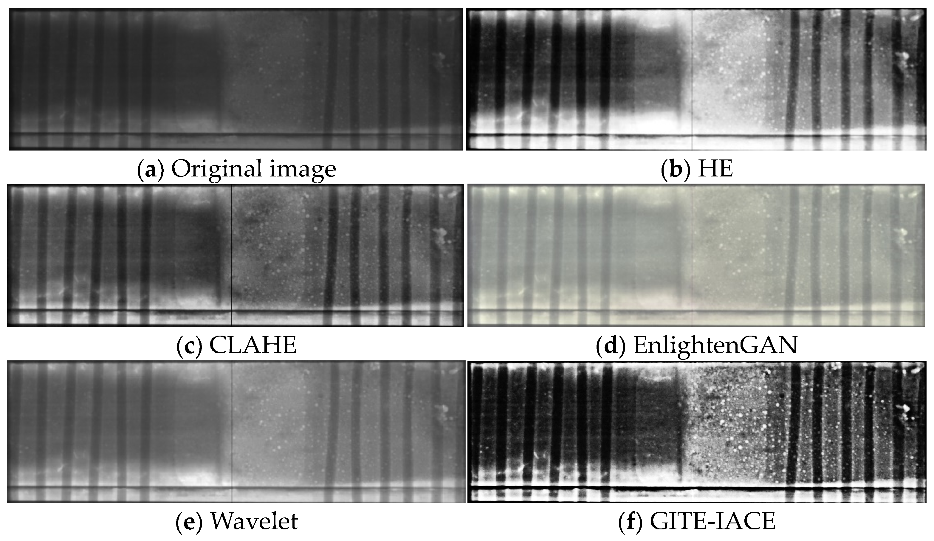
As shown in Figure 11, more detailed information can be observed after image enhancement using the GTIE-IACE algorithm. In contrast, although HE and CLAHE [21] can equalize the histogram of the image, these two algorithms are not effective in processing the microstructural changes during melting and solidification of BiFeO3.
Oscillations and artifacts appear during wavelet decomposition and reconstruction. The wavelet transform is an operation based on local windows. When the window intersects with the image boundary, this results in incomplete data at the boundary, thus introducing oscillations and artifacts.
EnlightenGAN is an efficient unsupervised generative adversarial network that provides satisfactory low-light image enhancement by using deep learning and generative adversarial network techniques [25]. However, EnlightenGAN is not effective in processing images of melting and solidification of high-temperature materials. Although the overall brightness of the image is improved, there is no significant change in the contrast and the detail information is not clear.
The GTIE-IACE algorithm proposed shows a better performance. The algorithm is able to more effectively enhance the details of the melting and solidification processes while improving the brightness and contrast of the image. This means that the GTIE algorithm has an advantage in extracting and enhancing the key details and hence is a better choice for processing this particular type of image.
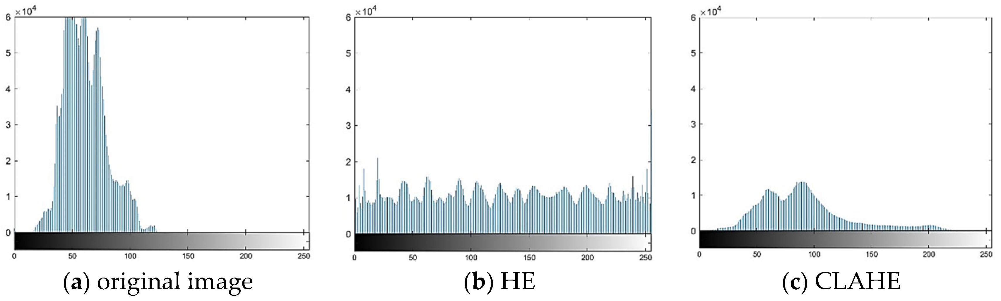
According to the histograms, the grey level values of the image enhanced using the GTIE algorithm effectively cover the entire grey level range. This indicates the best enhancement performance among different algorithms (Figure 12).
A gradient histogram is a statistical graph that describes the distribution of gradients of an image. In image processing, the gradient indicates the magnitude of pixel intensity changes in an image. The shape of the gradient histogram reflects the edge features and texture information of the image, and it helps to understand the structure and content of the image. Analyzing gradient histograms is a common means in image processing and computer vision tasks. The gradient histograms of enhanced high-temperature material images using different contrast enhancement algorithms are shown in Figure 13. The gradient histograms of the image processed using GTIE-IACE have a more uniform distribution, highlighting image details at different gradient levels.
CEIQ, EME, and MOE are used to evaluate the effectiveness of the image processing algorithms in contrast enhancement. A higher score indicates that the algorithm gives a better contrast enhancement effect. The NR-IQA for each image in Figure 11 is shown in Table 1. Evaluation scores of different image enhancement algorithms, according to which, the GTIE-IACE algorithm performs the best in terms of image contrast enhancement.
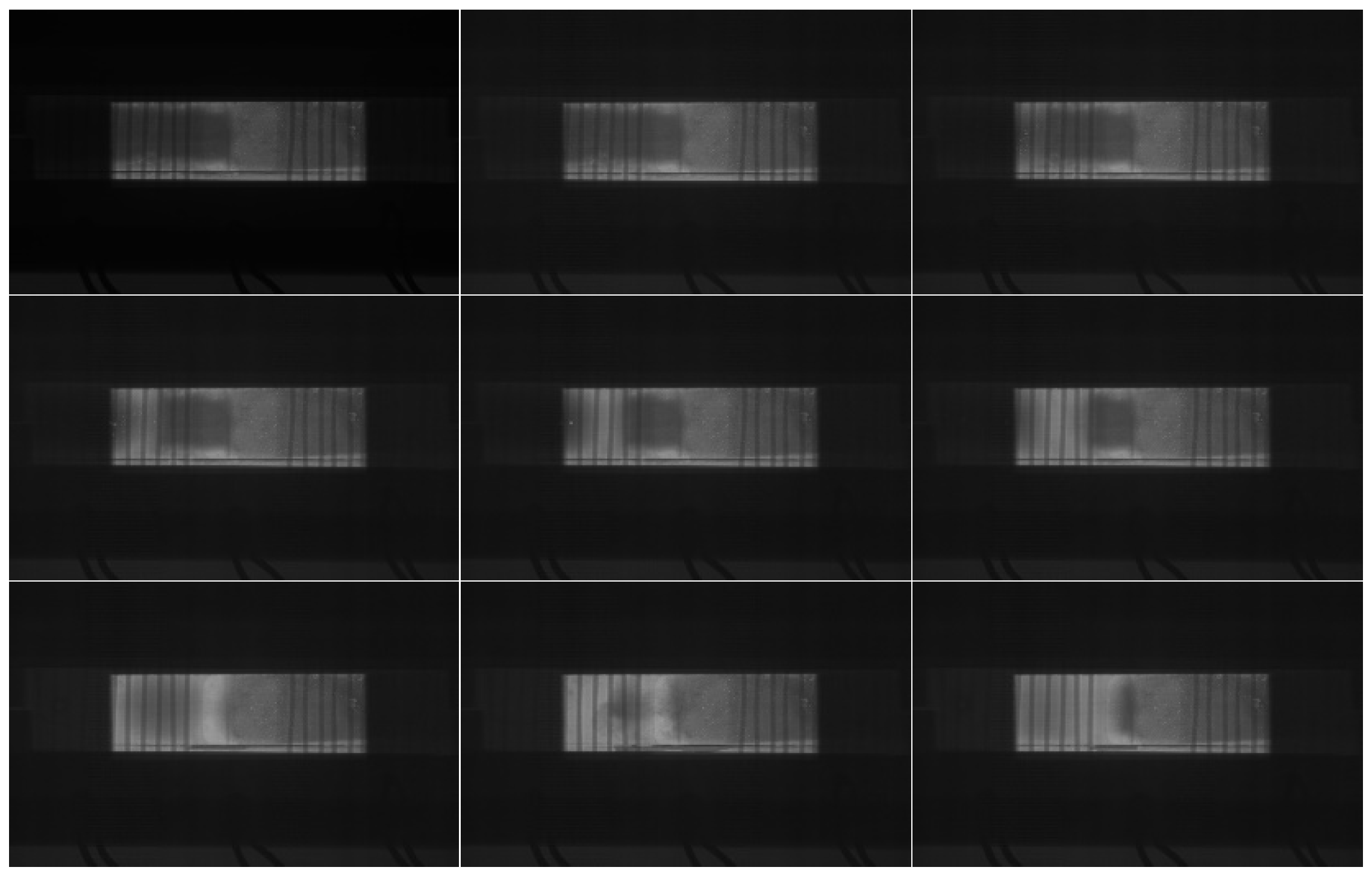
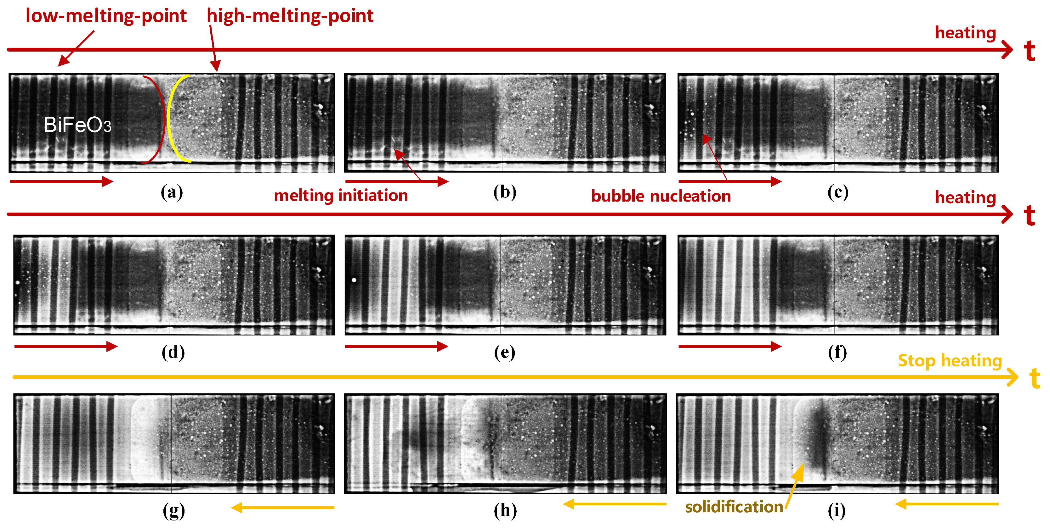
After processing using the proposed solid-liquid interface image contrast enhancement algorithm, the image sequence of the BiFeO3 melting and solidification processes is shown in Figure 14.
Crystal growth kinetics describes the relationship between the velocity of solid-liquid interface movement and the driving force, where the driving force is usually expressed as undercooling, which can be obtained through temperature gradients. In order to accurately study crystal dynamics, a clear solid-liquid interface is a necessary condition. If the solid-liquid interface is not clear, it will affect the accuracy of the kinetic function.
The algorithm proposed in this paper significantly improves the contrast of the solid-liquid interface in the image, thereby obtaining a clearer solid-liquid interface. It can better understand the growth mechanism of crystals and extract more accurate crystal dynamics functions. By gaining a deeper understanding of the crystal growth mechanism, we can develop corresponding plans to change and optimize the growth process, in order to improve the performance of the crystal. The solid-liquid interface contrast enhancement algorithm plays a crucial role in this process, helping us better understand crystal dynamics and providing important support for optimizing growth mechanisms to improve crystal performance.
During the melting and solidification of BiFeO3, the solid-liquid interface marks the boundary between solid crystals and liquid melts. In Figure 14a–i, low-melting-point BiFeO3 is on the left side of the images. The material starts to melt at 800 °C. On this side, BiFeO3 is in the liquid or semi-solid state during the melting process. On the right side is high-melting-point BiFeO3, which does not melt during the experiment. When BiFeO3 on the left side begins to melt, a BiFeO3 solid-liquid interface will be created so that the crystal growth process can be observed.
Changes in the density of the melt cause changes in the X-ray transmission images, usually because heating causes varying densities over different areas of the melt and changes in X-ray absorption. The denser melts appear as darker areas in the images. In Figure 14a, the marked area on the left side of the image is darker and denser, and it shows stronger X-ray absorption. In the meantime, BiFeO3 still maintains a solid structure at this time and has not begun to melt. The color of BiFeO3 in Figure 14b becomes lighter, and the crystals start to melt. The melting phenomenon of BiFeO3 in Figure 14c is more obvious. After heating, some crystals of BiFeO3 have completely melted. The molten BiFeO3 absorbs less X-rays, and it is in a transparent state. Furthermore, it exhibits a tendency to migrate to the right. From Figure 14b–f, it can be observed that, with the increase in temperature, BiFeO3 melts, and bubbles generated during the melting process appear in the red marked area on the left side. After melting, cooling and solidification are carried out, as shown in Figure 14g–i, with the gradual decrease in temperature, gradual solidification of the melt is observed. The melt region gradually shrinks and eventually changes to a solid state. Eventually, a solidified state is noted in Figure 14i. It marks the completion of the phase transition process.
By observing changes in melting density and X-ray transmission images, the melting and solidification characteristics of BiFeO3 during heating and cooling processes can be revealed. These observation results can provide guidance for space material design and process control.
7. Conclusions
A gradient three-interval equalization image enhancement algorithm combined with improved adaptive contrast enhancement was proposed to enhance the contrast and edge details of X-ray images. The algorithm adjusts the intensity of contrast enhancement based on local features and improves the calculation method of the gain factor in the adaptive contrast enhancement algorithm. Lastly, it introduces a weight calculation strategy for the three gradient intervals. The degrees of contribution of different gradient levels to the image details are adopted as the weights, so the image enhancement process is more targeted. X-ray images of BiFeO3 melting and solidification processes were used for testing the proposed algorithm. The experimental results show that, from the images enhanced by the GTIE-IACE, the detail changes during melting and solidification can be more clearly observed. It should be pointed out that the details of image regions with small differences in brightness changes are also well enhanced. Compared with the traditional image contrast enhancement algorithms, the proposed GTIE-IACE effectively avoids issues such as over-enhancement of global contrast and insignificant contrast enhancement of image regions with small gradient changes. From the processed X-ray images of BiFeO3 melting and solidification processes, distinct solid-liquid interfaces, and crystal growth processes can be clearly observed. By enhancing the contrast and edge details of images, researchers can analyze the phase transition behavior of crystalline materials more easily. This is of great significance for carrying out research based on real-time observation of high-temperature material experimental processes on the space station.
Author Contributions
Conceptualization, X.L. and X.P.; methodology. X.L.; validation, Z.Y.; formal analysis, X.L. and X.P.; investigation, X.L. and X.P.; resources, Q.Y.; data curation, Q.Y.; writing—original draft preparation, X.L.; writing—review and editing, X.L., X.P., Q.Y. and Z.Y.; funding acquisition, Q.Y. All authors have read and agreed to the published version of the manuscript.
Funding
This research was funded by the Guangxi Key Research and Development Program No. AB23026105, Guilin major special plan No. 20220103-1, Special funds for local scientific and technological development under the guidance of the central government in 2021 (GuiKeZY21195030) and Chinese Manned space program.
Institutional Review Board Statement
Not applicable.
Informed Consent Statement
Not applicable.
Data Availability Statement
The raw data supporting the conclusions of this article will be made available by the authors on request.
Conflicts of Interest
The authors declare no conflicts of interest.
References
- Zhao, J.; Du, W.; Kang, Q.; Lan, D.; Li, K.; Li, W.; Liu, Y.C.; Luo, X.; Miao, J.; Wang, Q.; et al. Recent Progress of Microgravity Science Research in China. Chin. J. Space Sci. 2022, 42, 772–785. [Google Scholar] [CrossRef]
- Ngomesse, F.; Reinhart, G.; Nguyen-Thi, H.; Soltani, H.; Zimmermann, G.; Browne, D.J.; Sillekens, W. In situ investigation of the Columnar-to-Equiaxed Transition during directional solidification of Al–20 wt.%Cu alloys on Earth and in microgravity. Acta Mater. 2021, 221, 117401. [Google Scholar] [CrossRef]
- Soltani, H.; Reinhart, G.; Benoudia, M.C.; Ngomesse, F.; Zahzouh, M.; Nguyen-Thi, H. Equiaxed grain structure formation during directional solidification of a refined Al-20wt.%Cu alloy: In situ analysis of temperature gradient effects. J. Cryst. Growth 2022, 587, 126645. [Google Scholar] [CrossRef]
- Wang, J.; Wang, K.J.; Wu, J.L.; Hu, J.; Mou, J.F.; Li, L.; Feng, Y.J.; Deng, Z.S. Preparation of eGaIn NDs/TPU Composites for X-ray Radiation Shielding Based on Electrostatic Spinning Technology. Materials 2024, 17, 272. [Google Scholar] [CrossRef] [PubMed]
- Wang, L.; Hoyt, J.J. Layering misalignment and negative temperature dependence of interfacial free energy of B2-liquid interfaces in a glass forming system. Acta Mater. 2021, 219, 117259. [Google Scholar] [CrossRef]
- Jian, Z.; Xu, T.; Xu, J.B.; Zhu, M.; Chang, F. Development of Solid-Liquid Interfacial Energy of Melt-Crystal. Jinshu Xuebao Acta Metall. Sin. 2018, 54, 766–772. [Google Scholar]
- Tang, J.R.; Mat Isa, N.A. Bi-histogram equalization using modified histogram bins. Appl. Soft Comput. 2017, 55, 31–43. [Google Scholar] [CrossRef]
- Deng, W.; Liu, L.; Chen, H.; Bai, X. Infrared image contrast enhancement using adaptive histogram correction framework. Opt. Z. Licht Elektron. J. Light Electronoptic 2022, 271, 170114. [Google Scholar] [CrossRef]
- Alhajlah, M. Underwater Image Enhancement Using Customized CLAHE and Adaptive Color Correction. Comput. Mater. Contin. 2023, 74, 5157–5172. [Google Scholar] [CrossRef]
- Ye, B.W.; Jin, S.; Li, B.; Yan, S.Y.; Zhang, D. Dual Histogram Equalization Algorithm Based on Adaptive Image Correction. Appl. Sci. 2023, 13, 10649. [Google Scholar] [CrossRef]
- Cui, X.; Lu, D.; Ma, D.; Kang, C.; Sun, J. Research Progress of High Temperature Material Science Experimental Equipment for Space Application. Manned Spacefl. 2023, 43, 455–463. [Google Scholar]
- Zhao, J.; Wang, S.; Liu, Q.; He, Z.; Zhang, W.; Li, K.; Zhou, Z.; Luo, X.; Miao, J.; Zheng, H.; et al. Retrospect and Perspective on Microgravity Science in China. Chin. J. Space Sci. 2021, 41, 34. [Google Scholar] [CrossRef]
- Gong, Y.; Yu, Z.; Wang, J. Application of X-ray 3D lmaging in the Field of Battery Materials Research. Chemistry 2020, 83, 64–70. [Google Scholar]
- Liu, X.K.; Yu, Q.; Pan, X.H.; Yu, Z.H.; Lu, X.X. Image contrast enhancement algorithm for X-ray observation of space materials in situ. J. Instrum. 2022, 17, P06010. [Google Scholar] [CrossRef]
- Liu, X.; Pan, X.; Yu, Z.; Ren, J.; Zhuang, Y.; Yu, Q. A solid–liquid interface enhancement algorithm for X-ray in situ observation of space materials. Mater. Des. 2023, 228, 111852. [Google Scholar] [CrossRef]
- Liu, Y.; Wang, Y.; Ma, J.; Li, S.; Pan, H.; Nan, C.-W.; Lin, Y.-H. Controllable electrical, magnetoelectric and optical properties of BiFeO3 via domain engineering. Prog. Mater. Sci. 2022, 127, 100943. [Google Scholar] [CrossRef]
- Chen, K.; Pan, X.; Deng, W.; Ai, F.; Tang, M.; Zhang, M.; Wen, H.; Gai, L. X-ray Fluoroscopy In Situ Real Time Viewing Device. CN210347498U, 17 April 2019. [Google Scholar]
- Kaur, M.; Kaur, J.; Kaur, J. Survey of Contrast Enhancement Techniques based on Histogram Equalization. Int. J. Adv. Comput. Sci. Appl. IJACSA 2011, 2, 137–141. [Google Scholar] [CrossRef]
- Narendra, P.M.; Fitch, R.C. Real-Time Adaptive Contrast Enhancement. IEEE Trans. Pattern Anal. Mach. Intell. 1981, PAMI-3, 655–661. [Google Scholar] [CrossRef]
- Pu, M.; Huang, Y.; Liu, Y.; Guan, Q.; Ling, H. EDTER: Edge Detection with Transformer. In Proceedings of the 2022 IEEE/CVF Conference on Computer Vision and Pattern Recognition (CVPR), New Orleans, LA, USA, 18–24 June 2022. [Google Scholar]
- Zuiderveld, K.J. Contrast Limited Adaptive Histogram Equalization. In Graphics Gems; Academic Press: Cambridge, MA, USA, 1994; pp. 474–485. [Google Scholar]
- Yan, J.; Li, J.; Fu, X. No-reference quality assessment of contrast-distorted images using contrast enhancement. arXiv 2019, arXiv:1904.08879. [Google Scholar]
- Panetta, K.; Grigoryan, A. A New Measure of Image Enhancement. In Proceedings of the InIASTED International Conference on Signal Processing & Communication, Malaga, Spain, 19–22 September 2000. [Google Scholar]
- Tian, F.; Wang, M.; Liu, X. Low-Light Mine Image Enhancement Algorithm Based on Improved Retinex. Appl. Sci. 2024, 14, 2213. [Google Scholar] [CrossRef]
- Jiang, Y.; Gong, X.; Liu, D.; Cheng, Y.; Fang, C.; Shen, X.; Yang, J.; Zhou, P.; Wang, Z. EnlightenGAN: Deep Light Enhancement without Paired Supervision. IEEE Trans. Image Process. 2019, 30, 2340–2349. [Google Scholar] [CrossRef] [PubMed]
Figure 1.
Schematic diagram of HTMSEC (adapted from [11]). HTMSEC mainly includes a high-temperature furnace module, a sample management module, an X-ray transmission imaging module, a control module, and other subsystems (adapted from [12]).

Figure 2.
Schematic diagram of the X-ray transmission imaging module.
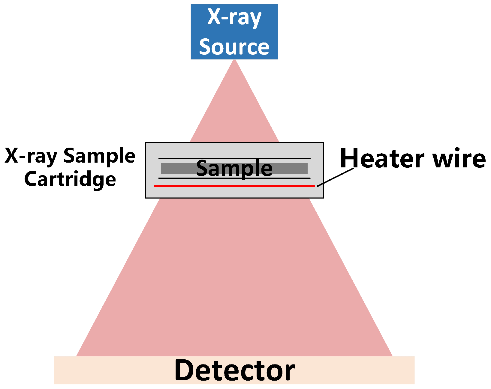
Figure 3.
(a) Schematic diagram of the top cover and the lower plate of the X-ray Sample Cartridge; (b) The high-temperature-resistant ceramic plate.
Figure 3.
(a) Schematic diagram of the top cover and the lower plate of the X-ray Sample Cartridge; (b) The high-temperature-resistant ceramic plate.
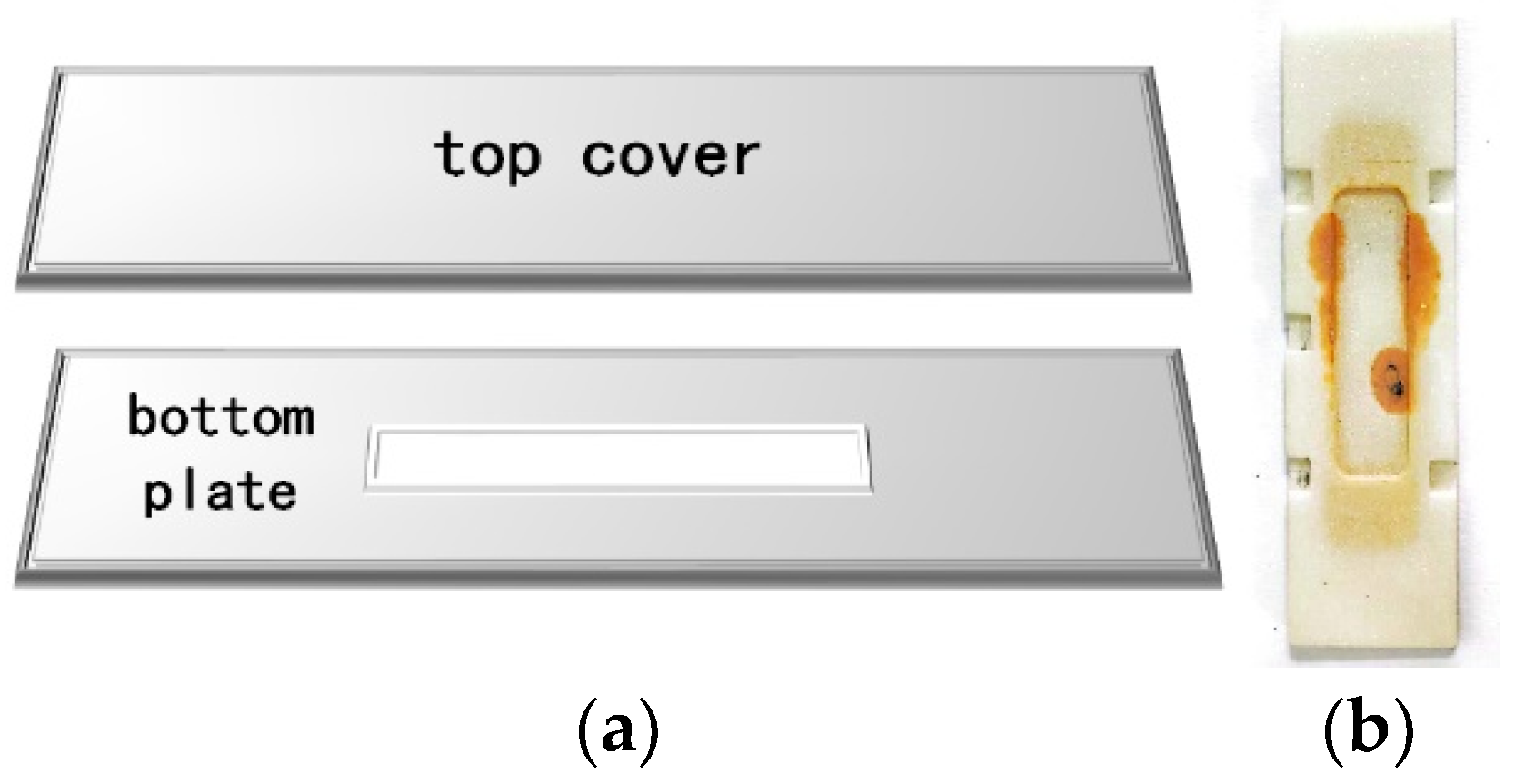
Figure 4.
Schematic diagram of the heating process of high-temperature materials.

Figure 5.
X-ray image sequence of the experimental process of melting and solidification of BiFeO3.

Figure 6.
Schematic diagram of wavelet denoising.

Figure 7.
Flowchart of GTIE-IACE algorithm.
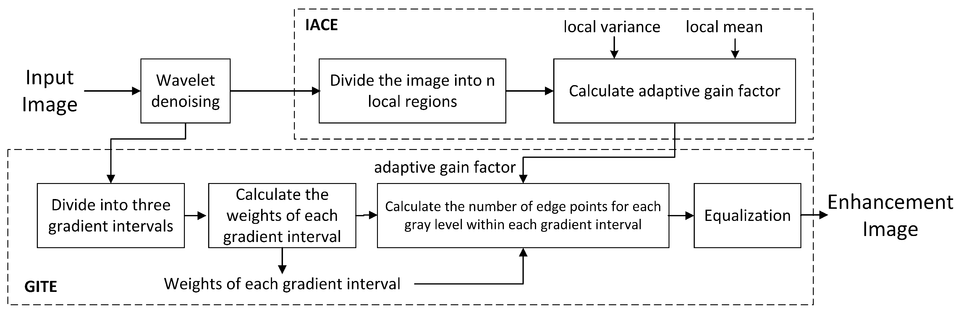
Figure 8.
(a) Histogram of the number of edge point pixels at each gray level in the low gradient interval; (b) Histogram of the number of edge point pixels at each gray level in the moderate gradient interval; (c) Histogram of the number of edge point pixels at each gray level in the high gradient interval.

Figure 9.
(a) Histograms of edge point pixels at each gray level in the low gradient interval after processing; (b) Histograms of edge point pixels at each gray level in the moderate gradient interval after processing; (c) Histograms of edge point pixels at each gray level in the high gradient interval after processing.

Figure 10.
Flowchart of the GTIE-IACE algorithm.
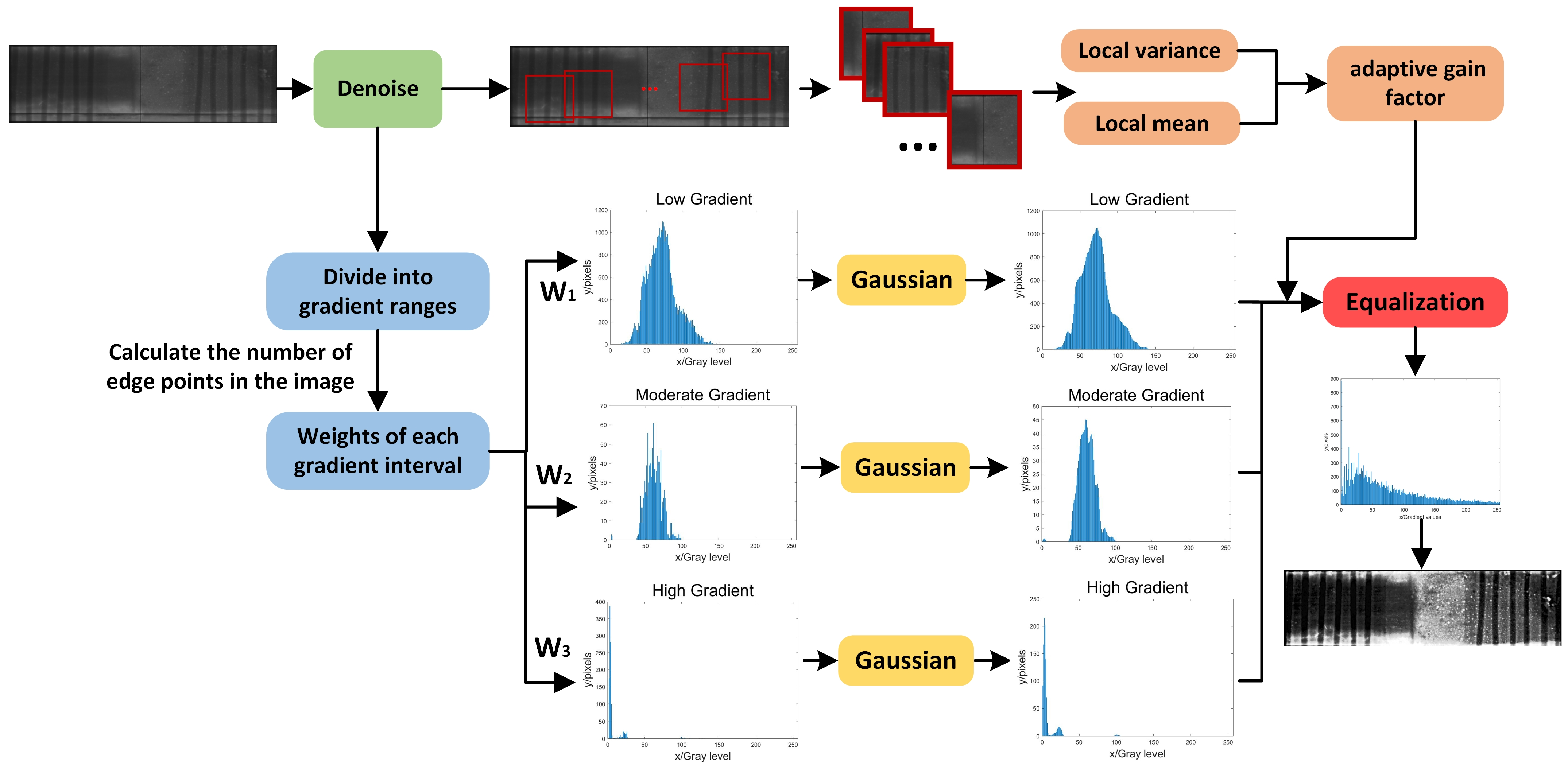
Figure 11.
Processing of BiFeO3 solid-liquid interface images using different contrast enhancement algorithms.
Figure 11.
Processing of BiFeO3 solid-liquid interface images using different contrast enhancement algorithms.

Figure 12.
Gray level histograms of BiFeO3 solid-liquid interface image processed by different contrast enhancement algorithms.
Figure 12.
Gray level histograms of BiFeO3 solid-liquid interface image processed by different contrast enhancement algorithms.


Figure 13.
Gradient histograms of BiFeO3 solid-liquid interface images processed by different contrast enhancement algorithms.
Figure 13.
Gradient histograms of BiFeO3 solid-liquid interface images processed by different contrast enhancement algorithms.
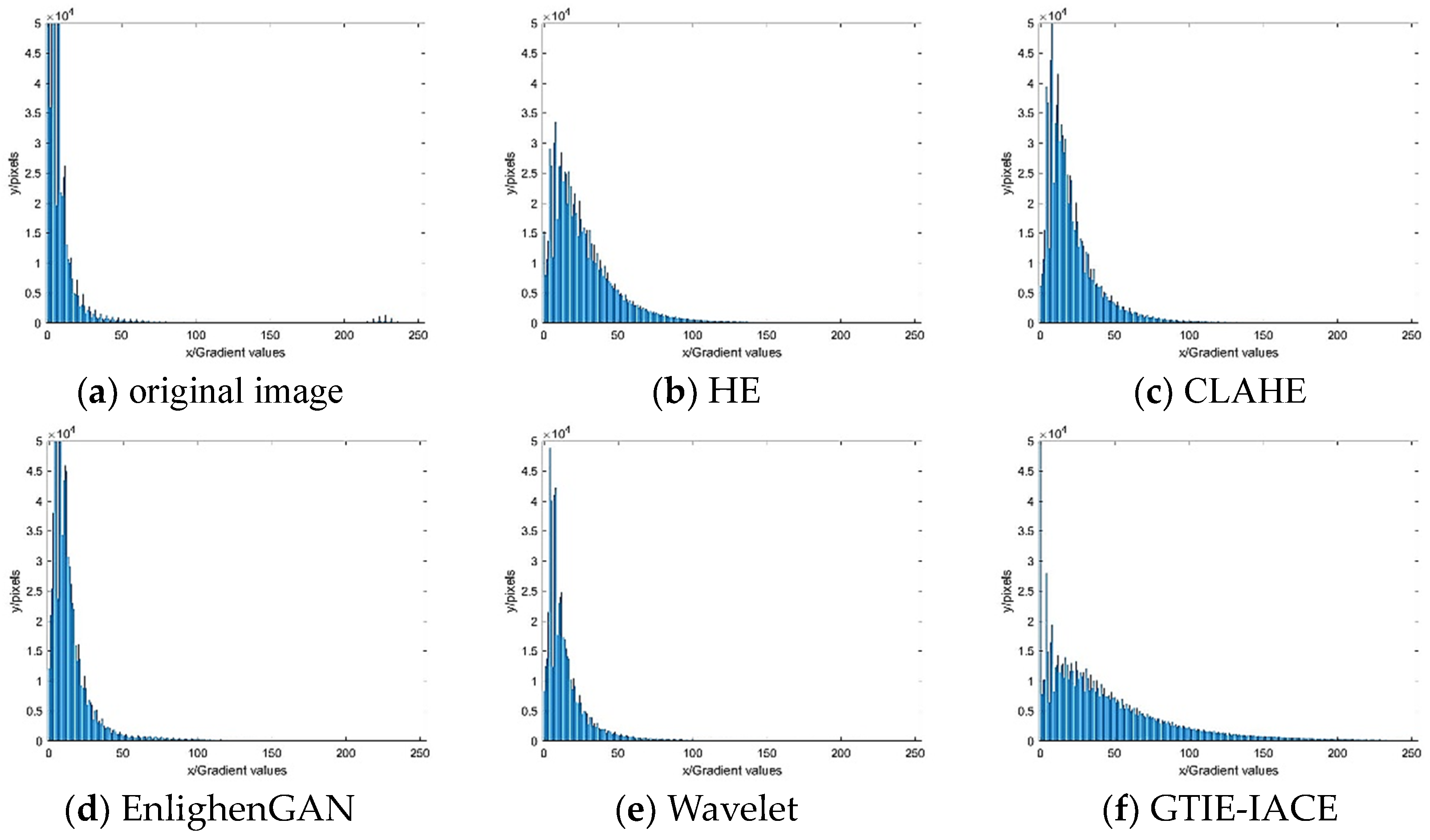
Figure 14.
BiFeO3 solid-liquid interface images processed by GTIE-IACE. (a) shows the beginning of heating BiFeO3; (b–f) shows the heating process of BiFeO3; (g) shows the stop of heating BiFeO3 and the beginning of solidification; (h) shows the solidification process of BiFeO3; (i) shows the complete solidification of BiFeO3 and the end of the experiment.


Table 1.
Evaluation scores of different image enhancement algorithms.
| Method | Evaluation Scores | ||
|---|---|---|---|
| CEIQ | EME | MOE | |
| Original image (a) | 2.289 | 3.765 | 6.065 |
| HE (b) | 4.493 | 12.037 | 7.801 |
| CLAHE (c) | 4.975 | 6.181 | 7.139 |
| EngligntenGAN (d) | 4.201 | 14.2223 | 7.009 |
| Wavelet (e) | 3.303 | 1.8334 | 6.412 |
| GTIE-IACE (f) | 6.512 | 41.0593 | 7.804 |
Disclaimer/Publisher’s Note: The statements, opinions and data contained in all publications are solely those of the individual author(s) and contributor(s) and not of MDPI and/or the editor(s). MDPI and/or the editor(s) disclaim responsibility for any injury to people or property resulting from any ideas, methods, instructions or products referred to in the content. |
© 2024 by the authors. Licensee MDPI, Basel, Switzerland. This article is an open access article distributed under the terms and conditions of the Creative Commons Attribution (CC BY) license (https://creativecommons.org/licenses/by/4.0/).
Share and Cite
MDPI and ACS Style
Li, X.; Yu, Q.; Pan, X.; Yu, Z. Research on the Contrast Enhancement Algorithm for X-ray Images of BiFeO3 Material Experiment. Appl. Sci. 2024, 14, 3546. https://doi.org/10.3390/app14093546
AMA Style
Li X, Yu Q, Pan X, Yu Z. Research on the Contrast Enhancement Algorithm for X-ray Images of BiFeO3 Material Experiment. Applied Sciences. 2024; 14(9):3546. https://doi.org/10.3390/app14093546
Chicago/Turabian StyleLi, Xinze, Qiang Yu, Xiuhong Pan, and Zehua Yu. 2024. "Research on the Contrast Enhancement Algorithm for X-ray Images of BiFeO3 Material Experiment" Applied Sciences 14, no. 9: 3546. https://doi.org/10.3390/app14093546
Note that from the first issue of 2016, this journal uses article numbers instead of page numbers. See further details here.