
Beacon, a Lightweight Deep Reinforcement Learning Benchmark Library for Flow Control

MINES Paristech, CEMEF, PSL—Research University, 1 Rue Claude Daunesse, 06904 Sophia Antipolis, France
*
Author to whom correspondence should be addressed.
Appl. Sci. 2024, 14(9), 3561; https://doi.org/10.3390/app14093561
Submission received: 27 February 2024
/
Revised: 29 March 2024
/
Accepted: 17 April 2024
/
Published: 23 April 2024
(This article belongs to the Special Issue Advances in Active and Passive Techniques for Fluid Flow Manipulation)
Abstract
:Recently, the increasing use of deep reinforcement learning for flow control problems has led to a new area of research focused on the coupling and adaptation of the existing algorithms to the control of numerical fluid dynamics environments. Although still in its infancy, the field has seen multiple successes in a short time span, and its fast development pace is certainly partly imparted by the open-source effort that drives the expansion of the community. Yet this emerging domain is still missing a common ground to (i) ensure the reproducibility of the results and (ii) offer a proper ad hoc benchmarking basis. To this end, we propose beacon, an open-source benchmark library composed of seven lightweight one-dimensional and two-dimensional flow control problems with various characteristics, action and observation space characteristics, and CPU requirements. In this contribution, the seven considered problems are described, and reference control solutions are provided. The sources for the following work are publicly available.
1. Introduction
In recent years, the area of deep-reinforcement-learning-based flow control has undergone a rapid development, with a surge of contributions on topics such as (but not limited to) drag reduction [1], collective swimming [2], and heat transfers [3]. Unlike traditional methods, deep reinforcement learning (DRL) enables the learning of complex control strategies directly from data, thereby alleviating the effects of local minima and the generalizability of the algorithm for other scenarios [4]. Yet the inherent reproducibility issues of DRL algorithms [5], as well as the variety of computational fluid dynamics (CFD) solvers and the possible variability of environment design among the different actors of the community, make it hard to accurately compare algorithm performances, thus hindering the general progress of the field. Moreover, the standard DRL benchmarks (such as the mujoco package [6], or the Atari games from arcade learning environments (ale) [7]) have a limited relevance in the context of benchmarking DRL methods for flow control as their dynamics, observation spaces, computational requirements, and action constraints display substantial differences to those of numerical flow control environments.
From a general point of view, flow control problems are characterized by a simulated physics environment spanning over at least two dimensions, possibly including time. The control is performed by an agent that modifies boundary conditions, source terms, or other components of the domain in order to optimize a given objective. A notable difficulty is, therefore, designing a robust and at the same time efficient environment that is able to cope with a wide range of actions while preserving low and stable runtimes [8]. One way of minimizing the computational cost is lumping the Navier–Stokes equations, the backbone of most fluid mechanics problems, by limiting the dimensionality and restricting its terms to the dominant ones for the problem at hand. This way, it is possible to retain the main features of the flow while tuning the schemes and discretizations towards higher performances.
In the present contribution, we lay the first stone of a numerical flow control benchmark library which will allow DRL algorithms to systematically assess methodological improvements on physically and numerically relevant problems. The design of the test cases voluntarily limits the computational cost of the solvers, making this library a first benchmarking step before testing on more complex and CPU-intensive cases.
The organization is as follows: a short presentation of the library and its general characteristics is proposed in Section 2, after which the environments are introduced in a systematic way in Section 3. For each case, the physics of the problem are described, followed by insights on the discretization. Then, the environment parameters and specificities are described, after which baseline learning curves and details on the solved environment are provided. Finally, the perspectives for the present work are exposed in a conclusive section.
2. The beacon Library
This library provides self-contained cases for deep-reinforcement-learning-based flow control. The goal is to provide the community with benchmarks that fall within the range of flow control problems while following three constraints: (i) be written in Python to ensure a simple coupling with most DRL implementations, (ii) follow the general gym application programming interface [8], and (iii) be cheap enough in terms of CPU usage so that training can be performed on a decent computing station. Aligned with the standardized approach of gym, which streamlines environment setup and facilitates a focused exploration of RL research, this library serves as a first step for prototyping flow control algorithms before moving on to larger problems that will require more efficient CFD solvers and, most probably, a CPU cluster.
The original version of the library contains seven cases, whose main characteristics are presented in Table 1. The selection of the cases was made in order to (i) follow the aforementioned constraints and (ii) propose a variety of problem (episodic or continuous) and control (discrete or continuous) types, as well as different action space dimensionalities. For each case, some parameters can be tuned that can significantly modify the difficulty and the CPU requirements of the problem. In their default configurations, two cases have low CPU requirements and can be run on a standard laptop; three have intermediate computational loads and will require an extended running time on a laptop or a workstation and can benefit from the use of parallel environments; and, finally, two have high computational needs and will require a decent workstation and parallel sample collection [9,10]. Some cases, such as rayleigh-v0, lorenz-v0 [3], vortex-v0 [11], and shkadov-v0 [12], were taken from the literature and fully re-implemented, while others were designed specifically for this work. All the environments of the library follow a similar development pattern, and are self-contained to simplify re-usability. If the Python language is not optimal in terms of performance, the core routines are deferred to numba [13] to reduce the execution time. To avoid version conflicts and improve compatibility, additional package requirements are strictly reduced to gym [8], numpy [14], and matplotlib [15].
All environments are solved with an in-house implementation of the proximal policy optimization (ppo) algorithm [16], for which the default parameters are provided in Table 2. Depending on the control type, results obtained from an off-policy algorithm (either deep Q-networks (dqn) [17] or the time-delayed deep deterministic policy gradient (td3) [18]) are also shown for comparison. The performances of these algorithms are evaluated on standard benchmarks in Appendix A.
3. Environments
3.1. Shkadov
3.1.1. Physics
The initial investigation into vertically falling fluid films was conducted by Kapitza and Kapitza [19], sparking extensive experimental exploration in subsequent decades. These experiments revealed that waves on the surface of a descending thin liquid film exhibit strong non-linearity, manifesting the emergence of saturated waves from small perturbations in amplitude, as well as the presence of solitary waves. For low Reynolds numbers (), it was noted that the wavelength of the non-linear waves greatly exceeded the thickness of the film, allowing for potential simplifications in their physical modeling (referred to as the long-wave regime). Various physical models were proposed, among them the Shkadov model, which was introduced in 1967 [20]. Despite being shown to be inconsistent [21], the model exhibits intriguing spatio-temporal dynamics while remaining computationally affordable. The flow rate q and the fluid height h are simultaneously evolved using the following set of equations:
where the parameter encompasses all the physics of the problem,
and where and W are the Reynolds and the Webber numbers, respectively, defined by the flat film thickness and the flat film average velocity [22]. System (1) is solved on a 1D domain of length L with the following initial and boundary conditions:
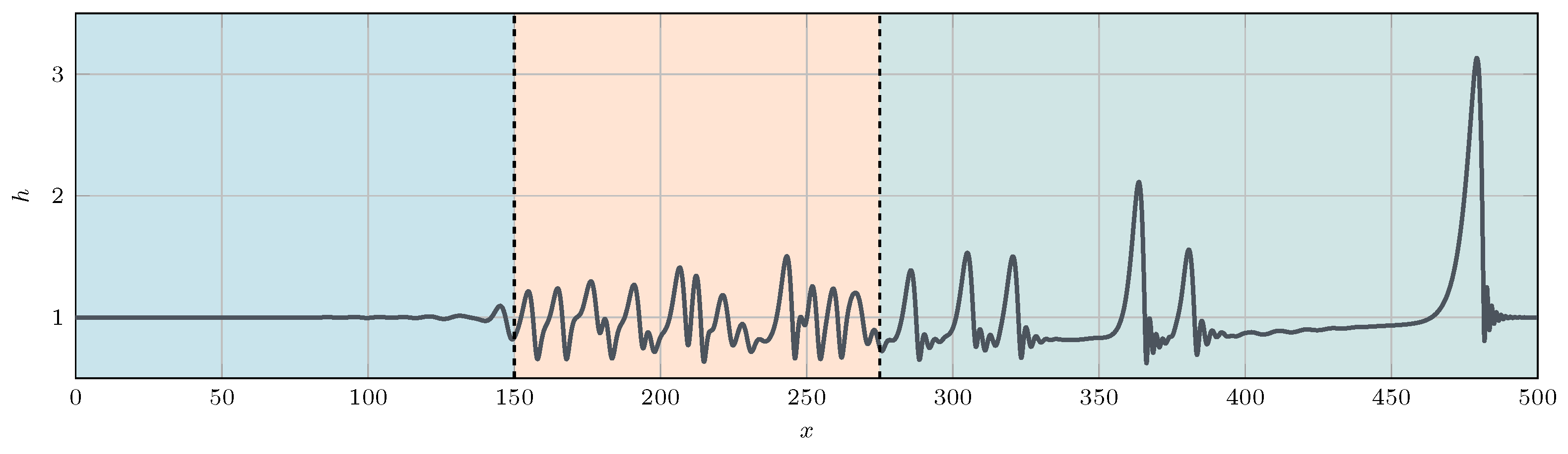
with being the noise level generated by the uniform distribution . As depicted in Figure 1, the introduction of random uniform noise at the inlet initiates the onset of exponentially growing instabilities (blue region), which subsequently exhibit a pseudo-periodic pattern (orange region). In the subsequent area, the periodicity of the waves breaks, and the instabilities transform into pulse-like formations, characterized by a sharp leading edge followed by minor ripples [23]. Of the sharp pulses, some, known as solitary pulses, move faster than others, leading to the amalgamation of upstream pulses in coalescence events. The parameter completely governs the dynamics of these solitary pulses, while the position of the transition region may also be linked to the level of noise at the inlet [22]. It is worth noting that the Shkadov equations have a close relationship with the Kuramoto–Sivashinsky system, which was independently discovered later by Kuramoto and Sivashinsky [24].
3.1.2. Discretization
Equation (1) undergoes discretization employing a finite-difference methodology. Given the presence of abrupt gradients, the convective terms are discretized using a Total Variation Diminishing (TVD) scheme incorporating a minmod flux limiter. The third-order derivative approximation is achieved by combining a second-order centered difference for the second derivative with a second-order forward difference, resulting in the following second-order approximation:
A second-order Adams–Bashforth method is used to integrate the system in time as follows:
where represents the right-hand side of the evolution equation of h in system (1) and is similar for the q field.
3.1.3. Environment
The provided setup is a re-implementation based on the original work by Belus et al. [12], albeit with several distinctions. Notably, the translational invariance aspect introduced in [12] is not utilized in this context. Instead, this control scenario is viewed as an opportunity to evaluate algorithms dealing with problems featuring arbitrarily high action dimensionality.
For the control of system (1), a forcing term is introduced into the equation governing the temporal evolution of the flow rate. Practically, localized jets are inserted at specific locations within the domain, as illustrated in Figure 3 below. The intensities of these jets are determined by the DRL agent. Initially, the first jet is positioned at , with the default jet spacing set to , akin to in [12]. To conserve computational resources, the domain length is conditioned by the number of jets, , and their spacing as follows:
By default, is set to be equal to 150 (which corresponds to the beginning of the pseudo-periodic region for ), and is initialized as 1. The spatial discretization step is designated as , while the numerical time-step is time units. The inlet noise level is configured as , mirroring the setup in [12]. The injected flow rate takes the following form:
where , an ad hoc non-dimensional amplitude factor, and represent the left and right limits of jet j, and denotes the agent-provided jet amplitude. Equation (7) corresponds to a parabolic profile of the jet in x, ensuring a zero flow rate at the boundaries. The jet width is fixed at 4, in line with [12]. To transition from one action to another, a time dependence is introduced to , involving the following saturated linear variation:
Hence, when the actor provides a new action to the environment at time , the effective jet amplitude is linearly interpolated from the previous action to the next one over period (set here to time units). Following this interpolation, the new jet amplitude remains constant for the remainder of time interval (set here to time units). Consequently, the total action time-step is time units. The overall episode duration is fixed at 20 time units, corresponding to 400 actions.
The observations provided to the agent consist of the mass flow rates gathered from the combination of regions of length , located upstream of each jet. In contrast to the original work, the fluid heights in this area are not relayed to the agent, and the observations remain unclipped.
The reward for each jet j is calculated over region of length , positioned downstream of it, with the overall reward being the following weighted summation of individual rewards:
Thus, a perfect flat film yields a maximum reward value of 0. Moreover, the use of a normalization factor enables comparison of scores across different numbers of jets.
Lastly, an evolved initial state is initialized at the onset of each episode. This initial state is derived by solving the uncontrolled equations from an initial flat film setup over a period of time units. For ease of access, this field is stored in a file and loaded at the commencement of each episode. Optionally, the initial state can be randomized by allowing the loaded initial configuration to evolve freely between 0 and 20 time units.
3.1.4. Results
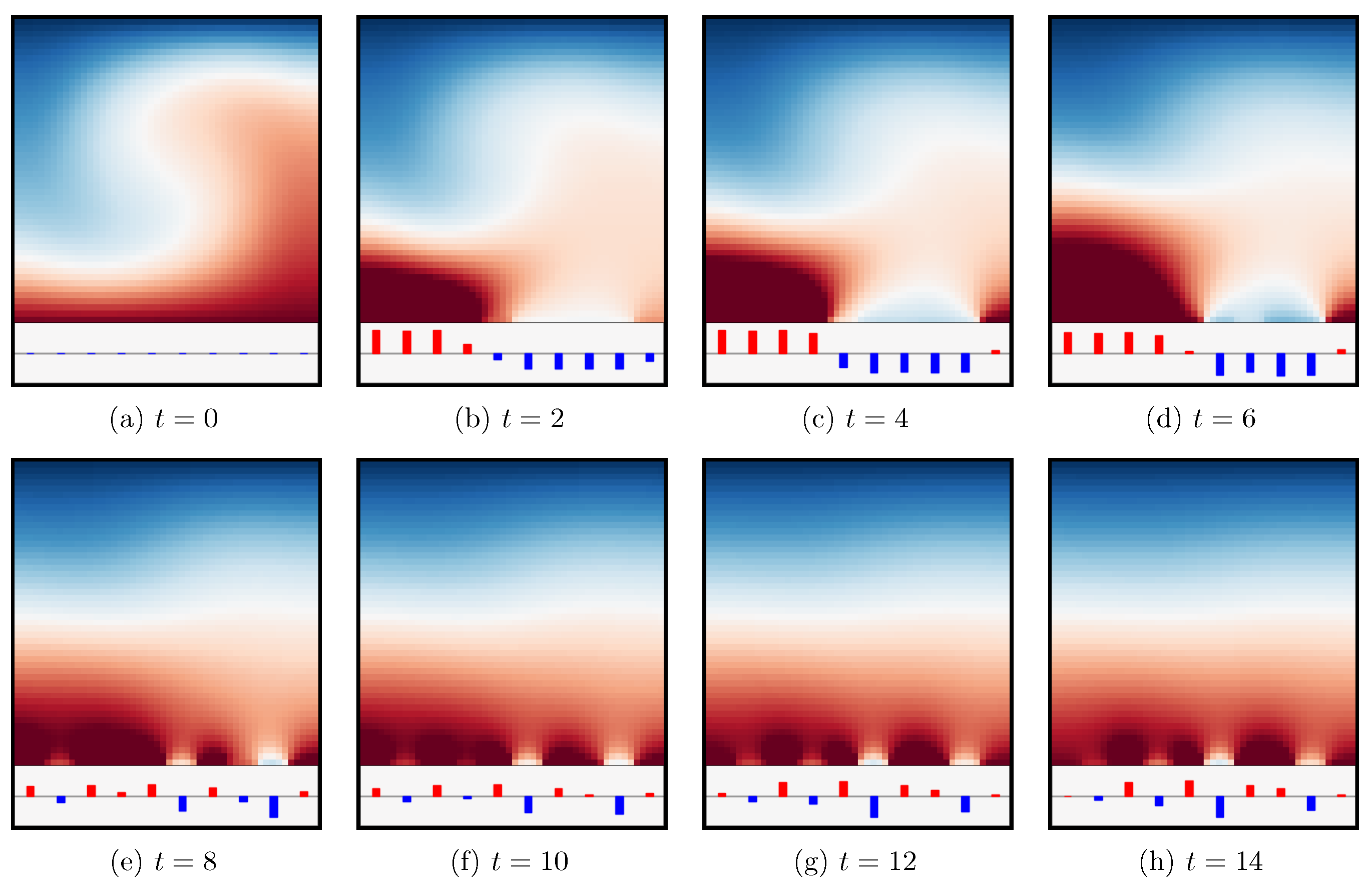
The previously described environment is referred to as shkadov-v0, and its default parameters are provided in Table 3. For the training, we set , , , and k. The related score curves are presented in Figure 2a. We also consider the training on the environment using 1, 5, and 10 jets (see Figure 2b). As could be expected, training is faster for small number of jets, while, for larger numbers of jets, the ppo algorithm struggles due to the increasing dimensionality. In Figure 3, we present the evolution of the field in time under the control of the agent for five jets using the default parameters. As can be observed, the agent quickly constrains the height of the fluid to around before entering a quasi-stationary state in which a set of minimal jet actuations keeps the flow from developing instabilities in their direct vicinity. In the absence of a jet further downstream, the instability regains amplitude at the outlet of the domain. It must be noted that, due to the random upstream boundary condition, the environment is not deterministic, and, therefore, two exploitation runs with the same trained agent would lead to slightly different final scores.
3.2. Rayleigh
3.2.1. Physics
We consider the resolution of the 2D Navier–Stokes equations coupled to the heat equation in a cavity of length L and height H with a hot bottom plate and cold top plate. Under favorable circumstances, this setup is known to lead to the Rayleigh–Bénard convection cell, illustrated in Figure 4. The resulting system is driven by the following set of equations:
where , p, and are, respectively, the non-dimensional velocity, pressure, and temperature of the fluid. The adimensional temperature is described in terms of the hot and cold reference temperatures, respectively denoted as and , as follows:
The dynamics of system (10) are controlled by two adimensional numbers. First, the Prandtl number Pr, which represents the ratio of the momentum diffusivity over the thermal diffusivity as follows:
where is the kinematic viscosity and the thermal diffusivity. Second, the Rayleigh number Ra, which compares the characteristic time scales for transport due to diffusion and convection as follows:
where g is the magnitude of the acceleration of the gravity, and is the thermal expansion coefficient. We also define the instantaneous Nusselt number, Nu, as the adimensionalized heat flux averaged over the hot wall as follows:
System (10) is completed by the following initial and boundary conditions:
In essence, the boundary conditions (12) correspond to (i) a no-slip boundary conditions for the fluid on all boundaries, (ii) imposed hot and cold temperatures on the bottom and top plate, respectively, and (iii) adiabatic boundary conditions on the lateral sides of the domain.
Above critical value , natural convection is triggered in the cell, increasing the heat exchange between the bottom and top regions of the cell, thus leading to a . Illustrations of the temperature and velocity fields are proposed in Figure 4.
3.2.2. Discretization
System (10) is discretized using a structured finite-volume incremental projection scheme with centered fluxes, in the fashion of [25]. For simplicity, the scheme is solved in a fully explicit way, except for the resolution of the Poisson equation for pressure. As is standard, a staggered grid is used for the finite-volume scheme; the horizontal velocity is located on the west face of the cells, and the vertical velocity is on the south face of the cells, while the pressure and temperature are located at the center of the cells. The computation of the instantaneous Nusselt number (11) is performed by computing the first-order finite difference in temperature between the center of the first cell at the bottom of the mesh and the reference temperature . Doing so, we obtain for once the permanent regime is reached, which is close to the reference values found in the literature [26].
3.2.3. Environment
The proposed environment is re-implemented based on the original work of Beintema et al. [3]. In the following, we set , which corresponds to the parameter for air, and in order to avoid excessive computational loads. Similarly to [3], the control is performed by letting the DRL agent adjust the temperature of individual segments at the bottom of the cavity (see Figure 5). To do so, the actions proposed by the agent are continuous temperature fluctuations in the range , with , , and . To enforce and , the provided are normalized as follows [3]:
For simplicity, neither spatial nor temporal interpolations are performed between actions. The spatial discretization step is set as , while the numerical time-step is . The action time-step is equal to 2 time units, with the total episode length being fixed to 200 time units, corresponding to 100 actions.
The observations provided to the agent are the temperatures and the velocity components collected on a grid of probes evenly spaced in the computational domain (see Figure 5) plus the three previous observation vectors. The resulting set of observations is flattened in a vector of size with a default value of .
The reward at each time-step is simply set as the negative instantaneous Nusselt number, such that increasing the reward corresponds to a decrease in the temperature convection as follows:
Finally, each episode starts with the loading of a fully developed initial state obtained by solving the uncontrolled equations during a time of time units. The initial state corresponds to the field shown in Figure 4. For convenience, this field is stored in a file and is loaded at the beginning of each episode.
3.2.4. Results
The environment described in the previous section is referred to as rayleigh-v0, and its default parameters are provided in Table 4. In this section, we note that the entropy bonus for the ppo agent is reduced to compared to the default hyperparameters of Table 2. For the training, we set , , , and k The score curves obtained are presented in Figure 6, while the time evolution of the Nusselt number for the controlled versus uncontrolled cases is shown in Figure 7. As can be observed, the agent manages to devise a set of transition actions toward a stationary state with . The results of Figure 7 are in line with those of [3]. In Figure 8, we present the evolution of the temperature field during the first steps of the environment under the control of the agent using the default parameters.
3.3. Mixing
3.3.1. Physics
We consider the resolution of the 2D Navier–Stokes equations coupled to a passive scalar convection–diffusion equation in a cavity of length L and height H with moving boundary conditions on all sides. The resulting system is driven by the following set of equations:
where and p are, respectively, the non-dimensional velocity and pressure of the fluid, and c is the concentration of a passive species. The dynamics of system (15) are controlled by two adimensional numbers. First, the Reynolds number Re, which represents the ratio between inertial and viscous forces as follows:
where U and L are, respectively, the reference velocity and length values, and is the kinematic viscosity of the fluid. Second, the Péclet number Pe, which represents the ratio between the advective and diffusive transport rates as follows:
where D is the diffusion coefficient of the considered species. In essence, a system with a high Pe value presents a negligible diffusion, and scalar quantities move primarily due to fluid convection. System (15) is completed by the following initial and boundary conditions:
where is the indicator function, and , , , and are user-defined values. In essence, the boundary conditions (16) correspond to a multiple-lid-driven cavity, where tangential velocity can be imposed independently on all sides with an initial patch of concentration in the center of the domain. Snapshots of the evolution of the system in time with are presented in Figure 9.
3.3.2. Discretization
System (15) is discretized using a structured finite-volume incremental projection scheme with centered fluxes. For simplicity, the scheme is solved in a fully explicit way, except for the resolution of the Poisson equation for pressure. As is standard, a staggered grid is used for the finite-volume scheme; the horizontal velocity is located on the west face of the cells, and the vertical velocity is on the south face of the cells, while the pressure and concentration are located at the center of the cells.
3.3.3. Environment
In the following, we set , , , , and . The control is performed by letting the agent adjust the tangential velocities at the boundaries of the domain. We use a discrete action space of dimension 4 with the following actions:
where . The non-dimensional numbers are chosen as and , corresponding to a low-diffusion species. For simplicity, no temporal interpolation is performed between actions. The spatial discretization step is set as , while the numerical time step is . The action time-step is equal to time units, with the total episode length being fixed to 50 time units, corresponding to 100 actions. The observations provided to the agent are the concentration and the velocity components collected on a grid of probes evenly spaced in the computational domain plus the three previous observation vectors. The resulting set of observations is flattened in a vector of size with a default value of . The reward at each time-step is simply set as the average absolute distance of the concentration field to a target uniform value as follows:
Finally, each episode starts with a null velocity field and an initial square patch of concentration , as shown in Figure 9a.
3.3.4. Results
The environment described in the previous section is referred to as mixing-v0, and its default parameters are provided in Table 5. For the training, we set , , , and k. The score curves are presented in Figure 10, along with the score obtained with constant control , which leads to a score of approximately . For comparison, the score with no mixing at all (i.e., pure diffusion) yields a score of . In Figure 11, we present the evolution of the concentration field of the environment under the control of the agent using the default parameters.
3.4. Lorenz
3.4.1. Physics
We consider the Lorenz attractor equations, a simple non-linear dynamical system representative of thermal convection in a two-dimensional cell [27]. The set of governing ordinary differential equations reads:
where is related to the Prandtl number, is a ratio of Rayleigh numbers, and is a geometric factor. Depending on the values of the triplet , the solutions to Equation (20) may exhibit chaotic behavior, meaning that arbitrarily close initial conditions can lead to significantly different trajectories [28], of which one common triplet is , which leads to the well-known butterfly shape presented in Figure 12. The system has three possible equilibrium points, one in and one at the center of each “wing” of the butterfly shape, the characteristics of which depend on the values of , , and .
3.4.2. Discretization
3.4.3. Environment
The proposed environment is re-implemented based on the original work of Beintema et al. [3], where the goal was to maintain the system in the quadrant. Control (20) is performed by adding an external forcing term to the equation as follows:
where u is a discrete action in . The action time-step is set to time units, and, for simplicity, no interpolation is performed between successive actions. A full episode lasts 25 time units, corresponding to 500 actions. The observations are the variables and their time derivatives , while the reward is set to for each step with or 0 otherwise. Each episode is started using the same initial condition .
3.4.4. Results
The environment described in the previous section is referred to as lorenz-v0, and its default parameters are provided in Table 6. In this section, we note that the entropy bonus for the ppo agent is reduced to compared to the default hyperparameters of Table 2. For the training, we set , , , and k. The related score curves are presented in Figure 13. As can be observed, although the learning is successful, it is particularly noisy compared to some other environments presented in this library. This can be attributed to the chaotic behavior of the attractor, which makes the credit assignment difficult for the agent. A plot of the time evolutions of the controlled versus uncontrolled x parameter is shown in Figure 14. As can be observed, the agent successfully locks the system in the quadrant, with the typical control peak also observed by Beintema et al. noted with a red dot in Figure 14. For a better visualization, several 3D snapshots of the controlled system are proposed in Figure 15.
3.5. Burgers
3.5.1. Physics
The inviscid Burgers equation was first introduced by Bateman in 1915 and models the behavior of a one-dimensional inviscid incompressible fluid flow [30] and was then studied by Burgers in 1948 [31].
We consider the resolution of the Burgers equation on a domain of length L along with the following initial and boundary conditions:
where is the noise level introduced at the inlet, and is a constant value. The convection of the random inlet signal leads to a noisy solution in the domain, as is depicted in Figure 16. The initial perturbations steepen while propagating downstream to eventually form shocks.
3.5.2. Discretization
The Burgers equation, Equation (21), is discretized in time with a finite-volume approach. The convective term is discretized using a TVD scheme with a Van Leer flux limiter, while the time marching is performed using a second-order finite-difference scheme.
3.5.3. Environment
The goal of the environment is to control pointwise forcing source term on the right-hand side of (21) in order to damp the noise transported from the inlet. The forcing is applied at , while the length of the domain is set to . The actions provided to the environment, which are expected to be in , are then scaled by an ad hoc non-dimensional amplitude factor . The field is initially set to be equal to , and the variance of the inlet noise is chosen to be . The spatial discretization step is set to , while the numerical time-step is equal to time units. The action duration is set to time units for a total episode duration equal to 10 time units, corresponding to 200 actions. The observations provided to the agent are the values of u upstream of the actuator. Finally, the reward is computed as:
3.5.4. Results
The environment described in the previous section is referred to as burgers-v0, and its default parameters are provided in Table 7. For the training, we set , , , and k. The score curves obtained are shown in Figure 17, while snapshots of the evolution of the controlled environment are shown in Figure 18. As can be observed, the agent successfully damps the transported inlet noise following an opposition control strategy.
3.6. Sloshing
3.6.1. Physics
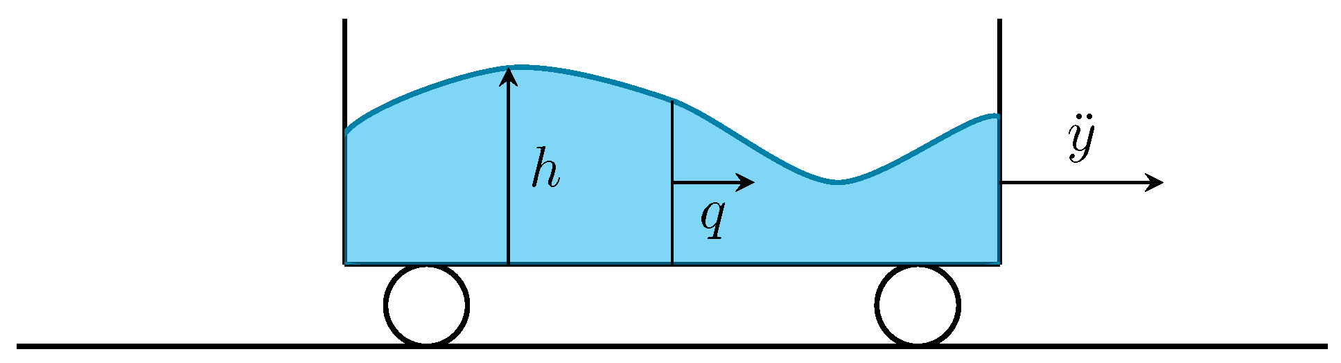
We consider the resolution of the 1D Saint–Venant equations (or shallow-water equations), established in 1871 [32], which describe a shallow layer of fluid in hydrostatic balance with constant density. This system is considered in the context of a mobile water tank of length L subjected to an acceleration , leading to the following equations in the tank referential [33]:
where h is the fluid height, and q is the fluid flow rate. System (24) is completed by the following initial and boundary conditions:
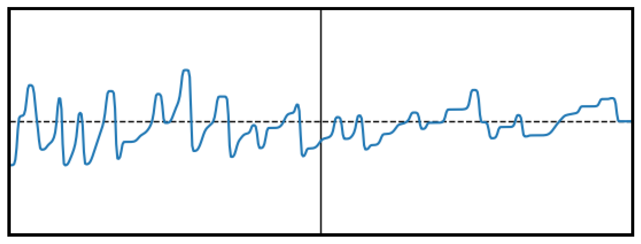
The situation is summed up in Figure 19. When laterally excited, the surface of the fluid sloshes back and forth in the tank, generating complex patterns at the fluid surface, as shown in Figure 20. When the excitation stops, a relaxation phase is observed, usually leaving a single wavefront traveling back and forth in the tank until it dissipates entirely. Due to its simplicity, model (24) does not allow wave breaking nor the formation of drops on the sides of the domain.
3.6.2. Discretization
3.6.3. Environment
The control of system (24) is performed through the cart acceleration term . The system is first set in motion during time units using a sinusoid-based signal as follows:
The resulting fields are stored in a file for simplicity and loaded at the beginning of each episode. By default, the length of the cart is , the spatial discretization corresponds to 100 finite-volume cells per unit of length, and the numerical time-step is time units. The actions provided to the environment, which are expected to be in , are then scaled by an ad hoc non-dimensional amplitude factor . The interpolation between successive actions is identical to (8), with time units and time units. The total episode time is fixed to 10 time units, corresponding to 200 actions. The observations provided to the agent are the heights collected on the entire domain. To limit the size of the resulting vector, it is downsampled by a factor of 2. Finally, the reward signal is defined as:
where is the 2-norm, and . The factor allows us to obtain comparable reward values for variable discretization levels.
3.6.4. Results
The environment described in the previous section is referred to as sloshing-v0, and its default parameters are provided in Table 8. In this section, we note that the critic learning rate of the ppo agent is reduced to compared to the default hyperparameters of Table 2. For the training, we set , , , and k. The score curves are presented in Figure 21, while the time evolutions of the controlled versus uncontrolled fluid level are shown in Figure 22. As can be observed, the agent manages to roughly cut the uncontrolled reward in half by suppressing the back-and-forth wavefront using large actuations in the early stages of control, after which the control amplitude drops significantly.
3.7. Vortex
3.7.1. Physics
We consider the resolution of a dynamical system modeling the non-linear, vortex-induced vibrations of a rigid circular cylinder. The flow motion is governed by the incompressible Navier–Stokes equations, whereas the cylinder motion is a simple translation governed by a linear mass–damper–spring equation affected by the fluid loading. This is modeled by coupled amplitude equations derived in [11,35] after dominant balance arguments as follows:
where A and Y are unknown slow, time-varying, complex amplitudes modeling, respectively, the flow disturbances and the cylinder center of mass, is the Reynolds number, is the threshold of instability of the steady cylinder, is the frequency of the marginally stable eigenmode classically computed from the flow past a fixed cylinder [36], is the dimensionless natural frequency of the cylinder in vacuum, is the structural damping coefficient, and is the ratio of the solid to the fluid densities. The coefficients , , , and in (30) are analytically computable from an asymptotic analysis of the coupled flow–cylinder system, their numerical value being taken from [35] as:
The ability of the model to reproduce the physics of vortex-induced vibrations has been assessed from the study of the non-linear limit cycles, i.e., the periodic, synchronized orbits reached by the system in large periods of time whose analytical expressions are reported in [35]. Of particular importance is the simultaneous existence of multiple stable cycles (either a single limit cycle or three over specific ranges of frequencies), which is shown to trigger a complex hysteretic behavior in the lock-in regime. Since all limit cycle solutions are periodic, the mean mechanical energy averaged over a period is zero, and the mean work received from the fluctuating lift force is entirely dissipated by structural damping. As discussed in [35], it follows that the leading-order mean dissipated energy is a simple quadratic function of the displacement amplitude, meaning that only the upper limit cycle (the one limit cycle yielding the largest displacement amplitude) is of practical interest for the energy extraction problem, that is, in cases where one seeks to leverage such vortex-induced vibrations to generate electrical energy, for instance, by having the oscillation of the cylinder periodically displace a magnet within a coil.
In essence, it can be inferred that there must exist an optimal structural parameter setting for which the dissipated energy is maximum. On the one hand, the flow–cylinder system must be synchronized for the cylinder displacement amplitude to be large. On the other hand, the energy tends to zero in the limit , where the work received from the lift force is limited by the low amplitude of the displacement, and in the limit , where the displacement is self-limited. As evidenced in [11], the problem shown is that the optimum lies at the edge of a discontinuity, corresponding to parameter settings where the system undergoes a transition from a hysteretic to a non-hysteretic regime. This has important consequences for the application since small inaccuracies in the structural parameters of small external flow disturbances may tip the system outside the hysteresis zone and lead to convergence to cycles of lower energy, resulting in a dramatic drop in the harnessed energy.
3.7.2. Discretization
3.7.3. Environment
The proposed environment is re-implemented based on the original work of [11], where the goal was to maximize the cylinder displacement and bypass the existence of low-energy cycles. This is achieved by adding a proportional feedback control in the structure equation, assuming that the state of the system is accessed through measurements of the flow disturbances’ position and that an actuator applies a control velocity at the surface of the cylinder as follows:
where k is the gain and the phase shift between the measure and the action. The actions provided to the environment, which are expected to be in , are rescaled to for the module and for the phase. The action time-step is set to time units, a full episode lasting 400 time units, corresponding to 800 actions. The observations are the complex variables A and Y as well as their time derivatives, leading to an observation vector of size 8. The reward at each time-step is computed as:
where the leftmost term is the mean dissipated energy and is thus associated with performance, the rightmost term estimates the mean kinetic energy expended by the actuator over a limit cycle period and is thus associated with cost, and w is a weighting coefficient set empirically to 50 (a value found to be large enough for cost considerations to impact the optimization procedure but not so large as to dominate the reward signal, in which case, actuating is meaningless). Each episode begins using the same initial condition, , which, in the absence of control, leads to convergence to a low limit cycle, for which the score is equal to .
3.7.4. Results
The environment described in the previous section is referred to as vortex-v0, and its default parameters are provided in Table 9. In this section, we note that the critic learning rate of the ppo agent is reduced to compared to the default hyperparameters of Table 2. For the training, we set , , , and k. The score curves are presented in Figure 23, while the time evolutions of the controlled versus uncontrolled fluid level are shown in Figure 24. As can be observed, the agent manages to lock in a high limit cycle, with a final score more than 3 orders of magnitude larger than that of the uncontrolled low limit cycle, and twice as large as that of the uncontrolled high limit cycle (whose score computed using is ).
4. Conclusions and Availability
In the present work, seven fluid dynamics environments are proposed, each of them being representative of a specific physical phenomenon. We observed that the performance ranking usually observed in standard benchmarks such as gym and mujoco (i.e., off-policy methods usually significantly outperform on-policy approaches) is not necessarily valid in the context of flow control environments.
The environments are implemented in a modular way, following the structure of the gym library to allow for a seamless integration with existing code. Optimizations have been run on each of the cases, and the results have been commented on in each of the respective sections. The sources of the present work are made open in the following repository: https://github.com/jviquerat/beacon (accessed on 26 February 2024).
While the present version of the library presents a modest variety of phenomena and control types, its purpose is to grow with new cases proposed by the community, within the constraints detailed in Section 2. To this end, issues and pull requests are accepted in the library repository. With the present work, we hope to provide a solid foundation for the development of a community-driven library of fluid dynamics environments and to foster the development of new control strategies for fluid dynamics.
Author Contributions
Conceptualization, J.V. and E.H.; Formal analysis, J.V., P.M. and P.J.-R.; Software, J.V., P.M. and P.J.-R.; Validation, J.V.; Visualization, J.V.; Writing, J.V., P.M., P.J.-R. and E.H.; Funding acquisition, E.H. All authors have read and agreed to the published version of the manuscript.
Funding
Funded/co-funded by the European Union (ERC, CURE, 101045042). Views and opinions expressed are, however, those of the authors only and do not necessarily reflect those of the European Union or the European Research Council; neither the European Union nor the granting authority can be held responsible for them.
Institutional Review Board Statement
Not applicable.
Informed Consent Statement
Not applicable.
Data Availability Statement
The data presented in this study are available at https://github.com/jviquerat/beacon.
Conflicts of Interest
The authors declare no conflict of interest.
Appendix A. Implementations Benchmarks
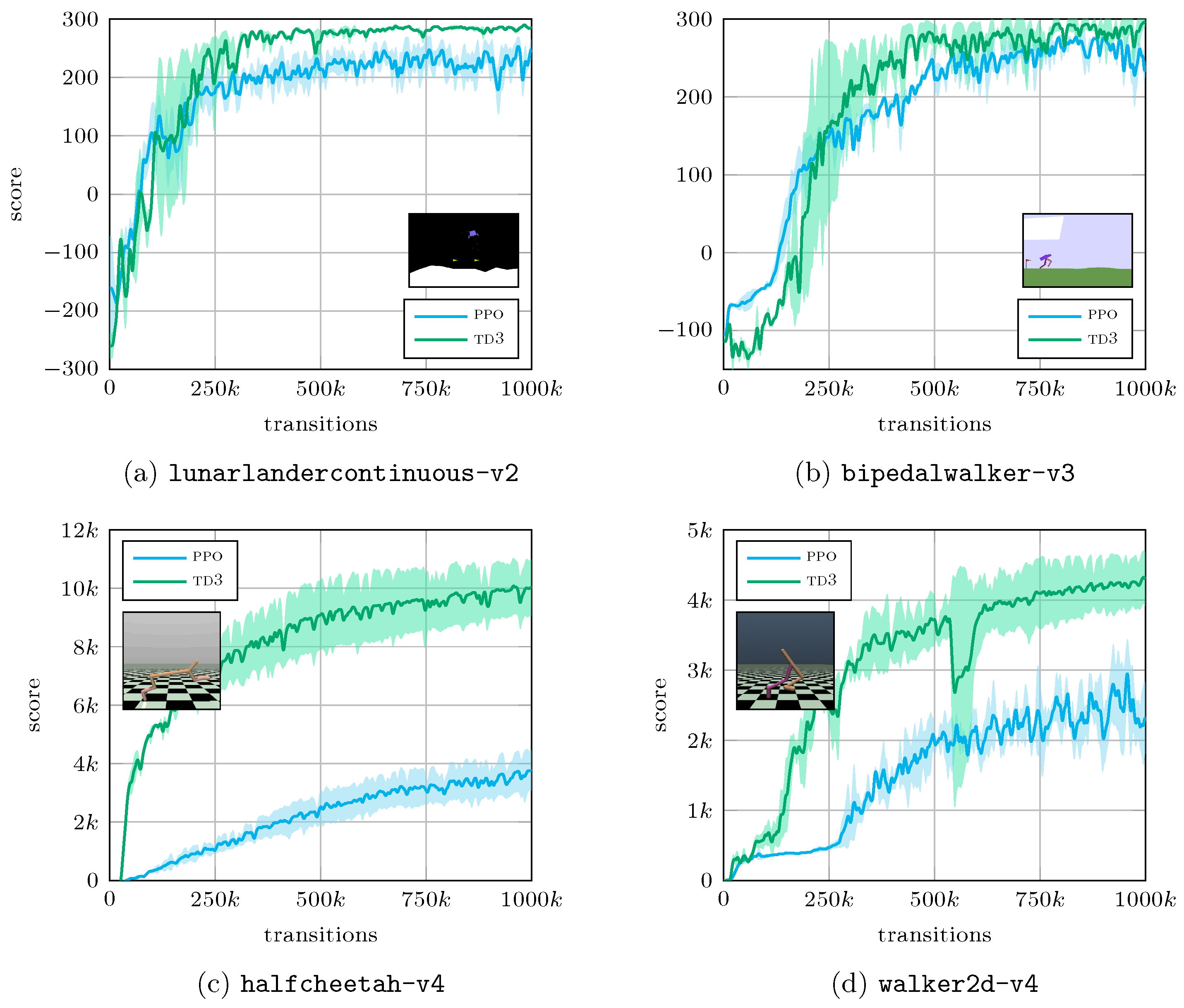
This section is dedicated to the evaluation of the in-house ppo and td3 algorithms on standard benchmarks. In this regard, we selected two cases from the gym library, and two cases from the mujoco library. Results are presented in Figure A1. The implementations used to solve the beacon benchmark cases compare favourably with reference implementations.
Figure A1.
Performance benchmark of our in-house ppo and td3 algorithms on standard gym and mujoco environments. These results compare favourably with reference implementations [37].
Figure A1.
Performance benchmark of our in-house ppo and td3 algorithms on standard gym and mujoco environments. These results compare favourably with reference implementations [37].

References
- Wang, Y.Z.; Mei, Y.F.; Aubry, N.; Chen, Z.; Wu, P.; Wu, W.T. Deep reinforcement learning based synthetic jet control on disturbed flow over airfoil. Phys. Fluids 2022, 34, 033606. [Google Scholar] [CrossRef]
- Novati, G.; Verma, S.; Alexeev, D.; Rossinelli, D.; Van Rees, W.M.; Koumoutsakos, P. Synchronisation through learning for two self-propelled swimmers. Bioinspir. Biomim. 2017, 12, 036001. [Google Scholar] [CrossRef] [PubMed]
- Beintema, G.; Corbetta, A.; Biferale, L.; Toschi, F. Controlling rayleigh–bénard convection via reinforcement learning. J. Turbul. 2020, 21, 585–605. [Google Scholar] [CrossRef]
- Viquerat, J.; Meliga, P.; Larcher, A.; Hachem, E. A review on deep reinforcement learning for fluid mechanics: An update. Phys. Fluids 2022, 34, 111301. [Google Scholar] [CrossRef]
- Andrychowicz, M.; Raichuk, A.; Stańczyk, P.; Orsini, M.; Girgin, S.; Marinier, R.; Hussenot, L.; Geist, M.; Pietquin, O.; Michalski, M.; et al. What matters in on-policy reinforcement learning? A large-scale empirical study. arXiv 2020, arXiv:2006.05990. [Google Scholar]
- Todorov, E.; Erez, T.; Tassa, Y. Mujoco: A physics engine for model-based control. In Proceedings of the 2012 IEEE/RSJ International Conference on Intelligent Robots and Systems, Vilamoura-Algarve, Portugal, 7–12 October 2012; IEEE: Piscataway, NJ, USA, 2012; pp. 5026–5033. [Google Scholar]
- Bellemare, M.G.; Naddaf, Y.; Veness, J.; Bowling, M. The arcade learning environment: An evaluation platform for general agents. J. Artif. Intell. Res. 2013, 47, 253–279. [Google Scholar] [CrossRef]
- Brockman, G.; Cheung, V.; Pettersson, L.; Schneider, J.; Schulman, J.; Tang, J.; Zaremba, W. Openai gym. arXiv 2016, arXiv:1606.01540. [Google Scholar]
- Rabault, J.; Kuhnle, A. Accelerating deep reinforcement learning strategies of flow control through a multi-environment approach. Phys. Fluids 2019, 31, 094105. [Google Scholar] [CrossRef]
- Viquerat, J.; Hachem, E. Parallel bootstrap-based on-policy deep reinforcement learning for continuous fluid flow control applications. Fluids 2023, 8, 208. [Google Scholar] [CrossRef]
- Meliga, P.; Chomaz, J.M.; Gallaire, F. Extracting energy from a flow: An asymptotic approach using vortex-induced vibrations and feedback control. J. Fluids Struct. 2011, 27, 861–874. [Google Scholar] [CrossRef]
- Belus, V.; Rabault, J.; Viquerat, J.; Che, Z.; Hachem, E.; Reglade, U. Exploiting locality and translational invariance to design effective deep reinforcement learning control of the 1-dimensional unstable falling liquid film. AIP Adv. 2019, 9, 125014. [Google Scholar] [CrossRef]
- Lam, S.K.; Pitrou, A.; Seibert, S. Numba: A llvm-based python jit compiler. In Proceedings of the Second Workshop on the LLVM Compiler Infrastructure in HPC, Austin, TX, USA, 15 November 2015. [Google Scholar]
- Harris, C.R.; Millman, K.J.; Van Der Walt, S.J.; Gommers, R.; Virtanen, P.; Cournapeau, D.; Wieser, E.; Taylor, J.; Berg, S.; Smith, N.J.; et al. Array programming with NumPy. Nature 2020, 585, 357–362. [Google Scholar] [CrossRef] [PubMed]
- Hunter, J.D. Matplotlib: A 2D graphics environment. Comput. Sci. Eng. 2007, 9, 90–95. [Google Scholar] [CrossRef]
- Schulman, J.; Wolski, F.; Dhariwal, P.; Radford, A.; Klimov, O. Proximal policy optimization algorithms. arXiv 2017, arXiv:1707.06347. [Google Scholar]
- Mnih, V.; Kavukcuoglu, K.; Silver, D.; Rusu, A.A.; Veness, J.; Bellemare, M.G.; Graves, A.; Riedmiller, M.; Fidjeland, A.K.; Ostrovski, G.; et al. Human-level control through deep reinforcement learning. Nature 2015, 518, 529–533. [Google Scholar] [CrossRef] [PubMed]
- Fujimoto, S.; Hoof, H.; Meger, D. Addressing function approximation error in actor-critic methods. arXiv 2018, arXiv:1802.09477. [Google Scholar]
- Kapitza, P.L. Wave flow of a thin viscous fluid layers. Zhurnal Eksperimental’Noi Teor. Fiz. 1948, 18, 3–18. [Google Scholar]
- Shkadov, V.Y. Wave flow regimes of a thin layer of viscous fluid subject to gravity. Fluid Dyn. 1967, 2, 29–34. [Google Scholar] [CrossRef]
- Lavalle, G. Integral Modeling of Liquid Films Sheared by a Gas Flow. Ph.D. Thesis, ISAE—Institut Supérieur de l’Aéronautique et de l’Espace, Toulouse, France, 2014. [Google Scholar]
- Chang, H.C.; Demekhin, E.A.; Saprikin, S.S. Noise-driven wave transitions on a vertically falling film. J. Fluid Mech. 2002, 462, 255–283. [Google Scholar] [CrossRef]
- Chang, H.-H.; Demekhin, E.A. Complex Wave Dynamics on Thin Films; Elsevier: Amsterdam, The Netherlands, 2002. [Google Scholar]
- Koulago, A.E.; Parséghian, D. A propos d’une équation de la dynamique ondulatoire dans les films liquides. J. Phys. III 1995, 5, 309–312. [Google Scholar] [CrossRef]
- Boivin, S.; Cayré, F.; Herard, J.M. A finite volume method to solve the navier—Stokes equations for incompressible flows on unstructured meshes. Int. J. Therm. Sci. 2000, 39, 806–825. [Google Scholar] [CrossRef]
- Ouertatani, N.; Cheikh, N.B.; Beya, B.B.; Lili, T. Numerical simulation of two-dimensional rayleigh—Bénard convection in an enclosure. Comptes Rendus Mécanique 2008, 336, 464–470. [Google Scholar] [CrossRef]
- Saltzman, B. Finite amplitude free convection as an initial value problem. J. Atmos. Sci. 1962, 19, 329–341. [Google Scholar] [CrossRef]
- Lorenz, E.N. Deterministic nonperiodic flow. J. Atmos. Sci. 1963, 20, 130–141. [Google Scholar] [CrossRef]
- Carpenter, M.H.; Kennedy, C.A. Fourth-Order 2n-Storage Runge-Kutta Schemes; Technical Report; National Aeronautics and Space Administration: Washington, DC, USA, 1994. [Google Scholar]
- Bateman, H. Some recent researches on the motion of fluids. Mon. Weather. Rev. 1915, 43, 163–170. [Google Scholar] [CrossRef]
- Burgers, J.M. A mathematical model illustrating the theory of turbulence. Adv. Appl. Mech. 1948, 1, 171–199. [Google Scholar]
- Saint-Venant, A.J.C. Théorie du mouvement non permanent des eaux, avec application aux crues des rivières et a l’introduction de marées dans leurs lits. Comptes Rendus Séances Académie Sci. 1871, 73, 148–154. [Google Scholar]
- Berger, T.; Puche, M.; Schwenninger, F.L. Funnel control for a moving water tank. Automatica 2022, 135, 109999. [Google Scholar] [CrossRef]
- Cordier, S.; Darboux, F.; Delestre, O.; James, F. Etude D’un Modèle de Ruissellement 1D; Technical Report; University of Orléans: Orléans, France; INRA: Paris, France, 2007. [Google Scholar]
- Meliga, P.; Chomaz, J.M. An asymptotic expansion for the vortex-induced vibrations of a circular cylinder. J. Fluid Mech. 2011, 671, 137–167. [Google Scholar] [CrossRef]
- Barkley, D. Linear analysis of the cylinder wake mean flow. Europhys. Lett. 2006, 75, 750. [Google Scholar] [CrossRef]
- Achiam, J. Spinning up in Deep Reinforcement Learning. 2018. Available online: https://spinningup.openai.com/en/latest/index.html (accessed on 16 April 2024).
Figure 1.
Example of developed flow for the Shkadov equations with . Three regions can be identified: a first region where the instability grows from a white noise (blue), a second region with pseudo-periodic waves (orange), and a third region with non-periodic, pulse-like waves (green).
Figure 1.
Example of developed flow for the Shkadov equations with . Three regions can be identified: a first region where the instability grows from a white noise (blue), a second region with pseudo-periodic waves (orange), and a third region with non-periodic, pulse-like waves (green).

Figure 2.
Score curves for the shkadov-v0 environment in different configurations. (a) comparison of score curves for ppo and td3 algorithms in the default configuration using 5 jets. (b) comparison of different number of jets using the ppo algorithm. For each curve, we plot the average (solid color) and the standard deviation (shaded color) obtained from different runs. The dashed line indicates the reward obtained for the uncontrolled environment.

Figure 3.
Evolution of the flow under control of the agent using 5 jets. The jets strengths are represented in the bottom rectangle (red means positive amplitude, blue means negative amplitude). The horizontal and vertical axes are the same as in Figure 1.
Figure 3.
Evolution of the flow under control of the agent using 5 jets. The jets strengths are represented in the bottom rectangle (red means positive amplitude, blue means negative amplitude). The horizontal and vertical axes are the same as in Figure 1.

Figure 4.
Temperature and velocity profiles for the uncontrolled Rayleigh convection cell with , , , and . (Left) The adimensional temperature ranges from 0 (deep blue) to 1 (deep red). (Right) The non-dimensional velocity amplitude ranges from 0 (deep blue) to 1 (deep red).
Figure 4.
Temperature and velocity profiles for the uncontrolled Rayleigh convection cell with , , , and . (Left) The adimensional temperature ranges from 0 (deep blue) to 1 (deep red). (Right) The non-dimensional velocity amplitude ranges from 0 (deep blue) to 1 (deep red).

Figure 5.
Observation probes and actions imposition for the rayleigh-v0 environment. The observations are collected at the probes regularly positioned in the domain, while the actions are imposed as piecewise constant temperature boundary conditions on the bottom plate with an average value equal to . Non-dimensional temperature color scale is the same as that of Figure 4.

Figure 6.
Score curves obtained using the ppo and the td3 algorithms to solve the rayleigh-v0 environment. The dashed line indicates the reward obtained for the uncontrolled environment.
Figure 6.
Score curves obtained using the ppo and the td3 algorithms to solve the rayleigh-v0 environment. The dashed line indicates the reward obtained for the uncontrolled environment.

Figure 7.
Evolution of the instantaneous Nusselt number during an episode of the rayleigh-v0 environment with and without control. The agent totally disables the convection, leading to a final Nusselt number equal to 1.
Figure 7.
Evolution of the instantaneous Nusselt number during an episode of the rayleigh-v0 environment with and without control. The agent totally disables the convection, leading to a final Nusselt number equal to 1.

Figure 8.
Evolution of the convection cell under control of the agent during the first steps of the environment. After a strong initial forcing, the agent establishes a pattern of alternating hot and cold actions that leads to a stationary configuration with . The control of the agent remains the same for the rest of the environment. The local temperature variations due to the control of the agent are represented in the bottom rectangle (red means positive amplitude, blue means negative amplitude). Non-dimensional temperature color scale is the same as that of Figure 4.

Figure 9.
Evolution of the concentration in time with constant boundary conditions . The non-dimensional concentration ranges from 0 (deep blue) to 1 (deep red).
Figure 9.
Evolution of the concentration in time with constant boundary conditions . The non-dimensional concentration ranges from 0 (deep blue) to 1 (deep red).

Figure 10.
Score curves obtained using the ppo and the dqn algorithms to solve the mixing-v0 environment. The dashed line indicates the reward obtained for the uncontrolled environment.
Figure 10.
Score curves obtained using the ppo and the dqn algorithms to solve the mixing-v0 environment. The dashed line indicates the reward obtained for the uncontrolled environment.

Figure 11.
Evolution of the mixing cell under control of the agent. The instantaneous controls are indicated with the four colored bars. Non-dimensional concentration color scale is the same as that of Figure 9.
Figure 11.
Evolution of the mixing cell under control of the agent. The instantaneous controls are indicated with the four colored bars. Non-dimensional concentration color scale is the same as that of Figure 9.

Figure 12.
Control-free evolution of the Lorenz system. The attractor’s trajectory forms a distinctive, butterfly-like shape that consists of two large, symmetrically arranged lobes.
Figure 12.
Control-free evolution of the Lorenz system. The attractor’s trajectory forms a distinctive, butterfly-like shape that consists of two large, symmetrically arranged lobes.

Figure 13.
Score curves for the ppo and dqn algorithms when solving the lorenz-v0 environment. The dashed line indicates the reward obtained in the uncontrolled case.
Figure 13.
Score curves for the ppo and dqn algorithms when solving the lorenz-v0 environment. The dashed line indicates the reward obtained in the uncontrolled case.

Figure 14.
Controlled versus uncontrolled time evolution of the x parameter. The red dot corresponds to the typical control peak that precedes the locking of the system, also observed in [3].
Figure 14.
Controlled versus uncontrolled time evolution of the x parameter. The red dot corresponds to the typical control peak that precedes the locking of the system, also observed in [3].

Figure 15.
Evolution of the controlled Lorenz system using the ppo algorithm. The instantaneous control value is indicated at the bottom by the colored bar (blue is for , red is for ).
Figure 15.
Evolution of the controlled Lorenz system using the ppo algorithm. The instantaneous control value is indicated at the bottom by the colored bar (blue is for , red is for ).

Figure 16.
Uncontrolled solution of the Burgers equation with uniform random noise excitation at the inlet. The horizontal axis represents the x coordinate, with the vertical bar indicating the position of the controller. The vertical axis represents the velocity of the fluid.
Figure 16.
Uncontrolled solution of the Burgers equation with uniform random noise excitation at the inlet. The horizontal axis represents the x coordinate, with the vertical bar indicating the position of the controller. The vertical axis represents the velocity of the fluid.

Figure 17.
Score curves for the ppo and the td3 algorithms when solving the burgers-v0 environment. The dashed line indicates the reward obtained for the uncontrolled case.
Figure 17.
Score curves for the ppo and the td3 algorithms when solving the burgers-v0 environment. The dashed line indicates the reward obtained for the uncontrolled case.

Figure 18.
Evolution of the controlled burgers system using the ppo algorithm. The instantaneous control value is indicated at the bottom by the colored bar (blue is for negative actuations, while red is for positive ones). The axes are the same as in Figure 16.
Figure 18.
Evolution of the controlled burgers system using the ppo algorithm. The instantaneous control value is indicated at the bottom by the colored bar (blue is for negative actuations, while red is for positive ones). The axes are the same as in Figure 16.

Figure 19.
Configuration of the sloshing tank. The fluid flow is determined by the fluid height and by its mass flow rate . The movement of the tank is controlled by its acceleration .
Figure 19.
Configuration of the sloshing tank. The fluid flow is determined by the fluid height and by its mass flow rate . The movement of the tank is controlled by its acceleration .

Figure 20.
Examples of fluid surface during the excitation phase (left) and the relaxation phase (right). The horizontal axis represents the x coordinate, while the vertical axis represents the height of the fluid. The horizontal line indicates the height of the fluid at rest ().
Figure 20.
Examples of fluid surface during the excitation phase (left) and the relaxation phase (right). The horizontal axis represents the x coordinate, while the vertical axis represents the height of the fluid. The horizontal line indicates the height of the fluid at rest ().

Figure 21.
Score curves for the sloshing-v0 environment using the ppo and the td3 algorithms. The dashed line indicates the reward obtained for the uncontrolled environment.
Figure 21.
Score curves for the sloshing-v0 environment using the ppo and the td3 algorithms. The dashed line indicates the reward obtained for the uncontrolled environment.

Figure 22.
Evolution of the fluid surface with (left) and without (right) agent control. The control amplitude and direction are represented using the rectangle at the bottom (red means positive, blue means negative). The axes are the same as in Figure 20.
Figure 22.
Evolution of the fluid surface with (left) and without (right) agent control. The control amplitude and direction are represented using the rectangle at the bottom (red means positive, blue means negative). The axes are the same as in Figure 20.

Figure 23.
Score curves for the vortex-v0 environment using the ppo and the td3 algorithms. The uncontrolled environment obtains a score of when locking in on the low limit cycle.
Figure 23.
Score curves for the vortex-v0 environment using the ppo and the td3 algorithms. The uncontrolled environment obtains a score of when locking in on the low limit cycle.

Figure 24.
Evolution of the phase portrait of the controlled vortex system using the ppo algorithm. The instantaneous control values are indicated at the bottom by the colored bars (blue means negative control value, red means positive control value).
Figure 24.
Evolution of the phase portrait of the controlled vortex system using the ppo algorithm. The instantaneous control values are indicated at the bottom by the colored bars (blue means negative control value, red means positive control value).


Table 1.
Overview of the different environments in their default configurations.
| Env. Name | Action Dim. | CPU Requirements | Problem Type | Control Type |
|---|---|---|---|---|
| shkadov-v0 | 5 | moderate | continuous | continuous |
| rayleigh-v0 | 10 | high | continuous | continuous |
| mixing-v0 | 4 | high | episodic | discrete |
| lorenz-v0 | 1 | moderate | continuous | discrete |
| burgers-v0 | 1 | low | continuous | continuous |
| sloshing-v0 | 1 | low | episodic | continuous |
| vortex-v0 | 2 | moderate | continuous | continuous |
Table 2.
Default parameters used for the ppo agent.
| – | agent type | ppo-clip |
| discount factor | 0.99 | |
| actor learning rate | 5 × 10⁻⁴ | |
| critic learning rate | 5 × 10⁻³ | |
| – | optimizer | adam |
| – | weights initialization | orthogonal |
| – | activation (actor hidden layers) | tanh |
| – | activation (actor final layer, continous) | tanh, sigmoid |
| – | activation (actor final layer, discrete) | softmax |
| – | activation (critic hidden layers) | relu |
| – | activation (critic final layer) | linear |
| PPO clip value | 0.2 | |
| entropy bonus | 0.01 | |
| g | gradient clipping value | 0.1 |
| – | actor network | |
| – | critic network | |
| – | observation normalization | yes |
| – | observation clipping | no |
| – | advantage type | GAE |
| bias–variance trade-off | 0.99 | |
| – | advantage normalization | yes |
| no. of transitions per update | env. specific | |
| no. of minibatches per update | env. specific | |
| no. of epochs per update | env. specific | |
| total no. of transitions per training | env. specific | |
| total no. of averaged trainings | 5 |
Table 3.
Default parameters for shkadov-v0.
| L0 | base length of domain | 150 |
| n_jets | number of jets | 5 |
| jet_pos | position of first jet | 150 |
| jet_space | spacing between jets | 10 |
| delta | physical parameter (2) |
Table 4.
Default parameters used for rayleigh-v0.
| L | length of the domain | 1 |
| H | height of the domain | 1 |
| n_sgts | number of control segments | 10 |
| ra | Rayleigh number |
Table 5.
Default parameters used for mixing-v0.
| L | length of the domain | 1 |
| H | height of the domain | 1 |
| re | Reynolds number | |
| pe | Péclet number | |
| side | initial side length of concentration patch | |
| c0 | initial concentration | 1 |
Table 6.
Default parameters used for lorenz-v0.
| sigma | Lorenz parameter | 10 |
| rho | Lorenz parameter | 28 |
| beta | Lorenz parameter |
Table 7.
Default parameters used for burgers-v0.
| L | domain length | 2 |
| u_target | target value | |
| sigma | inlet noise level | |
| amp | control amplitude | 10 |
| ctrl_pos | control position | 1 |
Table 8.
Default parameters used for sloshing-v0.
| L | length of the tank | |
| amp | amplitude of the control | 5 |
| alpha | control penalization | |
| g | gravity acceleration |
Table 9.
Default parameters used for vortex-v0.
| re | Reynolds number | 50 |
| w | control penalization | 50 |
Disclaimer/Publisher’s Note: The statements, opinions and data contained in all publications are solely those of the individual author(s) and contributor(s) and not of MDPI and/or the editor(s). MDPI and/or the editor(s) disclaim responsibility for any injury to people or property resulting from any ideas, methods, instructions or products referred to in the content. |
© 2024 by the authors. Licensee MDPI, Basel, Switzerland. This article is an open access article distributed under the terms and conditions of the Creative Commons Attribution (CC BY) license (https://creativecommons.org/licenses/by/4.0/).
Share and Cite
MDPI and ACS Style
Viquerat, J.; Meliga, P.; Jeken-Rico, P.; Hachem, E. Beacon, a Lightweight Deep Reinforcement Learning Benchmark Library for Flow Control. Appl. Sci. 2024, 14, 3561. https://doi.org/10.3390/app14093561
AMA Style
Viquerat J, Meliga P, Jeken-Rico P, Hachem E. Beacon, a Lightweight Deep Reinforcement Learning Benchmark Library for Flow Control. Applied Sciences. 2024; 14(9):3561. https://doi.org/10.3390/app14093561
Chicago/Turabian StyleViquerat, Jonathan, Philippe Meliga, Pablo Jeken-Rico, and Elie Hachem. 2024. "Beacon, a Lightweight Deep Reinforcement Learning Benchmark Library for Flow Control" Applied Sciences 14, no. 9: 3561. https://doi.org/10.3390/app14093561
Note that from the first issue of 2016, this journal uses article numbers instead of page numbers. See further details here.