
Radar Error Correction Method Based on Improved Sparrow Search Algorithm

College of Weapons Engineering, Naval University of Engineering, Wuhan 430033, China
*
Author to whom correspondence should be addressed.
Appl. Sci. 2024, 14(9), 3714; https://doi.org/10.3390/app14093714
Submission received: 18 March 2024
/
Revised: 22 April 2024
/
Accepted: 22 April 2024
/
Published: 26 April 2024
(This article belongs to the Topic Radar Signal and Data Processing with Applications)
Abstract
:Aiming at the problem of the limited application range and low accuracy of existing radar calibration methods, this paper studies the radar calibration method based on cooperative targets, and establishes the integrated radar measurement error model. Then, the improved sparrow search algorithm (ISSA) is used to estimate the systematic error, so as to avoid the loss of partial accuracy caused by the process of approximating the nonlinear equation to the linear equation, thus improving the radar calibration effect. The sparrow search algorithm (SSA) is improved through integrating various strategies, and the convergence speed and stability of the algorithm are also improved. The simulation results show that the ISSA can solve radar systematic errors more accurately than the generalized least square method, Kalman filter, and SSA. It takes less time the than SSA and has a certain stability and real-time performance. The radar measurement error after correction is obviously smaller than that before correction, indicating that the proposed method is feasible and effective.
1. Introduction
Radar is the main means of the monitoring of and early warnings for non-cooperative targets at sea [1,2]. The modern radar represented by phased arrays can detect and track multiple targets, such as ships, aircrafts, and missiles at the same time because of its fast beam control speed [3,4]. However, due to the influence of mechanical structure deflection, installation platform tilt, the aging of internal electrical components, external electromagnetic interference, and other factors [5], radar measurements often have various forms of error (as shown in Figure 1), and the maximum error can even reach the magnitude of kilometers [6], therefore it is necessary to calibrate the radar regularly. In previous studies, radar observation errors were usually divided into random errors and systematic errors [7]. The random error can be eliminated using a filtering algorithm, and the impact on the subsequent measurement results is relatively small [8]. The systematic error is the fixed deviation generated by the characteristics of the radar system itself and the interaction with the external environment, which cannot be removed through the use of filtering, and needs to be estimated in advance to then be compensated for. This process is called radar calibration.
Traditional land-based radar calibration usually uses fixed targets with known positions on the ground or establishes registration models, and solves them through measuring the same target in the common observation area of multiple radars [9,10,11,12]. The calibration range of this method is limited, and it cannot be applied in the far sea area. To solve this problem, Luo Jun and Pan Shao-Ren, respectively, proposed the idea of using AIS information to calibrate radars [13,14]. However, this idea requires that the systematic error of the same radar is basically constant in a certain space–time range, and that the detection accuracy of the different targets is identical or similar. In this regard, references [8,15,16] analyzed a large number of measured data and found that the multi-target error samples in the radar coverage area were relatively concentrated, showing the characteristics of correlation and normalizing distribution statistically; therefore, the systematic error could be regarded as a constant value within a certain time and region. The studies in references [17,18] show that radar systematic errors are jointly determined by hardware design, manufacturing process, installation conditions, operation parameter setting, and environmental factors, while it does not depend on the specific attributes and states of the measured targets; that is, it will have a consistent impact on almost all targets’ measurements. Therefore, it is feasible to use the self-reported position information of the moving target to carry out radar calibration. The method is favored by many experts and scholars because of its convenient and flexible selection of calibration sources and high positioning accuracy. Professor Dong’s team took the AIS data as the true value in order to analyze the error distribution characteristics of the radar system, and they solved the problem of the low reliability of the error estimates under the assumption of uniform distribution through the use of the method of partition processing, but it did not establish a universal error model for the measured target, which was limited by the accumulation of error data in the database [15,19,20]. Considering that the error calibration of the three-coordinate radar needs to include three-dimensional position information, Wu proposed a real-time radar error correction algorithm based on ADS-B data, derived the error observation model, and used Kalman filtering (KF) algorithm to solve it. It is more stable than the algorithm that uses the mean error as the systematic error to complete the calibration [21]. Academician He’s team derived a combined system error model, taking the ADS-B system delay into account, and solved it using generalized least squares (GLS) [22], both of which require the linearization of the nonlinear model to be solved. Li P proposed the use of the SICP algorithm to estimate the radar systematic error. This method does not need to establish the radar measurement error model, and only realizes error estimation through the translation transformation matrix between two tracks. However, this method is sensitive to measurement noise and too dependent on data correlation results [23]. Zhang Tao proposed a radar systematic error estimation scheme, based on the probability hypothesis density (PHD). Although it can achieve target error estimation without prior correlation information, it also has an approximation to nonlinear equations, meaning the radar calibration effect was affected [24].
To solve the above problems, this paper first studies the radar calibration method, based on the cooperative target, and establishes the integrated radar measurement error model by referring to the position information of the cooperative aircraft in the radar range. On this basis, an error estimation method based on the improved sparrow search algorithm (ISSA) is proposed to transform the nonlinear model solving problem into the multidimensional multi-peak optimization problem, so as to avoid the introduction of deviation in the linearization process of the nonlinear system. At the same time, a variety of strategies are used to improve the convergence speed of the sparrow search algorithm (SSA), so that the radar systematic error estimation can be both accurate and in real time, so as to improve the radar calibration effect and the target track accuracy.
2. Radar Measurement Error Model
The key of radar calibration is to estimate the systematic error accurately. This paper deduces the radar observation error model from the radar calibration principle based on the cooperative target.
The method of radar calibration, based on the cooperative target, consists of detecting the cooperative target, which is equipped with a global navigation satellite system (GNSS) and can transmit its position to us in real time through a data link (the cooperative targets mentioned above all refer to cooperative aircraft in this paper), and use it as the reference source. After the position data of the reference source measured by the GNSS are associated with the radar measurement data, time registration, and coordinate transformation, the difference between the two is used to estimate the radar systematic error, so as to achieve radar calibration. The basic principle is shown in Figure 2.
The correlation between the GNSS and radar measurement data is the primary link of radar calibration, which can be realized by the nearest neighbor (NN) association algorithm [25], joint probability data association (JPDA) [26], and other algorithms. There are many relevant studies and the technology is relatively mature, so this paper will not go into detail.
Through time registration, the GNSS information received can be extrapolated in order to keep time synchronization with the radar positioning data. However, there is a delay in data link communication, and the sending time of the GNSS positioning data is deviated from the radar measurement time (this deviation is referred to as the communication delay in the paper), during which the aircraft will still fly forward for a certain distance. Due to the high speed of the aircraft when moving, the position error caused by the communication delay cannot be ignored. The GNSS data transmission period of the cooperation target is set as TG, the radar measurement period as TR, the GNSS data transmission time is successively the radar measurement time is , and the time deviation between the two is, in turn, . The following relationships can be obtained:
Through smoothing and interpolation algorithms [27,28], the position-sending period of the cooperative target is reconstructed so that TG = TR, which can be obtained via ; that is, the communication delay is a constant value . After estimating this value, the position deviation caused by the communication delay can be corrected via combining it with the aircraft speed.
The cooperative target points obtained by the GNSS are represented by the longitude, latitude, and altitude in the WGS-84 coordinate system, while the radar measurement track is in the radar-centered polar coordinate system, and the two must be unified. Because the common least square method and Kalman filter are the linear estimation algorithms, they are transformed to the Cartesian coordinate system. In this paper, the Earth-centered, Earth-fixed (ECEF) coordinate system is used as a unified coordinate system, cooperative targets that can be self-located through the GNSS within the radar detection range are used as reference sources, and the positioning errors of the GNSS are ignored. The integrated error model of thew radar is established considering the position deviation caused by the systematic error of range, azimuth and elevation, measurement noise, and communication delay.
The position data sent by the cooperative target through the datalink are measured using the onboard GNSS. The geographical location at time k that receives statistics from the cooperative target, including the latitude , longitude , and altitude , is converted into the ECEF coordinate system as follows:
where C can be calculated using the following formula:
where Eq is the equatorial radius and e is the eccentricity of the earth.
The radar measurement at time k includes the radial distance , azimuth angle , and elevation angle of the target, which are then converted to the local Cartesian coordinate system with the radar position as the origin coordinate, as follows:
Then, convert it to the ECEF coordinate system with the center of earth as the origin, as follows:
where is the coordinates of the radar geographic coordinate in the ECEF coordinate system, which can then be calculated using Equation (2). T is the rotation matrix as follows:
It takes for the GNSS position information to be transmitted through the data link, so the position information received at time k is actually the coordinate information of the reference source at time , and, within time , the reference source moves some distance. Let the reference source be in uniform linear motion, and the relationship between its actual position at time k and the GNSS positioning is as follows:
where vx, vy, and vz are, respectively, the velocity of the aircraft along the xyz axis in the radar local coordinate system, which can be calculated from the aircraft’s velocity to the ground using coordinate transformation.
The radar systematic error is set as , is the range systematic error, is the azimuth systematic error, and is the elevation systematic error. The radar measurement noise is . According to Formula (4), the actual position of the aircraft in the radar local coordinate system at time k is as follows:
Convert to the ECEF coordinate system as follows:
Equations (7) and (9) both represent the real coordinates of the same reference source in the ECEF coordinate system at a certain time, allowing us to calculate the following:
Through substituting Equation (8), we can obtain the following:
Thus, the integrated error model can be established through combining the communication delay and the radar systematic error. The integrated systematic error vector can be denoted as . The estimated value can be obtained through solving Equation (11). Obviously, Equation (11) is a nonlinear system of equations. In existing studies, no matter the GLS algorithm [22] or KF algorithm [21], Equation (11) needs to be transformed into a linear equation by using first-order Taylor expansion and ignoring higher-order terms, and then be solved. This approximation process introduces new deviations, making the estimation results inaccurate.
The solution of the systematic error is essentially to find a set of estimates that minimize the Euclidean distance between the corrected radar measurement and the GNSS track. Therefore, by constructing an objective function and using the nonlinear optimization algorithm, the systematic error estimation problem can be transformed into a multidimensional, multi-peak optimization problem to avoid the deviation caused by the nonlinear system approximation process. Let , then
Taking N measurements of the reference source, the objective function can be constructed as follows:
where is the domain of . The error vector can be estimated through optimizing Equation (13) using the nonlinear optimization algorithm. Swarm optimization algorithms represented by the particle swarm optimization (PSO) algorithm [29], gray wolf optimization (GWO) algorithm [30], and sparrow search algorithm [31] have been widely used in solving optimization problems due to their advantages, such as no derivative mechanism, simple parameter setting, and strong robustness. However, when dealing with complex problems, such algorithms often have poor real-time performance, and easily fall into local optimality. Therefore, this paper presents an improved sparrow search algorithm in order to estimate radar systematic error.
3. Improved Sparrow Search Algorithm
3.1. Sparrow Search Algorithm
The sparrow search algorithm (2020) is proposed, inspired by sparrow foraging and vigilance behavior [32], and the process can be modeled as a producer-scrounger-guard model. The producers search for food and direct the scroungers’ foraging. The scroungers follow the more energetic producers for a local search and acquire energy from a better food source, during which the producers and scroungers can converse with each other. When the guards find that the population is threatened, the sparrows on the edge of the population will quickly move to the safe area, while the sparrows in the middle of the population will randomly move closer to other sparrows. When the warning value exceeds the threshold, the producers will lead the scroungers to the safe area for foraging. Suppose that the D-dimensional search space is composed of n sparrows, the position of each sparrow can be expressed as follows:
The fitness of the corresponding sparrow can be expressed as follows:
Producers usually make up 10% to 20% of the population and guide the flow of the entire population, whose position update formula is
where is the position information of the i-th sparrow in the j-th dimension when the number of iterations is iter, is the maximum number of iterations, and is a random number. and are warning values and safety values, respectively; indicates that the foraging environment is safe and the producers can search in a large area, and indicates that the guard finds a threat and warns other sparrows, at which time all sparrows need to move to a safe area. Q is a normally distributed random number and L is the matrix of .
The scrounger forages under the guidance of the producer and may compete with the producer for food, with its location updated to the following:
where is the worst position of the sparrow (the sparrow’s position when the individual fitness value is lowest) in the j-th dimension at the iter-th iteration, and is the best position of the producer (the sparrow’s location when the individual fitness value is highest) in the j-th dimension at the (iter + 1)-th iteration. indicates a random value in [−1,1]. When , the i-th scrounger with low fitness does not receive food and will fly to other places in order to continue foraging. When , the i-th scrounger will search for food near the optimal position , and the corresponding algorithm enters the local search stage. It can be seen that the scrounger’s position update is mainly dominated by and , while the information carried by other individuals in the population is ignored, which greatly limits the effective search area and reduces the global search ability of the algorithm.
The location update process of the guard can be modeled as follows:
where is the step size control parameter; K is a random number in [−1,1]; and , , and represent the current fitness value, the global worst fitness value, and the best fitness value, respectively. The is a minimal constant, required to avoid having a zero in the denominator.
It can be seen that the individual quality of the initial population in the SSA has a great influence on the search ability and convergence speed. In the process of iteration, the location update of the producers mainly depends on the location of the previous generation of producers, if the number of producers in the early stage of iteration is small, and if the global search ability is limited. In the later iteration, the local optimization precision is not enough due to the lack of scroungers. Algorithms tend to fall into local optimality. The estimation of the radar systematic error needs to take into account the accuracy, convergence speed, and stability, so that the SSA can be improved.
3.2. Improved Sparrow Search Algorithm
In view of the above analysis, an improved sparrow search algorithm is proposed in this paper as follows: the elite chaotic reverse learning strategy is introduced to enrich the diversity of the initial population, and elite individuals are selected to improve the individual quality of the sparrows, so as to avoid the randomness of the initial population affecting the search ability and convergence speed of the algorithm. Through the self-adjustment of the number of producers and scroungers, the global search ability and convergence accuracy of the algorithm are balanced. The global search strategy of the osprey optimization algorithm is integrated to improve the global search capability. The adaptive t-distribution perturbation and variation of dynamic selection are used to coordinate the local search and global exploration in order to improve the convergence speed and jump out of the local optimal time.
3.2.1. Elite Chaotic Reverse Learning Strategy
The elite chaotic reverse learning strategy uses chaotic mapping and reverse refraction learning to generate candidate solutions in a larger range, and then selects elite individuals with a better quality as the initial population through sequencing.
Chaotic sequences have good non-repetitive ergodicity and randomness. Common chaotic systems include logistic mapping [33], tent mapping [34], cubic mapping [35], and Bernoulli mapping [36], etc. Here, Bernoulli mapping with good uniformity is selected to enhance the randomness and diversity of the initial population. The iterative formula for the chaotic Bernoulli mapping is as follows:
where k is the number of chaos iterations, and is usually 0.4. Then, map the chaotic sequence into the sparrow search space as follows:
where and are the upper and lower bounds of the search space, respectively.
The mechanism of refracted opposition-based learning (ROBL) [37] is used to further expand the range of alternative solutions. The current reverse solution of the sparrow individual position is as follows:
where and represent the minimum and maximum values of the j-th dimension of the current population, respectively, and m is the lens scaling factor.
The specific process of population initialization via the use of the elite chaotic reverse learning strategy is as follows: Firstly, population X is randomly initialized as shown in Equation(14). Then, X is substituted into Equations (20) and(21), respectively, to generate the chaotic population Y and reverse learning population Z. Individuals in population X, Y, and Z were sorted according to fitness values, and the first n individuals were selected to form a new initial population, denoted as follows:
3.2.2. Producer–Scrounger Adaptive Adjustment Strategy
In the sparrow search mechanism, producers and scroungers perform global exploration and local search tasks, respectively. In the early iteration, in order to expand the search scope, the proportion of producers in the population should be increased, and the number of scroungers should be appropriately increased to improve the convergence accuracy and speed of the algorithm when switching to the mode dominated by the local precise search. Therefore, the adaptive adjustment formula for the number of producers and scroungers is built as follows:
where r is the nonlinear proportional coefficient used to adaptively control the number of producers and the number of scroungers, pNum is the number of producers, and fNum is the number of scroungers. b is a constant coefficient, and l is the disturbance deviation factor.
3.2.3. Osprey Global Exploration Strategy
In the global search phase, the optimization algorithm needs to have a wider global exploration range and better local stagnation escape ability to avoid falling into local optimal prematurely. However, according to the analysis in Section 3.1, the producer location update mode in the SSA will cause a loss of population information, and the search process is limited by the neighborhood range of the current solution, resulting in a weak global search ability. To solve this problem, the global exploration strategy of the osprey optimization algorithm (OOA, 2023) [38] was introduced to replace the producer location update of the SSA, fully expand the search space by using the information of the entire population, and achieve significant changes in individual location, thus avoid falling into local optimality.
In the osprey predation mechanism, other osprey locations with better fitness values in the individual search space are regarded as underwater fish, then the location set FPi of all candidate prey of the i-th osprey is specified using the following formula:
Among them, Xbest is the best position for osprey, and F is the fitness value.
At this time, the osprey randomly moves to the position of a candidate prey, and, in this process, the position update of the j-dimension of the i-th osprey is described as follows:
where represents the position of the prey selected by the i-th osprey in the j-th dimension, is a random number in [0,1], I is the random number in {1,2}, and and are the positions of the i-th osprey before and after moving in the j-th dimension. If the fitness value of the individual is better in the new position, replace the previous position of the osprey with the following formula:
It can be seen that the position update of osprey fully considers the information of each individual in the population, which can achieve an effective search for a larger range. Therefore, using this mechanism to replace the producer location update mode in the SSA can significantly improve the global search ability of the algorithm.
3.2.4. Dynamically Selected Adaptive t-Distribution Disturbance
The sparrow search algorithm should have a divergence trend in the initial iteration of the population to obtain a better global development ability, and, with the increase in the iteration times, sparrows gradually gather, so it should enhance the local exploration ability of individuals and improve the convergence speed. The iteration number iter is taken as the degree of freedom of the adaptive t-distribution, and it can be seen from the morphological characteristics of the t-distribution curve that the degree of freedom is small and the curve is relatively flat at the early stage of the iteration, and that the individuals in the population enter the wide search mode at this time [39]. Otherwise, the curve is close to the normal distribution curve, and the algorithm can obtain faster convergence speeds. The position perturbation of the adaptive t-distribution is as follows:
where represents the adaptive t-distribution function with the current iteration number iter as the degree of freedom parameter. If the positions of all individuals in the population are disturbed indiscriminately, a lot of computing resources will be wasted, and the calculation time will be prolonged. Therefore, the dynamic selection rule is set to randomly select some individual positions for disturbance. The basis of the rule is as follows: in the early stage of iteration, the probability of disturbance is larger to avoid falling into the local optimality too early and thus affecting the global search. The late iteration perturbation probability is small, so as to give full play to the local search performance of the algorithm and improve the convergence speed. Accordingly, the probability p of disturbance is set as follows:
Among it, w1 and w2 are the upper limit and change amplitude of the selection probability, respectively. According to reference [40], w1 = 0.5 and w2 = 0.1 can be set.
3.2.5. Improved Sparrow Search Algorithm
The process of the ISSA is shown in Figure 3, which can be roughly divided into the following six steps:
- The initialization of the algorithm, randomly generating candidate populations, using chaotic mapping and reverse learning to expand the population range, sorting and selecting well-performing individuals as the initial sparrow population.
- Calculate individual fitness value and location.
- Adaptively adjust the number of producers and scroungers according to the iteration schedule.
- Update the position of producers according to the osprey global search strategy and update the position of scroungers and guards according to the sparrow search mechanism.
- The dynamic selection of the adaptive t-distribution perturbation strategy was used to accelerate the convergence speed and further find the optimal individual, calculate the individual position and fitness values after the disturbance.
- Determine whether the algorithm has reached the maximum number of iterations. If it has reached the maximum number of iterations, the current optimal solution is output as the radar systematic error estimation result; otherwise, return to step 2.
4. Simulation Verification and Analysis
The radar error correction method based on the ISSA is simulated and verified. The estimation effect of the KF algorithm [21], GLS [22], SSA [32], and ISSA on the systematic error is analyzed and compared under the same conditions. With reference to the simulation model parameters in references [22,41], the simulation conditions set in this paper are shown in Table 1. Assume that the radar is located at (68.923°, −137.259°, 51.856 m), the range systematic error is 1300 m, the azimuth systematic error is 0.498°, the elevation systematic error is 0.544°, the measurement noise follows Gaussian distribution, and the communication delay of the GNSS is set to 1 s. The starting position of the reference source is (69.014°, −136.754°, 10,000 m), and the end position is (69.535°, −135.219°, 10,000 m). The radar local coordinate system is used as the reference coordinate system to model the motion of the reference source using Equation (31) as follows:
Based on the derived radar measurement error model, the GLS algorithm, KF algorithm, SSA, and ISSA are used to estimate the radar systematic error, and the convergence results of 200 observation points are taken. Table 2 shows the RMSE and the average calculation time of 100 Monte Carlo simulations, conducted using four algorithms under the same conditions. Among them, the RMSE is calculated using Equation (32). M is the number of simulations. The average time is the time taken to estimate the radar systematic error under the software and hardware conditions of the current PC.
It can be seen from Table 2 that the ISSA is the most accurate estimation of the systematic error, followed by the SSA, while the KF and GLS algorithms have close estimation results and poor effects. When compared with the KF algorithm, GLS algorithm, and SSA, the ISSA has improved the accuracy of the range systematic error estimation by 62%, 61%, and 48%. In the accuracy of the azimuth systematic error estimation, the ISSA improves by 79%, 79%, and 65%, respectively. In terms of the accuracy of the elevation systematic error estimation, the ISSA has improved by 79%, 78%, and 60%. When compared with the other three algorithms, the ISSA improves the accuracy of the GNSS communication delay estimation by 49%, 48%, and 4%. It can be seen that the ISSA and SSA are more accurate than the KF and GLS algorithms in estimating the systematic error, mainly because the former does not need to linearize the nonlinear equations to avoid the loss of accuracy in the process. However, high computational complexity and long computational time are common problems of group optimization algorithms. The solving time of the ISSA is nearly half of that of the SSA, which indicates that the research in this paper reduces the computational complexity of the SSA, accelerates the algorithm convergence, and improves the real-time performance by integrating multiple strategies.
Figure 4 shows the estimation effect of four algorithms on the radar systematic error when different measurement points are taken, showing the convergence of the algorithms.
As can be seen from Figure 4, with the increase in measurement points, the accuracy of the systematic error estimation is gradually improved. Under the simulation conditions in this paper, the ISSA can use about 40 measurement points of the reference source target movement to converge the radar systematic error estimate to the true value, while the other three algorithms need more measurement values, which indicates the good convergence and solution accuracy of the ISSA. In addition, it can be seen from Figure 4a that the solution results of the SSA fluctuate greatly, which is most likely the result of the local optimal stagnation of the solution. In comparison, the fluctuation of the ISSA is small, indicating that the algorithm has a strong ability to jump out of the local optimal and that the solution results are more stable.
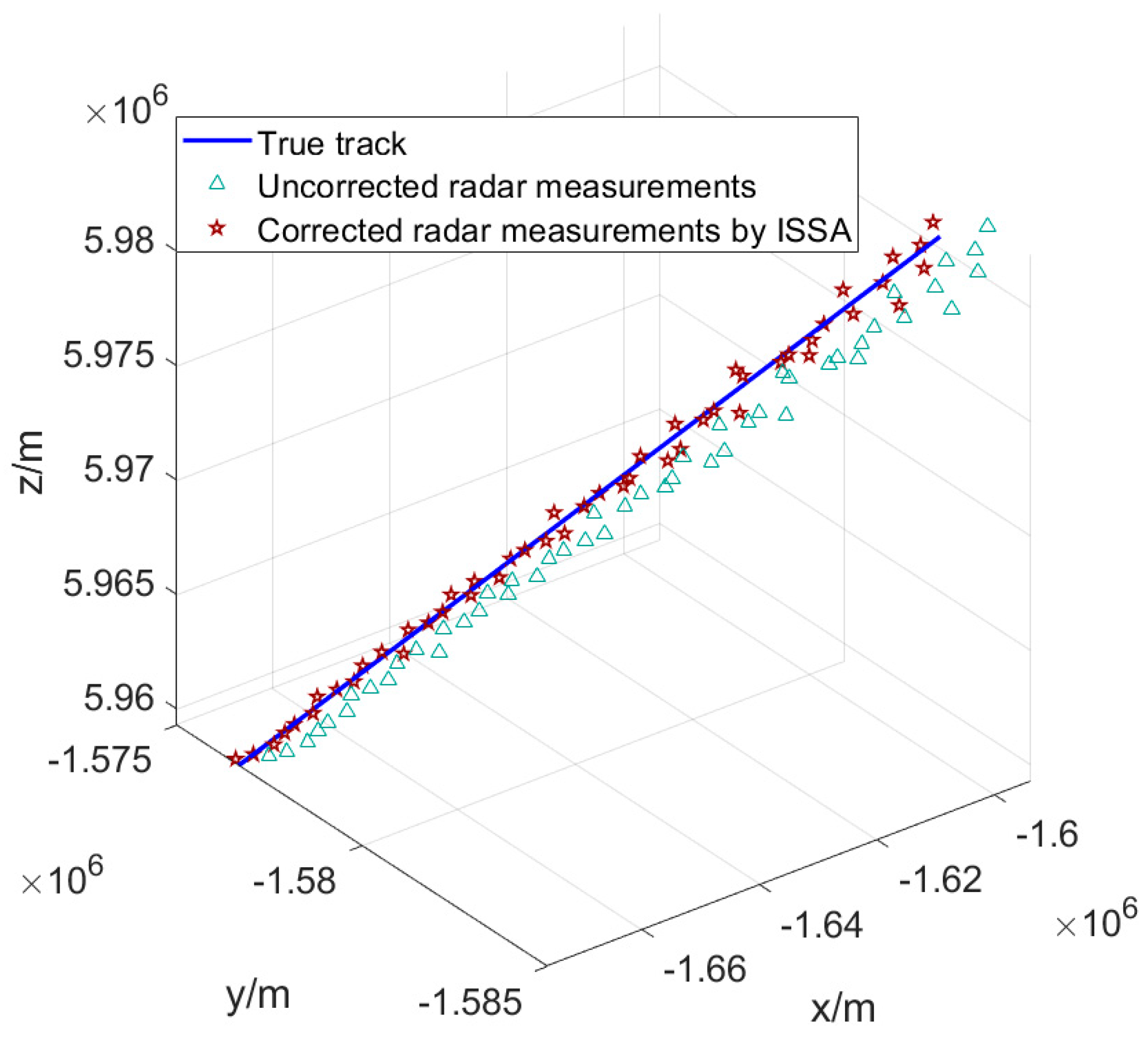
The estimated value of the systematic error was used to correct the radar observation results, and the target track comparison before and after correction was shown in Figure 5.
Obviously, the corrected radar measurement track is closer to the real track, but, due to the existence of measurement noise, there is still a certain difference between the radar observation track and the real track, which can be reduced through subsequent data processing (filtering, etc.).
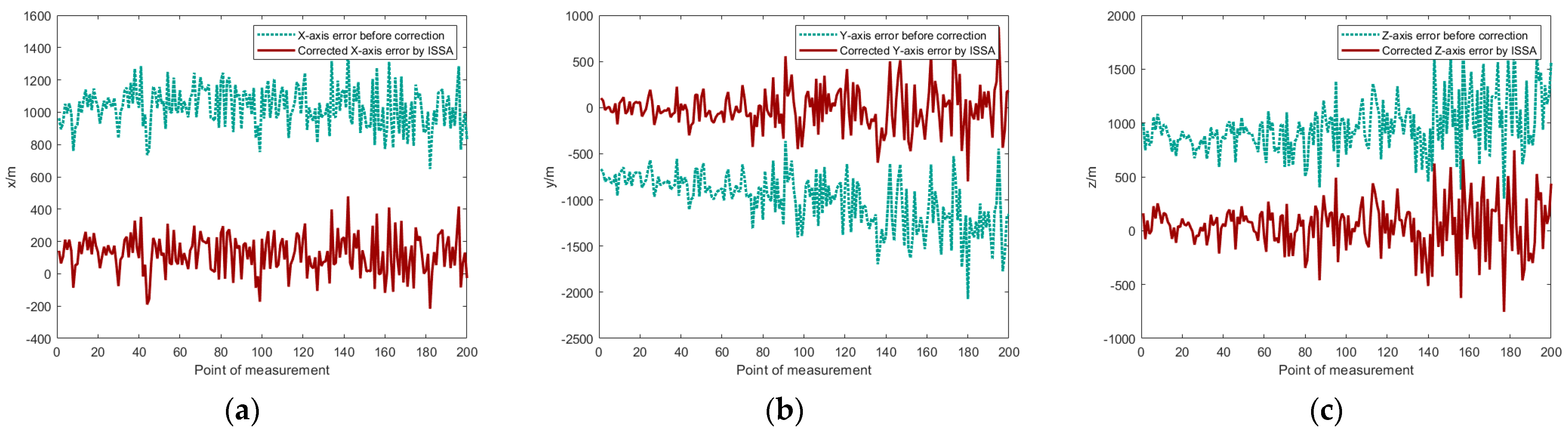
Figure 6 compares the radar observation errors before and after correction in the xyz triaxial direction. Here, 200 radar measurement values are taken along the triaxial direction, and the RMSE before and after correction is calculated as follows: the x-axis direction decreases from 1037.1 m before correction to 172.2 m after correction. The y-axis direction decreased from 1044.4 m before correction to 235.2 m; the z-axis direction decreased from 995.1 m to 222.5 m. It can be further calculated that the measurement accuracy of the corrected radar along the xyz axis is improved by 83%, 77%, and 78%, respectively. The above results show that the proposed method can significantly reduce the influence of systematic errors on the track of the target observed by the radar, and verify the effectiveness of the proposed method. Figure 6a shows that there is still a small amount of systematic error in the x-axis direction, which is because the algorithm’s estimation of the GNSS communication delay is not accurate enough. In addition, it can be seen from Figure 6b,c that, with the increase in measurement points, the error value fluctuates greatly, which is caused by the presence of azimuth measurement noise and elevation measurement noise. It also indicates the necessity of regular systematic error corrections in the radar system.
5. Conclusions
In this paper, a radar systematic error correction method based on cooperative targets is studied, and the measurement error model of the radar is established. In order to solve the problem of low accuracy of the radar systematic error estimation, an improved sparrow search algorithm is proposed to solve the systematic error, so as to avoid the accuracy loss caused by the linearization of nonlinear equations. At the same time, a variety of strategies are used to improve the sparrow search algorithm, which greatly improves the convergence speed, real-time performance, and stability of the algorithm, while taking into account the solving accuracy. The simulation results show that the method can significantly reduce the influence of systematic error on the radar measurement, and the target track accuracy is improved by 83%, 77%, and 78% in the triaxial directions, which verifies the effectiveness of the proposed method.
The method proposed in this paper is based on the assumption that the detection accuracy of different targets is consistent with that of the same radar system, but, in fact, the radar system displays slightly different processing of detection echoes of different targets. Some characteristics of targets (such as extremely strong radar cross-sectional area changes, special scattering characteristics, etc.) often require unconventional processing through the radar system, thus introducing additional errors, which then causes the radar to detect different targets with inconsistent accuracy. In the future, this error should be analyzed to improve the radar measurement error model, and a more universal error correction method should be studied.
Author Contributions
Conceptualization, Y.L. and B.F.; methodology, Y.L.; software, Y.L.; validation, Y.L., Z.S. and H.X.; formal analysis, Y.L.; investigation, Y.L.; resources, Z.S.; data curation, B.F.; writing—original draft preparation, Y.L.; writing—review and editing, Z.S.; visualization, H.X.; supervision, Z.S.; project administration, B.F. All authors have read and agreed to the published version of the manuscript.
Funding
This research received no external funding.
Institutional Review Board Statement
Not applicable.
Informed Consent Statement
Not applicable.
Data Availability Statement
The data presented in this study are available upon request from the corresponding author.
Acknowledgments
The authors would like to thank all the reviewers for their constructive comments. The program for the simulation of the proposed algorithm in this article was written with the MATLAB 2021b produced by Math-Works, Inc.
Conflicts of Interest
The authors declare no conflicts of interest.
References
- Yan, Y. Noise Suppression and Weak Signal Detection in Sea Clutter. Ph.D. Thesis, Nanjing University of Information Science and Technology, Nanjing, China, 2023; pp. 1–2. [Google Scholar]
- Wen, D.; Yi, H.; Zhang, W.; Xu, H. 2D-Unitary ESPRIT Based Multi-Target Joint Range and Velocity Estimation Algorithm for FMCW Radar. Appl. Sci. 2023, 13, 10448. [Google Scholar] [CrossRef]
- Ishtiaq, S.; Wang, X.; Hassan, S.; Mohammad, A.; Alahmadi, A.A.; Ullah, N. Three-Dimensional Multi-Target Tracking Using Dual-Orthogonal Baseline Interferometric Radar. Sensors 2022, 22, 7549. [Google Scholar] [CrossRef] [PubMed]
- Li, Z.; Cheng, T.; Heng, S. Real-time dwell scheduling algorithm for phased array radar based on a backtracking strategy. IET Radar Sonar Navig. 2022, 17, 261–276. [Google Scholar] [CrossRef]
- Liu, H.; Pu, Y.; Wang, H.; Chen, S.; Huang, Y. A data-driven systematic error estimation method for radar systems. J. Command. Control 2021, 7, 107–112. [Google Scholar]
- You, H.; Jianjuan, X.; Xin, G. Radar Data Processing with Applications; Publishing House of Electronics Industry: Beijing, China, 2022. [Google Scholar]
- Dong, Y.; Zhang, Y. A Review of Radar System Deviation Accurate Registration Technology[J/OL]. Modern Radar. Available online: https://kns.cnki.net/kcms/detail/32.1353.TN.20220905.1215.002.html (accessed on 5 September 2022).
- Jiang, B.; Sun, L.; Zhou, W.; Wang, G.; Guan, J. Multi-target joint Error Estimation method for sea-facing radar based on AIS. Fire Control Command. Control 2017, 9, 25–29. [Google Scholar]
- Ren, W.; Zhou, Z.; Lü, S.; Shi, D. Position calibration technique of ship based on information of AIS. Syst. Eng. Electron. 2016, 38, 2381–2388. [Google Scholar]
- Li, S.; Su, Y. Registration for Multi-Sensor Networking System. Mod. Navig. 2021, 12, 438–443. [Google Scholar]
- Shang, J.; Yao, Y. Approach of system error registration for two-station coast radars for sea surface monitoring. J. Eng. 2019, 21, 7721–7725. [Google Scholar] [CrossRef]
- Chang, C.; Zhao, Q.; Yu, H.; Shen, L.; Dong, H. Approach for Space Registration Based on Extreme Learning Machines. Fire Control Command. Control 2017, 42, 10–13. [Google Scholar]
- Luo, J.; Shang, Y.; Zeng, H.; Wang, Y. Coast Radar Calibration Method Based on Automatic Identification System (AIS) Information. Telecommun. Eng. 2009, 49, 87–89. [Google Scholar]
- Pan, S.; Cha, H. A study on shipborne radar calibration method based on AIS. Ship Sci. Technol. 2009, 31, 101–104+127. [Google Scholar]
- Dong, Y.; Huang, G.; Li, B.; Zhang, L.; Guan, J. Error Analysis of Sea Radar System Based on AIS Auxiliary Information. Mod. Radar 2020, 42, 17–23. [Google Scholar]
- Zhang, Y.; Wang, G.H.; Chen, L. Real-Time Robust Estimation of Sensor Bias for Radar Network under Multi-Target Circumstance. Electron. Opt. Control 2013, 20, 5–7+27. [Google Scholar]
- Yuan, C. Research on Radar System Error Registration Technology Based on ADS-B. Master’s Thesis, Southern Medical University, Guangzhou, China, 2020. [Google Scholar]
- Ding, L.; Geng, F.; Chen, J. Radar Principle; Publishing House of Electronics Industry: Beijing, China, 2020; pp. 206–210. [Google Scholar]
- Dong, Y.; Huang, G.; Li, B.; Liu, N.; Chen, X. High precision error calibration method for radar based on AIS. Appl. Electron. Tech. 2019, 45, 75–79. [Google Scholar]
- Dong, Y.; Huang, G.; Li, B. A Calibration Method Based on Radar Coverage Partitioning Under Non-uniform System Errors. Electron. Opt. Control 2020, 27, 69–74. [Google Scholar]
- Wu, Z.Y.; Wang, M.H.; Zhang, R.P. ADS-B-Based Algorithm for Real-Time Optimal Estimation of Radar Biases. J. Southwest Jiaotong Univ. 2013, 48, 102–106+115. [Google Scholar]
- You, H.; Zhu, H.; Tang, X. Joint systematic error estimation algorithm for radar and automatic dependent surveillance broadcasting. IET Radar Sonar Navig. 2013, 7, 361–370. [Google Scholar] [CrossRef]
- Li, P.; Fan, E.; Yuan, C. A Specific Iterative Closest Point Algorithm for Estimating Radar System Errors. IEEE Access 2020, 8, 6417–6428. [Google Scholar] [CrossRef]
- Zhang, T.; Wu, R.; Lai, R.; Zhang, Z. Probability hypothesis density filter for radar systematic bias estimation aided by ADS-B. Signal Process. 2016, 120, 280–287. [Google Scholar] [CrossRef]
- Cheng, L.; Zhang, H.; Wei, D.; Zhou, J. An Indoor Tracking Algorithm Based on Particle Filter and Nearest Neighbor Data Fusion for Wireless Sensor Networks. Remote Sens. 2022, 14, 5791. [Google Scholar] [CrossRef]
- Lyu, X.Y.; Wang, J. Sequential Multi-sensor JPDA for Target Tracking in Passive Multi-static Radar with Range and Doppler Measurements. IEEE Access 2019, 7, 34488–34498. [Google Scholar] [CrossRef]
- Guo, S.; Mou, J.; Chen, L.; Chen, P. Improved kinematic interpolation for AIS trajectory reconstruction. Ocean. Eng. 2021, 234, 109256. [Google Scholar] [CrossRef]
- Zhu, T.; Chang, G.; Chen, C.; Zhang, L.; Zhang, S. Continuous modelling of global navigation satellite system multipath errors for sidereal filtering. IET Radar Sonar Navig. 2020, 14, 303–312. [Google Scholar] [CrossRef]
- Luo, T.; Xie, J.; Zhang, B.; Zhang, Y.; Li, C.; Zhou, J. An improved levy chaotic particle swarm optimization algorithm for energy-efficient cluster routing scheme in industrial wireless sensor networks. Expert Syst. Appl. 2024, 28, 122780. [Google Scholar] [CrossRef]
- Lei, M.; Wu, B.; Li, P.; Yang, W.; Xu, J.; Yang, Y. A fast convergence strategy based on gray wolf optimization algorithm for co-estimation of battery state of charge and capacity. Electrochim. Acta 2024, 474, 143525. [Google Scholar] [CrossRef]
- Yue, Y.; Cao, L.; Lu, D.; Hu, Z.; Xu, M.; Wang, S.; Li, B.; Ding, H. Review and empirical analysis of sparrow search algorithm. Artif. Intell. Rev. 2023, 56, 10867–10919. [Google Scholar] [CrossRef]
- Xue, J.; Shen, B. A novel swarm intelligence optimization approach: Sparrow search algorithm. Syst. Sci. Control Eng. 2020, 8, 22–34. [Google Scholar] [CrossRef]
- Liu, G.; Wu, Q.; Wang, G.; Jin, P. A Improved Logistic Chaotic Map and Its Application to Image Encryption and Hiding. J. Electron. Inf. Technol. 2022, 44, 3602–3609. [Google Scholar]
- Chen, L.; Song, N.; Ma, Y. Harris hawks optimization based on global cross-variation and tent mapping. J. Supercomput. 2022, 79, 31–39. [Google Scholar] [CrossRef]
- Feng, J.; Zhang, J.; Zhu, X.; Lian, W. A novel chaos optimization algorithm. Multimed. Tools Appl. 2017, 76, 17405–17436. [Google Scholar] [CrossRef]
- Liu, X. Research on Deployment Algorithm of Underwater Sensor Network. Master’s Thesis, Jilin University, Changchun, China, 2023. [Google Scholar]
- Wu, D.; Rao, H.; Wen, C.; Jia, H.; Liu, Q.; Abualigah, L. Modified Sand Cat Swarm Optimization Algorithm for Solving Constrained Engineering Optimization Problems. Mathematics 2022, 10, 4350. [Google Scholar] [CrossRef]
- Dehghani, M.; Trojovský, P. Osprey optimization algorithm: A new bio-inspired metaheuristic algorithm for solving engineering optimization problems. Front. Mech. Eng. 2023, 8, 1126450. [Google Scholar] [CrossRef]
- Yang, X.; Liu, J.; Liu, Y.; Xu, P.; Yu, L.; Zhu, L.; Chen, H.; Deng, W. A Novel Adaptive Sparrow Search Algorithm Based on Chaotic Mapping and T-Distribution Mutation. Appl. Sci. 2021, 11, 11192. [Google Scholar] [CrossRef]
- Zhang, W.; Liu, S. Improved sparrow search algorithm based on adaptive t-distribution and golden sine and its application. Microelectron. Comput. 2022, 39, 17–24. [Google Scholar]
- Li, J.; Zhao, C.; Chen, J.; Zhao, R. A Modified Generalized Least Square Registration Algorithm on WGS-84 Coordinate. J. Shanghai Jiaotong Univ. 2016, 50, 771–775. [Google Scholar]
Figure 1.
Radar measurement error.
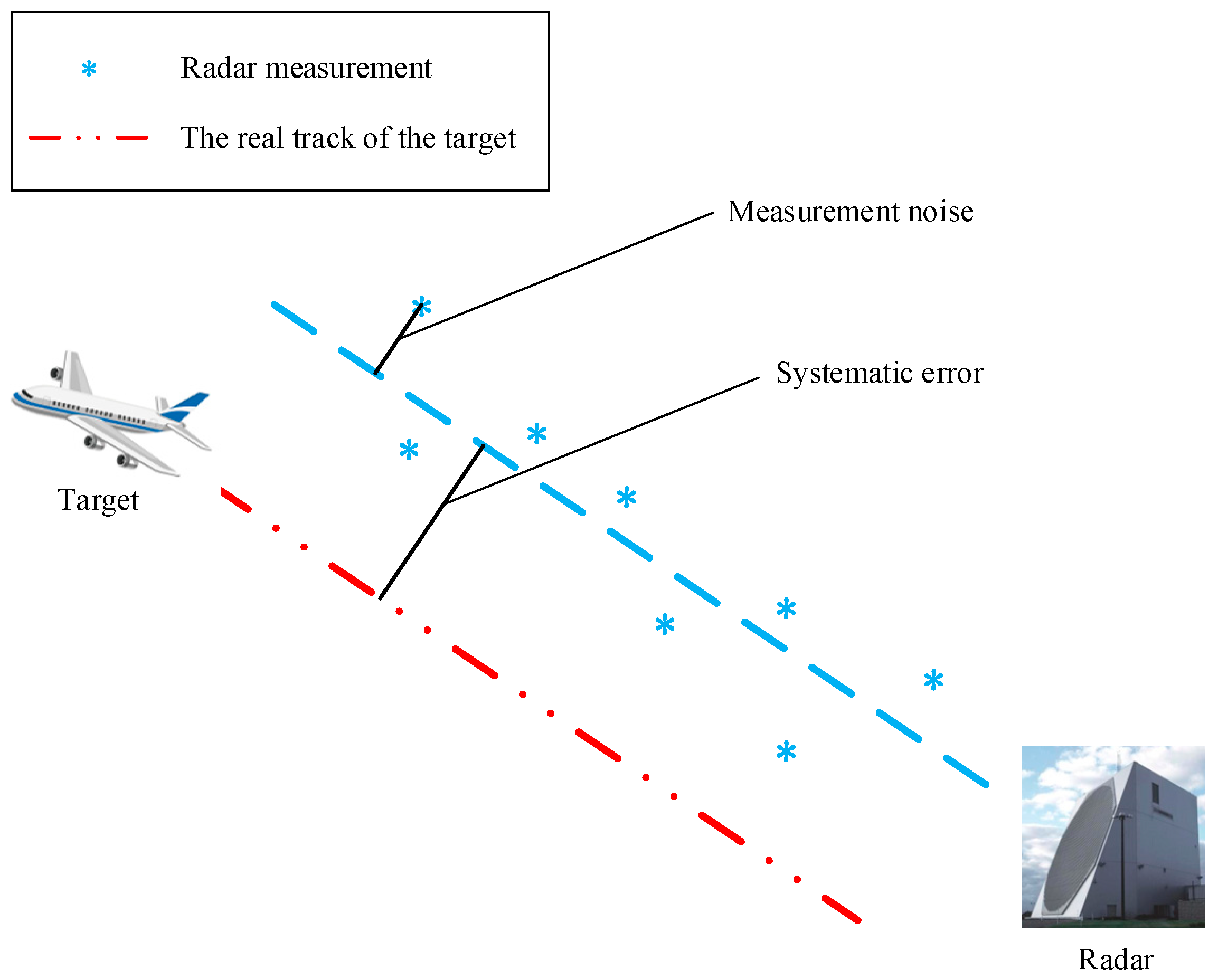
Figure 2.
Calibration principle of the radar system based on the cooperative target.
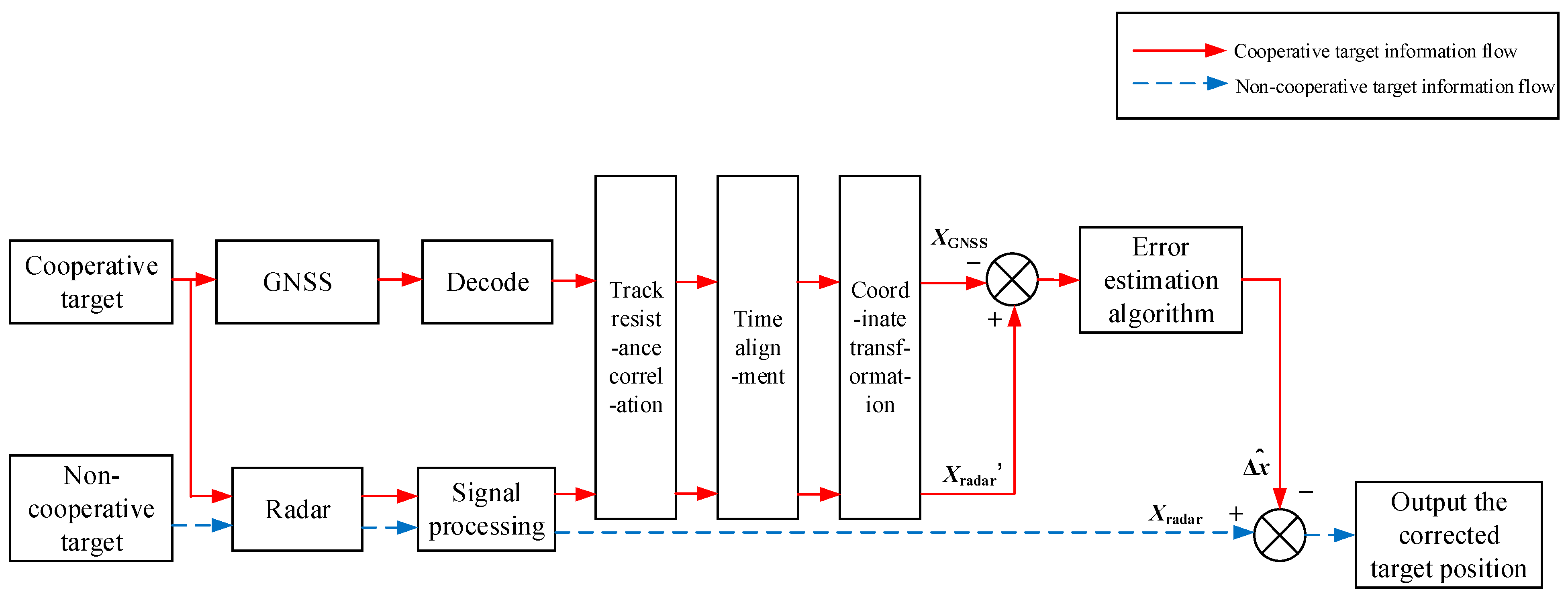
Figure 3.
ISSA flowchart.
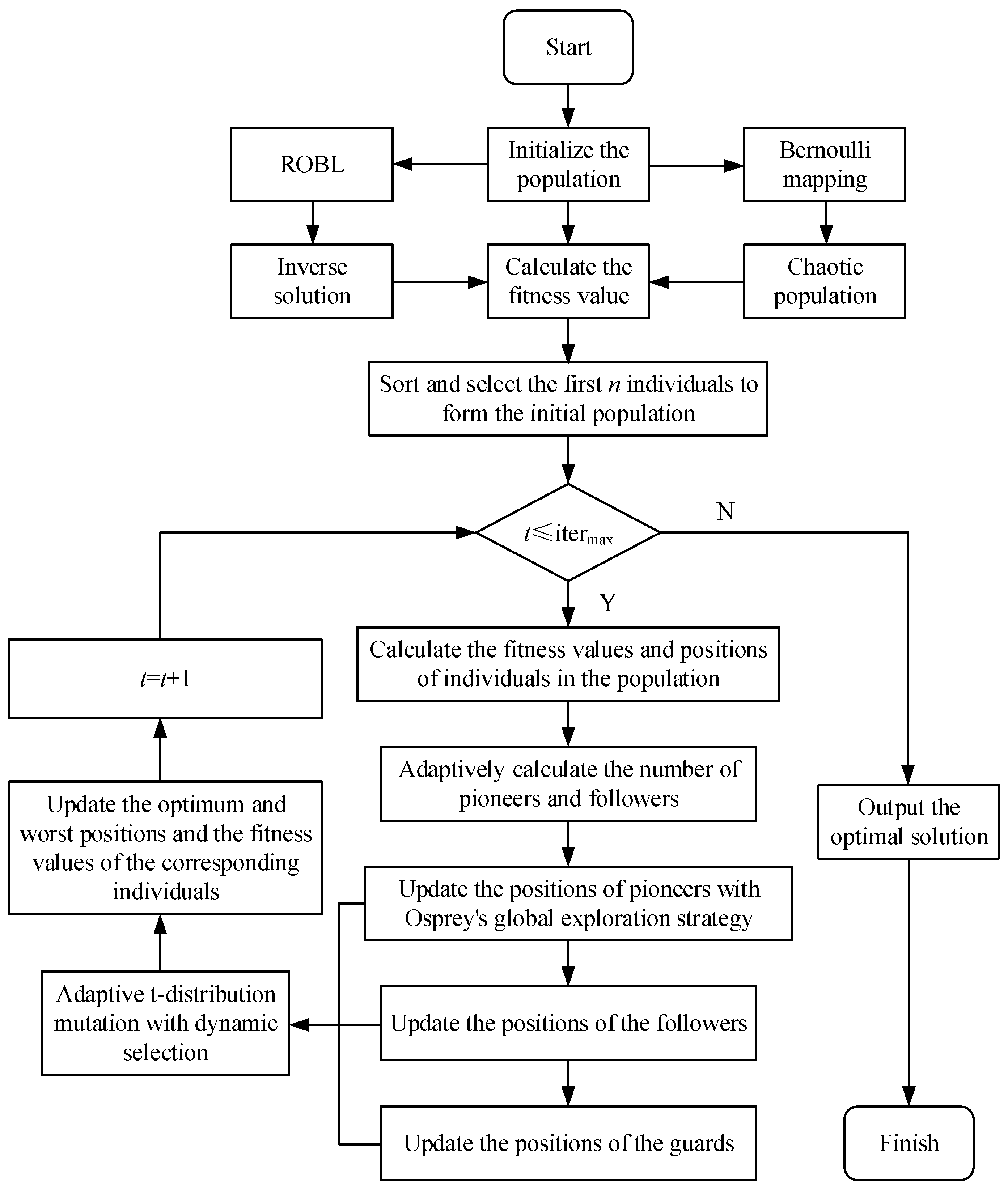
Figure 4.
The RMSE of the radar systematic error estimation under different measurement points. (a) Range systematic error; (b) Azimuth systematic error; (c) Elevation systematic error; (d) Communication delay.
Figure 4.
The RMSE of the radar systematic error estimation under different measurement points. (a) Range systematic error; (b) Azimuth systematic error; (c) Elevation systematic error; (d) Communication delay.
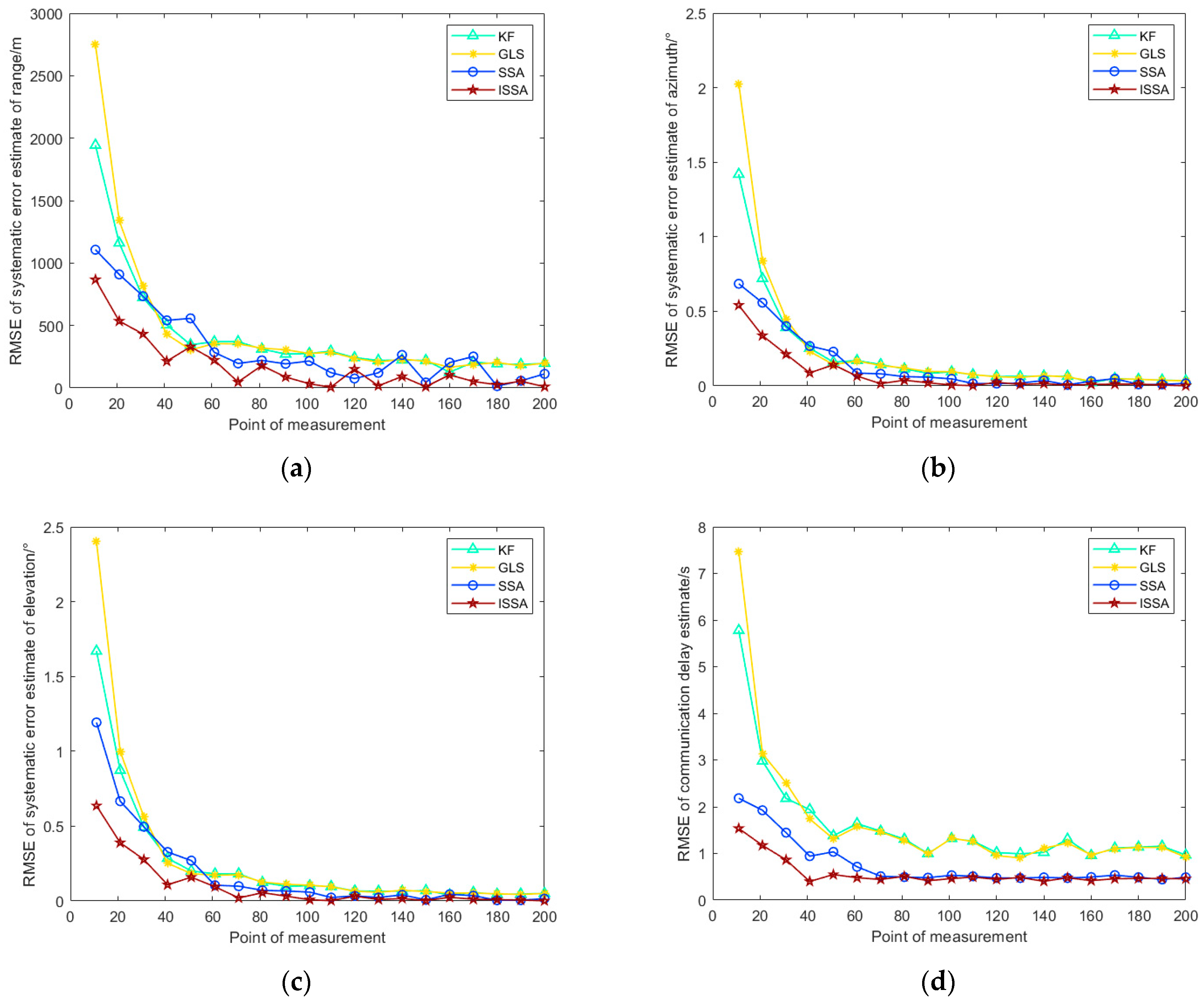
Figure 5.
Target real track and radar measurement comparisons before and after calibration.

Figure 6.
Error correction effect. (a) x-axis error; (b) y-axis error; (c) z-axis error.

Table 1.
Simulation conditions.
| Simulation Parameter | Symbol | Value |
|---|---|---|
| Radar geographic coordinates | (68.923°, −137.259°, 51.856 m) | |
| Range systematic error | 1300 m | |
| Azimuth systematic error | 0.498° | |
| Elevation systematic error | 0.544° | |
| Communication delay | 1 s | |
| Measurement noise of range | 80 m | |
| Measurement noise of azimuth | 0.2° | |
| Measurement noise of elevation | 0.2° |
Table 2.
Performance comparison of different algorithms.
| Evaluation Index | Error Estimation Algorithm | ||||
|---|---|---|---|---|---|
| KF | GLS | SSA | ISSA | ||
| (m) | RMSE | 204.49 | 198.62 | 148.11 | 77.44 |
| (°) | RMSE | 0.0364 | 0.0352 | 0.0216 | 0.0075 |
| (°) | RMSE | 0.0463 | 0.0450 | 0.0243 | 0.0098 |
| (s) | RMSE | 0.9195 | 0.8973 | 0.4844 | 0.4667 |
| Average time consuming(s) | 0.0072 | 0.0111 | 0.8206 | 0.4687 | |
Disclaimer/Publisher’s Note: The statements, opinions and data contained in all publications are solely those of the individual author(s) and contributor(s) and not of MDPI and/or the editor(s). MDPI and/or the editor(s) disclaim responsibility for any injury to people or property resulting from any ideas, methods, instructions or products referred to in the content. |
© 2024 by the authors. Licensee MDPI, Basel, Switzerland. This article is an open access article distributed under the terms and conditions of the Creative Commons Attribution (CC BY) license (https://creativecommons.org/licenses/by/4.0/).
Share and Cite
MDPI and ACS Style
Liu, Y.; Shi, Z.; Fu, B.; Xu, H. Radar Error Correction Method Based on Improved Sparrow Search Algorithm. Appl. Sci. 2024, 14, 3714. https://doi.org/10.3390/app14093714
AMA Style
Liu Y, Shi Z, Fu B, Xu H. Radar Error Correction Method Based on Improved Sparrow Search Algorithm. Applied Sciences. 2024; 14(9):3714. https://doi.org/10.3390/app14093714
Chicago/Turabian StyleLiu, Yifei, Zhangsong Shi, Bing Fu, and Huihui Xu. 2024. "Radar Error Correction Method Based on Improved Sparrow Search Algorithm" Applied Sciences 14, no. 9: 3714. https://doi.org/10.3390/app14093714
Note that from the first issue of 2016, this journal uses article numbers instead of page numbers. See further details here.