
Gas–Liquid Two-Phase Flow Measurement Based on Optical Flow Method with Machine Learning Optimization Model
Department of Instrumentation Engineering, College of Metrology and Measurement Engineering, China Jiliang University, Hangzhou 310018, China
*
Author to whom correspondence should be addressed.
Appl. Sci. 2024, 14(9), 3717; https://doi.org/10.3390/app14093717
Submission received: 15 March 2024
/
Revised: 24 April 2024
/
Accepted: 25 April 2024
/
Published: 26 April 2024
(This article belongs to the Special Issue Advanced Heat and Mass Transfer Techniques in Power and Energy Systems)
Abstract
:Featured Application
Application to the monitoring of gas–liquid two-phase flow links.
Abstract
Gas–Liquid two-phase flows are a common flow in industrial production processes. Since these flows inherently consist of discrete phases, it is challenging to accurately measure the flow parameters. In this context, a novel approach is proposed that combines the pyramidal Lucas-Kanade (L–K) optical flow method with the Split Comparison (SC) model measurement method. In the proposed approach, videos of gas–liquid two-phase flows are captured using a camera, and optical flow data are acquired from the flow videos using the pyramid L–K optical flow detection method. To address the issue of data clutter in optical flow extraction, a dynamic median value screening method is introduced to optimize the corner point for optical flow calculations. Machine learning algorithms are employed for the prediction model, yielding high flow prediction accuracy in experimental tests. Results demonstrate that the gradient boosted regression (GBR) model is the most effective among the five preset models, and the optimized SC model significantly improves measurement accuracy compared to the GBR model, achieving an R2 value of 0.97, RMSE of 0.74 m3/h, MAE of 0.52 m3/h, and MAPE of 8.0%. This method offers a new approach for monitoring flows in industrial production processes such as oil and gas.
1. Introduction
Gas–liquid two-phase flow is a common flow across various industries, including petroleum, chemical, natural gas, thermal power generation, aerospace, and nuclear energy. Accurately measuring parameters in such flows is crucial for the efficient and stable operation of industrial systems and production activities. However, due to the complexity of affecting factors like flow structure, physical characteristics, flow rate, pressure, heat treatment, pipeline, and geometry, it is an enormous challenge to perform accurate measurements using traditional methods [1]. Currently, the measurement of gas–liquid two-phase flow rates in gas, oil, and chemical processes often involves the use of separation methods, which require a large space and expensive equipment [2]. While this challenge can be effectively resolved using non-separation measurement methods, they have limitations in terms of measurement range and medium. For instance, the performance of Doppler technology-based methods is affected by flow patterns, which may adversely affect the measurement accuracy. Additionally, there are significant differences in physical properties such as density and sound speed between gases and liquids, which may affect ultrasound propagation and measurement accuracy [3]. Therefore, it is of significant importance to develop a low-cost, accurate, and convenient method for measuring gas–liquid two-phase flow rates. Studies show that intelligent learning algorithms have significant advantages in addressing nonlinear and multivariate problems and can effectively improve the applicability of non-separation measurement methods. Consequently, exploring the application of intelligent learning algorithms in measuring gas–liquid two-phase flow rates has become a hot research topic in recent years. In this context, Zhiyue Zhao et al. [4] utilized acoustic emission (AE) and near-infrared (NIR) sensors to capture resonance peak edge factors, and subsequently employed the least absolute shrinkage selection operator (LASSO) machine learning technique to predict gas–liquid two-phase void fraction and flow rate. This approach achieved an 89.47% accuracy within a 20% relative error margin for emulsion flow data. Shanshan Li et al. [5] proposed a physics-guided deep learning model by integrating a physical constraint term of the rates of change of pressure caused by the slip term to maintain consistency in the gas and liquid phases into the loss function of a deep neural network. This physics-guided neural network (PGNN) successfully measured gas and liquid flow rates simultaneously with a high accuracy, even under a wide range of test conditions (gas volume fraction (GVF) > 95%). Furthermore, Shanshan Li et al. [6] predicted gas and liquid flow rates in intermittent flows using information from a cone gauge and a conductivity loop sensor. The predicted liquid mass flow rate had a relative error of less than ±5.0% at a 99% confidence level, while for the gas phase, the relative error was within ±15.0% at a 98% confidence level. Delin Hu et al. [7] applied convolutional neural networks (CNNs) to multiphase flow rate prediction, introducing the flow adversarial network (FAN). Experimental results demonstrated a mean absolute percentage error (MAPE) of up to 8.36% and 9.09%. Zhongke Gao et al. [8,9] developed a multi-task-based time-channel convolutional neural network (MTCCNN) to predict porosity, achieving a superior performance in gas phase gas content prediction. Additionally, they designed a segmented dense connectivity network (SDCN), capable of simultaneously measuring the total rate and void ratio using signals from a four-sector conductivity sensor. The framework exhibited a high accuracy in the total flow measurement of gas–liquid two-phase flow within a range of 0.18–1.23 m3/h.
Integrating sensors with intelligent learning models is a complex process with high measurement requirements and associated costs. Sensor-based approaches can be cumbersome, requiring intricate installation and maintenance, especially as the flow condition becomes more chaotic, leading to noticeable signal interference. Alternatively, employing image processing techniques can greatly improve the convenience of measurement methods. However, current applications primarily focus on two-phase flow pattern classification in research on gas–liquid two-phase flow pattern classifications in research on gas–liquid two-phase flow patterns within an S-shaped watertight pipe, achieving detection and validation accuracies of 98.13% and 98.06%, respectively. Jinsong Zhang et al. [10] utilized the GoogLeNet+5 algorithmic model for flow pattern recognition on image datasets of various liquid–liquid two-phase flows such as Nalgioil and GaInSn-Water, achieving training and testing accuracies of 95.09% and 98.12%, respectively. Feng Nie et al. [11] utilized CNN algorithms to classify flow patterns in images of methane and tetrafluoromethane within horizontal circular pipes, achieving a testing dataset accuracy exceeding 90.63% and an average accuracy surpassing 97.56% for all data points in the database. Zhongke Gao et al. [12] designed a branch-aggregation network (BAN) for classifying flow patterns in gas–liquid two-phase flow images, achieving a fast convergence speed and a recognition accuracy of 99.60%, highlighting its advantage in noise resistance. Zhong-Ke Gao et al. [13] proposed a deep learning method based on complex networks that combined the original signals of limited penetrable visibility graphs (LPVG) with images for flow pattern classification and gas void fraction measurement. Their results showed a classification accuracy of 95.3% and an average root mean square error (RMSE) of 0.0038, with an average absolute percentage error of 6.3% for gas void fraction measurement. Shai Kadish et al. [14] utilized computer vision techniques and deep learning to train CNNs and long short-term memory (LSTM) networks for classifying fluid flow states using video frames as features. They also measured steam mass flow rates within the range of (0.005 to 0.023) kg/s, with an average RMSE of 5% of full scale, achieving a classification accuracy of 92%.
There are also notable research outcomes in gas–liquid two-phase flow pattern classifications utilizing non-image processing methods combined with intelligent learning models. Boyu Kuang et al. [15] employed ultrasonic sensors and a convolutional recurrent neural network (CRNN) to identify gas–liquid two-phase flow patterns within an S-shaped watertight pipe, achieving detection and validation accuracies of 98.13% and 98.06%, respectively. Lei OuYang et al. [16] proposed a deep neural network framework to utilize acquired signals. By employing two slicing operations combined with a bidirectional long-short memory network (BiLSTM) and a CNN, they attained an average recognition accuracy of 99.32%. Zhiee Jhia Ooi et al. [17] utilized conductivity probe signals as input data to identify the flow state of boiling flow in vertical annular channels and proposed a two-step method using unsupervised self-organizing map (SOM) to recognize local and global flow states, achieving a classification accuracy of over 90%. Somtochukwu Godfrey Nnabuife et al. [18] introduced a method for classifying flow states using deep neural networks (DNNs), which operate on features extracted from Doppler ultrasound signals using fast Fourier transform (FFT). Experimental results demonstrated that DNNs achieved a classification accuracy of 99.01%. Additionally, Somtochukwu Godfrey Nnabuife et al. [19] proposed a new method for feature extraction from preprocessed data, named belt-shaped features (BSFs), which were applied to ConvNet classifiers, achieving accuracy rates of 97.40%, 94.57%, and 94.94% for the training set, test set, and validation set, respectively. Harold Brayan Arteaga-Arteaga et al. [20] selected 12 databases to train and test machine learning models, with experimental results showing that the extra trees model classified flow patterns with the highest fidelity, achieving an accuracy of 98.8%. Radosław Wajman et al. [21] utilized 3D electrical capacitance tomography (ECT) measurement data to establish and train artificial neural network models, with experimental results indicating that the fuzzy pattern recognition accuracy of the horizontal case ranged from 85% to 99%, and in the vertical case, the accuracy fluctuated from 65% to above, with the average correct recognition rate for fuzzy reasoning based on raw ECT data without images being approximately 90%. Lifeng Zhang et al. [22] proposed a method for identifying flow patterns based on Gramian angular field (GAF) and densely connected network (DenseNet), with experimental results demonstrating that GAF images effectively reflected the characteristics of different flow patterns, achieving an average flow pattern recognition accuracy of 98.3%. Haobin Chen et al. [23] introduced an intrusive robust CNN flow pattern recognition method, based on flow-induced vibration (FIV) analysis, with the accuracy rate being above 90% when using different axis data to predict flow patterns. Noor Hafsa et al. [24] compared and analyzed machine learning (ML) and deep learning (DL), concluding that extreme gradient boosting is the optimal model for predicting the two-phase flow states of inclined or horizontal pipelines.
In conclusion, the application of intelligent learning algorithms in classifying flow patterns of gas–liquid two-phase flow has reached a notable level of accuracy, and promising advancements have also been made in flow measurement. However, current methods for combining sensors with intelligent learning models for measurement pose challenges in installation and susceptibility to signal disturbances. Similarly, the integration of images with intelligent learning models faces hurdles in achieving precise measurements solely based on a single image due to the intricate nature of the gas–liquid two-phase flow. Therefore, it is crucial to explore the feasibility of combining video with intelligent learning models for flow measurements, aiming to achieve convenient flow rate measurements through camera-based approaches.
This article delves into a novel approach for flow measurements using gas–liquid two-phase flow videos, focusing on extracting pertinent information from the video via optical flow methods. It investigates the integration of this extracted data with machine learning models, aiming to enhance measurement accuracy. Through an exploration of diverse machine learning models, this study identifies and optimizes the most effective model, thereby improving measurement outcomes. This method facilitates more convenient and real-time measurements of two-phase flows, offering a fresh avenue for daily monitoring of two-phase flow rates in the oil and natural gas industry through camera-based acquisition.
2. Materials and Methods
2.1. Gas–liquid Two-Phase Flow Experimental Setup and Data Acquisition
The gas–liquid two-phase flow video is captured using the device shown in Figure 1. The device primarily consists of a water pump, air pump, pressure stabilizer tube, flow stabilizer tank, valve, liquid flow meter, gas flow meter, and water tank.
During the experiment, a cell phone was positioned parallel to the vertical transparent tube section at a distance ranging from 10 to 20 cm for video capture. The diameter of the tube section was 25 mm, and the height of the observation point from the entrance of the vertical tube was 1 m, ensuring that the gas–liquid two-phase flow reached a fully developed state. The video recording equipment settings were 1920 × 1080 pixels resolution at 60 frames per second (fps). The experimental flow range was between 1 and 16 m3/h. Based on G.F. Hewitt’s classification [25] of gas–liquid two-phase flow patterns in vertically ascending adiabatic tubes, the flow patterns were classified as annular, churn, bubbly, and slug flow shown in Figure 2.
The dataset comprised 33 video clips depicting annular flow, 26 clips showing churn flow, 79 clips displaying bubbly flow, and 48 clips illustrating slug flow.
The experimental data were extracted from videos of adequate length, reflecting the flow characteristics. The videos were segmented into 1 s clips with a resolution of 1920*1080 pixels and a frequency of 60 fps. A dataset comprising 186 video clips was utilized for feature extraction, model training, and testing of the two-phase flow. Of these, 80% of the data were randomly selected for the training set, while the remaining 20% were allocated to the test set to evaluate the regression model. The total flow distribution is illustrated in Figure 3.
2.2. Optical Flow Detection and Regression Modeling
This section outlines the process of optical flow extraction for gas–liquid two-phase flow videos, detailing optical flow data fusion, feature engineering, and model selection [26].
2.2.1. Pyramid L–K Optical Flow Feature Extraction
The optical flow method enables the observation of pixel point motion within spatial objects depicted in an image, offering insights into the movement of bubbles within gas–liquid two-phase flow videos. Predicated on the assumption of constant brightness, the method interprets motion as “small motion” along the time continuum. This realization is based on the fundamental constraint equations affirming constant light intensity at characteristic pixel points before and after motion, as expressed in Equation (1) [27].
where I is the grayscale value of a pixel point in the image, x represents the horizontal coordinate of the pixel point in the image, y represents the vertical coordinate of the pixel point in the image, and t represents time, s.
With , the Taylor expansion of Equation (1) can be expressed in the form below:
where u and v are the optical flow vectors used to calculate the motion of bubbles in the image.
In this study, the pyramid Lucas–Kanade (L–K) optical flow method is selected to capture the sparse optical flow. This method has been commonly applied for analysis and recording without computing every pixel in the video, focusing solely on the bubble features within the pipeline. The pyramid optical flow method addresses the challenge of high-speed motion in video frames when the flow rate is large, while the L–K optical flow method is more suitable for fitting the optical flow at lower speeds [28,29].
The corner function, which is used to identify the feature points or corners within an image, is crucial for computing the sparse optical flow. These feature points are typically chosen at corner locations because they exhibit significant changes in pixel brightness when a small window is shifted by a distance (dx, dy). This characteristic aligns well with the requirements of Lucas–Kanade optical flow calculation, particularly in scenarios involving bubble edges. Optical flow calculations entail measuring the displacement of these corner points between the two consecutive frames. The corner function can be mathematically defined as follows:
where E(dx, dy) represents the grayscale change in the window after movement, w(x, y) is a window weight function, and I(x + dx, y + dy) – I(x, y) calculates the grayscale change in the window after movement.
In the experiment, the Harris feature detection algorithm was employed to identify the corner points within the video frames of the two-phase flow. Subsequently, through robust feature tracking, the displacement of these corner points between adjacent frames was calculated using the pyramid Lucas–Kanade (L–K) optical flow method [30].
Harris corner detection incorporates the concept of Harris response R, which avoids the need to solve for eigenvectors, making the computation process more efficient [31]:
where R is Harris response value, k is a parameter ranging from 0.04 to 0, , , and .
The pyramid optical flow computation involves adjusting the size of the detected image by creating an image “pyramid,” with the original image serving as layer 0. The image is then reduced by a factor of 2 L to create multiple layers, where L represents the number of pyramid levels. The top layer corresponds to the image with the lowest resolution, while the bottom layer retains the original image size. In the gas–liquid flow data acquisition setup, a 3-layer pyramid structure was employed, with the top layer (L = 3) having an image size of 240 × 135 pixels, derived from the original image size of 1920 × 1080 p. Optical flow calculations were conducted using the top-layer image, and the results were then enlarged by a factor of two to use as initial optical flow estimates for calculations in the lower layers.
where L is the pyramid layer number, g is the initial optical flow estimate, and d is the calculated optical flow.
The optical flow of the original image is obtained through iteration, during which the sum of pixel-matching errors within the window used is calculated and minimized to compute the optical flow. This process can be mathematically expressed as follows:
where is the grayscale change within the window, ux and uy represent the coordinates of the tracked point, wx and wy are the neighborhood window, and v is the optical flow.
The derivation of the above equation involves setting the derivative at the optimal solution to zero. This can be achieved by performing a first-order Taylor expansion and neglecting the high-order terms.
where , , and get:
where v is the optical flow.
In this process, the image J is shifted by the previously calculated optical flow v distance to form a new window. The optical flow is then iteratively computed. A threshold of 0.01 is set for iteration, and the maximum number of iterations is set to 150. The optical flow obtained after k iterations is denoted as .
where is the optical flow obtained from the kth iteration, is the optical flow obtained from the (k − 1)th iteration, is the optical flow obtained from the current calculation.
The data obtained from the optical flow acquisition of 187 gas–liquid two-phase flow videos using the pyramid L–K optical flow method were considerable. To simplify the calculations, one gas–liquid two-phase flow video was randomly selected for analysis in this section. The first 30 frames of this video were utilized for optical flow computation, and corner points exhibiting minimal movement were extracted with a threshold set to 100. Subsequently, a significant number of displacements of corner points from the optical flow were obtained from the experiment. For each corner point, the initial position obtained from the optical flow algorithm in this video was recorded, along with the position of optical flow computation, the displacement di, and the displacement components dix and diy in the x and y directions, respectively, were computed using the following equations:
where xi1 represents the position of the current i-th corner point in the previous frame; xi2 represents the position of the current i-th corner point in the next frame; dix represents the displacement of the current i-th corner point in the x-direction, measured in pixels; diy represents the displacement of the current i-th corner point in the y-direction, measured in pixels; di represents the magnitude of the optical flow for the current i-th corner point, measured in pixels.
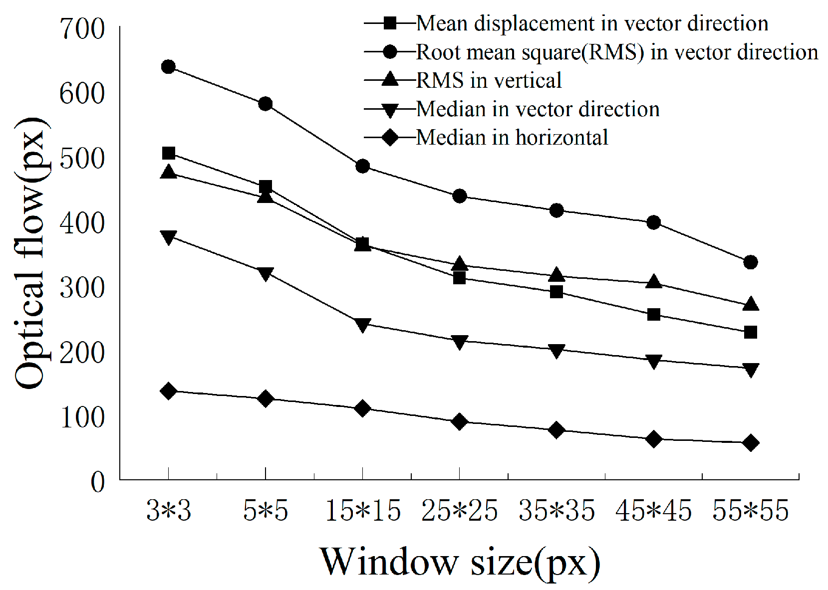
To provide a more intuitive representation of the data obtained from the optical flow acquisition method, the root-mean-square (RMS) value, median value, and average optical flow parameter of the corner point displacements are utilized as the reference parameters.
Figure 4 indicates that the average displacements of the corner points under various window sizes significantly exceed the median displacements in each direction. This observation demonstrates that a considerable portion of the corner point displacements are small in the optical flow calculations, resulting in low median values. Consequently, the corner point acquisition process incorporates more interfering corner points with smaller displacements, which may not correspond to the actual flow measurements. Given that the threshold value of 100 may not be universally applicable to all flow states, the implementation of a dynamic threshold corner screening method becomes necessary.
The flow state is annular and contains chaotic gas–liquid flow and bubbles. A larger window size is not conducive to the optical flow collection of small bubbles. Additionally, it may decrease the precision of the optical flow, resulting in larger errors in the calculations. Figure 5 depicts the current frame picture and the corner point collection.
Figure 5 illustrates the distribution of corner points for a frame in both annular and elastic flow videos, both of which were captured using a 55*55 px window. A constant-value corner sieving method was employed, resulting in fewer corners being captured for smaller flows. It is worth noting that capturing small bubbles in the elastic and annular flows is crucial in the gas–liquid optical flow acquisition process. The size of these small bubbles is approximately 1/24 of the height of the acquisition area, corresponding to a height of 45 pixels in an overall pixel height of 1080. Considering the relative height of the top image after pyramid transformation, which is approximately 6 px, a 5*5 px window was chosen for optical flow calculation in this study.
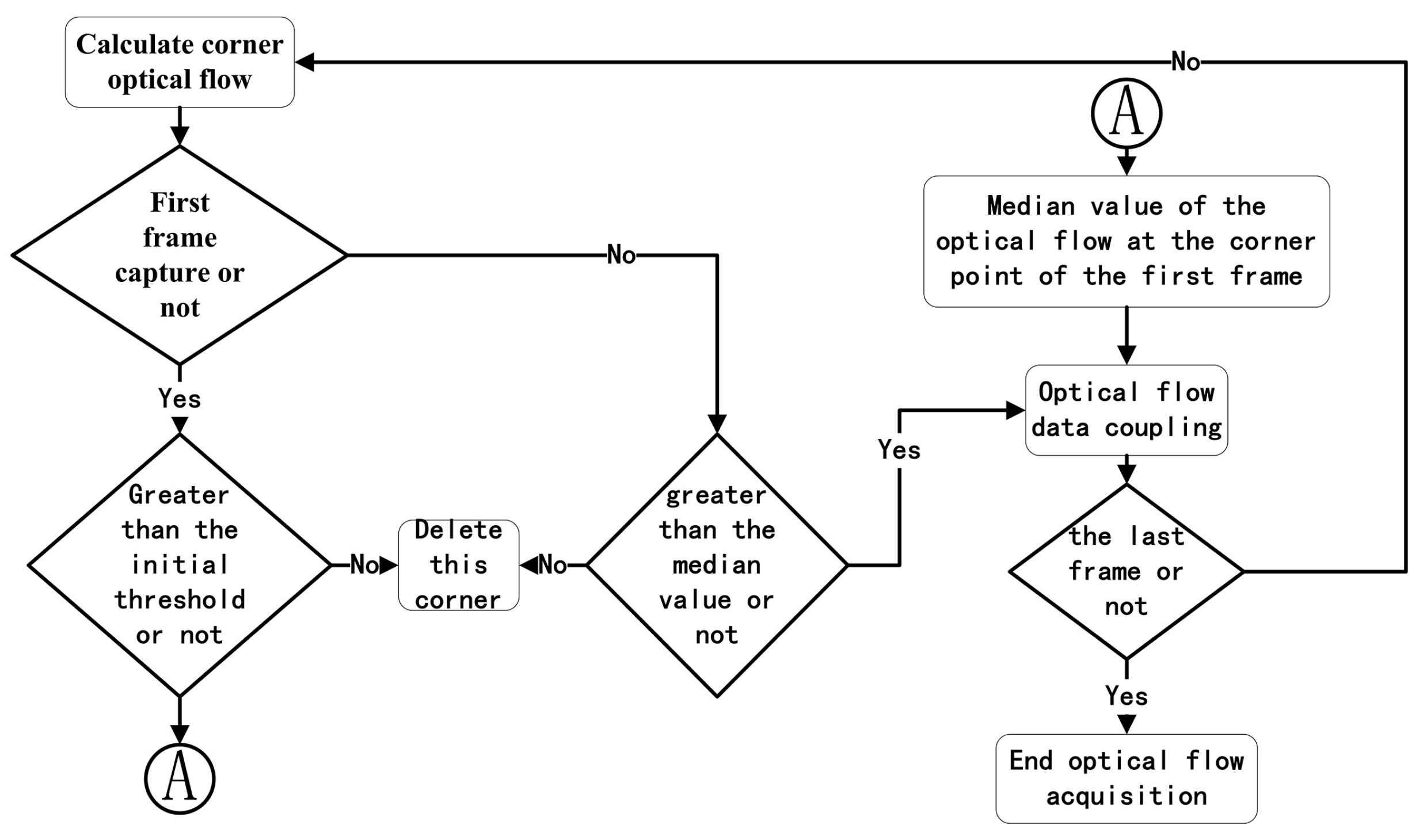
2.2.2. Dynamic Screening of Median Value
To accommodate optical flow acquisition for each flow state, a dynamic threshold corner screening method is necessary. By examining the collected optical flow reference parameters and utilizing the median value of the dynamic screening method, corner screening can automatically adjust to the optical flow acquisition of videos with varying flow rates and regimes. The following comparative experiments demonstrate that the collected optical flow data can furnish dependable gas–liquid two-phase flow information for the learning model. The flow of the median screening method is depicted in Figure 6.
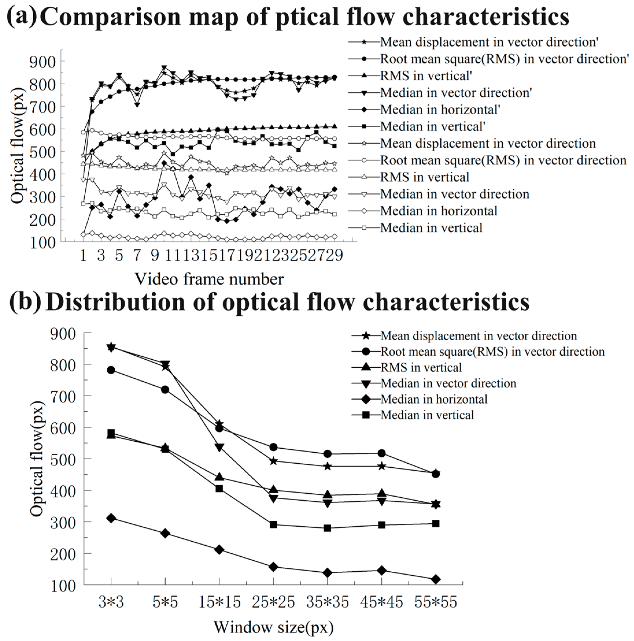
Experiments were conducted using a 5 × 5 window to assess the utilization of the median value sifting method for optical flow acquisition on the aforementioned 30 frames of video. Additionally, the results are illustrated in Figure 7.
In Figure 7, the values in the legend with ‘represent the values obtained by using the median screening method, while those without’ denote the values obtained without employing the median screening method. The median value obtained using the median screening method closely aligns with its average angular displacement, and its RMS remains consistently stable. This is particularly pronounced with regard to the vertical RMS value. Moreover, there is a strong correlation between the RMS value and the median value. Conversely, the difference between the median value and the root mean square obtained without the median screening method is more pronounced, indicating that a majority of the optical flow acquisition values are smaller, resulting in a more dispersed distribution and an increased presence of interfering angular points. Comparing the values obtained under different window sizes without median screening reveals that, after employing median screening, the median and RMS values exhibit greater similarity, especially in smaller windows, demonstrating that the optical flow calculation is more reasonable. The median value screening effectively filters out interfering corners, thereby enhancing the stability of the optical flow extraction and flow correlation. As a result, this approach contributes to enhanced stability in subsequent feature extraction and the accuracy of machine learning calculations.
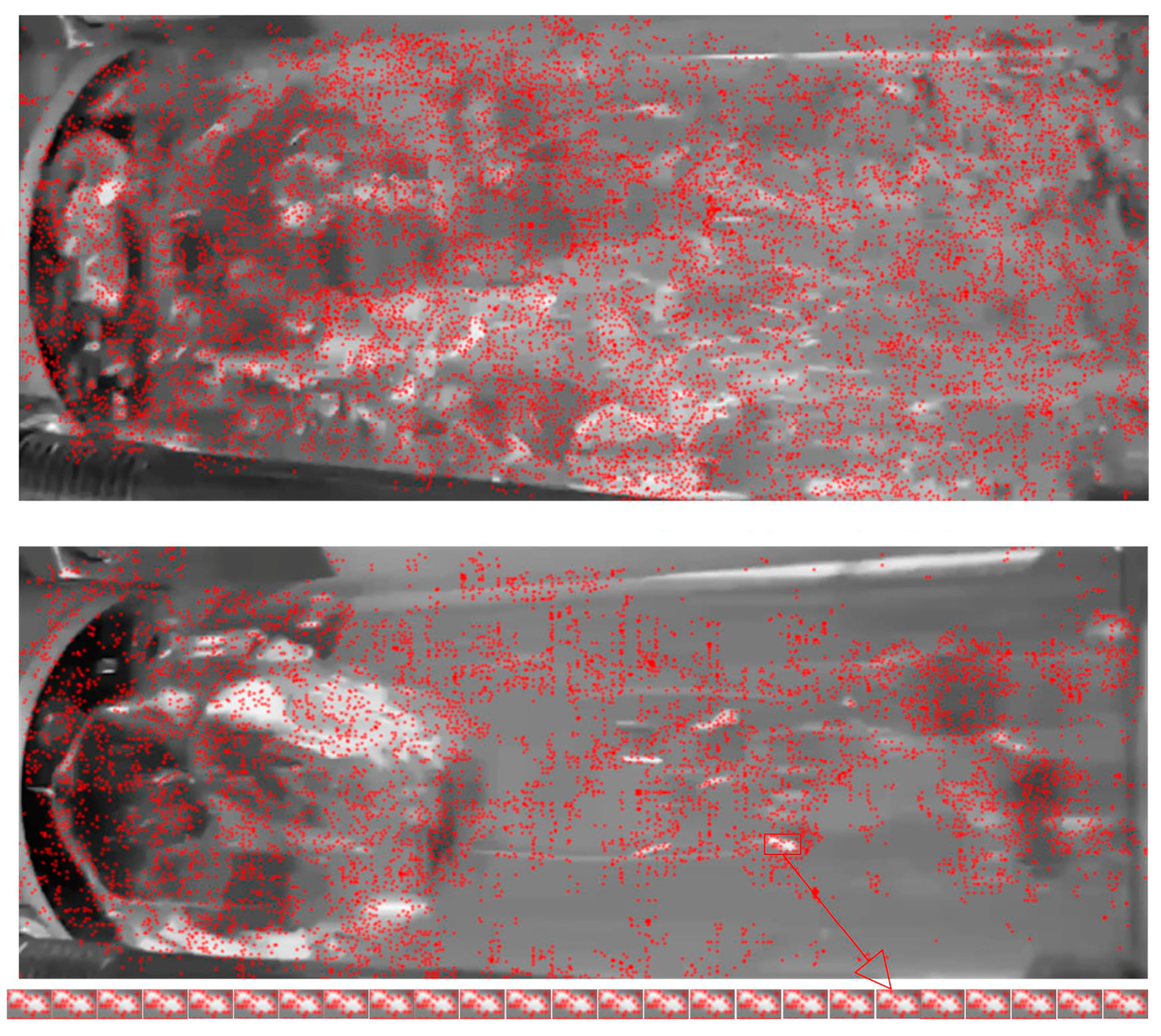
The results of corner point distribution after using and not using dynamic screening via the median method are shown in Figure 8.
Figure 8 illustrates the corner points obtained with and without the dynamic screening of the median method. Figure 8a shows corner points obtained without dynamic screening of the median method, while Figure 8b displays the corner points obtained with this method applied. The images reveal that, due to the density disparity between the gas and liquid phases, the light source experiences reflection at the interface, generating regions with notable grayscale changes. These corner points predominantly manifest at the interface between the gas and liquid phases, with their grayscale variations directly indicating the flow state of the two phases. Furthermore, there exists a specific correlation between the distribution of corner points and the reflection pattern of the light source. Through comparative analysis, it was observed that the corner point screening algorithm demonstrates a robust anti-interference capability. It effectively eliminates most corner points in the interference areas while also filtering out some random erroneous corner points in the flow region, thereby ensuring data accuracy and reliability.
2.2.3. Optical Flow Coupling
The proposed method for acquiring motion information in the video provides the positional information of corner points before and after two frames, denoted as (x1, y1) and (x2, y2), respectively. However, due to the varying number of corner points and optical flow across different flow patterns, these data cannot be directly utilized as the input for the optical flow machine learning model. Instead, it is necessary to couple the optical flow to generate useful feature information.
The proposed coupling methods are as follows:
where represents the average sum of squares of displacements per frame, is the average sum of squares of corner displacements per frame, denotes the open root of the sum of squares of the average displacements per frame, is the open root of the sum of squares of the average corner displacements per frame,
is the average corner displacement, and is the average corner displacement per frame. Moreover, n represents the number of frames of the video, and t is the total number of corners in the video captured by the pyramid L–K optical flow method. After data organization, 18 features in the x, y, and z directions are obtained, where z represents the vector direction. Along with the median value in the z direction, the median value in the y direction, the number of angular points per frame t/n, and the gas–liquid ratio, there are a total of 22-dimensional features, which are used as input features for the fitting of the machine learning regression model.
2.2.4. Feature Engineering
This research employs variance selection for feature filtering. A smaller variance of a particular feature indicates that the feature is consistent across samples and contains fewer distinguishing characteristics. To avoid interference from some irrelevant features during model training, a variance threshold was set to filter out features with variances below this threshold. This process helps in achieving more satisfactory results [32].
where represents the variance, denotes the number of video clips, denotes the value of the ith video clip on the feature, and is the mean value of the feature.
With the normalization method, the features are mapped to a distribution within the interval [0, 1] using Equation (20), removing variations in the degree of variability among the variables [33].
where represents the value of after max min normalization; denotes the value of the i-th video clip across the features; and denote the minimum and maximum values of the value of the ith video clip across all features, respectively.
2.2.5. Model Selection
The selected regression models for fitting the two-phase flow are random forest (RF) [34], support vector regression (SVR) [35,36], nearest neighbor regression (KNN) [37,38], multi-layer perceptron (MLP) [39], and gradient boosted regression (GBR) [40]. Parameter tuning for each model is performed using the grid search method.
In the training process, 5-fold cross-validation was used to evaluate the performance of the model [41]. The evaluation of the models is conducted using four metrics: RMSE, mean absolute error (MAE), MAPE, and the coefficient of determination (R2), which are calculated using the following equations:
where n denotes the number of video clips, represents the true value of traffic for the ith video clip, is the traffic measurements derived by the model through the ith video clip, SSR is the regression sum of squares, and SST is the total sum of squares.
3. Results
In this section, the RMSE, MAE, MAPE, and R2 provided in the figure and table illustrate the measurement accuracy and the stability of the model. Additionally, the proposed split comparison model measurement effectively reduces measurement errors.
3.1. Model Evaluation and Measurement Accuracy
Table 1 demonstrates the measurement accuracy and the validity of the machine learning model.
Table 1 indicates that the coefficients of determination (R2) for RF, SVR, KNN, and MLP all exceed 0.8, demonstrating the strong explanatory power of the prediction model for the features extracted from the two-phase flow video using pyramid L–K optical flow. This observation indicates the capability of the model to predict the two-phase flow rate, based on optical flow features. The RMSE reaches 1.83 m3/h, while the MAE reaches up to 1.37 m3/h. Notably, the GBR model emerges as the optimal choice with an R2 of up to 0.90, demonstrating a high level of goodness of fit and the ability to explain 90% of the data in the test set. Furthermore, the GBR model exhibits lower RMSE (1.32 m3/h) and MAE (0.92 m3/h) than the other models.
The predicted values from the best performing model are contrasted with the experimental true values, as depicted in Figure 9.
In Figure 9a, the horizontal coordinates represent the true values, while the vertical coordinates represent the predicted values. The proximity of the points to the diagonal line indicates a closer alignment between predicted and true values. The scatter represents the flow rate fitted to the test set. This figure illustrates the model prediction results for the test set, where 78.9% of the training set predictions fall within the 20% error line, with some individual values exhibiting larger fitting errors.
In Figure 9b, the results of the test set fitting generally align with the real values. It is worth noting that certain values are predicted to be high for low flow rates, while for large-flow values, predictions are lower. This discrepancy may be attributed to the significant variance in flow states within the gas–liquid two-phase flow. The substantial variability between small and large-flow rates results in considerable inconsistency within the dataset. It should be noted that machine learning models require a consistent distribution of training data, and such significant differences may lead to large errors.
3.2. Split_Comparison (SC) Model
The complexity of gas–liquid two-phase flow results in significant errors in individual flow predictions. To address this issue, this research introduces a Split Comparison (SC) model. This model comprises the optimal model GBR, designated as the preset measurement model GBR_A. Flow values of the test set are predicted using the optimal model as the benchmark. The test data are subsequently divided into two categories: large-flow data exceeding a predefined threshold and small-flow data below the threshold. In this study, to ensure a balanced representation of large and small-flow data, and considering the data distribution variances observed in Figure 9, a threshold of 5 m3/h is employed. The original dataset is then split into 93 large-flow and 93 small-flow data points. The large-flow data exceeding the threshold are utilized as training data for the large-flow model (GBR_B), while the small-flow data are used to train the small-flow model (GBR_C). GBR_B and GBR_C are utilized to predict the respective data segments in the test set, and the final result is derived by integrating the predictions from GBR_A, GBR_B, and GBR_C. The block diagram of this process is presented in Figure 10.
The measured data are generated by combining the results of GBR_A, GBR_B, and GBR_C. The SC model output represents the result with the minimum absolute error among the current datasets.
GBR_A models are trained and tested using the training dataset and the test dataset, respectively. The predictions of GBR_A on the test dataset are divided into test_H and test_S based on the threshold output. Subsequently, re-predictions are conducted using GBR_B and GBR_C. The test results of the three models are summarized in Table 2.
The model evaluation results indicate that the GBR_B model achieves superior prediction accuracy for larger flow rates, whereas the GBR_C model exhibits less accuracy for smaller flow rates. This is possibly due to the fact that the GBR_B model is better suited for predicting larger flows, whereas changes in flow state resulting from minor flow variations are less evident. Despite this, the GBR_C model still outperforms the overall predictions of GBR_A, and its results are relatively more consistent.
By comparing and computing the prediction outcomes of the three models, the selected prediction values based on absolute error are utilized to generate the final output of the SC model after assessment in Figure 11.
Table 3 presents a comparison of the precision between the GBR model and the SC model implementation.
As depicted in Figure 10 and Table 3, the SC model demonstrates enhanced corrective capabilities over the GBR model through its partitioning approach. The MAPE decreased from 17.2% to 8.0%, R2 increased by 0.07, RMSE decreased by 0.58 m3/h, and MAE decreased by 0.4 m3/h. These results demonstrate that the SC model notably enhances the prediction accuracy of the GBR model.
4. Discussion
In this study, due to limitations in sample size and validation attitude, only a limited amount of data was passed to verify the validity. In future research, enhancing the length of the observation line, increasing the number of collected pixels, and raising the frequency of collection can aid in feature extraction using the pyramid L–K photofluidic method. This approach can mitigate data errors caused by noisy corner points, expand the sample size, and enhance the measurement accuracy of the model.
5. Conclusions
This paper introduces an intelligent measurement system that integrates the pyramid L–K optical flow method and the Split Comparison (SC) model for gas–liquid two-phase flow rate measurement. Utilizing a camera positioned outside a vertical pipeline to capture flow videos, the pyramid L–K optical flow method gathers information about the gas–liquid two-phase flow. A median value screening method effectively eliminates noise from corner points, stabilizing the optical flow results. By coupling optical flow calculations, the obtained results serve as feature variables inputted into a machine learning model, enabling the combination of the pyramid L–K optical flow method and the machine learning model for gas–liquid two-phase flow rate measurement. To resolve the challenge of model generalization difficulty arising from significant flow rate distribution differences in the dataset, the model undergoes optimization via a Split Comparison (SC) approach. Results indicate that the SC model demonstrates notable improvements, with R2 increasing from 0.90 to 0.97, RMSE decreasing from 1.32 m3/h to 0.74 m3/h (representing 4.63% of the full range), MAE decreasing from 0.92 m3/h to 0.52 m3/h, and MAPE decreasing from 17.2% to 8.0%. This approach enables the convenient and reliable measurement of gas–liquid two-phase flow rates. It can handle complex flow conditions, obviates the need for cumbersome sensor installation and maintenance, enhances measurement robustness and convenience, reduces measurement costs, and offers a novel perspective for gas–liquid two-phase flow rate measurements.
Author Contributions
Conceptualization, J.W.; methodology, J.W.; software, J.W.; validation, J.W.; formal analysis, J.W.; investigation, Y.X.; resources, Y.X.; data curation, J.W. and Y.X.; writing—original, J.W.; writing—review and editing, D.X.; visualization, Z.H. and Y.X.; supervision, Z.H.; project administration, Z.H.; funding acquisition, Z.H. All authors have read and agreed to the published version of the manuscript.
Funding
This research was funded by the Science and Technology Department of Zhejiang Province, grant number 2022C01244.
Institutional Review Board Statement
Not applicable.
Informed Consent Statement
Not applicable.
Data Availability Statement
The raw data supporting the conclusions of this article will be made available by the authors upon request.
Conflicts of Interest
The authors declare no conflicts of interest.
Abbreviation
| Nomenclature | |
| A | Substitute Function, 5 × 5 Dimensions |
| B | Substitute Function, 5 × 5 Dimensions |
| C | Substitute Function, 5 × 5 Dimensions |
| D | Optical flow Coupling Function |
| d | Optical Flow Estimate, px |
| E | Grayscale Change Function |
| g | Initial Optical Flow |
| I | Grayscale Size |
| K | Response Coefficient |
| L | Pyramid Levels |
| R | Harris Response Value |
| t | Time, s |
| u | Optical Flow Vector, px |
| v | Optical Flow Vector, px |
| w | Window Weight Function, 5 × 5 Dimensions |
| x | Coordinates |
| y | Coordinates |
| z | Coordinates |
| Grayscale Change Function, 5 × 5 Dimensions | |
| Subscripts | |
| i | Unitnumber |
| k | Unitnumber |
| n | Unitnumber |
| min | Minimum |
| max | Maximum |
| qx | Represents the average sum of squares of displacements per frame, px |
| qtx | Average sum of squares of corner displacements per frame, px |
| qrx | Open root of the sum of squares of the average displacements per frame, px |
| qrtx | Open root of the sum of squares of the average corner displacements per frame, px |
| tx | Average corner displacement per frame, px |
| Acronyms | |
| RMSE | Root Mean Square Error |
| MAE | Mean Absolute Error |
| R2 | Coefficient of Determination |
| RF | Random Forest |
| SVR | Support Vector Regression |
| KNN | Nearest Neighbor Regression |
| MLP | Multi-Layer Perceptron |
| GBR | Gradient Boosted Regression |
| SC | Split Comparison |
References
- Paolinelli, L.D.; Nesic, S. Calculation of mass transfer coefficients for corrosion prediction in two-phase gas-liquid pipe flow. Int. J. Heat Mass Transf. 2021, 16, 120689. [Google Scholar] [CrossRef]
- Yang, L.; Chen, X.; Huang, C.; Liu, S.; Ning, B.; Wang, K. A review of gas-liquid separation technologies: Separation mechanism, application scope, research status, and development prospects. Chem. Eng. Res. Des. 2024, 201, 257–274. [Google Scholar] [CrossRef]
- Tan, C.; Murai, Y.; Liu, W.; Tasaka, Y.; Dong, F.; Takeda, Y. Ultrasonic Doppler Technique for Application to Multiphase Flows: A Review. Int. J. Multiph. Flow 2021, 144, 103811. [Google Scholar] [CrossRef]
- Zhao, Z.; Zhao, N.; Li, X.; Zhu, Y.; Fang, L.; Li, X.; Guo, L.; Li, C. The Gas-Liquid Flow Rate Measurement Based on Multisensors and Machine Learning. IEEE Sens. J. 2022, 22, 17234–17242. [Google Scholar] [CrossRef]
- Li, S.; Bai, B. Gas-liquid two-phase flow rates measurement using physics-guided deep learning. Int. J. Multiph. Flow 2023, 162, 104421. [Google Scholar] [CrossRef]
- Li, S.; Bai, B. Gas–liquid intermittent flow rates measurement based on two-phase mass flow multiplier and neural network. Meas. Sci. Technol. 2021, 32, 105306. [Google Scholar] [CrossRef]
- Hu, D.; Li, J.; Liu, Y.; Li, Y. Flow Adversarial Networks: Flowrate Prediction for Gas–Liquid Multiphase Flows Across Different Domains. IEEE Trans. Neural Netw. Learn. Syst. 2020, 31, 475–487. [Google Scholar] [CrossRef] [PubMed]
- Gao, Z.-K.; Liu, M.-X.; Dang, W.-D.; Cai, Q. Multitask-Based Temporal-Channelwise CNN for Parameter Prediction of Two-Phase Flows. IEEE Trans. Ind. Inform. 2021, 17, 6329–6336. [Google Scholar] [CrossRef]
- Gao, Z.; Li, M.; Hou, L.; Deng, H.; Xu, W.; Dang, W.; Deng, G. Stage-Wise Densely Connected Network for Parameter Measurement of Two-Phase Flows. IEEE Sens. J. 2021, 16, 18123–18131. [Google Scholar] [CrossRef]
- Zhang, J.; Wei, X.; Wang, Z. The Recognition Algorithm of Two-Phase Flow Patterns Based on GoogLeNet+5 CoordAttention. Micromachines 2023, 14, 462. [Google Scholar] [CrossRef]
- Nie, F.; Wang, H.; Song, Q.; Zhao, Y.; Shen, J.; Gong, M. Image identification for two-phase flow patterns based on CNN algorithms. Int. J. Multiph. Flow 2022, 152, 104067. [Google Scholar] [CrossRef]
- Gao, Z.; Qu, Z.; Cai, Q.; Hou, L.; Li, M.; Yuan, T. A Deep Branch-Aggregation Network for Recognition of Gas–Liquid Two-Phase Flow Structure. IEEE Trans. Instrum. Meas. 2021, 70, 1–8. [Google Scholar] [CrossRef]
- Gao, Z.-K.; Liu, M.-X.; Dang, W.-D.; Cai, Q. A novel complex network-based deep learning method for characterizing gas–liquid two-phase flow. Pet. Sci. 2021, 18, 259–268. [Google Scholar] [CrossRef]
- Kadish, S.; Schmid, D.; Son, J.; Boje, E. Computer Vision-Based Classification of Flow Regime and Vapor Quality in Vertical Two-Phase Flow. Sensors 2022, 22, 996. [Google Scholar] [CrossRef]
- Kuang, B.; Nnabuife, S.G.; Sun, S.; Whidborne, J.F.; Rana, Z.A. Gas-liquid flow regimes identification using non-intrusive Doppler ultrasonic sensor and convolutional recurrent neural networks in an s-shaped riser. Digit. Chem. Eng. 2022, 22, 100012. [Google Scholar] [CrossRef]
- OuYang, L.; Jin, N.; Ren, W. A new deep neural network framework with multivariate time series for two-phase flow pattern identification. Expert Syst. Appl. 2022, 205, 117704. [Google Scholar] [CrossRef]
- Ooi, Z.J.; Zhu, L.; Bottini, J.L. Brooks. Identification of flow regimes in boiling flows in a vertical annulus channel with machine learning techniques. Int. J. Heat Mass Transf. 2022, 185, 122439. [Google Scholar] [CrossRef]
- Nnabuife, S.G.; Kuang, B.; Whidborne, J.F.; Rana, Z. Non-intrusive classification of gas-liquid flow regimes in an S-shaped pipeline riser using a Doppler ultrasonic sensor and deep neural networks. Chem. Eng. J. 2021, 403, 126401. [Google Scholar] [CrossRef]
- Nnabuife, S.G.; Kuang, B.; Whidborne, J.F.; Rana, Z.A. Development of Gas–Liquid Flow Regimes Identification Using a Noninvasive Ultrasonic Sensor, Belt-Shape Features, and Convolutional Neural Network in an S-Shaped Riser. IEEE Trans. Cybern. 2023, 53, 3–17. [Google Scholar] [CrossRef]
- Arteaga-Arteaga, H.B.; Mora-Rubio, A.; Florez, F.; Murcia-Orjuela, N.; Diaz-Ortega, C.E.; Orozco-Arias, S.; dela Pava, M.; Bravo-Ortíz, M.A.; Robinson, M.; Guillen-Rondon, P.; et al. Machine learning applications to predict two-phase flow patterns. PeerJ Comput. Sci. 2021, 7, 798. [Google Scholar] [CrossRef]
- Wajman, R.; Nowakowski, J.; Łukiański, M.; Banasiak, R. Machine learning for two-phase gas-liquid flow regime evaluation based on raw 3D ECT measurement data. Bull. Pol. Acad. Sci. 2024, 72, 148842. [Google Scholar] [CrossRef]
- Zhang, L.; Zhang, S. Gas/Liquid Two-Phase Flow Pattern Identification Method Using Gramian Angular Field and Densely Connected Network. IEEE Sens. J. 2023, 23, 4022–4032. [Google Scholar] [CrossRef]
- Chen, H.; Dang, Z.; Park, S.S.; Hugo, R. Robust CNN-based flow pattern identification for horizontal gas-liquid pipe flow using flow-induced vibration. Exp. Therm. Fluid Sci. 2023, 148, 11097. [Google Scholar] [CrossRef]
- Hafsa, N.; Rushd, S.; Yousuf, H. Comparative Performance of Machine-Learning and Deep-Learning Algorithms in Predicting Gas–Liquid Flow Regimes. Processes 2023, 11, 177. [Google Scholar] [CrossRef]
- Dukler, A.E.; Taitel, Y. Flow Pattern Transitions in Gas-Liquid Systems: Measurement and Modeling. In Multiphase Science and Technology; Hewitt, G.F., Delhaye, J.M., Zuber, N., Eds.; Springer: Berlin/Heidelberg, Germany, 1986; pp. 1–94. [Google Scholar] [CrossRef]
- Lucas, B.D.; Kanade, T. An iterative image registration technique with an application to stereo vision. Proc. DARPA Image Understand. Workshop 1981, 81, 121–130. [Google Scholar]
- Zhong, L.; Meng, L.; Hou, W.; Huang, L. An Improved Visual Odometer Based on Lucas-Kanade Optical Flow and ORB Feature. IEEE Access 2023, 11, 47179–47186. [Google Scholar] [CrossRef]
- Niu, Y.; Xu, Z.; Che, X. Dynamically Removing False Features in Pyramidal Lucas-Kanade Registration. IEEE Trans. Image Process. 2014, 23, 3535–3544. [Google Scholar] [CrossRef] [PubMed]
- Al-Qudah, S.; Yang, M. Large Displacement Detection Using Improved Lucas–Kanade Optical Flow. Sensors 2023, 23, 3152. [Google Scholar] [CrossRef]
- Morevec, H.P. Towards automatic visual obstacle avoidance. In Proceedings of the International Joint Conference on Artificial Intelligence, Cambridge, MA, USA, 22–25 August 1977; p. 584. [Google Scholar]
- Harris, C.G.; Stephens, M.J. A combined corner and edge detector. Proc. Alvey Vis. Conf. 1988, 1988, 147–151. [Google Scholar]
- Batur, D.; Choobineh, F.F. Mean-variance based ranking and selection. Proc. 2010 Winter Simul. Conf. 2010, 10, 1160–1166. [Google Scholar]
- Rana, P.; St-Onge, B.; Prieur, J.-F.; Budei, B.C.; Tolvanen, A.; Tokola, T. Effect of feature standardization on reducing the requirements of field samples for individual tree species classification using ALS data. ISPRS J. Photo-Grammetry Remote Sens. 2022, 184, 189–202. [Google Scholar] [CrossRef]
- Dong, L.-J.; Li, X.-B.; Peng, K. Prediction of rockburst classification using Random Forest. Trans. Nonferr. Met. Soc. China 2013, 23, 472–477. [Google Scholar]
- Zhang, Z.; Ding, S.; Sun, Y. MBSVR: Multiple birth support vector regression. Inf. Sci. 2021, 552, 65–79. [Google Scholar] [CrossRef]
- Ni, N.; Chan, C. Identification and measurement of gas mixture by using the support vector regression technique. Meas. Sci. Technol. 2009, 20, 115601. [Google Scholar] [CrossRef]
- Atanasovski, M.; Kostov, M.; Arapinoski; Spirovski, M. K-Nearest Neighbor Re-gression for Forecasting Electricity Demand. International Scientific Conference on Information. In Proceedings of the 2020 55th International Scientific Conference on Information, Communication and Energy Systems and Technologies (ICEST), Niš, Serbia, 10–12 September 2020; pp. 110–113. [Google Scholar] [CrossRef]
- Assi, K.C.; Labelle, H.; Cheriet, F. Modified Large Margin Nearest Neighbor Metric Learning for Regression. IEEE Signal Process. Lett. 2014, 21, 292–296. [Google Scholar] [CrossRef]
- Makalic, E.; Allison, L. MMLD Inference of Multilayer Perceptrons. In Algorithmic Probability and Friends. Bayesian Prediction and Artificial Intelligence; Dowe, D.L., Ed.; Lecture Notes in Computer Science; Springer: Berlin/Heidelberg, Germany, 2013; Volume 7070, pp. 261–272. [Google Scholar] [CrossRef]
- Yamagishi, J.; Kawai, H.; Kobayashi, T. Phone duration modeling using gradient tree boosting. Speech Commun. 2008, 50, 405–415. [Google Scholar] [CrossRef]
- Fushiki, T. Estimation of prediction error by using K-fold cross-validation. Stat. Comput. 2011, 21, 137–146. [Google Scholar] [CrossRef]
Figure 1.
Schematic diagram of the experimental setup.

Figure 2.
Flow patterns of two-phase flows during the experiment.

Figure 3.
Flow measurement flowchart.

Figure 4.
Distribution of the optical flow characteristics.

Figure 5.
Comparison map of a dynamic threshold corner screening method.

Figure 6.
Flowchart of the median value screening.

Figure 7.
Optical flow characteristics of the median value using the sieving method.

Figure 8.
Corner point selection effect of dynamic screening of the median method.

Figure 9.
Distribution of prediction results using different models.

Figure 10.
Block diagram of the split comparison modeling system.

Figure 11.
The test results obtained using the SC model.


Table 1.
Regression model evaluation table.
| Evaluation Indicators | RF | SVR | KNN | MLP | GBR |
|---|---|---|---|---|---|
| RMSE (m3/h) | 1.58 | 1.83 | 1.70 | 1.75 | 1.32 |
| MAE (m3/h) | 1.23 | 1.24 | 1.37 | 1.17 | 0.92 |
| R2 | 0.85 | 0.80 | 0.83 | 0.82 | 0.90 |
| MAPE (%) | 24.6 | 35.1 | 26.6 | 32.7 | 17.2 |
Table 2.
The performance measures of different models.
| Model Name | RMSE (m3/h) | MAE (m3/h) | R2 | MAPE% |
|---|---|---|---|---|
| GBR_A | 1.23 | 0.86 | 0.91 | 16.7% |
| GBR_B | 0.94 | 0.77 | 0.87 | 8.2% |
| GBR_C | 0.55 | 0.44 | 0.74 | 16.4% |
Table 3.
The prediction results obtained from the SC model.
| Model Name | RMSE (m3/h) | MAE (m3/h) | R2 | MAPE (%) |
|---|---|---|---|---|
| GBR | 1.32 | 0.92 | 0.90 | 17.2 |
| SC | 0.74 | 0.52 | 0.97 | 8.0 |
Disclaimer/Publisher’s Note: The statements, opinions and data contained in all publications are solely those of the individual author(s) and contributor(s) and not of MDPI and/or the editor(s). MDPI and/or the editor(s) disclaim responsibility for any injury to people or property resulting from any ideas, methods, instructions or products referred to in the content. |
© 2024 by the authors. Licensee MDPI, Basel, Switzerland. This article is an open access article distributed under the terms and conditions of the Creative Commons Attribution (CC BY) license (https://creativecommons.org/licenses/by/4.0/).
Share and Cite
MDPI and ACS Style
Wang, J.; Huang, Z.; Xu, Y.; Xie, D. Gas–Liquid Two-Phase Flow Measurement Based on Optical Flow Method with Machine Learning Optimization Model. Appl. Sci. 2024, 14, 3717. https://doi.org/10.3390/app14093717
AMA Style
Wang J, Huang Z, Xu Y, Xie D. Gas–Liquid Two-Phase Flow Measurement Based on Optical Flow Method with Machine Learning Optimization Model. Applied Sciences. 2024; 14(9):3717. https://doi.org/10.3390/app14093717
Chicago/Turabian StyleWang, Junxian, Zhenwei Huang, Ya Xu, and Dailiang Xie. 2024. "Gas–Liquid Two-Phase Flow Measurement Based on Optical Flow Method with Machine Learning Optimization Model" Applied Sciences 14, no. 9: 3717. https://doi.org/10.3390/app14093717
Note that from the first issue of 2016, this journal uses article numbers instead of page numbers. See further details here.