Article

A Novel Mechanical Fault Diagnosis Scheme Based on the Convex 1-D Second-Order Total Variation Denoising Algorithm

The Key Laboratory of Metallurgical Equipment and Control of Education Ministry, Wuhan University of Science and Technology, Wuhan 430081, China
*
Author to whom correspondence should be addressed.
Appl. Sci. 2016, 6(12), 403; https://doi.org/10.3390/app6120403
Submission received: 26 October 2016 / Revised: 21 November 2016 / Accepted: 29 November 2016 / Published: 2 December 2016
(This article belongs to the Special Issue Structural Health Monitoring (SHM) of Civil Structures)

Abstract

:
Convex 1-D first-order total variation (TV) denoising is an effective method for eliminating signal noise, which can be defined as convex optimization consisting of a quadratic data fidelity term and a non-convex regularization term. It not only ensures strict convex for optimization problems, but also improves the sparseness of the total variation term by introducing the non-convex penalty function. The convex 1-D first-order total variation denoising method has greater superiority in recovering signals with flat regions. However, it often produces undesirable staircase artifacts. Moreover, actual denoising efficacy largely depends on the selection of the regularization parameter, which is utilized to adjust the weights between the fidelity term and total variation term. Using this, algorithms based on second-order total variation regularization and regularization parameter optimization selection are proposed in this paper. The parameter selection index is determined by the permutation entropy and cross-correlation coefficient to avoid the interference by human experience. This yields the convex 1-D second-order total variation denoising method based on the non-convex framework. Comparing with traditional wavelet denoising and first-order total variation denoising, the validity of the proposed method is verified by analyzing the numerical simulation signal and the vibration signal of fault bearing in practice.

Graphical Abstract

1. Introduction

Rolling bearing is widely used in rotating machinery, and its operating status directly affects the safety and stable operation of the entire device, and even the whole production line. The failure rate of bearing is relatively high in the actual process of mechanical equipment. Thus, fault identification of bearing state has great significance in mechanical fault diagnosis [1,2]. To date, the detection of bearing failure is mostly based on vibration signal processing. The main goal is to improve the identification accuracy on the fault characteristic frequency from the original vibration signal [3], and one of important research objectives aims to reduce the noise component and improve the signal-to-noise ratio (SNR).
The traditional denoising method primarily uses different filtering algorithm for noise reduction, which is based on the different frequency characteristic distribution of the useful signals and unwanted signals such as noisy data. Time-frequency analysis is widely utilized in stationary and periodicity signal analysis [4]. However, it cannot completely detect the useful information contained in the original measurement signal. In particular, the mechanical equipment fault signal has tended to be non-stationary, non-linear, and non-Gaussian [5]. Therefore, there are some disadvantages for traditional denoising methods in mechanical fault feature extraction. Many scholars have adopted the wavelet transform as a tool for denoising due to its good time-frequency localization ability, but it is restricted by proper choice of wavelet basis function and decomposition level [6,7]. Empirical mode decomposition (EMD) is a new non-stationary signal adaptive processing method, which has been widely used in one-dimensional signal processing [8]. However, this method also has some obvious shortcomings, such as lack of rigorous theoretical support, model-aliasing and the endpoint effect [9,10]. Moreover, some techniques have been heavily employed in fault diagnosis and fault reconstruction for a class of nonlinear systems [11,12]. Traditional total variation (TV) algorithm is another widely used signal processing method, especially in image processing and one-dimensional signal processing [13,14], because it can suppress noise effectively and maintain a good image edge. Commonly, TV algorithm is constituted by a quadratic data fidelity term and a convex regularization term [15]. Subsequently, novel convex 1-D total variation denoising was introduced by the fact that non-convex regularizers can better recover flat signal regions [16]. Therefore, the non-smooth convex regularizer is replaced by a non-convex one such as logarithmic penalty or arctangent penalty [17,18]. It is proven that convex 1-D total variation denoising has better capacity than the traditional total variation denoising method in signal reconstruction. Nevertheless, the regularization parameter is employed to adjust the weights between fidelity constraints and total variation term, which lack objective evaluation criteria. Furthermore, the abovementioned convex 1-D total variation (TV) denoising by the first-order total variation operator always produces undesirable staircase artifacts.
Since the second-order difference is sparser than the first-order difference, it has been widely applied in image processing [19,20]. In order to improve the performance of signal reconstruction and avoid the problem of staircase artifacts, the second-order total variation using non-convex penalty function is firstly employed for vibration signal processing in this paper. Then, this paper distinguishes the differences between unwanted signal such as noisy data and useful signals by permutation entropy in dynamics characters. The concept of permutation entropy (PE) was proposed in the application of measuring the complexity of one-dimensional time series [21]. It is an algorithm to describe irregular and nonlinear systems, which cannot be quantitatively described in a relatively simple way. The PE has the advantages of simple calculation and high sensitivity to signal change, which can be employed to evaluate the denoising effect [22,23]. Nevertheless, the phenomena of excessive noise reduction should be avoided, as it causes the details to be lost in the signal. Thus, the reconstructed signal must maintain a certain similarity with original signal, which can be described by cross-correlation coefficient. Therefore, regularization parameter optimization method is proposed based on permutation entropy and cross-correlation coefficient in this paper. It not only will be able to ensure the greatest degree of suppression noise, but also can improve the similarity between the signal after noise reduction and the original signal, which can avoid the problem of excessive denoising. In order to verify the rationality and feasibility of the proposed method, it is used to analyze the numerical simulation and the actual fault vibration signal of rolling bearings in the bearing test rig and the fan in metallurgical industry.
The rest of the paper is organized as follows. In Section 2, the basic ideas of convex 1-D second-order total variation denoising method are introduced. The simulation signal analysis is described in Section 3. The fault bearing data from bearing test rig is analyzed in Section 4. The industrial measurement signal analysis of faulty bearing in fan is illustrated in Section 5. The final conclusions are given in Section 6.

2. Theoretical Descriptions

2.1. The Basic Principle of Second-Order Total Variation Denoising Algorithm

Given that the original signal is expressed as x = [ x 0 , x 1 , x 2 , ... , x N 1 ] , where N is the length of original time series. Then, the bidiagonal matrix D 1 R ( n 1 ) × n is defined as:
D 1 = [ 1 1 1 1 1 1 ]
The expression of l p -Norm ( p 1 ) is as follows:
x p = ( x 1 p + x 2 p + + x N p ) 1 p
when p = 1 and p = 2 , Equation (2) can be presented as Equations (3) and (4), respectively.
x 1 = ( | x 1 | + | x 2 | + + | x N | )
x 2 = | x 1 | 2 + | x 2 | 2 + + | x N | 2
Then the first-order total variation term can be noted by Equation (5):
T V ( x ) = D 1 x 1 = n = 1 N 1 | x ( n ) x ( n 1 ) |
Since the traditional total variation using first-order difference has poor performance in signal reconstruction, the second-order total variation is introduced in this paper, which is defined in Equation (6).
T V 2 ( x ) = D 2 x 1 = n = 1 N 1 | x ( n + 2 ) 2 x ( n + 1 ) + x ( n ) |
In Equations (5) and (6), T V ( x ) and T V 2 ( x ) is represented as the operator of first-order and second-order total variation, respectively. Generally, the noisy signal y ( n ) was composed of useful signal x ( n ) in additive Gaussian white noise w ( n ) , which can be expressed as follows:
y ( n ) = x ( n ) + w ( n ) ( n = 0 , 1 , , N 1 )
Therefore, the one-dimensional second-order total variation denoising model can be attributed to the following convex optimization problem:
F ( x ) = arg min x 1 2 y x 2 2 + λ ϕ ( T V 2 ( x ) )
In Equation (8), F ( x ) is the objective function: R N R ; λ is the regularization parameter which is to control the degree of smoothing; ϕ : R R is a sparsity-promoting penalty function (regularizer). The second term in the expression reflects the degree of signal variation.

2.2. The Proposed Optimized Convex 1-D Second-Order Total Variation Denoising Algorithm

In the basic theory of traditional total variation denoising algorithm, enhanced sparsity penalty function is usually defined as ϕ ( x ) = x 1 . However, it has been proven that the non-convex penalties have more obvious advantages in signal reconstruction over convex penalties [16]. Therefore, it is necessary to introduce an appropriate enhanced sparsity penalty function ϕ ( x ) to improve the sparsity of T V 2 ( x ) and ensure the convexity of the objective function, which is conducive to solving the problem. Typical non-convex penalty functions should be continuous, symmetrical and twice differentiable. The most common non-convex penalty functions are the logarithmic penalty and arctangent penalty [17], which are shown in Equations (9) and (10):
ϕ ( x ; a ) = 1 a log ( 1 + a | x | )
ϕ ( x ; a ) = 2 a 3 ( tan 1 ( 1 + 2 a | x | 3 ) π 6 )
Considering the convexity condition, the parameter a should be selected in 0 < a < 1 4 λ .
After the identification of new sparsity upgrade penalty function ϕ ( x ) , this paper uses majorization-minimization (MM) approach to achieve fast convergence and Equation (11) is the basic iterative solver equation.
x ( k + 1 ) = y D 2 T ( 1 λ [ W ( D 2 x ( k ) ) ] 1 + D 2 D 2 T ) 1 D 2 y
where W ( D 2 x ) = ϕ ( D 2 x ) D 2 x , x ( 0 ) = y , k = 1 , ... , N . Generally, the number of iterations N is selected as 20, which are usually sufficient. Equation (11) indicates that the regularization parameter λ plays a very important role in iterative solution processes, which is directly related to the actual noise elimination effect. Therefore, the parameter λ optimization method is introduced based on permutation entropy and cross correlation in this paper. Permutation entropy (PE) was proposed to detect random time series and dynamics mutations. PE has a series of advantages: simple concept, fast computing speed, strong anti-interference ability and good robustness, especially in nonlinear data analysis. Given the time series x ( i ) ( i = 1 , 2 , ... , N ) its phase space is reconstructed to obtain Hankel matrix.
Y = ( x ( 1 ) x ( 1 + τ ) x ( 1 + ( m 1 ) τ ) x ( 2 ) x ( 2 + τ ) x ( 2 + ( m 1 ) τ ) x ( j ) x ( j + τ ) x ( j + ( m 1 ) τ ) x ( K ) x ( K + τ ) x ( K + ( m 1 ) τ ) )
where j = 1 , 2 , ... , K , m and τ are denoted as embedding dimension and delay time respectively, K = n ( m 1 ) τ . Each row in the matrix can be seen as a reconstruction component and there are K reconstruction components. The reconstructed matrix Y in each row { x ( j ) , x ( j + τ ) , ... , x ( j + ( m 1 ) τ ) } are rearranged in ascending order, and j 1 , j 2 , ... , j m indicate the index of each element in the column of reconstruction components, namely:
x ( i + ( j 1 1 ) τ ) x ( i + ( j 2 1 ) τ ) x ( i + ( j m 1 ) τ )
If there is an equal value in the reconstruction component such as x ( i + ( j p 1 ) τ ) = x ( i + ( j q 1 ) τ ) , the elements should be aligned according to the values of j p and j q . In other words, when j p < j q , we can obtain the following Equation:
x ( i + ( j p 1 ) τ ) x ( i + ( j q 1 ) τ )
A set of symbols sequence can be obtained for each row in the matrix Y .
S ( l ) = { j 1 , j 2 , , j m }
where l = 1, 2, …, k, and km!. There is a total of m! different symbol sequences {j1, j2, …, jm} in m dimensional phase space, and symbol sequence S ( l ) is just one of them. The probability of each symbol sequence was calculated and named as P1, P2, …, Pk. The permutation entropy (PE) of different symbol sequences in time series x ( i ) is defined by the form of information entropy:
H p ( d ) = j = 1 k P j In ( P j )
The value of H p ( d ) indicates the degree of randomness of time series. Namely, the larger value of H p ( d ) declares the greater randomness of time series, and vice versa. Therefore, the permutation entropy can be used to detect the randomness of time series. Naturally, the permutation entropy for random noise is large, while the permutation entropy of harmonic signal and the modulation signal is small.
From Equation (8), the convex 1-D second-order total variation denoising algorithm involves two parts, the former is fidelity constraint 1 2 y x 2 2 and the latter is the total variation term ϕ ( [ T V 2 ( x ) ] ) . It is worthy of mention that λ is used to adjust the weights. If λ = 0 , the total variation term has no difference in the punishment, and the obtained signal x is equal to the original signal y . Conversely, if λ tends to infinity, the total variation penalty term works and the fidelity will be poor, which may deviate from the original signal x to a great extent. It should be noted that a certain similarity between the signal after denoising and the original signal should be maintained to avoid the phenomenon of excessive noise reduction. Therefore, a new evaluation index for selecting parameter λ should be proposed to achieve balance in signal fidelity constraints and total variation term. To reasonably select parameters λ , this paper proposed a weighted index based on permutation entropy P E _ i n d e x and cross-correlation C _ i n d e x as a measurement of denoising result, which can be calculated by Equations (16) and (17), respectively.
C _ i n d e x = cov ( x , y ) σ x σ y = E ( ( x x ¯ ) ( y y ¯ ) ) σ x σ y
Consequently, the final index P E C _ i n d e x is determined as the ratio of the cross correlation coefficient and entropy arrangement in Equation (18). Basically, the larger value of P E C _ i n d e x always indicates better denoising result.
P E C _ i n d e x = max ( C _ i n d e x P E _ i n d e x )

3. Simulation Signal Analysis

3.1. The Role of Permutation Entropy on Signal Randomness Detection

The embedding dimension m and delay time τ should be determined in permutation entropy calculation firstly. Bandt [21] recommended that the embedding dimension m should be in the range of 3–7. If m is too small, the reconstructed vector contains very little state and the algorithm loses its meaning. If m is too large, the reconstruction phase space will homogenize the time series, which will not only extend the computation time, but will also be unable to reflect subtle changes in sequence. Thus, the parameter m = 6 is selected in this paper. Due to the fact that delay time τ has little impact on the operation sequence, τ = 1 is chosen here. To validate the effect of permutation entropy on signal random detection, the harmonic signal, modulation signal and Gaussian white noise signal were analyzed, respectively. The expressions of harmonic signal and modulation signal are listed as follows:
s 1 = sin ( 2 π f 1 t )
s 2 = [ 1 + 0.5 sin ( 2 π f 2 t ) ] sin ( 2 π f 3 t )
where N = 2048 , f 1 = 500 Hz, f 2 = 5 Hz, f 3 = 10 Hz. s 3 is the standard Gaussian white noise. According to the definition of arrangement entropy, the values of three simulated signals are chosen as 1.4429, 1.1938 and 6.3648, respectively. The result indicates that there is great difference among the permutation entropy values of noise signal, harmonic and modulation signal. Generally, the permutation entropy value of the noise signal is much larger than harmonic signal and modulated signal. Therefore, the permutation entropy can be used to effectively evaluate the actual denoising.

3.2. Numerical Simulation Analysis

Generally, vibration signal is composed of a modulation component and a noise component. Therefore, the simulation signal is generated to verify the effectiveness of the improved total variation denoising method, which is listed as follows.
x = x 1 + x 2
x 1 = sin ( 2 π f 1 t + cos ( 2 π f 2 t ) )
where x 1 is a typical modulating signal with f 1 = 15 Hz and f 2 = 30 Hz. x 2 is Gaussian white noise, its mean value is 0 and variance is δ = 0.5 . The clean signal x 1 and noisy signal x 2 are shown in Figure 1, respectively. It can be seen that the modulation characteristics of the original signal in noisy signal are difficult to identify in Figure 1. Using the preferred regularization parameter selection method based on the weights between permutation entropy and cross correlation coefficient defined in Equation (18), the parameter can be selected as λ = 1.3 .
To verify the validity of the different denoising methods, the performance is evaluated by signal-to-noise ratio (SNR). Comparing with the traditional wavelet denoising method and the typical total variation denoising method using first-order total variation, the proposed second-order total variation noise reduction method by non-convex penalty function defined in Equations (9) and (10) is used for simulation signal analysis. It is important to note that the ‘wden’ function is chosen as the automatic 1-D denoising function and the wavelet basis function is set as ‘sym5’ in wavelet denoising. Moreover, the wavelet basis function selection and parameter setting are the same in the remaining part of this paper. The analysis results provided by different methods are shown in Figure 2. We can make the conclusion that the proposed method can largely reduce the noise components from original signal and maintain the key characteristics to the greatest extent. The proposed improved total variation noise reduction method can acquire a larger value of SNR to 11.31 db under the condition of δ = 0.5 .
In order to evaluate the effect of different noise level for the simulated signal, we also calculate the SNR after denoising by different methods in Table 1. It can be seen that the proposed method has better noise reduction performance than other methods.

4. Experimental Verification

4.1. Experimental Setup

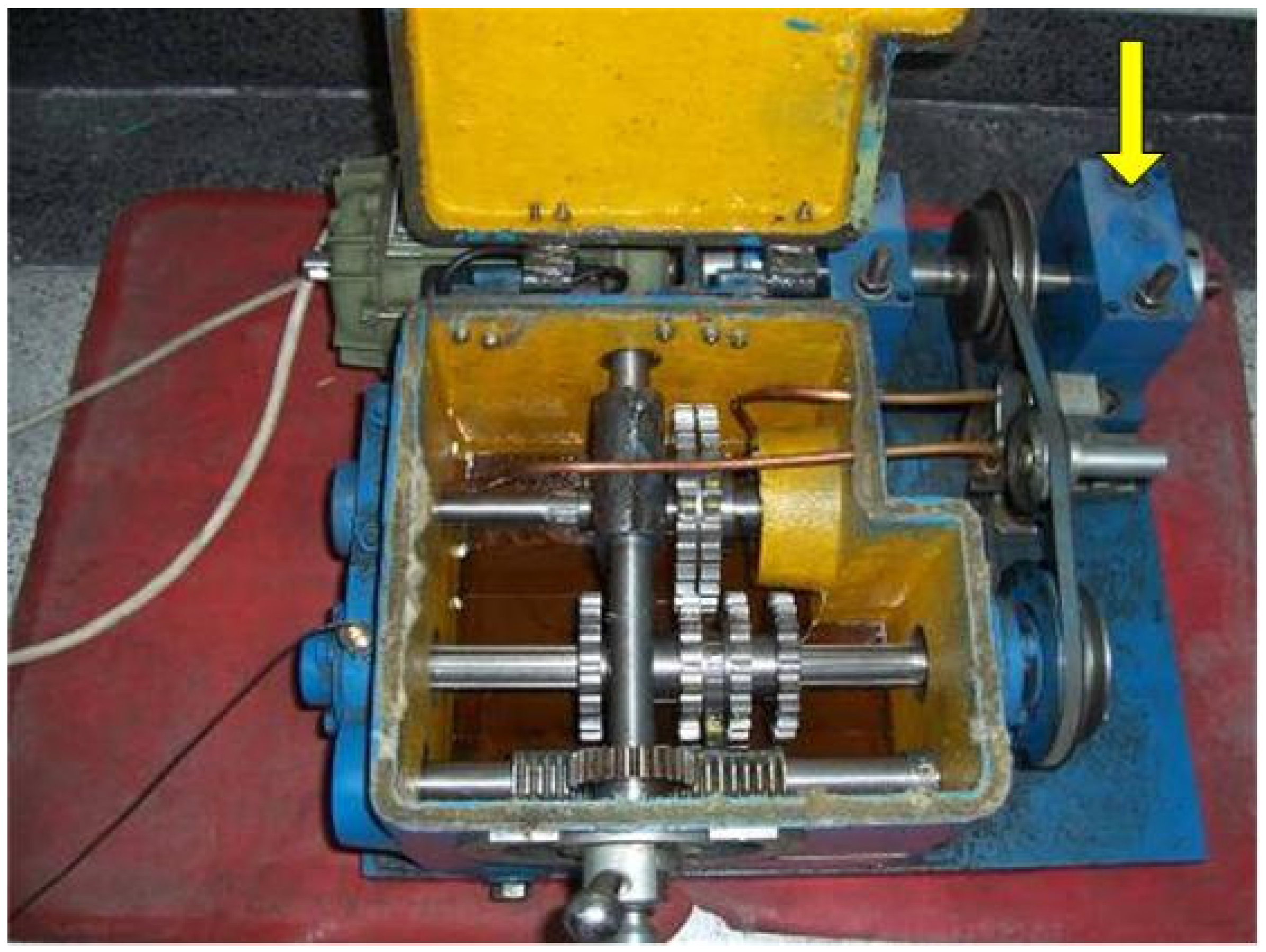
A great impact on production can be caused in actual operation when failure occurs in rolling bearing. The recognition of bearing failure mostly depends on bearing fault characteristic frequency extraction. In order to verify the effectiveness of the proposed method in the experiment, the signal of bearing test rig is employed to perform analysis. The structural of bearing test rig is shown in Figure 3 and the whole experiment device is driven by a 220 V (550 W~50 Hz) AC motor. The position of the yellow arrow in the figure is replaceable bearing. The electrical discharge machining (EDM) method was used to pitting the replaceable bearing outer ring to simulate the bearing outer ring failure. The vertical direction experiment acceleration signals of fault bearing on the right side of test bench were collected by US CSI2130 Data Analyzers. The parameters of the bearing test rig failure frequency are shown in Table 2. It is worthy of mention that the rotation frequency is f r = 24.17   Hz and fault frequency of the outer race is f o = 87.01   Hz .

4.2. Experimental Results Analysis

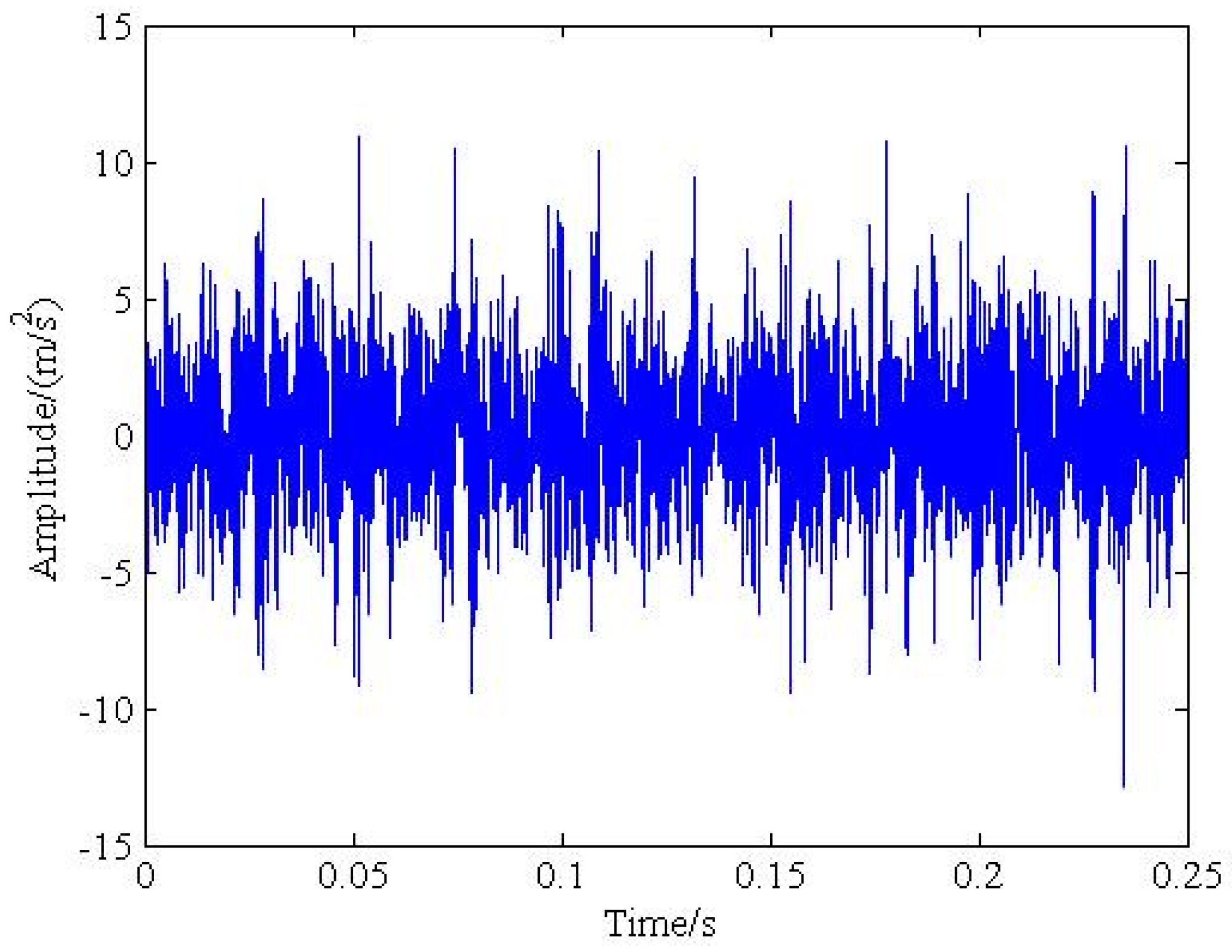
Figure 4 shows the time-domain diagram of the measured vibration signals, which indicates that the outer race fault feature is hardly detected by time-domain characteristic and it is necessary to analyze using the advanced analysis method. Additionally, the noisy component has an impact on the identification of bearing fault characteristic frequency. In order to show the detailed information on the signal with noise, the time scale is selected from zero to 0.25 s.
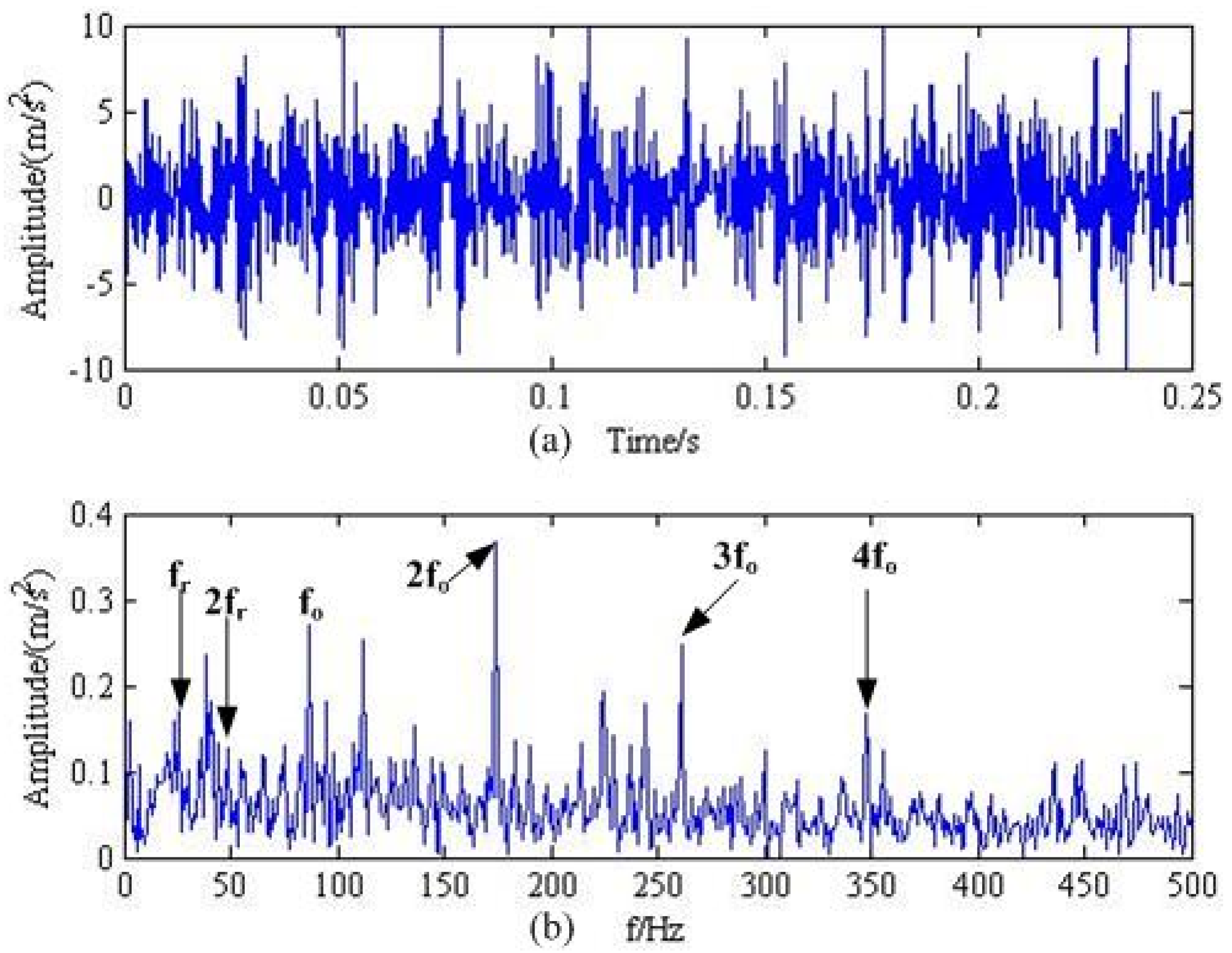
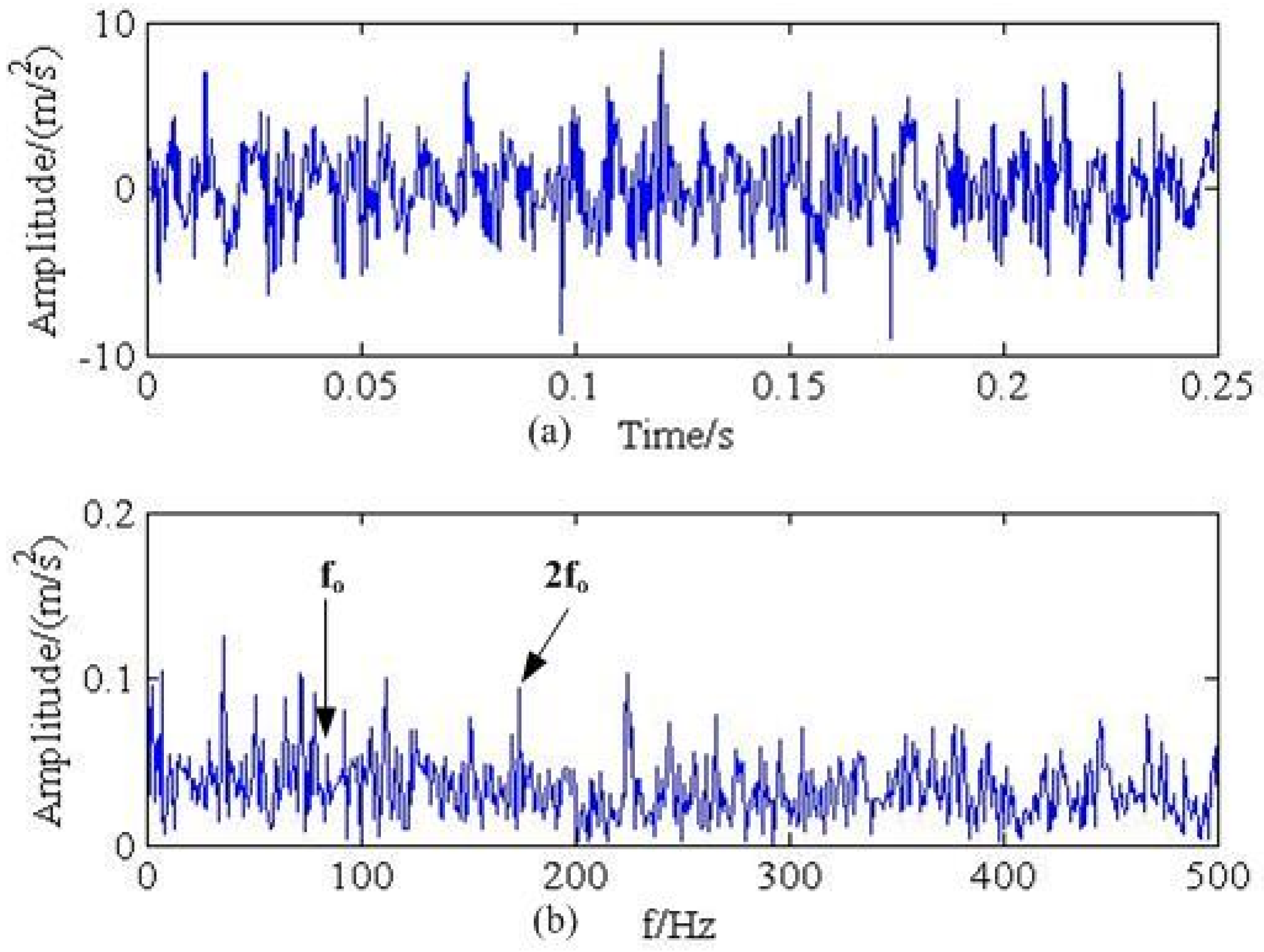
In order to compare the effect of different denoising methods for identifying mechanical failure characteristic frequency, the wavelet analysis and the proposed second-order TV methods with non-convex penalty function were used to analyze the measured bearing fault signal. After using the regularization parameter selection method, we can obtain λ = 1.1 . The results are shown in Figure 5 and Figure 6, respectively. The denoising result by the proposed method in time-domain was shown in Figure 5a. Meanwhile, directly frequency spectrum analysis was carried out and plotted in Figure 5b. From Figure 5b, it can be seen that the proposed method can clearly detect outer race fault frequency 87 Hz ( f o ), second harmonic frequency 175 Hz ( 2 f o ), the third harmonic frequency 262 Hz ( 3 f o ), and quadruplicated frequency 349 Hz ( 4 f o ). Additionally, the rotation frequency f r and its second harmonic frequency 2 f r can be inspected. The conclusion can be made that there is an outer race fault on the bearing test rig, which is consistent with the actual situation. The typical wavelet denoising method with previous parameter settings was also used to analyze the data and the results are shown in Figure 6. Similarly, the time-domain graph and frequency-domain graph were plotted in Figure 6a,b, respectively. Since the amplitude of fault frequency of the outer race is smaller than the others, it can be hardly identified by the wavelet denoising method. Thus, the result demonstrated that the proposed improved total variation method has greater superiority in signal denoising.

5. Verification by Industrial Bearing Fault Signal

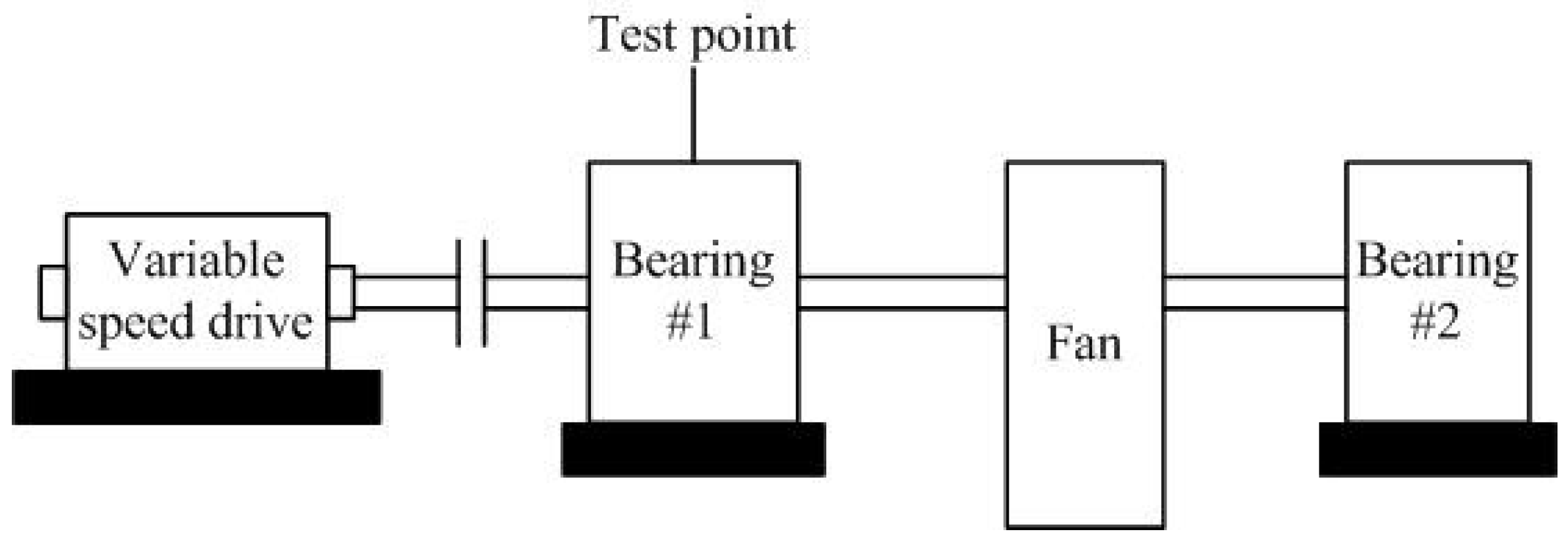
To further verify the proposed improved total variation denoising method in the industrial field equipment fault diagnosis, the bearing signal of an exhaust fan in metallurgical industry was analyzed in this paper. The exhaust fan is mainly used in iron-making processing, which is one of the important pieces of equipment in the plant. The equipment structure diagram and bearing under test position is shown in Figure 7.
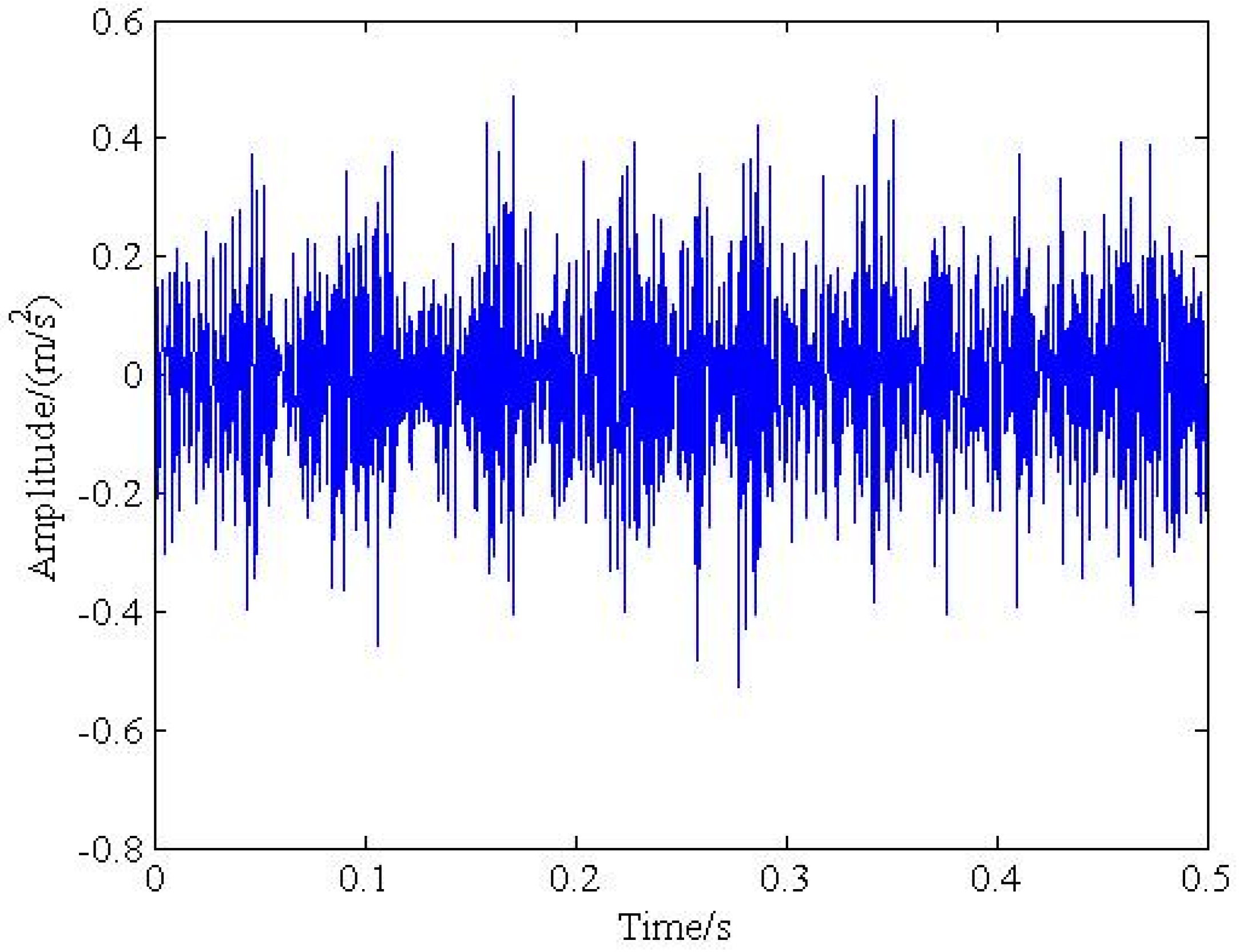
In order to obtain the running state of the fan, the US Emerson CSI2130 vibration acquisition equipment is used to test the vertical position of the bearing in Figure 7. The type of tested roller bearing is SKF22230. Equipment operating parameters, data acquisition parameters and bearing fault frequencies are shown in Table 3. The sampling rate is 2560 Hz, the rotation frequency is f r = 16.5 Hz and the fault frequency of the outer race is f o = 135.3 Hz, respectively. The measured vibration signal of an exhaust fan in time-domain is plotted in Figure 8. The time scale is selected from zero to 0.5 s so as to display the the detailed information on the measured signal.
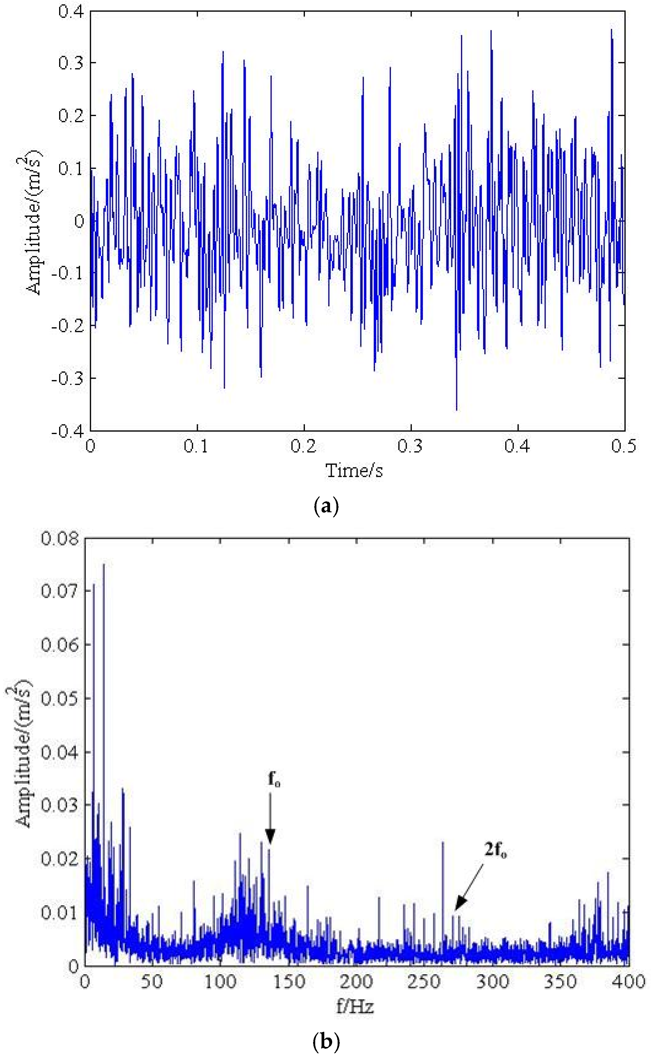
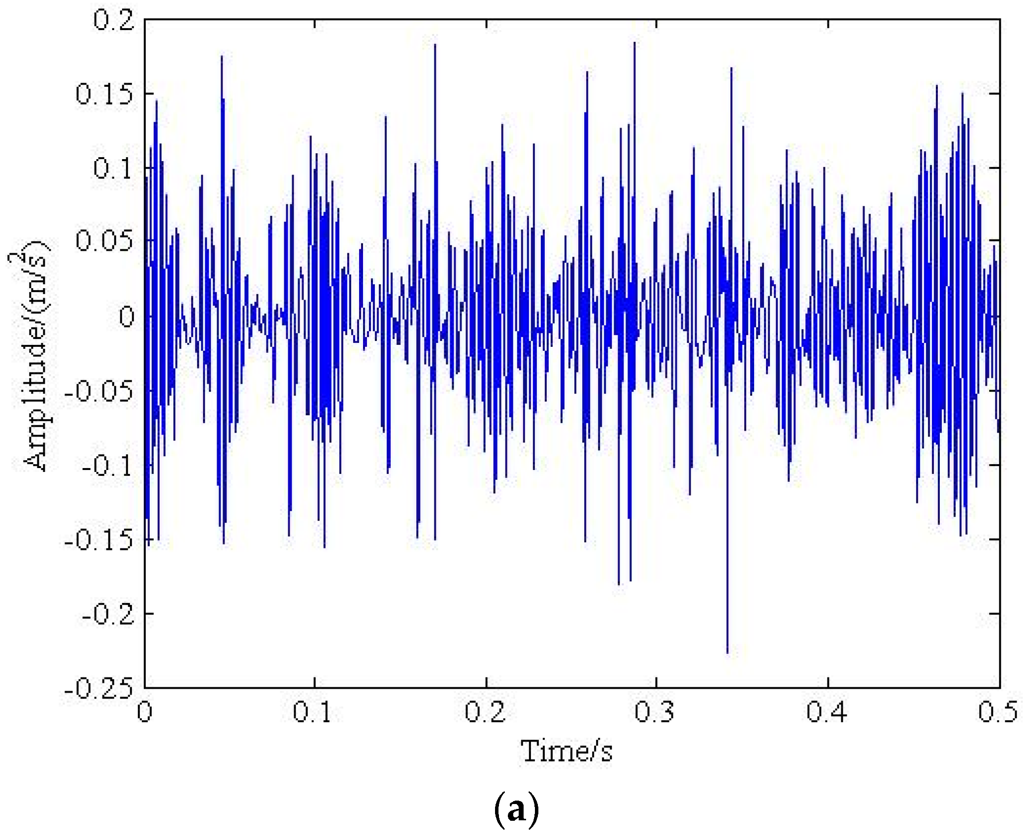
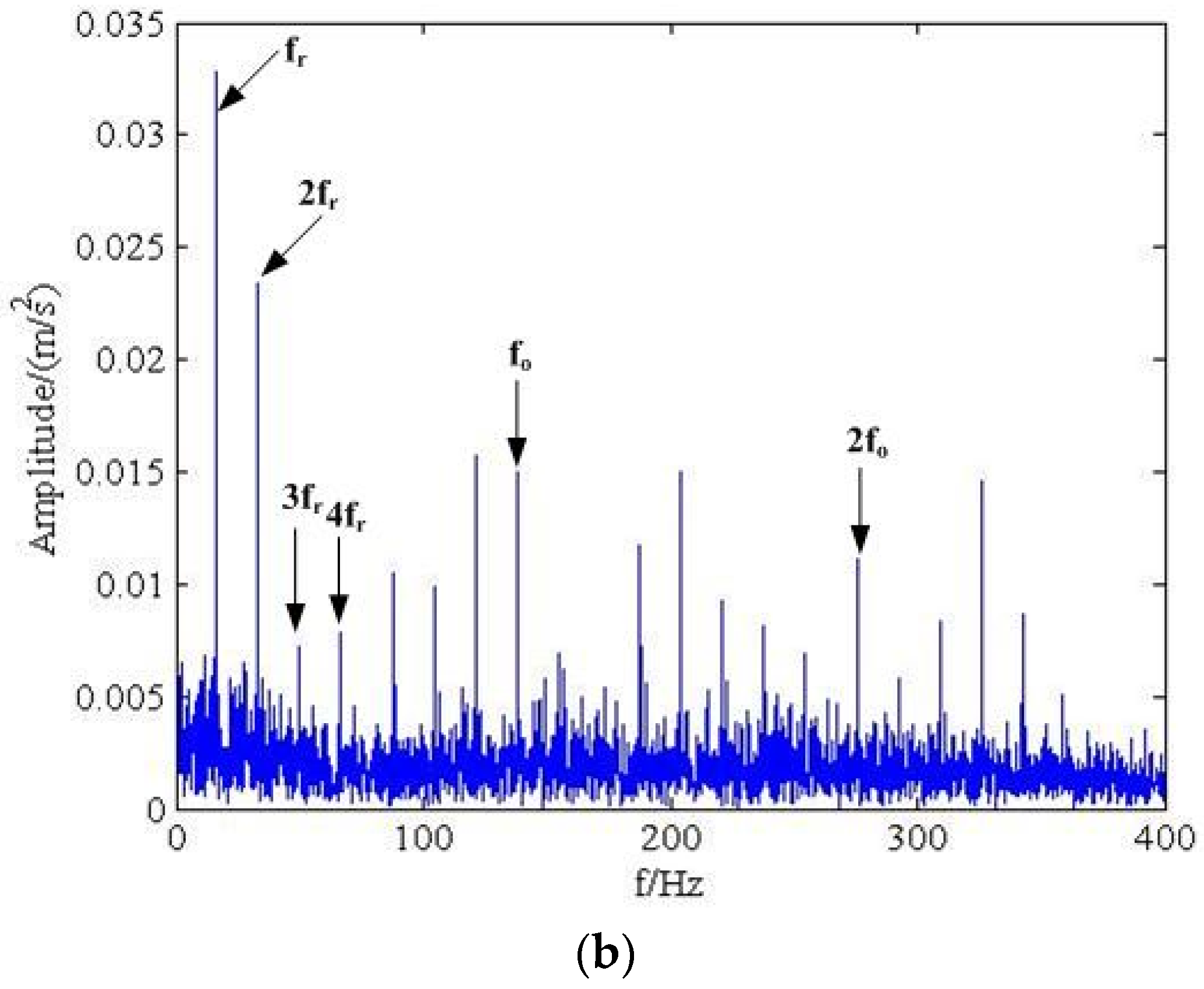
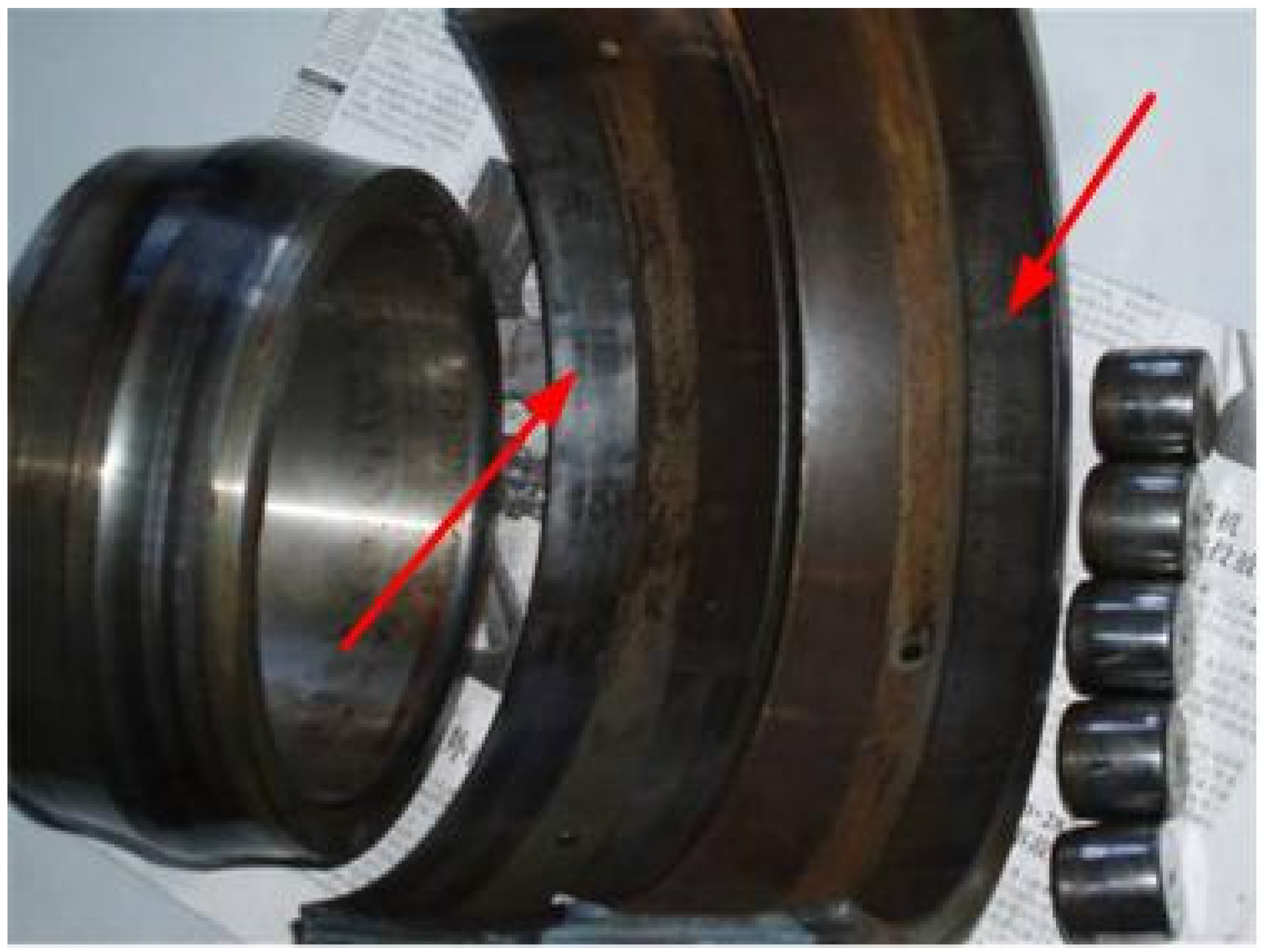
Fan vibration signal is processed by the proposed improved total variation denoising method and typical wavelet denoising method. The results are shown in Figure 9 and Figure 10, respectively. In Figure 9, only the outer race fault frequency and its second harmonic frequency can be detected by the wavelet method, which are not obvious. However, the proposed improved total variation denoising method can find the 16.59 Hz ( f r ) rotating frequency, second harmonic frequency 33.13 Hz ( 2 f r ), third harmonic frequency 49.69 Hz ( 3 f r ), the outer ring fault characteristic frequency 138 Hz ( f o ) and its second harmonic frequency 276 Hz ( 2 f o ), shown in Figure 10. Therefore, we can identify the fault of outer race in tested rolling bearing. Then, the first bearing is maintained and disintegrated later. A large area pitting on the outer ring is detected and the side surface of the radial has a serious scratch. The result of the disintegrated bearing is signalled by the red arrow in Figure 11, which is consistent with the results of the vibration testing and signal analysis. Thus, it is illustrated that the proposed approach can be successfully used in industrial bearing fault signal processing.

6. Conclusions

The main research work is described in the following three aspects: (1) The second-order total variation denoising method based on non-convex regularization was proposed, which aimed to guarantee the optimization problem was strictly convex and to improve the sparsity of the result. Besides, it can avoid the problem of staircase artifacts; (2) The composite indicator of permutation entropy and cross correlation coefficient were utilized in this paper, which performs well in ensuring greater signal-to-noise ratio and avoiding the detailed information loss caused by excessive denoising; (3) The second-order total variation denoising method with non-convex penalty function was applied to mechanical fault signal feature extraction. The results of numerical simulation signal, bearing fault signal in test rig and the exhaust fan in metallurgical industry, demonstrated that the proposed method has better denoising performance than the traditional TV method using first-order difference operator and wavelet denoising method.

Acknowledgments

This work was supported by the National Natural Science Foundation of China (Nos. 51475339, 51405353, 51375354), the Natural Science Foundation of Hubei province under Grants No. 2016CFA042, the Key Laboratory of Metallurgical Equipment and Control of Education Ministry, Wuhan University of Science and Technology (No. 2015B11) and the State Key Laboratory of Refractories and Metallurgy, Wuhan University of Science and Technology (No. ZR201603).

Author Contributions

Cancan Yi, Yong Lv, Zhang Dang and Han Xiao conceived and designed the experiments; Cancan Yi and Zhang Dang performed the experiments; Cancan Yi and Yong Lv analyzed the data; Cancan Yi and Han Xiao contributed reagents/materials/analysis tools; Cancan Yi and Han Xiao wrote the paper.

Conflicts of Interest

The authors declare no conflict of interest.

References

  1. Luo, H.; Lu, W.; Wang, Y.; Wang, L.; Zhao, X. A novel approach for analog fault diagnosis based on stochastic signal analysis and improved GHMM. Measurement 2016, 81, 26–35. [Google Scholar] [CrossRef]
  2. Dolenc, B.; Boškoski, P.; Juričić, Đ. Distributed bearing fault diagnosis based on vibration analysis. Mech. Syst. Signal Process. 2016, 66, 521–532. [Google Scholar] [CrossRef]
  3. Luo, S.; Cheng, J.; Zeng, M.; Yang, Y. An intelligent fault diagnosis model for rotating machinery based on multi-scale higher order singular spectrum analysis and GA-VPMCD. Measurement 2016, 87, 38–50. [Google Scholar] [CrossRef]
  4. Feng, Z.; Qin, S.; Liang, M. Time-frequency analysis based on Vold-Kalman filter and higher order energy separation for fault diagnosis of wind turbine planetary gearbox under nonstationary conditions. Renew. Energy 2016, 85, 45–56. [Google Scholar] [CrossRef]
  5. Wang, Y.; Xiang, J.; Markert, R.; Liang, M. Spectral kurtosis for fault detection, diagnosis and prognostics of rotating machines: A review with applications. Mech. Syst. Signal Process. 2016, 66, 679–698. [Google Scholar] [CrossRef]
  6. An, X.; Jiang, D.; Liu, C.; Zhao, M. Wind farm power prediction based on wavelet decomposition and chaotic time series. Expert Syst. Appl. 2011, 38, 11280–11285. [Google Scholar] [CrossRef]
  7. Qu, J.; Zhang, Z.; Gong, T. A novel intelligent method for mechanical fault diagnosis based on dual-tree complex wavelet packet transform and multiple classifier fusion. Neurocomputing 2016, 171, 837–853. [Google Scholar] [CrossRef]
  8. Huang, N.E.; Shen, Z.; Long, S.R.; Wu, M.C.; Shih, H.H.; Zheng, Q.; Yen, N.; Tung, C.C.; Liu, H.H. The empirical mode decomposition and the Hilbert spectrum for nonlinear and non-stationary time series analysis. Proc. R. Soc. Lond. A Math. Phys. Eng. Sci. 1998, 454, 903–995. [Google Scholar] [CrossRef]
  9. Fan, G.; Peng, L.; Hong, W.; Sun, F. Electric load forecasting by the SVR model with differential empirical mode decomposition and auto regression. Neurocomputing 2016, 173, 958–970. [Google Scholar] [CrossRef]
  10. Hassan, A.R.; Bhuiyan, M.I.H. Computer-aided sleep staging using complete ensemble empirical mode decomposition with adaptive noise and bootstrap aggregating. Biomed. Signal Process. Control 2016, 24, 1–10. [Google Scholar] [CrossRef]
  11. Yan, X.G.; Edwards, C. Nonlinear robust fault reconstruction and estimation using a sliding mode observer. Automatica 2007, 43, 1605–1614. [Google Scholar] [CrossRef]
  12. Yan, X.G.; Edwards, C. Fault estimation for single output nonlinear systems using an adaptive sliding mode estimator. IET Control Theory Appl. 2008, 2, 841–850. [Google Scholar] [CrossRef]
  13. Condat, L. A Direct Algorithm for 1-D Total Variation Denoising. IEEE Signal Process. Lett. 2013, 20, 1054–1057. [Google Scholar] [CrossRef] [Green Version]
  14. Couprie, C.; Grady, L.; Najman, L.; Pesquet, J.-C.; Talbot, H. Dual constrained TV-based regularization on graphs. SIAM J. Imaging Sci. 2013, 6, 1246–1273. [Google Scholar] [CrossRef] [Green Version]
  15. Chen, G.; Zhang, J.; Li, D.; Chen, H. Robust Kronecker product video denoising based on fractional-order total variation model. Signal Process. 2016, 119, 1–20. [Google Scholar] [CrossRef]
  16. Mila, N.; Ng, M.K.; Chi-Pan, T. Fast nonconvex nonsmooth minimization methods for image restoration and reconstruction. IEEE Trans. Image Process. 2010, 19, 3073–3088. [Google Scholar]
  17. Selesnick, I.W.; Parekh, A.; Bayram, I. Convex 1-D Total Variation Denoising with Non-convex Regularization. IEEE Signal Process. Lett. 2015, 22, 141–144. [Google Scholar] [CrossRef]
  18. He, W.; Yi, C.; Li, Y.; Xiao, H. Research on Mechanical Fault Diagnosis Scheme Based on Improved Wavelet Total Variation Denoising. Shock Vib. 2016, 2016, 3151802. [Google Scholar] [CrossRef]
  19. Liu, P.; Xiao, L. Efficient multiplicative noise removal method using isotropic second order total variation. Comput. Math. Appl. 2015, 70, 2029–2048. [Google Scholar] [CrossRef]
  20. Bergmann, R.; Weinmann, A. A Second-Order TV-Type Approach for Inpainting and Denoising Higher Dimensional Combined Cyclic and Vector Space Data. J. Math. Imaging Vis. 2016, 55, 401–427. [Google Scholar] [CrossRef]
  21. Christoph, B.; Bernd, P. Permutation entropy: A natural complexity measure for time series. Phys. Rev. Lett. 2002, 88, 174102. [Google Scholar]
  22. Shi, W.; Shang, P.; Lin, A. The coupling analysis of stock market indices based on cross-permutation entropy. Nonlinear Dyn. 2015, 79, 2439–2447. [Google Scholar] [CrossRef]
  23. Li, Y.; Xu, M.; Wei, Y.; Wang, W. A new rolling bearing fault diagnosis method based on multiscale permutation entropy and improved support vector machine based binary tree. Measurement 2016, 77, 80–94. [Google Scholar] [CrossRef]
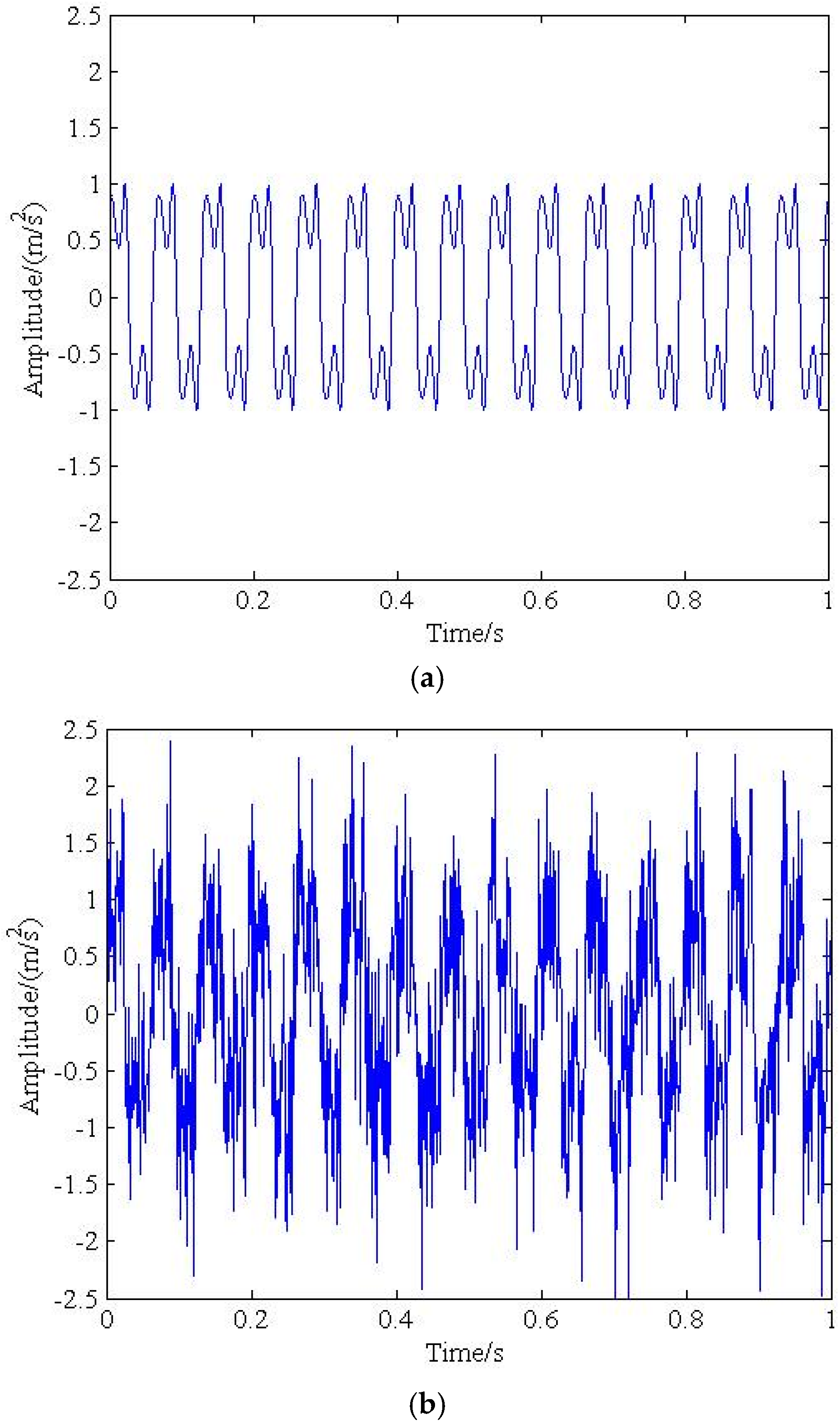
Figure 1. The clean signal and noisy signal with δ = 0.5 . (a) The time response of the clean signal; (b) The time response of the noisy signal.
Applsci 06 00403 g001
Figure 2. Comparison of the different denoising methods. (a) Simulation results of TV denoising; (b) Simulation results of wavelet transforms denoising; (c) The results provided by the proposed method.
Applsci 06 00403 g002
Figure 3. Bearing test rig.
Applsci 06 00403 g003
Figure 4. The measured vibration signal of bearing test rig in time-domain.
Applsci 06 00403 g004
Figure 5. Results obtained by the proposed method, (a) Reconstructed signal in time-domain by the proposed method; (b) Reconstructed signal in frequency-domain by the proposed method.
Applsci 06 00403 g005
Figure 6. Results obtained by typical wavelet denoising, (a) Reconstructed signal in time-domain by wavelet; (b) Reconstructed signal in frequency-domain by wavelet.
Applsci 06 00403 g006
Figure 7. The structure diagram of the fan.
Applsci 06 00403 g007
Figure 8. The measured vibration signal of an exhaust fan in time-domain.
Applsci 06 00403 g008
Figure 9. Result provided by wavelet denoising. (a) Result of wavelet denoising in time-domain; (b) Result of wavelet denoising in frequency-domain.
Applsci 06 00403 g009
Figure 10. Result obtained by the proposed method. (a) Result of proposed method in time-domain; (b) Result of proposed method in frequency-domain.
Applsci 06 00403 g010aApplsci 06 00403 g010b
Figure 11. Picture of bearing components after test (outer race defect in bearing).
Applsci 06 00403 g011
Table 1. The performance of different denoising methods. SNR: signal-to-noise ratio; TV: total variation.
The Variance of NoiseThe SNR after Denoising by Different Methods
The Proposed MethodTV DenoisingWavelet Denoising
0.118.669.0615.59
0.216.528.4112.44
0.315.157.0711.57
0.412.134.6910.28
0.511.313.319.20
0.610.282.178.31
Table 2. The experiment parameter and failure frequency of bearing.
Rotation Speed r/minRotation Frequency/HzSampling Rate/HzSampling Time/sOuter Fault/Hz
145024.1716384187.01
Table 3. The experiment parameter and failure frequency of fan.
Rotation Speed r/minRotation Frequency/HzSampling Rate/HzSampling Time/sOuter Fault/Hz
99316.525606.39135.3