Article

Decentralized Integral-Based Event-Triggered Stabilization for Linear Plant with Actuator Saturation and Output Feedback

1
Institute of Mathematics and Statistics, Chifeng University, ChiFeng, Inner Mongolia 024000, China
2
The Seventh Research Division, School of Automation Science and Electrical Engineering, Beihang University, Beijing 100191, China
*
Author to whom correspondence should be addressed.
Appl. Sci. 2017, 7(1), 11; https://doi.org/10.3390/app7010011
Submission received: 28 October 2016 / Revised: 9 December 2016 / Accepted: 16 December 2016 / Published: 22 December 2016

Abstract

:
This paper studies the integral-based event-triggered asymptotic stabilization for a continuous-time linear plant. Both actuator saturation and observer-based output feedback are considered. The sensors and actuators are implemented in a decentralized manner and a type of Zeno-free decentralized integral-based event condition is designed to guarantee the asymptotic stability of the closed-loop systems. The positive lower bound of inter-event times is guaranteed by enforcing the event conditions not to be triggered until some fixed intervals. A linear optimization problem is introduced to find the largest stability region. Moreover, the co-design of the parameters in event conditions and the controller gain matrices is proposed in terms of linear matrix inequalities. Finally, two numerical examples are given to illustrate the efficiency and the feasibility of the proposed results.

1. Introduction

In the last decade, event-triggered control attracts more and more attention due to the advantages of reducing the number of control task executions and the cost of communication resources. In this control strategy, the control task execution is decided by an event instead of a certain fixed period of time. The latter is known as periodic sampling or time-triggered control [1]. The event is generated by the designed event condition, which is a state-related criterion. Therefore, event-triggered control can make the control tasks executed when necessary as the way a human performs [2]. In [3,4,5], the authors studied the state-feedback event-triggered control from an input-to-state stable point of view and proposed several types of event conditions to guarantee the asymptotic stability of the closed-loop systems. It is noted that the aforementioned works assumed that all the states are available to the controller, but this assumption is excessive and inappropriate in some situations. Therefore, [6,7] studied the dynamic output feedback event-triggered control for certain and uncertain linear systems. Furthermore, the quantization effect on the dynamic output-feedback event-triggered control was considered in [8]. Ref. [9] applied a cyclic small-gain approach to analyze the event-triggered control systems with partial states and output feedback. The centralized or decentralized event-triggered control in networks was studied in [10,11,12]. The latest survey on event-triggered control can be found in [13,14]. To further improve the sampling performance, such as enlarging the average inter-event time or equivalently decreasing the sampling numbers within a fixed time interval, a novel integral-based event-triggered control scheme was recently proposed in [15,16]. Literally, the integral-based event-triggered control utilizes the integrals of the measurement signals to construct the event conditions. By this means, this control scheme can allow the Lyapunov function to be non-decrescent between two consecutive triggering instants. Consequently, the integral-based event-triggered control can be proved to yield better sampling performance than the scheme in [3].
Additionally, actuator saturation is a ubiquitous phenomenon in practical control systems due to the limitation of the facilities. It has been observed that the actuator saturation has a remarkable effect on the performance of the control systems (see [17] and the references therein). There are few literatures studied event-triggered control with saturated inputs. In [18] and its follow-up work [19], the authors studied event-triggered output feedback control for linear systems with actuator saturation, where the practical stability is guaranteed. Then, they applied the anti-windup approach to improve the performance of the systems. For a discrete-time linear plant, the event-triggered control subject to actuator saturation was studied in [20]. Recently, Ref. [21] studied the event-triggered asymptotic stabilization of a continuous-time plant with saturated inputs in both static state feedback and dynamic output feedback configurations. A kind of centralized relative event condition is employed in [21], which is also applied in [3,22].
In this paper, we study the event-triggered asymptotic stabilization of a continuous-time linear plant with output feedbacks and saturated inputs. The contributions of this paper are described as follows. First, the decentralized event-triggered control with actuator saturation and output feedback is considered. In some situations, such as implementations over Wireless Sensor Actuator Networks, the sensors and actuators are grouped physically into several nodes and each of them has no access to the measurements of the others (see, e.g., [23,24,25]). As a result, the event condition of each node can only utilize its own measurement, and, hence, the event-triggered control in this paper is executed in a decentralized manner. Second, a type of Zeno-free integral-based event condition is proposed to ensure the asymptotic stability. By enforcing the decentralized event conditions to not be triggered until some fixed intervals, the positive lower bound of inter-event time is guaranteed. Then, beyond these intervals, the integral-based event conditions are used to improve the sampling performance. Compared to [25], a different mathematical technique (which is based on the Cauchy–Schwarz inequality) is employed to design these intervals analytically from the integral-based event conditions. To the best of our knowledge, the existing contributions on integral-based event-triggered control (see, e.g., [15,16,26]) did not involve the decentralised output feedback configuration and/or the saturated input signals.
The remainder of this paper is organised as follows. After the necessary notation is introduced in Section 3, a decentralized integral-based event-triggered output feedback saturated control system is formulated in Section 2. The main results of this paper are included in Section 4. Two numerical examples are provided to illustrate the efficiency and the feasibility of the proposed results in Section 5. Finally, the conclusions of this paper are drawn in Section 6.

2. Preliminaries

The set of real numbers is denoted by R . The set of nonnegative integers is denoted by N 0 . The transpose of a matrix A R n × m is denoted by A T R m × n . s represents the absolute value of a scalar s. The Euclidian norm of a vector x R n is denoted by x , and let x denote its infinity norm, i.e., x = max i = 1 , , n x i . t r ( A ) represents the trace of a matrix A and its induced two-norm is denoted by A : = max λ { A T A } , where λ { A T A } denotes all of the eigenvalues of A T A . An asterisk ( ) in the matrix is used to present a symmetry block. For a symmetric matrix P R n × n , P > 0 ( P 0 ) denotes that it is positive (semi-)definite, and, similarly, P < 0 ( P 0 ) means that it is a negative (semi-)definite matrix. Let I m R m × m ( 0 m × n R m × n ) represent the identity (zero) matrix, and, for brevity, we sometimes omit the subscript of I m ( 0 m × n ) if there is no confusion from the contexts. The saturation function for a scalar s with upper bound c, s a t c ( · ) , is defined as s a t c ( s ) = sign ( s ) min { c , s } , where sign ( · ) denotes the sign function. In addition, the vector saturation function is defined as s a t c ( x ) = ( s a t c ( x 1 ) , , s a t c ( x n ) ) with x = ( x 1 , , x 2 ) T . For a group of points, p 1 , p 2 , , p l , the convex hull of these points is defined as c o { p k , k = 1 , , l } = { k = 1 l α k p k | k = 1 l α k = 1 , α k 0 } .
To deal with the saturation property, we introduce some lemmas for later use. Define D as the set of m-demision diagonal matrices whose diagonal elements are either 1 or 0. Obviously, there are 2 m elements in D . Label all elements in D as D j + , j M : = { 1 , 2 , , 2 m } and denote D j = I D j + . For a positive definite matrix P R n × n , define an ellipsoid Γ ( P ) by
Γ ( P ) : = { x R | x T P x 1 } .
For a given matrix H R m × n , denote the j-th row of H as h j . Then, we define
L ( H ) : = { x R n | h j x 1 , j 1 , , 2 } .
With these definitions, we introduce the following lemmas.
Lemma 1.
[27] For a given u , v R m with u = ( u 1 , u 2 , , u m ) T and v = ( v 1 , v 2 , , v m ) T , suppose v 1 . Then,
s a t ( u ) c o { D j + u + D j v | j M } .
Lemma 2.
[28] For a given Γ ( P ) and L ( H ) , if
1 h j P 0 , j { 1 , , m } ,
where h j denotes the j th row of H, then Γ ( P ) L ( H ) .

3. Problem Formulation

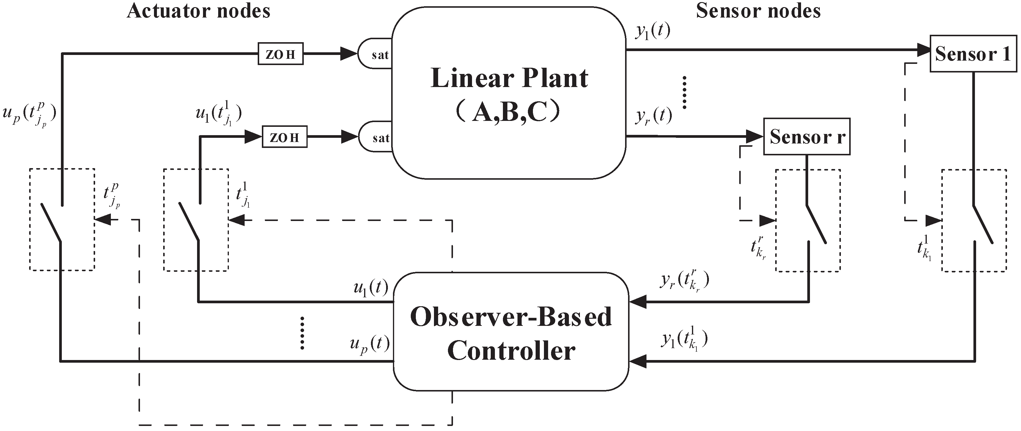
For clarity, the decentralized event-triggered output feedback saturated control system is illustrated in Figure 1 at first, and the specific details will be given later.
Consider the following linear time-invariant plant with saturated input
x ˙ = A x + B s a t ( u ¯ ) , y = C x ,
where x R n , u ¯ R m , and y R q are, respectively, the state vector, the control input, and the output. A , B , C are constant matrices of appropriate dimensions. ( A , B ) is supposed to be controllable, and ( A , C ) is supposed to be observable. For briefness, we assume that in the following analysis, the upper bound for the saturation function is c = 1 and the subscript c is dropped. As shown in Figure 1, both control signal u ( t ) and output y ( t ) are implemented in a decentralized manner. Hence, they are, respectively, partitioned into p actuator nodes and r sensor nodes, i.e., u = ( u 1 T , , u p T ) T and y = ( y 1 T , , y r T ) T , where u s R m s , s { 1 , 2 , , p } and y l R q l , l { 1 , 2 , , r } . m s ( q l ) denotes the dimension of the sth (lth) actuator (sensor) node and satisfies σ s = 1 p m s = m ( σ l = 1 r q l = q ). To identify the nodes, we introduce the matrices Π u s R m s × m and Π y l R q l × q defined as
Π u s = ( 0 m s × m 1 , , 0 m s × m s 1 , I m s , 0 m s × m s + 1 , , 0 m s × m p ) , Π y l = ( 0 q l × q 1 , , 0 q l × q l 1 , I q l , 0 q l × q l + 1 , 0 q l × q r ) .
Thus, u s = Π u s u and y l = Π y l y . Because of the communication constraints, either between sensors and observer, or between observer and actuators, the information cannot be transmitted continuously.
Denote y l ( t k l l ) , l = 1 , , r , k l N 0 as the latest sampled value at the l t h sensor node, which is available for the observer-based controller to calculate the control signal. u s ( t j s s ) , s = 1 , , p , j s N 0 is the latest sampled actuator signal applied to the system. The triggering instants t k 1 1 , , t k r r , t j 1 1 , , t j p p are decided by the designed event condition. It is worth noting that different sensor nodes and different actuator nodes are sampled asynchronously. Thus, at time t, the latest available output y ¯ ( t ) is
y ¯ ( t ) = ( y 1 T ( t k 1 1 ) , , y r T ( t k r r ) ) T ,
and the input u ¯ ( t ) is
u ¯ ( t ) = ( u 1 T ( t j 1 1 ) , , u p T ( t j p p ) ) T .
Moreover, it is supposed that the first triggering instants of all the nodes are the initial instant, i.e., t 0 l = t 0 s : = t 0 , for l = 1 , , r and s = 1 , , p .
Therefore, the observer-based controller can be described as
x ^ ˙ = A x ^ + L ( y ¯ C x ^ ) + B s a t ( u ¯ ) , u = K x ^ ,
where x ^ is the state of observer. The matrices K and 
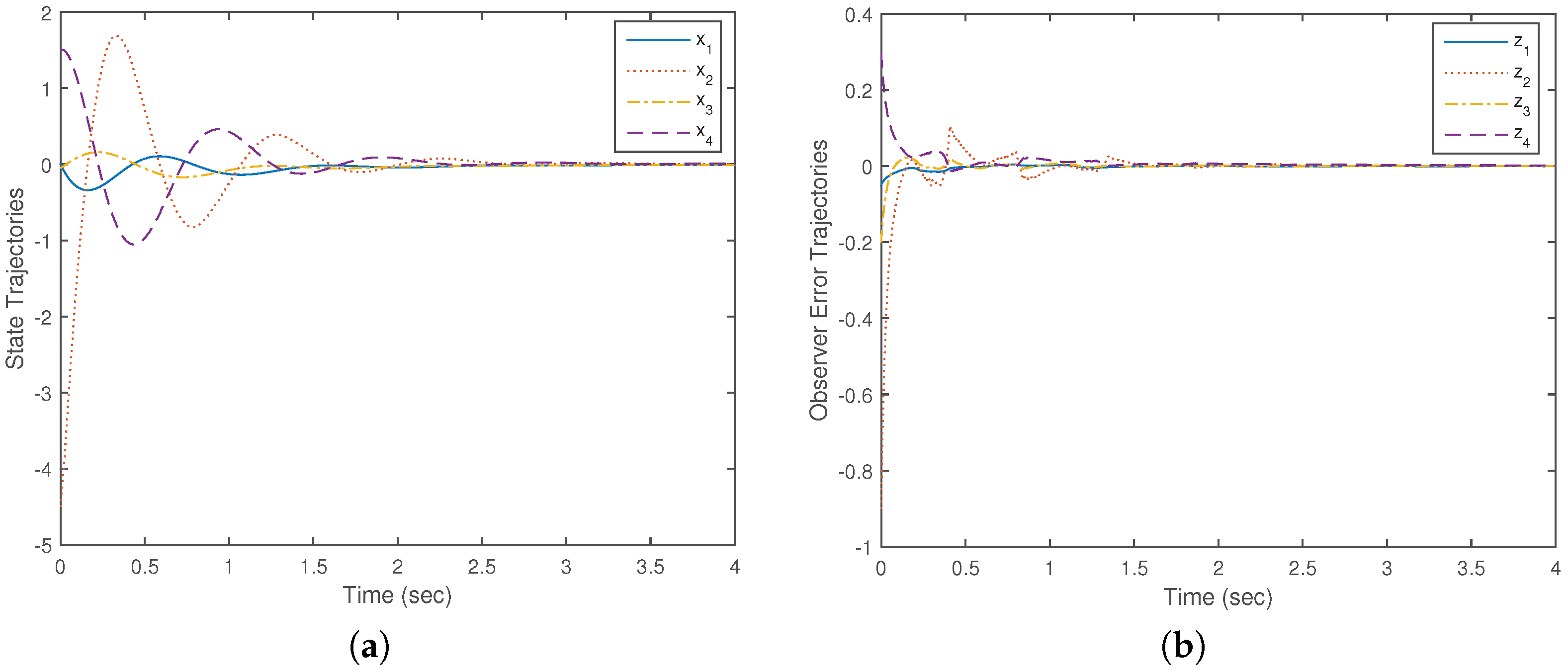
L are gain matrices to be designed. Denote the observer error by z = x ^ x . Then, its dynamic becomes
z ˙ = x ^ ˙ x ˙ = A z + L ( y ¯ C x ^ ) .
Define the sampling error as E = ( e u T , e y T ) T , where e u = u ¯ u and e y = y ¯ y . Then, we introduce the following decentralized integral-based event condition for each sensor/actuator node:
t j s + 1 s = inf t { t t j s s + τ u s | t j s s t e u s 2 d ω > σ u s t j s s t u s 2 d ω } , s = 1 , , p ,
t k l + 1 l = inf t { t t k l l + τ y l | t k l l t e y l 2 d ω > σ y l t k l l t y l 2 d ω } , l = 1 , , r ,
where σ y l , τ y l , σ u s and τ u s are positive constants to be designed.
Remark 1.
In Ref. [15], the centralised state feedback was considered, and it was proved that the positive minimum inter-event time can be ensured automatically by the integral part of the event condition (4). According to [22,24], however, it is difficult to avoid Zeno behaviors in both the decentralised and the output feedback configurations. Hence, we introduce the positive constants τ y l and τ u s to guarantee the positive minimum inter-event time. For example, the minimum inter-event time of u 1 cannot obviously be less than τ u 1 .
From Label (1) and Label (3), the closed-loop system becomes
x ˙ = A x + B s a t ( K x + K z + e u ) , z ˙ = ( A L C ) z + L e y .
Therefore, the main interest of this paper is to design the gain matrices K, L and the decentralized integral-based event condition (4) such that the closed-loop system (5) is asymptotically stable. To this end, we first assume the gain matrices to be given and provide results for designing the event condition. Then, we consider the co-design problem of the gain matrices and the event condition.

4. Theoretical Results

In this section, we provide the main results of this paper. First, we propose a method based on linear matrix inequality (LMI) to design the event condition (4) in the case that the gain matrices are supposed to be given. Then, we will study the synthesis of the gain matrices. Let the argument variable be X c = ( x T , z T ) T . Motivated by [21], we initially use Lemma 1 to deal with the saturation nonlinearity, which shows that if H X c 1 for a matrix H = ( H 1 , H 2 ) , H i R m × n , i = 1 , 2 , then
B s a t ( K x + K z + e u ) c o { B D j + ( K x + K z + e u ) + B D j ( H 1 x + H 2 z ) , j M } .
Now, consider the state X c in the set { X c R 2 n | H X c 1 } . At this moment, the closed-loop system (5) is translated into the following form:
x ˙ c o { ( A + B D j + K + B D j H 1 ) x + ( B D j + K + B D j H 2 ) z + B D j + e u , j M } , z ˙ = ( A L C ) z + L e y .
Then, we study the stability of this differential inclusion. Let V = x T P 1 x + z T P 2 z with P 1 , P 2 being n-dimension positive definite matrices. The derivative of V along the trajectories of Label (6) is
V ˙ c o { 2 x T P 1 A c x + 2 x T P 1 B D j + K z + 2 x T P 1 B D j H 2 z + 2 x T P 1 B D j + e u + 2 z T P 2 ( A L C ) z + 2 z T P 2 L e y , j M } ,
with A c = A + B D j + K + B D j H 1 . From the fact 2 x T P 1 B D j + K z ε 1 z T z + 1 ε 1 x T P 1 B D j + K ( P 1 B D j + K ) T x for any ε 1 > 0 ,
V ˙ c o { x T ( 2 P 1 A c + 1 ε 1 P 1 B D j + K ( P 1 B D j + K ) T ) x + 2 x T P 1 B D j H 2 z + 2 x T P 1 B D j + e u + z T ( 2 P 2 ( A L C ) + ε 1 I ) z + 2 z T P 2 L e y , j M } .
According to Label (7), a sufficient condition for V ˙ < 0 is
X c T φ 11 P 1 B D j H 2 φ 22 X c + 2 X c T P 1 B D j + 0 0 P 2 L E < 0 , j M ,
where φ 11 = P 1 A c + A c T P 1 + 1 ε 1 P 1 B D j + K ( P 1 B D j + K ) T and φ 22 = P 2 ( A L C ) + ( A L C ) T P 2 + ε 1 I . Due to the fact that, for any ε 2 > 0 ,
2 X c T P 1 B D j + 0 0 P 2 L E ε 2 E T E + 1 ε 2 X c T P 1 B D j + 0 0 P 2 L ( P 1 B D j + ) T 0 0 L T P 2 T X c ,
if the following matrix inequality holds for some positive scalar ρ 0 ,
φ 11 + 1 ε 2 ( P 1 B D j + ) ( P 1 B D j + ) T + ε 2 ρ 0 2 I P 1 B D j H 2 φ 22 + ε 2 ρ 0 2 I + 1 ε 2 P 2 L ( P 2 L ) T < 0 , j M ,
then V ˙ < ε 2 ( ρ 0 2 X c T X c + E T E ) .
By a Schur complement, Label (9) is equivalent to
ψ 11 P 1 B D j H 2 P 1 B D j + 0 P 1 B D j + K ψ 22 0 P 2 L 0 ε 2 I 0 0 ε 2 I 0 ε 1 I < 0 , j M ,
where ψ 11 = P 1 A c + A c T P 1 + ε 2 ρ 0 2 I , ψ 22 = P 2 ( A L C ) + ( A L C ) T P 2 + ( ε 1 + ε 2 ρ 0 2 ) I and A c = A + B D j + K + B D j H 1 . Hence, at this moment, V ˙ < ε 2 ( ρ 0 2 X c T X c + E T E ) . If the event condition (4) ensures t 0 t E T E d s θ ρ 0 2 t 0 t X c T X c d ω with θ ( 0 , 1 ) , then V ( t ) V ( 0 ) = t 0 t V ˙ d s < ( 1 θ ) ε 2 ρ 0 2 t 0 t X c T X c d ω 0 . As a result, if the ellipsoid Γ ( P 1 , P 2 ) : = { ( x T , z T ) T R 2 n | x T P 1 x + z T P 2 z 1 } satisfies
Γ ( P 1 , P 2 ) { X c R 2 n | H X c 1 } ,
then the set Γ ( P 1 , P 2 ) is an invariant set of the closed-loop system (5). Consequently, H X c 1 holds for all t t 0 . This means that the closed-loop system is stable. From Lemma 2, a sufficient condition for Label (11) is
1 h l + h l P 1 0 P 2 0 , l = 1 , , m ,
where h l + is the l th row of H 1 and h l is the l th row of H 2 . Then, we propose the following theorem to obtain the asymptotic stability.
Theorem 1.
Consider the closed-loop system (5). Suppose that there exist a group of solutions { P 1 > 0 , P 2 > 0 , ρ 0 2 > 0 , h l + , h l } to the LMIs (10) and (12) for some ε 1 , ε 2 > 0 . If the parameters in event condition (4) satisfy the following conditions:
1.
s = 1 p Π u s K ¯ 2 σ u s + l = 1 r Π y l C ¯ 2 σ y l < θ ρ 0 2 ,
2.
τ u s σ u s L 1 2 + θ ρ 0 2 L 2 2 , s = 1 , , p , and, τ y l σ y l L 1 2 + θ ρ 0 2 L 2 2 , l = 1 , , r ,
where θ ( 0 , 1 ) , L 1 = A ¯ + B ¯ K ¯ + B ¯ H , L 2 = B ¯ + L ¯ and the matrices are
A ¯ = A 0 0 A L C , B ¯ = B 0 , L ¯ = 0 L , K ¯ = K K , C ¯ = C 0 .
Then, for any initial state in the ellipsoid Γ ( P 1 , P 2 ) , the corresponding closed-loop system (5) is asymptotically stable.
Proof of Theorem 1.
If it is shown that the parameters in the theorem can guarantee t 0 t E T E d ω θ ρ 0 2 t 0 t X c T X c d ω for t [ t 0 , ) , then the stability can be proved directly according to the preceding analysis. To this end, we first consider the derivative of X c . From Label (6),
X ˙ c c o { ( A ¯ + B ¯ D j + K ¯ + B ¯ D j H ) X c + B ¯ D j + I 0 E + L ¯ 0 I E } , j M ,
which leads to
X ˙ c ( A ¯ + B ¯ K ¯ + B ¯ H ) X c + ( B ¯ + L ¯ ) E L 1 X c + L 2 E .
Similarly, one has
d d t e u s e ˙ u s Π u s K ¯ X ˙ c L 1 , u s X c + L 2 , u s E , s = 1 , , p ,
d d t e y l e ˙ y l Π y l C ¯ X ˙ c L 1 , y l X c + L 2 , y l E , l = 1 , , r ,
where L 1 , u s = Π u s K ¯ L 1 , L 2 , u s = Π u s K ¯ L 2 , L 1 , y l = Π y l C ¯ L 1 , and L 2 , y l = Π y l C ¯ L 2 .
Denote by { t k } k = 0 = s = 1 p { t j s s } l = 1 r { t k l l } the overall triggering instants. By definitions, there may exist more than one node being triggered for some t k . In addition, since there is no Zeno phenomenon, lim k t k = .
Initially, by contradiction, we prove the inequality t 0 t E T E d ω θ ρ 0 2 t 0 t X c T X c d ω for t [ t 0 , t 1 ) . If X c ( t 0 ) = 0 , the conclusion holds obviously. In the case X c ( t 0 ) 0 , assume the positive instant T 0 > t 0 (it allows being infinity) as the first time when t 0 T 0 E 2 d ω = θ ρ 0 2 t 0 T 0 X c 2 d ω . Such a T 0 exists because of E ( t 0 ) = 0 . If T 0 t 1 , the inequality holds. If T 0 < t 1 , t 0 t E T E d ω θ ρ 0 2 t 0 t X c T X c d ω for t [ t 0 , T 0 ] , and, at this point, it can be proved that for t [ t 0 , T 0 ] ,
t 0 t e u s 2 d ω σ u s Π u s K ¯ 2 t 0 t X c 2 d ω , t 0 t e y l 2 d ω σ y l Π y l C ¯ 2 t 0 t X c 2 d ω .
To illustrate Label (15), for example, we consider e u 1 .
First, in the case T 0 t 0 τ u 1 , Label (14a) implies that
e u 1 2 ( t 0 t L 1 , u 1 X c + L 2 , u 1 E d ω ) 2 2 ( t t 0 ) t 0 t L 1 , u 1 X c 2 + L 2 , u 1 E 2 d ω ,
where the last inequality employs the Cauchy–Schwarz inequality and the fact that ( a + b ) 2 < 2 a 2 + 2 b 2 . By integrating Label (16), one has
t 0 t e u 1 2 d ω ( t t 0 ) 2 t 0 t L 1 , u 1 X c 2 + L 2 , u 1 E 2 d ω .
Since t 0 t E T E d ω θ ρ 0 2 t 0 t X c T X c d ω for t [ t 0 , T 0 ] , Label (17) leads to
t 0 t e u 1 2 d ω ( t t 0 ) 2 ( L 1 , u 1 2 + θ ρ 0 2 L 2 , u 2 2 ) t 0 t X c 2 d ω .
Due to item 2 and the fact T 0 t 0 τ u 1 , t 0 t e u s 2 d ω σ u s Π u s K ¯ 2 t 0 t X c 2 d ω for t [ t 0 , T 0 ] .
In the case T 0 > τ u 1 , Label (15) can be obtained by the integral part of the event condition (4). In fact,
t 0 t e u 1 2 d ω σ u 1 t 0 t u 1 2 d ω σ u 1 Π u 1 K ¯ 2 t 0 t X c 2 d ω .
The similar analysis can be applied to other e u s and e y l by using Label (14a) and Label (14b). Hence, Label (15) holds for t [ t 0 , T 0 ] .
Thus, according to the item 1 in the theorem, for t ( t 0 , T 0 ] ,
t 0 t E 2 d ω = t 0 t s = 1 p e u s 2 + l = 1 r e y l 2 d ω ( s = 1 p Π u s K ¯ σ u s + l = 1 r Π y l C ¯ σ y l ) t 0 t X c 2 d ω < θ ρ 0 2 t 0 t X c 2 d ω .
Namely, t 0 T 0 E 2 d ω < θ ρ 0 2 t 0 T 0 X c 2 d ω , which contradicts the definition of T 0 . Therefore, t 0 t E 2 d ω θ ρ 0 2 t 0 t X c 2 d ω for t [ t 0 , t 1 ) .
Next, we consider the interval [ t k , t k + 1 ) . At this point, assume that Label (15) and t 0 t E T E d ω θ ρ 0 2 t 0 t X c T X c d ω hold for t [ t 0 , t k ) . Define T k > t k as the first time when t 0 T k E T E d ω = θ ρ 0 2 t 0 T k X c T X c d ω . If the event conditions in all of the nodes are triggered at t k , then t 0 t k E T E d ω θ ρ 0 2 t 0 t k X c T X c d ω as well as E ( t k ) = 0 , and, hence, T k is proved to obviously exist. If there are some nodes where the event conditions are not triggered at t k , for example u s , one has t 0 t k e u s 2 d ω < σ u s Π u s K ¯ 2 t 0 t k X c 2 d ω . As a result, t 0 t k E T E d ω < θ ρ 0 2 t 0 t k X c T X c d ω implies the existence of T k .
For u s , if t j s s = t k , then t 0 t k e u s 2 d ω σ u s Π u s K ¯ 2 t 0 t k X c 2 d ω . By analyzing the case of T k t k τ u s or T k t k < τ u s , one has t k t e u s 2 d ω σ u s Π u s K ¯ 2 t k t X c 2 d ω , t [ t k , T k ] . This means that Label (15) holds for t [ t k , T k ] . If t j s s < t k , there must exist 0 k ¯ < k such that t j s s = t k ¯ . Then, one can prove Label (15) for t [ t k ¯ , T k ] via the parallel process for the case of t j s s = t k , where t k is replaced by t k ¯ . As a result, t 0 t E T E d ω θ ρ 0 2 t 0 t X c T X c d ω can be proved for t [ t k , t k + 1 ) by the contradiction with T k .
Then, by induction, one has t 0 t E T E d ω θ ρ 0 2 t 0 t X c T X c d ω for t [ t 0 , ) . Thereby, the stability can be proved. Moreover, the stability implies the uniform continuity of X c 2 . The limit of the monotone decreasing function ( 1 θ ) ε 2 ρ 0 2 t 0 t X c T X c d ω exists, since the function is lower bounded by V ( 0 ) . Then, from Barbalat’s Lemma (see [29] for more details), X c 2 converges to zero. Therefore, the closed-loop system is asymptotically stable and the proof is completed. ☐
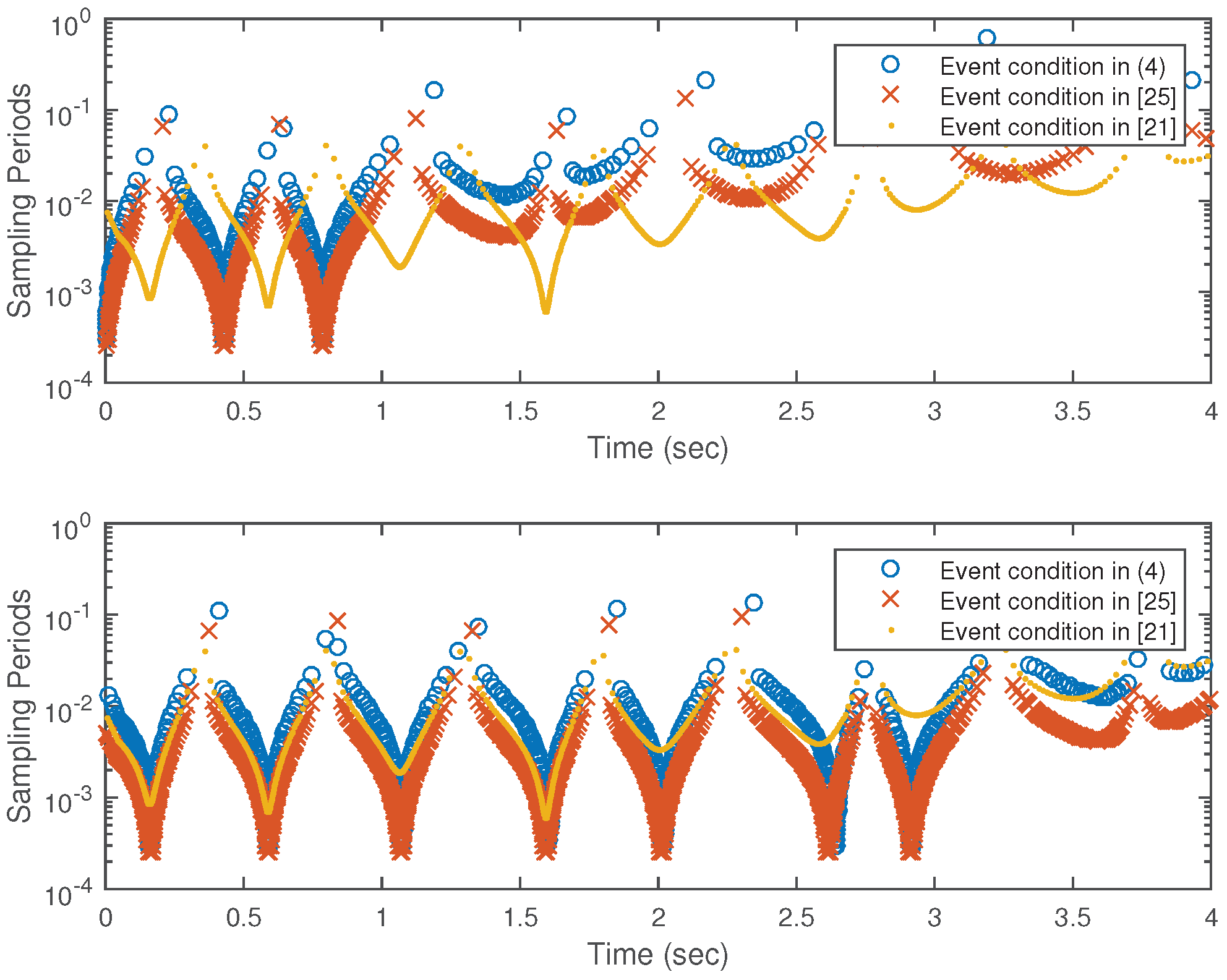
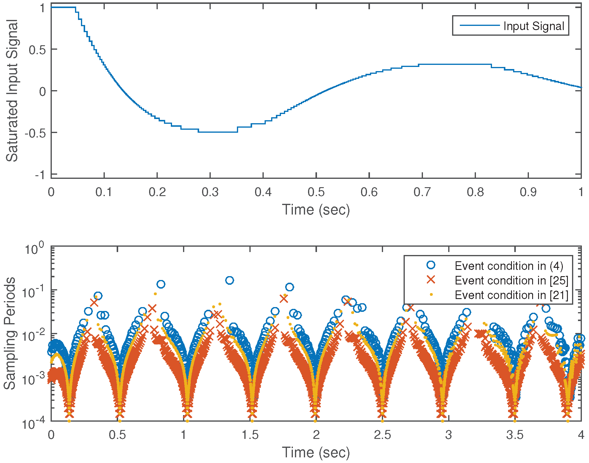
Remark 2.
The proof of Theorem 1 implies that, to guarantee the stability, one can also adopt a time-triggered control where the sampling period of sensor and actuator nodes are τ u s , s = 1 , , p and τ y l , l = 1 , , r , respectively. Hence, for stability, the event conditions are not necessary. However, the time-triggered control is not preferable to save communication resources. As shown in the Simulation section, by introducing event-triggered control, quite a larger average inter-event time can be obtained.
For given K, L and ρ 0 , the ellipsoid Γ ( P 1 , P 2 ) describes the admissible region for initial states such that the closed-loop system is asymptotically stable. Thereby, one may expect to find the largest one among them. To define the “largest”, a measure that can reflect the geometrical size of Γ ( P 1 , P 2 ) is required. Generally, the measure is often considered as volume. However, Ref. [30] pointed out that the volume optimization can lead ellipsoids to be “flat” in some directions. On the contrary, the trace optimization yields the ellipsoids that tend to be homogeneous in all directions. Referring to [18,30], we consider the following optimization problem to find the largest ellipsoid for given K, L, ρ 0 and some ε 1 , ε 2 > 0 :
min t r ( P 1 1 + P 2 1 ) subject to ( 10 ) and ( 12 ) ,
where the optimization variables are { P 1 , P 2 , H 1 , H 2 } . However, the optimization problem (18) is nonlinear subject to P 1 1 and P 2 2 . Hence, to transfer the above problem into a linear form, we propose the following theorem, where the LMI optimization problem can be solved by the standard LMI toolbox in MATLAB (8.4.0.150421, The MathWorks, Natick, Massachusetts, United States, 2014).
Theorem 2.
The solutions to Label (18) can be obtained from the following LMI optimization problem:
min t r ( Q 1 + Q 2 ) subject to φ ¯ 11 B D j H ¯ 2 B D j + 0 B D j + K ε 2 ρ 0 Q 1 0 0 φ ¯ 22 0 L 0 0 ε 2 ρ 0 Q 2 ε 1 Q 2 ε 2 I 0 0 0 0 0 ε 2 I 0 0 0 0 ε 1 I 0 0 0 ε 2 I 0 0 ε 2 I 0 ε 1 I < 0 , j M ,
1 h ¯ l + h ¯ l Q 1 0 Q 2 0 , l = 1 , , m ,
where φ ¯ 11 = A Q 1 + B D j + K Q 1 + B D j H ¯ 1 + ( A Q 1 + B D j + K Q 1 + B D j H ¯ 1 ) T , and φ ¯ 22 = ( A L C ) Q 2 + Q 2 ( A L C ) T . The LMI variables are positive definite matrices Q 1 , Q 2 , and matrices H ¯ 1 , H 2 ¯ . h ¯ l + and h ¯ l are the l th row of H ¯ 1 and H ¯ 2 , respectively. Moreover, the solutions to Label (18) are { Q 1 1 , Q 2 1 , H ¯ 1 Q 1 1 , H ¯ 2 Q 2 1 } .
Proof of Theorem 2.
Using the Schur complement, Label (20) is equivalent to
φ ¯ 11 + ε 2 ρ 0 2 Q 1 2 B D j H ¯ 2 B D j + 0 B D j + K φ ¯ 22 + ( ε 2 ρ 0 2 + ε 1 ) Q 2 2 0 L 0 ε 2 I 0 0 ε 2 I 0 I < 0 .
Pre- and post-multiplying both sides of the above inequality by d i a g { Q 1 1 , Q 2 1 , I , I , I } , it is transformed to
Q 1 1 φ ¯ 11 Q 1 1 + ρ 0 2 I Q 1 1 B D j H ¯ 2 Q 2 1 Q 1 1 B D j + 0 Q 1 1 B D j + K Q 2 1 φ ¯ 22 Q 2 1 + ( ε 2 ρ 0 2 + ε 1 ) I 0 Q 2 1 L 0 I 0 0 I 0 ε 1 I < 0 .
By denoting P 1 = Q 1 1 , P 2 = Q 2 1 , H 1 = H ¯ 1 Q 1 1 and H 2 = H ¯ 2 Q 2 1 , Label (21) is the same as Label (10) obviously. By a similar process, it is proved that Label (20) is equivalent to Label (12) with h l + = h ¯ l + Q 1 1 and h l = h ¯ l Q 2 1 . Therefore, the proof is completed. ☐
For given gain matrices K and L, if the LMIs (10) and (12) are feasible, one can design the parameters in event condition (4) according to Theorem 1 and give the largest ellipsoid by solving the LMI optimization problem in Theorem 2. Hence, in the following, we focus attention on how to find such gain matrices, i.e., a controller synthesis jointly with the parameters in the event condition.
Theorem 3.
For the closed-loop system (5), if there exist positive definite matrices Q 1 , P 2 , matrices Y k Y L , h ¯ l + , and h l , l = 1 , , m , and a positive scalar ρ 1 such that the following LMIs hold for some ε 1 , ε 2 > 0 :
Λ 11 B D j H 2 B D j + 0 B D j + Y K ε 2 Q 1 0 Λ 22 0 Y L 0 0 ε 2 I ε 2 I 0 0 0 0 ε 2 I 0 0 0 2 ε 1 Q 1 + ε 1 I 0 0 ρ 1 I 0 ρ 1 I < 0 , j M ,
1 h ¯ l + h l Q 1 0 P 2 0 , l = 1 , , m ,
where Λ 11 = A Q 1 + B D j + Y K + B D j H ¯ 1 + ( A Q 1 + B D j + Y K + B D j H ¯ 1 ) T and Λ 22 = P 2 A Y L C + ( P 2 A Y L C ) T + ε 1 I . h ¯ l + and h l are, respectively, the l th row of H ¯ 1 and H 2 . Then, { Q 1 1 , P 2 , ρ 1 1 , h ¯ l + Q 1 1 , h l } are the solutions to the LMIs (10) and (12) with K = Y K Q 1 1 and L = P 2 1 Y L .
Proof of Theorem 3.
Due to the Schur complement and the fact that Q 1 2 2 Q 1 + I , Label (22) yields
Λ 11 + ε 2 ρ 1 1 Q 1 2 B D j H 2 B D j + 0 B D j + Y k Λ 22 + ε 2 ρ 1 1 I 0 Y L 0 ε 2 I 0 0 ε 2 I 0 ε 1 Q 1 2 < 0 .
Pre- and post-multiplying both sides of Label (24) by d i a g { Q 1 1 , I , I , I , Q 1 1 } and substituting Y K Q 1 1 = K and Y L = P 2 L into Label (24), one has that Label (24) is equivalent to
Λ ¯ 11 Q 1 1 B D j H 2 Q 1 1 B D j + 0 Q 1 1 B D j + K Λ ¯ 22 0 P 2 L 0 ε 2 I 0 0 ε 2 I 0 ε 1 I < 0 ,
where Λ ¯ 11 = Q 1 1 A + Q 1 1 B D l + K + Q 1 1 B D l H ¯ 1 Q 1 1 + ( Q 1 1 A + Q 1 1 B D l + K + Q 1 1 B D l H ¯ 1 Q 1 1 ) T + ε 2 ρ 1 1 I , and Λ ¯ 22 = P 2 ( A L C ) + ( A L C ) T P 2 + ( ε 1 + ε 2 ρ 1 1 ) I . By denoting P 1 = Q 1 1 , H 1 = H ¯ 1 Q 1 1 and ρ 0 2 = ρ 1 1 , Label (25) is the same as Label (10). This shows that Label (22) is a sufficient condition for Label (10). Similarly, by pre- and post-multiplying both sides of Label (23) by d i a g { 1 , Q 1 1 , I } , Label (23) is equivalent to Label (12). Therefore, the proof is completed. ☐
Remark 3.
In Label (10), scalars ε 1 , ε 2 > 0 are two free parameters for improving the feasibility of the LMI. To make the LMI feasible, properly large ε 1 and ε 2 are expected. On the one hand, ε 1 has a counter effect on the feasibility. In fact, as shown in the last column, for a fixed P 1 , ε 1 is expected to be large enough, which, however, may yield a large P 2 . On the other hand, for a large P 2 , as shown in the forth column, a large ε 2 is expected as well. To eliminate the effect of large ε 2 , as shown in ψ 11 , ρ 0 is required to be small enough, which can always be satisfied. Therefore, to make Label (10) feasible, large ε 1 and ε 2 are expected, although too large ε 1 and ε 2 lead ρ 0 to be very small. Since a small ρ 0 would make the event condition more easy to be triggered, small ε 1 , ε 2 are expected to improve the sampling performance. To balance the feasibility of LMIs and the sampling performance, one may follow a two-step procedure for choosing the proper free parameters. First, one should select large enough ε 1 , ε 2 such that the LMIs are feasible. Second, to obtain a large ρ 0 , one should gradually decrease the values of the free parameters until the obtained ρ 0 is satisfactory or the LMIs are not feasible. The above analysis is also applicable to the LMIs in Theorems 2 and 3.
Remark 4.
In Ref. [25], the decentralised relative event condition is employed, i.e.,
t j s + 1 s = inf t { t t j s s + τ u s | e u s > σ u s u s } , s = 1 , , p ,
t k l + 1 l = inf t { t t k l l + τ y l | e y l > σ y l y l } , l = 1 , , r .
Similar to the analysis in [15] (Theorem 2), the integral-based event condition (4) is better than the relative one to some degree.
For example, we consider the node u 1 . For the same triggering input u 1 ( t k 1 1 ) , the next triggering instant t k 1 + 1 1 decided by the relative event condition cannot be larger than that decided by Label (4). In fact, when t k 1 + 1 1 determined by the relative event condition is τ u 1 , the statement is obvious. In addition, when t k 1 + 1 1 > τ u 1 , from the relative event condition, one has that e u 1 σ u 1 u 1 for all t [ t k 1 1 , t k 1 + 1 1 ) . Clearly, the inequality also holds if one integrates on both sides. Thus, the input signal at t k 1 + 1 1 that is decided by the relative event condition would not satisfy the integral-based event condition (4), and the statement is valid.

5. Simulation

5.1. Design of Event Conditions and Controllers

In this subsection, we provide numerical simulations to illustrate the feasibility of Theorems 1 and 3. Consider the following plant borrowed from [25] with
A = 0 1 0 0 48.6 1.25 48.6 0 0 0 0 1 19.5 0 19.5 0 , B = 0 21.6 0 0 , C = 1 0 0 0 0 1 0 0 .
Hence, we suppose that there are two sensor nodes, y 1 and y 2 , and one actuator node, u 1 , in the plant. The initial states of the plant and the observer are, respectively, selected as
x T ( 0 ) = 0 4.5 0.05 1.5 ; x ^ T ( 0 ) = 0.05 5.4 0.25 1.8 .
Then, by solving the LMIs in Theorem 3 with ε 1 = 8 and ε 2 = 17 , a group of feasible solutions are ρ 0 = 0.08 , the gain matrices
K = 0.0962 0.3757 0.3768 0.2257 , L T = 8.5835 3.9595 9.1535 1.1554 1.9763 45.9760 8.6555 14.5631 ,
and the ellipsoid Γ ( P 1 , P 2 ) with
P 1 = 1.1606 0.0813 0.8561 0.1488 0.0813 0.0406 0.0401 0.0325 0.8561 0.0401 0.9802 0.0607 0.1488 0.0325 0.0607 0.1063 ,
P 2 = 9.4717 3.1637 8.4906 6.2623 3.1637 2.2400 3.3975 4.6866 8.4906 3.3975 9.4641 6.3464 6.2623 4.6866 6.3464 11.9925 .
By simple calculation, the initial states belong to the above ellipsoid. According to Theorem 1 with θ = 0.9375 , the decentralized integral-based event conditions of the sensor and actuator nodes are designed as
t j 1 + 1 1 = inf t { t t j 1 1 + 3.5000 × 10 4 | t j 1 1 t e u 1 2 d ω > 0.0025 t j 1 1 t u 1 2 d ω } ,
t k 1 + 1 1 = inf t { t t k 1 1 + 3.0000 × 10 4 | t k 1 1 t e y 1 2 d ω > 0.0020 t k 1 1 t y 1 2 d ω } ,
t k 2 + 1 2 = inf t { t t k 2 2 + 3.0000 × 10 4 | t k 2 2 t e y 2 2 d ω > 0.0020 t k 2 2 t y 2 2 d ω } .
Figure 2 shows the convergence of the plant state and the observer error at the origin. The top row of Figure 3 provides the input signal trajectory, which is saturated at the initial stage of the control process. The bottom row of Figure 3 and Figure 4 show the evolutions of the inter-event times of the actuator and sensor nodes. Table 1 provides the sampling numbers of the nodes u 1 , y 1 and y 2 of the proposed scheme. By simple calculations, the average inter-event times are 0.0044 s, 0.0119 s and 0.0048 s for, respectively, u 1 , y 1 and y 2 . All of them are quite larger than τ u 1 , τ y 1 and τ y 2 . Hence, compared to the time-triggered manner, event-triggered control can save more communication resources without loss of stability. Meanwhile, we also make a comparison among the proposed integral-based event-triggered control scheme and some existing ones, i.e., the centralized relative event-triggered control in [21] and the decentralized one in [25]. The evolutions of the inter-event times are also depicted in Figure 3 and Figure 4. Obviously, almost all of the inter-event times decided by (4) are larger than those by the decentralized relative event condition, like the analysis in Remark 4. The sampling numbers for the two schemes are given in Table 1. Although the centralized event-triggered control scheme contradicts the decentralized configuration in Figure 1, comparing it with our scheme still contributes to illustrating the advantages of integral-based event condition. As shown in Table 1, on the one hand, the sampling numbers for centralized event-triggered control in [21] are less than those for the decentralized relative event condition in [25]. This accords with the analysis in [24], that is, the decentralization would weaken the sampling performance. On the other hand, for each channel, the total samplings numbers for the proposed scheme (i.e., 900 samplings for the controller-to-actuator channel and 1162 samplings for the sensor-to-controller channel) are less than those for the scheme in [21] (i.e., 1654 samplings for the controller-to-actuator channel and 1392 samplings for the sensor-to-controller channel). This illustrates that, in this simulation, the integral-based event condition can save more communication resources than the relative event condition even though the latter operates in a centralized way. Additionally, for the proposed scheme, the sampling performance of y 1 is better than that of u 1 and y 2 . To balance the sampling performance of these nodes, one can properly decrease σ y 1 and increase σ u 1 , σ y 2 within the range decided by Theorem 1.

5.2. Optimization of the Ellipsoid for Initial States

In this subsection, we provide the simulation results about the ellipsoid Γ ( P 1 , P 2 ) . For ease of presentation, we consider the following two-dimensional plant borrowed from [21] with
A = 1.7741 0.4815 7.68374 2.0741 , B = 8 8 , C = 6 9 .
Then, according to Theorem 3, one can obtain the parameter ρ 0 and the gain matrices K , L . With ε 1 = 30 , ε 2 = 17 , a group of solutions to the LMIs in Theorem 3 are ρ 0 = 0.2 , K = ( 2.5738 , 1.2988 ) ,
L = 0.6418 2.8786 , P 1 = Q 1 1 = 1.2450 0.7870 0.7870 0.5891 , and P 2 = 73.2137 19.5689 19.5689 18.3229 .
For convenience of plotting the ellipsoid, we consider the case that the initial state of the observer in Label (2) is x ^ ( 0 ) = 0 , and correspondingly z ( 0 ) = x ( 0 ) . In this situation, the set Γ ( P 1 , P 2 ) can reduce to Γ 0 ( P 1 + P 2 ) × { ( 0 , 0 ) T } with Γ 0 ( P 1 + P 2 ) = { x T R n | x T ( P 1 + P 2 ) x 1 } . Hence, one can evaluate the size of Γ ( P 1 , P 2 ) by Γ 0 ( P 1 + P 2 ) to some degree.
More importantly, Γ 0 ( P 1 + P 2 ) is a two-dimensional ellipsoid and can be plotted in the plane.
Figure 5 shows the boundary of the ellipsoid Γ 0 ( P 1 + P 2 ) with different ρ 0 , P 1 , and P 2 . First, we plot the ellipsoid with ρ 0 = 0.2 and the original P 1 and P 2 obtained from Theorem 3. Then, according to Theorem 2, one can obtain the optimized version for ρ 0 = 0.2 , and it is plotted by the solid curve. Obviously, Theorem 2 can enlarge the ellipsoid for fixed gain matrices K and L. Moreover, Figure 5 provides the curves with the parameters obtained from Theorem 2 for different ρ 0 . The results show that the size of the ellipsoid increases by decreasing ρ 0 , which indicates that there is a trade-off between the sampling performance and the admissible region for initial states such that the closed-loop system is asymptotically stable.

6. Conclusions

This paper has focused on the decentralized integral-based event-triggered asymptotic stabilization for a continuous-time linear plant with actuator saturation and output feedback. The communications between the sensor-controller channel and those between the controller–actuator channel were both considered. The sensors and actuators are implemented in a decentralized manner and the event-triggered control is executed in a decentralized manner. For given controller gain matrices, a type of Zeno-free decentralized event condition was designed to obtain the asymptotic stability of the closed-loop systems. The positive lower bound of inter-event times was guaranteed by enforcing the event conditions not to be triggered until some fixed intervals. Then, beyond these intervals, the integral-based event conditions were employed to further improve the sampling performance. A linear optimization problem was introduced to find the largest region for initial states such that the closed-loop system is asymptotically stable. Moreover, the co-design of the parameters in event conditions and the controller gain matrices was solved by means of LMI. Finally, two numerical examples were given to illustrate the efficiency and the feasibility of the proposed results. Some extensions of this paper include applying the integral-based event-triggered control to the distributed networked control [10] or multi-agent systems [31] with actuator saturations.

Acknowledgments

This work was supported by the National Nature Science Foundation of China under Grants 61573036 and 61174057, and the Beijing Natural Science Foundation under Grant 4112034.

Author Contributions

All authors discussed the related problems and did the research. Hongguang Zhang derived the theoretical results and Hao Yu performed numerical simulations. Furthermore, Hongguang Zhang and Hao Yu prepared the manuscript. Fei Hao revised the manuscript. In all other aspects, the authors contributed equally to the manuscript.

Conflicts of Interest

The authors declare no conflict of interest.

References

  1. Laila, D.S.; Nešić, D.; Astolfi, A. Sampled-data control of nonlinear systems. In Advanced Topics in Control Systems Theory; Springer: London, UK, 2006. [Google Scholar]
  2. Heemels, W.; Sandee, J.H.; Van Den Bosch, P.P.J. Analysis of event-driven controllers for linear systems. Int. J. Control 2008, 81, 571–590. [Google Scholar] [CrossRef]
  3. Tabuada, P. Event-triggered real-time scheduling of stabilizing control tasks. IEEE Trans. Autom. Control 2007, 52, 1680–1685. [Google Scholar] [CrossRef]
  4. Wang, X.; Lemmon, M. On event design in event-triggered feedback systems. Automatica 2011, 47, 2319–2322. [Google Scholar] [CrossRef]
  5. Liu, T.; Jiang, Z. A small-gain approach to robust event-triggered control of nonlinear systems. IEEE Trans. Autom. Control 2015, 60, 2072–2085. [Google Scholar] [CrossRef]
  6. Tallapragada, P.; Chopra, N. Event-triggered dynamic outputfeedback control for LTI systems. In Proceedings of the IEEE Conference on Decision and Control (CDC), Maui, HI, USA, 10–13 December 2012; pp. 6597–6602.
  7. Chen, X.; Hao, F. Observer-based event-triggered control for certain and uncertain linear systems. IMA J. Math. Control Inf. 2013, 30, 527–542. [Google Scholar] [CrossRef]
  8. Liu, C.; Hao, F. Dynamic output-feedback control for linear systems by using event-triggered quantisation. IET Control Theory Appl. 2015, 9, 1254–1263. [Google Scholar] [CrossRef]
  9. Liu, T.; Jiang, Z. Event-based control of nonlinear systems with partial state and output feedback. Automatica 2015, 53, 10–22. [Google Scholar] [CrossRef]
  10. Liu, D.; Hao, F. Decentralized event-triggered control strategy in distributed networked system with delays. Int. J. Control Autom. Syst. 2013, 11, 33–40. [Google Scholar] [CrossRef]
  11. Zhang, X.M.; Han, Q.L. Event-triggered H control for a class of nonlinear networked control systems using novel integral inequalities. Int. J. Robust Nonlinear Control 2016. [Google Scholar] [CrossRef]
  12. Ge, X.; Han, Q.L.; Yang, F. Event-based set-membership leader-following consensus of networked multi-agent systems subject to limited communication resources and unknown-but-bounded noise. IEEE Trans. Ind. Electron. 2016. [Google Scholar] [CrossRef]
  13. Zhang, X.M.; Han, Q.L.; Yu, X. Survey on recent advances in networked control systems. IEEE Trans. Ind. Inform. 2016, 12, 1740–1752. [Google Scholar] [CrossRef]
  14. Ge, X.; Yang, F.; Han, Q.L. Distributed networked control systems: A brief overview. Inf. Sci. 2017, 380, 117–131. [Google Scholar] [CrossRef]
  15. Mousavi, S.H.; Ghodrat, M.; Marquez, H.J. Integral-based event-triggered control scheme for a general class of non-linear systems. IET Control Theory Appl. 2015, 9, 1982–1988. [Google Scholar] [CrossRef]
  16. Mousavi, S.H.; Marquez, H.J. An integral based event triggered control scheme of distributed network systems. In Proceedings of the European Control Conference (ECC), Linz, Austria, 15–17 July 2015; pp. 1724–1729.
  17. Tarbouriech, S.; Garcia, G.; Gomes da Silva, J.M., Jr.; Queinnec, I. Stability and Stabilization of Linear Systems with Saturating Actuators; Springer: Berlin, Germany, 2011. [Google Scholar]
  18. Lehmann, D.; Kiener, G.A.; Johansson, K.H. Event-triggered PI control: Saturating actuators and anti-windup compensation. In Proceedings of the IEEE 51st Annual Conference on Decision and Control (CDC), Maui, HI, USA, 10–13 December 2012; pp. 6566–6571.
  19. Kiener, G.A.; Lehmann, D.; Johansson, K.H. Actuator saturation and anti-windup compensation in event-triggered control. Discret. Event Dyn. Syst. 2014, 24, 173–197. [Google Scholar] [CrossRef]
  20. Wu, W.; Reimann, S.; Liu, S. Event-triggered control for linear systems subject to actuator saturation. In Proceedings of the IFAC World Congress, Cape Town, South Africa, 24–29 August 2014; pp. 9492–9497.
  21. Ni, W.; Zhao, P.; Wang, X.; Wang, J. Event-triggered control of linear systems with saturated inputs. Asia J. Control 2015, 17, 1–13. [Google Scholar] [CrossRef]
  22. Borgers, D.P.; Heemels, W. Event-separation properties of event-triggered control systems. IEEE Trans. Autom. Control 2014, 59, 2644–2656. [Google Scholar] [CrossRef]
  23. Mazo, M., Jr.; Tabuada, P. Decentralized event-triggered control over wireless sensor/actuator networks. IEEE Trans. Autom. Control 2011, 56, 2456–2461. [Google Scholar] [CrossRef]
  24. Donkers, M.C.F.; Heemels, W. Output-based event-triggered control with guaranteed L-gain and improved and decentralized event-triggering. IEEE Trans. Autom. Control 2012, 57, 1362–1376. [Google Scholar] [CrossRef]
  25. Etienne, L.; Gennaro, S.D.; Barbot, J.P. Event-triggered observers and observer-based controllers for a class of nonlinear systems. In Proceedings of the IEEE American Control Conference, Chicago, IL, USA, 1–3 July 2015; pp. 4717–4722.
  26. Mousavi, S.H.; Marquez, H.J. Integral-based event triggering controller design for stochastic LTI systems via convex optimization. Int. J. Control 2016, 89, 1416–1427. [Google Scholar] [CrossRef]
  27. Hu, T.; Lin, Z. Control Systems with Actuator Saturation: Analysis and Design; Springer Science & Business Media: Berlin, Germany, 2001. [Google Scholar]
  28. Boyd, S.; Vandenberghe, L. Convex Optimization; Cambridge University Press: Cambridge, UK, 2004. [Google Scholar]
  29. Khalil, H. Nonlinear Systems; Prentice Hall: Upper Saddle River, NJ, USA, 2002. [Google Scholar]
  30. Wu, W.; Sven, R.; Daniel, G.; Liu, S. Event-triggered control for discrete-time linear systems subject to bounded disturbance. Int. J. Robust Nonlinear Control 2016, 26, 1902–1918. [Google Scholar] [CrossRef]
  31. Zhang, Z.; Zhang, L.; Hao, F.; Wang, L. Distributed event-triggered consensus for multi-agent systems with quantisation. Int. J. Control 2015, 88, 1112–1122. [Google Scholar] [CrossRef]
Figure 1. Decentralized event-triggered output feedback control system with saturated inputs.
Applsci 07 00011 g001
Figure 2. Trajectories of the plant state and the observer error. (a) state trajectories; (b) observer error trajectories.
Applsci 07 00011 g002
Figure 3. (top row): input signal; (bottom row): evolutions of inter-event times in node u 1 .
Applsci 07 00011 g003
Figure 4. (top row): evolutions of inter-event times in nodes y 1 ; (bottom row): evolutions of inter-event times in nodes y 2 .
Applsci 07 00011 g004
Figure 5. The ellipsoids for the initial state.
Applsci 07 00011 g005
Table 1. Sampling numbers for different event-triggered control schemes.
NodeThe Proposed SchemeThe Scheme in [21]The Scheme in [25]
u 1 90016543180
y 1 331696748
y 2 8316961803

