Abstract
We discuss the renormalization of the polarizability of a nanoparticle in the presence of either: (1) a continuous graphene sheet; or (2) a plasmonic graphene grating, taking into account retardation effects. Our analysis demonstrates that the excitation of surface plasmon polaritons in graphene produces a large enhancement of the real and imaginary parts of the renormalized polarizability. We show that the imaginary part can be changed by a factor of up to 100 relative to its value in the absence of graphene. We also show that the resonance in the case of the grating is narrower than in the continuous sheet. In the case of the grating it is shown that the resonance can be tuned by changing the grating geometric parameters.
1. Introduction
The polarizability of a nanoparticle is a response function which relates the electric dipole moment produced in it to an externally applied electric field. The polarizability is not an intrinsic property of the nanoparticle, but actually depends on the environment which it is embedded in [1,2,3]. As such, a nanoparticle’s polarizability will be modified by the presence of an underlying substrate. The study of this problem is of significant interest, since in most experimental setups the nanoparticle (NP) is placed directly onto a dielectric substrate or at a given distance from it. In previous studies in which the radiation scattered by a dielectric NP was measured using dark-field microscopy, it was shown that the presence of the substrate leads to a redshift of the NP’s resonance with respect to the situation where the NP is in vacuum [4,5,6].
The polarizability of a nanoparticle at a given frequency is a complex quantity, with its real and imaginary parts describing, respectively, the reactive and dissipative responses of a nanoparticle subjected to an electromagnetic field. Therefore, the imaginary part of the polarizability controls the extinction and absorption cross-sections of a nanoparticle subjected to an impinging electromagnetic field [7,8]. These quantities are essential for the understanding of scattering experiments of electromagnetic radiation involving nanoparticles, either isolated or forming clusters. In particular, the former case has been a topic of much interest in the context of single-molecule or single-particle spectroscopies [9,10]. The knowledge of the imaginary part of the polarizability is also essential in order to understand the phenomena of blackbody and thermal friction experienced by a neutral nanoparticle in close proximity to an interface between two media [11]. It is therefore of major importance to understand how the imaginary part of the polarizability is renormalized relative to its value in a vacuum when it is near an interface, the most common setup in experiments.
It would be of particular relevance (from the device engineering viewpoint), if the dielectric properties of the interface, near which the nanoparticle is located, could be tuned. This would provide a route for controlling the value of the nanoparticle polarizability in real time. Such an approach is not viable when we consider the interface between two conventional dielectrics or between a metal and a dielectric, since the interface has fixed properties by construction. Fortunately, there is a possible and technologically feasible route to overcome this limitation. Adding a graphene sheet between an interface involving two different dielectrics provides an additional degree of freedom to the problem. Indeed, the Fermi energy of a graphene sheet can be controlled in real time using a gate. Tuning the Fermi energy of graphene changes the local dielectric environment around the nanoparticle and therefore the value of the imaginary part of the nanoparticle polarizability. This is the opportunity we will explore in this paper.
Incidentally, the problem of nanoparticle polarizability renormalization in the presence of a substrate is also relevant for the characterization of the dielectric properties of a scanning near-field optical microscope (SNOM). Scanning near-field optical microscopy is a technique frequently used to image and characterize surface polaritons in graphene [12] and other two-dimensional materials, such as boron nitride [13]. More recently, exciton-polaritons have also been studied in layered transition metal dichalcogenides using the same method [14]. Indeed, the SNOM tip is frequently modeled as a dipole, as is the nanoparticle [15]. Therefore, understanding how a nanoparticle changes its dielectric properties under illumination allows us to also understand the problem of a SNOM tip illuminated with THz radiation during the excitation of surface polaritons in graphene and other two-dimensional materials.
In this work, we study the renormalization of a nanoparticle polarizability located near the interface between two dielectrics interspaced with a doped graphene sheet, or with an array of graphene ribbons (see Figure 1). One of the dielectrics is the vacuum and the other acts as substrate for the support of the graphene sheet. In order to keep the analysis simple we shall restrict ourselves to the case of a non-dispersive and non-dissipative substrate, characterized by a frequency-independent and real dielectric constant. We explore the imaginary part of the polarizability in the THz range of the electromagnetic spectrum, a spectral region where graphene supports surface plasmon polaritons [16,17,18]. As we will see, the excitation of these polaritons leads to a significant change of the polarizability of both metallic and semiconductor nanoparticles. Indeed, the bare polarizability of a metallic nanoparticle in vacuum is essentially constant in the THz, with a very small imaginary part. However, when located near a graphene sheet, the polarizability undergoes strong renormalization, especially with respect to its imaginary part.
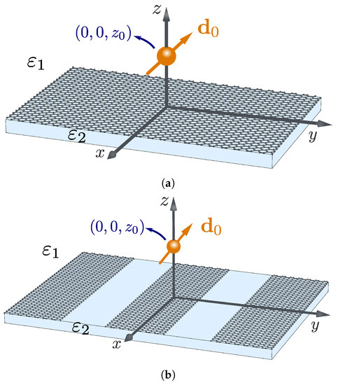
Figure 1.
The two systems considered in this paper: a graphene sheet (a) and a graphene grid of ribbons (b) located in between two dielectrics. A nanoparticle is located at position and is characterized by a polarizability tensor in vacuum. In addition, a plane wave impinges on the nanoparticle and on graphene coming from .
Although the problem of modeling the polarizability of a nanoparticle close to a graphene sheet has been considered before by some of the authors of the present paper [19], that work relied on a electrostatic approximation. The present work goes beyond that, taking into account retardation effects, allowing us to correctly describe the imaginary part of the polarizability. It should be noted that the problem of determining the nanoparticle’s polarizability in the presence of a homogeneous flat dielectric substrate has also been considered previously both in the electrostatic approximation [20] and in the full electrodynamic approach [6,21,22].
The goals of this work are as follows: (1) to extend the study of [19] including retardation effects, thus using a more general formalism; (2) to bring together in a single paper a formalism that is scattered in the literature using many different notations; (3) to introduce a rigorous formulation of the dyadic Green’s function formalism that is absent in many papers; and (4) to extend this approach to the case where a nanoparticle has both dipolar electric and dipolar magnetic moments.
This paper is organized as follows: in Section 2 we introduce the concept of dyadic Green’s function for the electric field as a tool to obtain the electric field in the presence of source currents. In Section 2.1 we study in detail the electric field dyadic Green’s function in free-space (or in a homogeneous medium). The Weyl’s, or angular spectrum, representation of the dyadic Green’s function is introduced in Section 2.2. This representation is well-suited to deal with the problem of radiation scattering at planar interfaces. It is also shown that the dyadic Green’s functions can be expressed in terms of the tensor product of the electric field s- and p-polarization vectors. In Section 2.3, we focus on the problem of scattering at a planar interface and define the reflected and transmitted Green’s functions. In Section 3 we deduce the polarizability of a nanoparticle close to an interface covered by graphene. We start defining and studying the polarizability of a nanoparticle embedded in a vacuum, in Section 3.1. The approach is generalized in Section 3.2 to the case of a nanoparticle close to a planar interface. This general description is then used to describe the renormalization of a nanoparticle’s polarizability close to a continuous graphene sheet and to a graphene grating in Section 3.3 and Section 3.4. In Section 4 we present a generalization of the formalism to the case where the nanoparticle has both electric and magnetic dipole moments. Such a magnetic moment can be generated, even for nanoparticles formed by a non-magnetic material, due to induced currents inside the nanoparticle [23], and can actually be the main contribution for the polarizability in the case of dielectric NPs [4,5,6]. Finally, a set of appendices provides some auxiliary results.
2. Dyadic Green’s Function for the Electric Field
2.1. Free-Space Dyadic Green’s Function
The goal of this section is to introduce the necessary tools to study the polarizability of a nanoparticle in the presence of substrate. In particular, we will introduce the electric field dyadic Green’s function, which allows us to solve the wave equation for the electric field in the presence of source currents. Although the material in this section is relatively well-known, we present it here in some detail both for the sake of completeness and to fix notations used throughout the paper.
In frequency space, the dyadic Green’s function, , allows us to express the total electric field, , in the presence of a source current, , as
where is the electric field in the absence of the source current, is vacuum’s permeability, and is the relative permeability of the medium where the source current is embedded in. If the source current is due to a point dipole located at , we have that , where is the electric dipole moment. In this case, Equation (1) reduces to (for )
In order to determine the dyadic Green’s function we will follow a method originally described in [24]. The first step to determining in this approach is noticing that in the presence of a source current, the wave equation for the electric field can be written as an inhomogeneous Helmholtz equation (see Appendix A for a derivation) as follows:
where we have introduce the quantity , where is the speed of light in the medium, is the vacuum’s permittivity, and is the medium relative dielectric constant. The general solution of the Helmholtz equation can be written as (see Appendix B)
where
is the Green’s function for the scalar Helmholtz equation [1,24,25] and represents integration in the principal value sense, where an infinitesimal volume, , enclosing the point is excluded. We have written with ⊗ denoting the tensor product and the prime indicates that the derivative acts on variables. The Helmholtz Green’s function is the solution of
in a way that is clarified in Appendix B. Notice that is integrable, and therefore, the exclusion of the volume is not usually emphasized. However, it will be important when determining the behaviour of when . Although Equation (4) already allows us to compute the electric field as a function of the current, it is useful to obtain an alternative expression which does not involve derivatives of the current. Such an expression can be obtained by carefully performing integration by parts. It must the noticed that due to the excluded volume surrounding , boundary terms are generated when doing this. In particular we have that
where is a outward-pointing unit vector, normal to the surface of the enclosing volume . In the limit of infinitesimal excluded volume, the first term of the above equation vanishes, since the element of area scales as , while . For the second term, we perform integration by parts once again. For clarity we explicitly write the tensorial components in a Cartesian basis, with repeated induces being summed over, and obtain
Now the boundary term is finite. In the limit of an infinitesimal volume, we take , such that and use the limit of Equation (A26). This allows us to write
where the dyadic is defined as [24]
which can be interpreted as a depolarization term. Therefore, Equation (4) can be written in the form of Equation (1) with the dyadic Green’s function, , given by
where indicates that the small volume centered at is to be excluded. Notice that depends on the shape of the chosen excluded volume [24]. For a sphere, it is straightforward to show that . In this case, the free-space dyadic Green’s function in real space can be written as the sum of four terms [26,27]:
respectively, the far-, intermediate-, near- and self-field terms, which are written as
where the terms , and are to be understood in the principal value sense, and we have introduced the definitions and .
We point out that in more standard derivations of the dyadic Green’s function it is easy to miss the depolarization term Equation (9) [1,28], or fail to recognize its dependence on the shape of the excluded volume [29,30]. It will be shown in Section 3 that this term is crucial to correctly capture self-field contributions to a particle polarizability. The dependence of depolarization term on the shape of the volume is also important when dealing with non-spherical particles. An alternative derivation of the depolarization term Equation (9) based on the vector potential can be found in [31].
2.2. Weyl’s or Angular Spectrum Representation of the Dyadic Green’s Function: A Useful Formulation for Interfaces
Although Equation (10) can be used directly to evaluate , for many applications such formulation might not be the most useful. In the the case of scattering by planar interfaces it is useful to make a (two-dimensional) Fourier transform of the fields in the coordinates parallel to the interface. This representation of the fields and of the Green’s function is generally referred to as Weyl’s or angular spectrum representation. In this representation, the electric field is written as
where is the in-plane wave-vector and are in-plane coordinates. In this representation Equation (4) becomes
where is the Weyl representation of the current density, defined in analogous way to Equation (16), , , ⨏ represents the principal value integral in one dimension, excluding the point , and is the Helmholtz Green’s function in the Weyl representation, defined such that
The function can be easily obtained from the components of the three-dimensional Fourier transform of the Helmholtz Green’s function, , as
This integral can be easily performed by contour integration yielding
where is defined as
Clearly, Equation (20) is written is terms of both propagating and evanescent waves [32]. Similarly to what we have done in the previous section, we can rewrite Equation (17) by moving the derivatives from to . Doing this yields
with being the dyadic Green’s function in Weyl’s representation
where we have introduced , with the ± sign applying for . The last term in the above equation is the depolarization term, that arises from the boundary contributions when performing integration by parts, due to the exclusion of an infinitesimal line element around in ⨏. The principal value in the first term indicates that a small region around is to be excluded. We also notice that this depolarization term could also have been obtained from the general depolarization dyadic in real space, Equation (9), if we choose as excluded volume an infinite slab located at (with ). For this excluded volume, we would obtain .
It is possible to write Equation (23) in a more meaningful way by introducing the s- and p-polarization vectors. The s-polarization vector lies in the plane and is therefore written as [33]
On the other hand, the p-polarization vector is orthogonal to and , and therefore we write it as [33]
where is the p-polarization vector for a field propagating in the positive/negative direction. With these definitions we have that and, therefore, we can write Equation (23) as [34,35]
with the first and the second terms corresponding to the s- and p-polarization components of the free-space dyadic Green’s function, respectively. A different derivation of previous two equations has been given in the literature previously [36,37,38]. The same decomposition has been used in the study of an emitter’s life-time near a graphene sheet [39,40] and in the context of the calculation of the electric field of a dipole near graphene [41].
2.3. Source and Scattered Green’s Functions: Scattering at a Planar Interface
We now want to address the problem of determining the Green’s function in a system with a planar interface between media 1 and 2. To that end, we shall evaluate the electric field generated by a point dipole, characterized by an electric dipole moment , located at a distance from the interface. We assume that medium 1 is located in the half-space , whereas medium 2 is located in the complementary space, as represented in Figure 1. Note that in general due to the different values of the speed of light in the media. Assuming that , the primary field emitted by the oscillating dipole in the half-space reads
We have two different values for the field, depending on whether . Recalling Equation (26) we obtain
with s- and p-polarization amplitudes being given by
This field corresponds to waves impinging on the interface at , being partially reflected and partially transmitted as depicted in Figure 2. The reflected and transmitted fields can be expressed in terms of the amplitudes of the incident field at and of the reflection, and , and transmission, and , coefficients at the interface for the s- and p-polarizations as [33,35]

Figure 2.
Representation of the primary field (), emitted by a point dipole (represented by the golden ball with an arrow), and the reflected () and the transmitted () field due to the presence of the interface at . The ± sign in indicates whether the field is emitted along the positive/negative z direction.
The factor is acquired by the field while propagating along the positive (negative) z direction in medium 1 (2). The p-polarization vector for the reflected field is since it propagates along the positive z direction. Conversely, we have for the transmitted field, since it propagates along the negative z direction.
Therefore, the total field for can be written as
where we have introduced the reflected Green’s function
Similarly, the transmitted field for can be written as
with the transmitted Green’s function being written as
At this point, we have now in our possession all the relevant tools to study the renormalization of the polarizability of a nanoparticle in the vicinity of a planar interface.
3. Renormalization of the Polarizability of a Quantum Emitter Near a Graphene Sheet and a Graphene-Based Grating
The dyadic Green’s function method is a powerful tool for describing the modification of the properties of a quantum emitter near interfaces, as it takes into account the change in the density of electromagnetic modes induced by the presence of the interface. Problems such as the calculation of the Purcell factor and Förster energy transfer are two examples [42,43] well-suited for the Green’s function approach. Here we consider another problem that also depends on the density of electromagnetic modes, the calculation of the effective polarizability of a quantum emitter.
3.1. Polarizability of a Quantum Emitter in a Homogeneous Medium
The polarizability of a nanoparticle, , treated as a point object, relates the electric dipole moment, , that is induced in the nanoparticle to the value of the externally applied electric field, , at the nanoparticle’s position, , via
Note that does not include self-field effects, that is, the electric field generated by the nanoparticle itself when subjected to . Let us consider a homogeneous medium characterized by and , in which a nanoparticle with dielectric function lives. Then, the electric field obeys Equation (1) with the free current due to the nanoparticle polarization (excluding the current due to the polarization density of the homogeneous medium) being written as
where we have used the usual linear constitutive relation . is the polarization density due to the nanoparticle, is the polarization density due to the homogeneous medium, and is the total electric field in the nanoparticle. Therefore, from Equation (1), the electric field obeys a Lippmann–Schwinger equation [44]
where is a solution of the wave equation in the homogeneous medium, and V is the volume of the nanoparticle. We want to solve for the electric field inside the nanoparticle. We will follow the approximate approach of [22]. We shall assume a spherical nanoparticle, with radius R, and assume that . This allows us to approximate as being constant inside the nanoparticle and to take the limit for . Taking into account Equations (12)–(14), in the limit we can write the regular part (excluding the Dirac -function term) of the free-space dyadic Green’s function as
where . We neglect the real part of when compared to , thereby approximating
Using the above approximation in Equation (39) and assuming that the electric field within the nanoparticle varies slowly, that is, throughout V, we can solve the obtained algebraic equation for the total field as a function of the external field , obtaining
Therefore, the electric dipole moment follows from
where we have introduced the Clausius–Mossotti polarizability [45]
The polarizability of a nanoparticle embedded in a homogeneous medium with relative permittivity can be read from Equation (43)
It must be pointed out that the above equation is only approximate. As a matter of fact it is easy to see that if we had kept the term in we would have generated a real term, , in the denominator of Equation (45), which can be interpreted as a dynamic depolarization effect [46]. The obtained term would still be incorrect, as additional terms of the same order in would appear from taking into account that the electric field inside the nanoparticle is not constant. An exact treatment using Mie’s scattering theory for a spherical particle would lead to [45,47]
There is indeed a term of order , but the term of order is unchanged. The imaginary term of order is usually denoted by radiation damping correction [1,48] and is essentially to enforce the optical theorem for electromagnetic scattering in the lowest order [1,49,50,51]. We note in passing that the radiation damping correction is also responsible for the decay rate of the dipole [1]. In the next sections, we will ignore the term of order as it plays no significant role. However, it will become clear that it is essential to keep the radiation damping correction.
3.2. Polarizability of a Quantum Emitter in Proximity to a Planar Interface
If the nanoparticle is situated in the vicinity of an interface, it is also possible to write an equation of the Lippmann–Schwinger type for the electric field similar to Equation (39). The only difference is that in order to take into account the interface, the free-space dyadic Green’s function must be replaced by the one which incorporates the reflection from the substrate, . Likewise, the external field must be replaced by a solution of the electric field wave equation in the presence of the substrate, , where is the incident field and is the reflected field. Therefore, the Lippmann–Schwinger equation for the electric field taking into account the substrate is given by
We now proceed in the same fashion as before, assuming , approximating as constant inside the nanoparticle, and keeping only the dominant contributions from in the limit . Therefore, we write [22]
where we have used the fact that is regular. Introducing Equation (48) into Equation (47), and approximating , we can solve for as a function of , obtaining
The electric dipole moment is thus given by
with the effective polarizability defined as
This equation can be expressed in terms of the free-space polarizability Equation (45) as
Equation (51) has been derived in the literature before, following a similar argumentation [6,21,22].
The importance of keeping the free-space radiation damping correction, , will now become clear. According to Poynting’s theorem, the power dissipated by the nanoparticle is given by
This implies that the imaginary part of the diagonal components of must be positive, since the dissipated power must be positive. It is easily checked that if a and g are complex quantities then If , but a is otherwise arbitrary, the requirement that implies that . Translating this into the problem of the polarizability, since we have that in general , the requirement that demands that . This is true only for the complete Green’s function, following from the general properties of Green’s functions, and can be understood either classically as the fact that gives the total power emitted by a point dipole, or quantum mechanically, since the diagonal elements or correspond to a spectral function (a density of electromagnetic states), that is always positive. However, it will not be true in general that is positive. As a matter of fact, it becomes negative in situations where subradiance of a quantum emitter occurs. Therefore, the requirement that , forces us to keep the free-space radiation damping correction.
3.3. Renormalized Polarizability of an Isotropic Quantum Emitter Near a Continuous Graphene Sheet
In what follows we shall consider the case of an isotropic quantum emitter in close proximity to a graphene sheet. In the previous sections, we have seen how the effective polarizability of a nanoparticle depends on the reflected Green’s function, , which can be reconstructed from its angular spectrum representation as
As shown in Section 2.3, the reflected Green’s function in the angular spectrum representation can be written in terms of the Fresnel reflection coefficients. For a planar interface covered by graphene, the reflection coefficients are given by [18,52]
where and are the transverse and longitudinal optical conductivities of graphene and given by Equation (21). Neglecting nonlocal effects in the conductivities we have , which we will model with a Drude-like term [18,53,54]
where is graphene’s Fermi energy and is the broadening factor. The transmission coefficients and are related to the reflection coefficients via [18]
After performing the integration over the angular variable in Equation (54), we find that is diagonal. Rotational invariance along the z direction imposes that , which will differ from . The same will be true for the polarizability of the nanoparticle, which, using Equation (51), we can write as
where we have defined the dimensionless quantities with the diagonal element of the nanoparticle polarizability from Equation (45). and .
More explicitly, these quantities can be evaluated from
where .
Some insight on the previous expressions can be obtained by estimating them in the electrostatic limit, valid for . In this limit, the main contribution is due to the reflection coefficient. Approximating we obtain
with the reflection coefficient being approximated by
where we have approximated and have introduced the graphene’s surface plasmon polariton complex wavenumber
and is the fine structure constant. From these results we can already estimate when the effect of the graphene substrate on the NP polarizability will be more significant. From Equation (65), is peaked at , while the term in the integrand of Equation (64) has a maximum at . Therefore, will have a maximum when these two peaks coincide, [43] which occurs for . In the electrostatic limit, Equation (64) can be written in terms of known functions as
where the function is given by
with the exponential integral function, which for a real positive argument is written as However, we point out that Equation (67) is valid even in the presence of finite broadening in graphene.
We shall consider both metallic and polar semiconductor nanoparticles, with the relative dielectric function described, respectively, by the Drude and Lorentz models. The Drude model for the dielectric function reads
where is the metal’s plasma frequency and is the relaxation rate, while the Lorentz model for the dielectric function of a polar material is given by
where and are the frequencies of the transverse and longitudinal optical phonons, is a phonon decay rate, and is the high frequency limit of the dielectric function. As examples of commonly used materials for the production of nanoparticles, we consider gold (metallic) and CdSe (polar semiconducing) nanoparticles. Typical values of the polarizability for different substances are given in [55]. The used values for the Lorentz model of CdSe are taken from [56].
In Figure 3 we depict the real and imaginary parts of the polarizability of a gold nanoparticle near a doped graphene sheet on a substrate with . The figure clearly shows the strong renormalization of the polarizability of the nanoparticle relative to its value in the presence of the interface without graphene (blue dashed line). This is due to the close proximity of the nanoparticle to the graphene sheet, nm (compared to the typical free-space wavelengths in the THz range). Nowadays, with the ubiquitous use of hexagonal boron nitride (h-BN) for encapsulating graphene, together with the possibility of controlling the number of layers of h-BN, it poses no difficulty to routinely produce structures where nanoparticles are positioned very close to the graphene sheet, that is, at distances much smaller than their radius. Also, the -component of the polarizability tensor (black dotted line) is renormalized differently from the -component (red solid line). This is a consequence of breaking the translation symmetry along the z–direction introduced by the graphene sheet and the dielectric change as we cross the plane. We have verified that the broadband resonance seen in the imaginary part of the polarizability tensor is due to the excitation of surface plasmon polaritons in graphene. This was assessed studying the dispersion of the resonance as a function of the Fermi energy (more on this below).
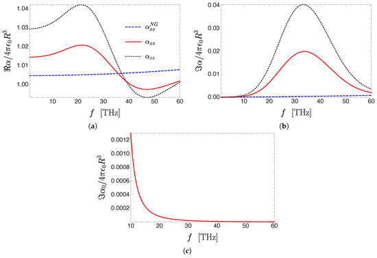
Figure 3.
Top panels: Real (a) and imaginary (b) parts of the renormalized polarizability of a gold nanoparticle with radius nm located at a distance of nm from a graphene sheet with a Fermi energy of 1 eV and damping parameter of meV supported by a dielectric of permittivity . The solid red line represents the component, and the black dotted line represents the component of the polarizability in the presence of graphene. For comparison, the component of the polarizability of the nanoparticle is also represented in the absence of graphene (but in the presence of the dielectric interface), as . One can appreciate the increase in the imaginary part of the polarizability by about two orders of magnitude when the particle is near doped graphene. (c) The imaginary part of the nanoparticle polarizability in a vacuum. In all the panels, the parameters used in the Drude model for dielectric function of gold are: eV and eV.
Given the close proximity of the nanoparticle to the graphene sheet, the question of the necessity of a nonlocal description of the graphene conductivity arises. In order to check the correctness of our local description, we have performed simulations (results not shown) using the nonlocal Drude-like conductivity [18] of graphene. We have found that nonlocal effects in the graphene conductivity (its dependence on the wavevector) play no visible role in the position or the intensity of the resonance in the effective polarizability of the nanoparticle (when nm). We also expect nonlocal effects akin to the nanoparticle to be negligible provided that nm, below which nonlocal contributions in metallic nanoparticles usually arise [57,58] (the situation is different for semiconductor nanoparticles [58]).
In Figure 4 we present the spectrum of the polarizability of a CdSe nanoparticle in the presence of graphene on a substrate. As in Figure 3, the observed broad band resonance in the imaginary part of the polarizability tensor components is due to the excitation of surface plasmons in graphene. As discussed previously, the order of magnitude of the plasmonic resonance frequency can be estimated from the relation , which is independent of the nanoparticle’s material. Indeed, we observe the resonance here approximately at the same frequency as for the metallic nanoparticle (see Figure 3). In order to further access the plasmonic nature of the broad band resonance, we have studied its position as a function of the Fermi energy and found a complete agreement with the above relation, that is, in the peak of the resonance scales with the Fermi energy . Interestingly, the intensity of the resonance in Figure 4 is smaller by a factor of 2.5 when compared to the case of the metallic nanoparticle. This can be understood from the following simple consideration. We notice that in the imaginary part of the bare polarizability, is negligible for both metallic and CdSe nanoparticles in the considered frequency range. Therefore, we can write for the imaginary part of the renormalized polarizability (e.g., the component):

Figure 4.
Real (a) and imaginary (b) parts of the renormalized polarizability of a CdSe nanoparticle with nm located at a distance of nm from a graphene sheet with a Fermi energy of 1 eV and damping parameter of meV, supported by a dielectric of permittivity . The solid red line represents the component of the polarizability, and the black dotted line represents the component. The dashed blue line is the component of the polarizability in the absence of graphene. The parameters used in both panels for the Lorentz model for the dielectric function of CdSe are: , cm, cm and cm.
Since for 15 THz, we have for CdSe, while for the metal particles , because the metal permittivity is negative and large in modulus in the far-infrared region. The denominator is close to unity in both cases, so in the case of a metal nanoparticle, we have a stronger renormalization of the polarizability (by a factor of ≈2.5) in the presence of a graphene sheet. This is the maximum renormalization that one can obtain if the bare polarizability is dispersionless. In contrast to metals, a nanoparticle made of CdSe has a dipolar mode due to optical phonons, which occurs at the so-called Fröhlich frequency (unless the particle’s size is so small that it gives rise to quantum confinement effects, of the order of few nanometers) [59], , which is equal to ≈6 THz in this case. When the plasmonic resonance overlaps with , the phonon resonance in the nanoparticle is greatly enhanced because at . In this case, a non-trivial dependence on the Fermi energy takes place [19]. Note that none of these effects would take place in the presence of a metallic substrate for the same studied spectral range, as plasmons in metals at these frequencies are essentially free radiation.
3.4. Renormalized Polarizability of an Isotropic Quantum Emitter Near a Plasmonic Graphene Grating
In this section we revisit the problem of the renormalization of the polarizability of a quantum emitter now considering it near a plasmonic graphene grating. The used procedure is only approximate, relying on a semi-analytic approach. However, the analysis performed is sufficient to capture the effect of plasmonic resonances of the graphene grating in the nanoparticle polarizability.
3.4.1. Optical Properties of a Plasmonic Graphene Grating
For a metamaterial such as the graphene-based grating depicted in Figure 1b, the description of the interaction of the material with a quantum emitter can be quite complex. One possible method for overcoming such a difficulty is by computing the effective conductivity of the metamaterial, in this case the plasmonic graphene grating. The general method for accomplishing this was given in [60] and was later applied to the problem of tuning total absorption in graphene [61], but no details of its calculation were given. Instrumental to the calculation of the effective conductivity is the knowledge of the reflection and transmission Fresnel coefficients. These coefficients were computed in approximated analytical form in [62] and we give here only the final results:
where and are the reflection and transmission coefficients, respectively, of the zero diffraction-order of the grating (the only propagating order for a sub-wavelength grating), w is the width of the graphene ribbons in the grating, L is the period of the grating, and the function reads
which encodes the information about the plasmonic resonance in the grating. With given by
where and , with , is the Bessel function of order 1. Here, the summation in is delicate due to the oscillatory nature of the Bessel function (see [62]). For simplicity of the calculation, we approximate by . In addition to and there is an infinite number of other coefficients associated with higher diffraction order, but they are all evanescent in nature for the parameters chosen in the figures. Therefore, we approximate the optical properties of the grating considering only and , and and (we have checked that introducing more evanescent terms does not change the results). This gives us an analytical description of its optical properties. As noted above, from the knowledge of and , and and we can derive an effective conductivity for the graphene grating along the direction perpendicular to the axis of the graphene ribbon. This effective conductivity shows a maximum in its real part associated with the excitation of surface plasmon polaritons. The same information is encoded in the function , as can be seen in Figure 5 and, in fact, for our analysis this latter function is all we need for including plasmonic effects into the calculation.
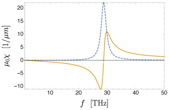
Figure 5.
Real (blue dashed line) and imaginary (orange line) of the function . The parameters of the grating are m and . The Fermi energy of graphene is eV. The real part has a pronounced resonance due to the excitation of a surface plasmon polariton of that frequency (∼87 THz).
Notice that the conductivity of the system is no longer isotropic. Therefore, we will introduce this anisotropy in an effective way, choosing different Fermi energies for the and reflection coefficients. Also, while the coefficients are given by Equation (72), the coefficient is given by Equation (55). This procedure renders our results qualitative and no quantitative agreement is expected with an exact calculation. The exact solution would require us to extend the formalism to the case on a non-isotropic system in the plane. Note that this system has broken rotational symmetry around the axis. Therefore, we expected that the equality seen in the case of continuous graphene sheet should not hold in the case of grating. Our qualitative results show that this is indeed the case.
3.4.2. Renormalization of the Polarizability of a Quantum Emitter
In this section we study the renormalization of the polarizability of a quantum emitter near a plasmonic graphene-based grating. As explained above, we use the reflection coefficients and in the reflected p–Green’s function and an effective Fermi energy, given by in the coefficient in Equation (55), and use this in the reflected s-Green’s function. We consider only the case of a metallic nanoparticle, as the results are qualitatively the same for a semiconductor one. In Figure 6 we depict the real and imaginary parts of the renormalized polarizability of a gold nanoparticle in the proximity of a graphene-based grating. A strong renormalization of the real part of the polarizability can be seen at the same frequency where the grating supports the excitation of surface plasmon polaritons (see Figure 5). The same happens in the imaginary part. However, the relative change of the imaginary part is much larger than for the real part. The results for the imaginary part of the polarizability in the case of grating should be compared to those given in Figure 3 for the same quantity. For the continuous sheet the enhancement of the imaginary part of is about that found in the present case. This is attributed to the approximate description of the reflection coefficients of the grating. Indeed, we would expect the renormalization to be larger in the case of the grating as the latter supports excitation of plasmons by far-field radiation, whereas in the case of the continuous graphene sheet the excitation of plasmons is due to near-field excitation only. We also note that the resonance peak in the imaginary part of the polarizability is not of broad band when compared to the same quantity in the continuous case.
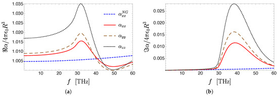
Figure 6.
Real (a) and imaginary (b) renormalized polarizability of a gold nanoparticle in close proximity to a plasmonic graphene-based grating. The solid red line represents the component of the polarizability in the presence of graphene, the dashed brown line represents the component, and the black dotted line represents the component. The dashed blue line is the component of the polarizability in the absence of graphene. Note that , due to lack of rotational symmetry in the plane introduced by the ribbon structure. The parameters of the grating are m and . The parameters for the graphene conductivity and for the Drude dielectric function of gold are the same as in Figure 3.
On other hand, the frequency where the maximum of the resonance is located is larger in the present case. This happens since we can tune the position of the resonance in the grating by varying both the Fermi energy and the geometric parameters of the grating. Therefore, the grating system has a versatility that cannot be found in the continuous sheet case. Indeed, using gratings with smaller periods, the resonance can be tuned across the electromagnetic spectrum, from the THz spectra to the infrared. We also note that the renormalization of component (black dotted line) is substantially larger than the component (red solid line) and the one (brown dashed line). This happens because the component of the Green’s function is about twice as large compared to the component.
As noted above, tuning the grating parameters allows for an additional degree of freedom to control the impact of graphene on the polarizability of a nanoparticle. The tuning can be twofold: (1) changing the period of the grating and keeping the aspect ratio to 1/2 (constant filling factor); and (2) changing the aspect ratio, keeping the period fixed. In the first case, the procedure allows for large changes in the spectral position of the resonance; this is because the momentum of the SPP is essentially . Since the SPP dispersion is proportional to , L fixes the position of the resonance. In the second case, a fine tuning of the position of the resonance is achieved. However, the effect of the renormalization of the polarizability is greater for the half-filled case. This is because in this regime the plasmonic resonance has the maximum intensity [16,62]
Finally, we have verified that when , we recover the results of a continuous graphene sheet.
4. Extension of the Formalism When the Quantum Emitter Has Both an Electric and a Magnetic Dipole
A current density of a particle can be described in terms of its moments in a multipole expansion [63]. A small particle, however, can often be described using only the multipole moments of the lowest orders. In the case of a metallic nanoparticle, its response is dominated by the electric dipole moment. Nevertheless, it is known that in some cases it is necessary to go beyond the electric dipole approximation and consider higher-order moments [6]. In particular, it has been shown that silicon nanoparticles with size between the tens and hundreds of nanometers can have strong responses in the infrared and visible spectra due to higher order moments [4,5,6,23,64], with the magnetic dipole moment contributing the most, even though the particles are not magnetic by themselves. This motivates us to generalize the formalism of the previous sections to the case of a point-like nanoparticle (or quantum emitter) with both electric and magnetic dipole moments. Although the Green’s functions technique has been used before in this problem [6,15,38], some details regarding the behavior of the Green’s functions at coincidence, that is, when , have been overlooked. Therefore, we carefully present the full formalism, that is, accounting for both electric and magnetic dipole contributions, below.
4.1. Free-Space Electric, Magnetic and Mixed Green’s Functions
Our starting points are the inhomogeneous Helmholtz equations for the electric and the magnetic fields (in fact the magnetic field induction ) in the presence of a source current density (see Appendix A for the derivation):
As before, we can write the solution for the inhomogeneous Helmholtz equations as
In the same spirit of Equation (38), we write the current in terms of polarization, , and magnetization, , densities as
Inserting the latter result into Equations (78) and (79) we obtain
where we have used the fact that and . We now proceed as in Section 2.1, using integration by parts, while taking into account the boundary terms due to the excluded volume enclosing the point , in the same form that we have already dealt with for the electric field Green’s function. The crossed terms relating the magnetization to the electric field and the polarization to the magnetic field only involve one derivative of the Helmholtz Green’s function and therefore the generated boundary term vanishes in the limit of infinitesimal excluded volume. Therefore, we may simply write
where we have used the fact that in a translation-invariant system . Finally, the term that relates the magnetization to the magnetic field (magnetic field induction) can be treated in a similar way as the one for the electric field Green’s function. The only difference is that we also have to use integration by parts for the Laplacian term. The steps to treat this term are exactly the same as the ones to treat the term in Section 2.1 and we obtain
where is given by Equation (9) and , (see Equation (A28)). This quantity is just the solid angle of excluded volume centered at divided by , which equals 1 for any surface (see Appendix B). We also point out that for we have . These results allow us to write
where we have the electric field and magnetic field Green’s functions
and we have the mixed Green’s functions defined as
These describe magnetoelectric effects, which can be important when the nanoparticle sits on a substrate [6]. The dyadic in Equation (88) can be interpreted as a demagnetization term. For the case for a spherically-symmetric excluded volume, we have . The factor of is well-known as being the demagnetization factor of a spherical particle [63], however, to the best of our knowledge, this term has not been discussed in the literature before in the context of the application of Green’s functions to electromagnetic problems. Correctly taking this term into account is essentially to describe self-field effects in the magnetization of a particle (analogous to the self-field effects in the polarization in the (electric-only) case considered before).
For the case of nanoparticle characterized by a permittivity and permeability , the free polarization and magnetization densities inside the nanoparticle volume read
where and are the polarization densities of the nanoparticle and host medium, and and are their densities, respectively. We used the linear constitutive relations and . The previous relation between the magnetic field induction and the magnetization follows from the equations and , where is the magnetic susceptibility, then . The same reasoning provides the relation between the polarization and the electric field. Inserting the two previous equations in Equations (85) and (86), we obtain
4.2. Weyl’s or Angular Spectrum Representation of Magnetic and Mixed Green’s Functions
Now we will see what is the Weyl’s (or angular spectrum) representation of the magnetic and mixed Green’s functions. The magnetic Green’s function is almost the same as the electric Green’s function, the only difference being the different additional self-field term, which is isotropic and independent of the chosen excluded volume. Therefore, we can write
We point out that the demagnetization term was previously obtained in [38]. As for the mixed Green’s function, their Weyl’s representation can be obtained by making the replacements: , and for . Therefore, we obtain
where for . As for the electric and the magnetic Green’s functions, the mixed Green’s functions in the Weyl representation can also be written in terms of the s- and p-polarization vectors. It is straightforward to verify that
which allows us to write
This representation is useful, as it allows for a simple interpretation of the emitted fields generated by the electric and magnetic dipoles in terms of s- and p–polarized electromagnetic waves.
If we are interested in the problem of scattering at a planar interface between two dielectric media with for , and for , we can construct reflected and transmitted Green’s functions expressed in terms of reflection and transmission coefficients, as done previously for . However, some care must be taken in what the polarization vectors mean in the Green’s function, considering that the polarization of an electromagnetic field is usually defined by the polarization of the field. The quantity gives us the electric field generated by a point magnetic dipole located at . Therefore, the reflected and transmitted Green’s functions are constructed in the same way as for , and for we obtain
For the magnetic Green’s functions, and , we must take into account that these describe a field generated by, respectively, a point magnetic and electric dipole. For electric and magnetic dipoles, and , located at , the primary magnetic field emitted for is given by
with
The corresponding electric field can be obtained from Maxwell’s equations as . More explicitly (for ) we have for the primary field
This primary electric field is scattered by the interface at , giving origin to a reflected field for , which reads
and to a transmitted field for
The corresponding magnetic fields can be obtaining using Faraday’s law applied to Equations (104) and (105). For example: if then , where and is the amplitude of the s-component of the field. The obtained magnetic fields are given by
From the above Equations (106) and (107), we can, after replacing Equations (101) and (102) in Equations (106) and (107), obtain the reflected and transmitted magnetic Green’s functions, which are given by
Notice that the Fresnel reflection and transmission coefficients are defined for the electric field. With the last four equations we conclude the development of the formalism for the calculation of the renormalized polarizability [6] of a nanoparticle possessing both electric and magnetic dipoles.
5. Conclusions
In this paper we have studied the influence of two plasmonic structures on the effective polarizability of a nanoparticle made of either a metal (with a nearly dispersionless bare polarizability) or a polar dielectric or semiconductor (with a resonant polarizability due to polar optical phonons). The two studied structures are a continuous graphene sheet and a plasmonic graphene-based grating. In both cases a significant enhancement of the imaginary part of the polarizability has been observed. The two media possess plasmonic resonances which, however, occur at different frequencies. In the particular case of the grating, the resonance is tunable in two different ways: by adjusting the gate voltage and by changing the geometric parameters of the grating. In this case, it is possible to scan the resonance from the THz to the mid-IR range, whereas for the continuous graphene sheet the resonance is always in the THz range for the currently achieved values of electronic doping using a gate. The approach pursued here was to model the nanoparticle by a point-like dipole. The main motivation for this approach lies in its ability to make analytic progress. However, in real systems, one has a finite-size particle which can be modeled as an assembly of many point-like dipoles. These are determined by the coupled dipole equations [49]. In this case, the particle, even a spherical one, has other multipole resonances that can couple to the incoming radiation and contribute to the extinction cross-section. The two lowest multipoles, besides the electric dipole, are the magnetic dipole and the electric quadrupole. It can be shown numerically that for semiconductor nanoparticles such as spheres, cubes, pyramids, disks, and cylinders, the extinction cross-section has a strong magnetic-dipole resonance [4,5,6,23]. We note, however, that for semiconductor nanoparticles, if we consider interband transitions, that is, exciton resonances that are characteristic of semiconductors, the relevance of higher multipole resonances depends much more on the underlying band structure than on the shape. The formalism used in this paper to describe the renormalization of the electric dipole resonances can be extended to include the problem of magnetic dipole resonance [6], as we have seen in the previous section. The contribution to the extinction cross section of the magnetic dipole is given by , where is the power per unit area of the incoming radiation and , with being the effective magnetic polarizability of the particle and the incoming magnetic field. The effective magnetic polarizability can be derived as done before for the electric dipole case. To that end, we will need the dyadic magnetic Green’s function which can be obtained by writing the wave equation for the magnetic field using the procedure outlined in Section 4. This study will be pursued in a forthcoming paper.
Acknowledgments
B.A. received funding from the European Union’s Horizon 2020 research and innovation programme under grant agreement No 706538. N.M.R.P. and M.I.V. acknowledge useful discussions with Jaime Santos and support from the European Commission through the project “Graphene-Driven Revolutions in ICT and Beyond” (Ref. No. 696656) and the Portuguese Foundation for Science and Technology (FCT) in the framework of the Strategic Financing UID/FIS/04650/2013. P.A.D.G. acknowledges fruitful discussions with N. Asger Mortensen. The Center for Nanostructured Graphene is funded by the Danish National Research Foundation (project DNRF103).
Author Contributions
B.A. and N.M.R.P. did the calculations, and drafted the first version of the manuscript. P.A.D.G. performed calculations without the self-field, and contributed to the analysis and discussion of all results. M.I.V. contributed in the discussion and critical analysis of the results. All authors contributed equally to the discussion of the results and writing of the final version of the paper.
Conflicts of Interest
The authors declare no conflict of interest
Abbreviations
The following abbreviations are used in this manuscript:
| SNOM | Scanning near-fieldoptical microscope |
| RHS | Right-hand-side |
| NP | Nanoparticle |
| THz | Terahertz |
Appendix A. Derivation of the Wave Equation
Let us start revising the basics of electromagnetic theory writing Maxwell’s equations for a homogeneous medium of relative dielectric permittivity and relative permeability :
The free current density (current per unit volume) and the free charge density (charge per unit volume) are linked via the continuity equation:
By free, we mean those currents that are not already taken into account by the polarization an magnetization densities included in electric displacement, , and in the magnetic strength field, . The connection between the displacement and electric fields, and between the magnetic induction and magnetic strength fields is given by (for linear media)
where and are the medium relative permittivity and permeability, respectively. Taking the curl of Equation (A1) and using Equation (A2) we obtain the wave equation for the electric field
where is the speed of light in the medium. Let us now consider harmonic fields with a time dependence . In this case, the wave equation reads
Taking the curl of Equation (A2) we find a wave equation for the magnetic induction
Considering a harmonic time dependence of the fields and of the current it follows that
It is possible to rewrite Equations (A9) and (A11) as inhomogeneous Helmholtz equations. In order to do so, we make use of the identity and write Equations (A9) and (A11) as
Next, we use Equation (A4) to write , and Equations (A2) and (A6) to write . Using the continuity Equation (A5), the free charge density can be written in terms of the free current density, as . Therefore, we have that the electric and magnetic fields obey the inhomogeneous Helmholtz equations
The solution to these equations can be expressed in terms of the Green’s function for the Helmholtz equation.
Appendix B. Green’s Function for the Helmholtz Equation
The inhomogeneous scalar Helmholtz equation for a field and non-homogeneous source term is given by
The solution for this equation can be expressed in terms of the Helmholtz Green’s function as
where is a particular solution of the Helmholtz equation, , is the retarded Helmholtz Green’s function, which is given by Equation (5) (we have dropped the frequency argument), and excludes an infinitesimal volume enclosing the point . The goal of this appendix is to prove that Equation (A17) with given by Equation (5) is indeed a solution of the inhomogeneous Helmholtz equation. In order to do that we will first solve Equation (A16) by decomposing it in terms of Fourier components, allowing a simple derivation of . However, that derivation does not clarify how the integration in Equation (A17) should be performed. Therefore, we will also prove that Equation (A17) solves the inhomogeneous Helmholtz equation by direct substitution.
Writing all the fields in Fourier components
and similarly for , Equation (A16) becomes an algebraic equation with solution given by , where
is the Helmholtz Green’s function in Fourier space. Inverting the Fourier transform, we can write
with [25,65]
In order to evaluate this integral we make the replacement in order to obtain a retarded response function. The angular integration is easily performed and yields
The remaining integration over p can be performed using contour integration techniques, by closing the contour on the upper complex half-plane and collecting the residue at and obtain Equation (5). Notice that in order to close the integral into the upper half-plane we must assume that . Next, we will prove by direct substitution that Equation (A17) with the Green’s function given by the above equation solves the inhomogeneous Helmholtz equation (Equation (A16)). By doing so, we will check that the integration in Equation (A17) actually excludes the point .
The crucial point in proving that Equation (A17) actually solves the inhomogeneous Helmholtz equation is to notice that the integration region over is actually a function of . Therefore, we can write
where is the surface of the infinitesimal volume centered at and is a outwards pointing unit vector, normal to . In the limit of an infinitesimal volume element the boundary term in the above equation vanishes: if is the characteristic linear size of , then we have while . Therefore, we can write
The boundary term now actually gives a finite contribution. To see that, first we notice that in the limit of an infinitesimal volume we have that and therefore we can replace . Next we notice that
such that we can approximate for
Therefore we can write
where
Therefore, if we act directly with on Equation (A17) we obtain
The first term in the first line is zero, since is a solution of the homogeneous Helmholtz equation, while the first term in the last line is zero, since for . Therefore, we obtain
Next we notice that the quantity is actually 1 and is independent of the shape of the excluded volume, . First we notice that is actually just the solid angle of the surface that encloses the point divided by . For a sphere, the solid angle is and therefore . For any other surface, we notice that the solid angle is just the flux of the vector field
which satisfies for . Therefore, for any volume enclosing the point , we can consider a enclosed sphere () and then write
Since in the volume (the volume excluding the enclosing sphere) the field is regular, we can use the divergence theorem and obtain that the last term of the above equation is zero.
Therefore, we have obtained not only the explicit form of the Helmholtz Green’s function but have also shown that Equation (A17) is a solution of the inhomogeneous Helmholtz equation, emphasizing the role played by the excluded volume in the integration of . In the case of a vector Helmholtz equation, we can use a Cartesian basis and then use the scalar Helmholtz equation for each of the components.
References
References
- Novotny, L.; Hecht, B. Principles of Nano-Optics, 2nd ed.; Cambridge University Press: Cambridge, UK, 2012. [Google Scholar]
- Pelton, M.; Bryant, G.W. Introduction to Metal-Nanoparticle Plasmonics; John Wiley & Sons: Hoboken, NJ, USA, 2013; Volume 5. [Google Scholar]
- Amendola, V.; Pilot, R.; Frasconi, M.; Maragò, O.M.; Iatì, M.A. Surface plasmon resonance in gold nanoparticles: A review. J. Phys. Condens. Matter 2017, 29, 203002. [Google Scholar] [CrossRef] [PubMed]
- Evlyukhin, A.B.; Novikov, S.M.; Zywietz, U.; Eriksen, R.L.; Reinhardt, C.; Bozhevolnyi, S.I.; Chichkov, B.N. Demonstration of Magnetic Dipole Resonances of Dielectric Nanospheres in the Visible Region. Nano Lett. 2012, 12, 3749–3755. [Google Scholar] [CrossRef] [PubMed]
- Kuznetsov, A.I.; Miroshnichenko, A.E.; Fu, Y.H.; Zhang, J.; Luk’yanchuk, B. Magnetic light. Sci. Rep. 2012, 2. [Google Scholar] [CrossRef] [PubMed]
- Soshnichenko, A.E.; Evlyukhin, A.B.; Kivshar, Y.S.; Chichkov, B.N. Substrate-Induced Resonant Magnetoelectric Effects for Dielectric Nanoparticles. ACS Photonics 2015, 2, 1423–1428. [Google Scholar] [CrossRef]
- Barnes, W.L. Particle plasmons: Why shape matters. Am. J. Phys. 2016, 84, 593–601. [Google Scholar] [CrossRef]
- Gonçalves, M.R. Plasmonic nanoparticles: fabrication, simulation and experiments. J. Phys. D Appl. Phys. 2014, 47, 213001. [Google Scholar] [CrossRef]
- Slaughter, L.S.; Chang, W.S.; Swanglap, P.; Tcherniak, A.; Khanal, B.P.; Zubarev, E.R.; Link, S. Single-Particle Spectroscopy of Gold Nanorods beyond the Quasi-Static Limit: Varying the Width at Constant Aspect Ratio. J. Phys. Chem. C 2010, 114, 4934–4938. [Google Scholar] [CrossRef]
- Slaughter, L.; Chang, W.S.; Link, S. Characterizing Plasmons in Nanoparticles and Their Assemblies with Single Particle Spectroscopy. J. Phys. Chem. Lett. 2011, 2, 2015–2023. [Google Scholar] [CrossRef]
- Jentschura, U.D.; Łach, G.; De Kieviet, M.; Pachucki, K. One-Loop Dominance in the Imaginary Part of the Polarizability: Application to Blackbody and Noncontact van der Waals Friction. Phys. Rev. Lett. 2015, 114, 043001. [Google Scholar] [CrossRef] [PubMed]
- Chen, J.; Badioli, M.; Alonso-Gonzalez, P.; Thongrattanasiri, S.; Huth, F.; Osmond, J.; Spasenovic, M.; Centeno, A.; Pesquera, A.; Godignon, P.; et al. Optical nano-imaging of gate-tunable graphene plasmons. Nature 2012, 478, 77–81. [Google Scholar] [CrossRef] [PubMed]
- Dai, S.; Fei, Z.; Ma, Q.; Rodin, A.S.; Wagner, M.; McLeod, A.S.; Liu, M.K.; Gannett, W.; Regan, W.; Watanabe, K.; et al. Tunable Phonon Polaritons in Atomically Thin van der Waals Crystals of Boron Nitride. Science 2014, 343, 1125–1129. [Google Scholar] [CrossRef] [PubMed]
- Hu, F.; Luan, Y.; Scott, M.; Yan, J.; Mandrus, D.; Xu, X.; Fei, Z. Imaging exciton–polariton transport in MoSe2 waveguides. Nat. Photonics 2017, 11, 356–360. [Google Scholar] [CrossRef]
- Joulain, K.; Ben-Abdallah, P.; Chapuis, P.O.; Babuty, A.; De Wilde, Y. Tip-sample electromagnetic interaction in the infrared: Effective polarizabilities, retarded image dipole model and near-field thermal radiation detection. arXiv, 2012; arXiv:physics.optics/1201.4834. [Google Scholar]
- Bludov, Y.V.; Ferreira, A.; Peres, N.M.R.; Vasilevskiy, M.I. A Primer on Surface Plasmon-Polaritons in Graphene. Int. J. Mod. Phys. B 2013, 27, 1341001. [Google Scholar] [CrossRef]
- Sorger, C.; Preu, S.; Schmidt, J.; Winnerl, S.; Bludov, Y.V.; Peres, N.M.R.; Vasilevskiy, M.I.; Weber, H.B. Terahertz response of patterned epitaxial graphene. New J. Phys. 1015, 17, 053045. [Google Scholar] [CrossRef]
- Gonçalves, P.A.D.; Peres, N.M.R. An Introduction to Graphene Plasmonics; World Scientific: Singapore, 2016. [Google Scholar]
- Santos, J.E.; Vasilevskiy, M.I.; Peres, N.M.R.; Smirnov, G.; Bludov, Y.V. Renormalization of nanoparticle polarizability in the vicinity of a graphene-covered interface. Phys. Rev. B 2014, 90, 235420. [Google Scholar] [CrossRef]
- Wind, M.; Vlieger, J.; Bedeaux, D. The polarizability of a truncated sphere on a substrate I. Phys. A Stat. Mech. Appl. 1987, 141, 33–57. [Google Scholar] [CrossRef]
- Hakkarainen, T.; Setälä, T.; Friberg, A.T. Electromagnetic near-field interactions of a dipolar emitter with metal and metamaterial nanoslabs. Phys. Rev. A 2011, 84, 033849. [Google Scholar] [CrossRef]
- Dahan, N.; Greffet, J.J. Enhanced scattering and absorption due to the presence of a particle close to an interface. Opt. Express 2012, 20, A530–A544. [Google Scholar] [CrossRef] [PubMed]
- Evlyukhin, A.B.; Reinhardt, C.; Chichkov, B.N. Multipole light scattering by nonspherical nanoparticles in the discrete dipole approximation. Phys. Rev. B 2011, 84, 235429. [Google Scholar] [CrossRef]
- Yaghjian, A.D. Electric dyadic Green’s functions in the source region. Proc. IEEE 1980, 68, 248–263. [Google Scholar] [CrossRef]
- Duffy, D.G. Green’s Functions with Applications, 2nd ed.; CRC Press: Boca Raton, FL, USA, 2015. [Google Scholar]
- Arnoldus, H.F. Transverse and longitudinal components of the optical self-, near-, middle- and far-field. J. Mod. Opt. 2003, 50, 755–770. [Google Scholar] [CrossRef]
- Frahm, C.P. Some novel delta-function identities. Am. J. Phys. 1983, 51, 826–829. [Google Scholar] [CrossRef]
- Tai, C.T. Dyadic Green Functions in Electromagnetic Theory, 2nd ed.; Institute of Electrical & Electronics Engineers (IEEE): New York, NY, USA, 1994. [Google Scholar]
- Collin, R.E. Field Theory of Guided Waves; Wiley: New York, NY, USA, 1990. [Google Scholar]
- Born, M.; Wolf, E. Principles of Optics: Electromagnetic Theory of Propagation, Interference and Diffraction of Light, 7th ed.; Cambridge University Press: Cambridge, UK, 1999. [Google Scholar]
- Rothwell, E.J.; Cloud, M.J. Electromagnetics; CRC Press: Boca Raton, FL, USA, 2001. [Google Scholar]
- Setälä, T.; Kaivola, M.; Friberg, A.T. Decomposition of the point-dipole field into homogeneous and evanescent parts. Phys. Rev. E 1999, 59, 1200–1206. [Google Scholar] [CrossRef]
- Arnoldus, H.F.; Foley, J.T. Transmission of dipole radiation through interfaces and the phenomenon of anti critical angles. J. Opt. Soc. Am. A 2004, 21, 1109–1117. [Google Scholar] [CrossRef]
- Pieplow, G.; Haakh, R.H.; Henkel, C. A Note on longitudinal fields in the Weyl expansion of the electromagnetic Green tensor. Int. J. Mod. Phys. Conf. Ser. 2012, 14, 460–466. [Google Scholar]
- Arnoldus, H.F.; Berg, M.J. Energy transport in the near field of an electric dipole near a layer of material. J. Mod. Opt. 2015, 62, 218–228. [Google Scholar] [CrossRef]
- Bedeaux, D.; Mazur, P. On the critical behaviour of the dielectric constant for a nonpolar fluid. Physica 1973, 67, 23–54. [Google Scholar] [CrossRef]
- Sipe, J. The ATR spectra of multipole surface plasmons. Surf. Sci. 1979, 84, 75–105. [Google Scholar] [CrossRef]
- Sipe, J.E. New Green-function formalism for surface optics. J. Opt. Soc. Am. B 1987, 4, 481–489. [Google Scholar] [CrossRef]
- Nikitin, A.Y.; Guinea, F.; Garcia-Vidal, F.J.; Martin-Moreno, L. Fields radiated by a nanoemitter in a graphene sheet. Phys. Rev. B 2011, 84, 195446. [Google Scholar] [CrossRef]
- Nikitin, A.Y.; Guinea, F.; Garcia-Vidal, F.J.; Martin-Moreno, L. Analytical Expressions for the Electromagnetic Dyadic Green’s Function in Graphene and Thin Layers. IEEE J. Sel. Top. Quantum Electron. 2013, 19, 4600611. [Google Scholar] [CrossRef]
- Hanson, G.W. Dyadic Green’s functions and guided surface waves for a surface conductivity model of graphene. J. Appl. Phys. 2008, 103, 064302. [Google Scholar] [CrossRef]
- Biehs, S.A.; Agarwal, G.S. Large enhancement of Förster resonance energy transfer on graphene platforms. App. Phys. Lett. 2013, 103, 243112. [Google Scholar] [CrossRef]
- Kort-Kamp, W.J.M.; Amorim, B.; Bastos, G.; Pinheiro, F.A.; Rosa, F.S.S.; Peres, N.M.R.; Farina, C. Active magneto-optical control of spontaneous emission in graphene. Phys. Rev. B 2015, 92, 205415. [Google Scholar] [CrossRef]
- Yang, T.R.; Dvoynenko, M.M.; Goncharenko, A.V.; Lozovski, V.Z. An exact solution of the Lippmann–Schwinger equation in one dimension. Am. J. Phys. 2003, 71, 64–71. [Google Scholar] [CrossRef]
- Capolino, F. Theory and Phenomena of Metamaterials; CRC Press: Boca Raton, FL, USA, 2009. [Google Scholar]
- Meier, M.; Wokaun, A. Enhanced fields on large metal particles: dynamic depolarization. Opt. Lett. 1983, 8, 581–583. [Google Scholar] [CrossRef] [PubMed]
- Ru, E.L.; Etchegoin, P. Principles of Surface Enhanced Raman Spectroscopy and Related Plasmonic Effects; Elsevier: Amsterdam, The Netherlands, 2009. [Google Scholar]
- Carminati, R.; Greffet, J.J.; Henkel, C.; Vigoureux, J. Radiative and non-radiative decay of a single molecule close to a metallic nanoparticle. Opt. Commun. 2006, 261, 368–375. [Google Scholar] [CrossRef]
- Draine, B.T.; Flatau, P.J. Discrete-Dipole Approximation For Scattering Calculations. J. Opt. Soc. Am. A 1994, 11, 1491–1499. [Google Scholar] [CrossRef]
- D’Agostino, S.; Sala, F.D.; Andreani, L. Radiative coupling of high-order plasmonic modes with far-field. Photonics Nanostruct.-Fundam. Appl. 2013, 11, 335–344. [Google Scholar] [CrossRef]
- Stauber, T.; Gómez-Santos, G.; de Abajo, F.J.G. Extraordinary Absorption of Decorated Undoped Graphene. Phys. Rev. Lett. 2014, 112, 077401. [Google Scholar] [CrossRef] [PubMed]
- Bludov, Y.V.; Peres, N.M.R.; Vasilevskiy, M.I. Unusual reflection of electromagnetic radiation from a stack of graphene layers at oblique incidence. J. Opt. 2013, 15, 114004. [Google Scholar] [CrossRef]
- Peres, N.M.R.; Lopes dos Santos, J.M.B.; Stauber, T. Phenomenological study of the electronic transport coefficients of graphene. Phys. Rev. B 2007, 76, 073412. [Google Scholar] [CrossRef]
- Stauber, T.; Peres, N.M.R.; Guinea, F. Electronic transport in graphene: A semiclassical approach including midgap states. Phys. Rev. B 2007, 76, 205423. [Google Scholar] [CrossRef]
- Haynes, W.M. Handbook of Chemistry and Physics, 93rd ed.; CRC Press: Boca Raton, FL, USA, 2012. [Google Scholar]
- Hamma, M.; Miranda, R.P.; Vasilevskiy, M.I.; Zorkani, I. Calculation of the Huang–Rhys parameter in spherical quantum dots: the optical deformation potential effect. J. Phys. Condens. Matter 2007, 19, 346215. [Google Scholar] [CrossRef]
- David, C.; de Abajo, F.J.G. Nonlocal Effects in the Optical Response of Metal Nanoparticles. AIP Conf. Proc. 2010, 1291, 43–45. [Google Scholar]
- Maack, J.R.; Mortensen, N.A.; Wubs, M. Size-dependent nonlocal effects in plasmonic semiconductor particles. EPL (Europhys. Lett.) 2017, 119, 17003. [Google Scholar] [CrossRef]
- Vasilevskiy, M.I. Dipolar vibrational modes in spherical semiconductor quantum dots. Phys. Rev. B 2002, 66, 195326. [Google Scholar] [CrossRef]
- Tassin, P.; Koschny, T.; Soukoulis, C.M. Effective material parameter retrieval for thin sheets: Theory and application to graphene, thin silver films, and single-layer metamaterials. Phys. B Condens. Matter 2012, 407, 4062–4065. [Google Scholar] [CrossRef]
- Fan, Y.; Liu, Z.; Zhang, F.; Zhao, Q.; Wei, Z.; Fu, Q.; Li, J.; Gu, C.; Li, H. Tunable mid-infrared coherent perfect absorption in a graphene meta-surface. Sci. Rep. 2015, 5, 13956. [Google Scholar] [CrossRef] [PubMed]
- Gonçalves, P.A.D.; Dias, E.J.C.; Bludov, Y.V.; Peres, N.M.R. Modeling the excitation of graphene plasmons in periodic grids of graphene ribbons: An analytical approach. Phys. Rev. B 2016, 94, 195421. [Google Scholar] [CrossRef]
- Jackson, J.D. Classical Electrodynamics, 3rd ed.; Wiley: Hoboken, NJ, USA, 1999. [Google Scholar]
- García-Etxarri, A.; Gómez-Medina, R.; Froufe-Pérez, L.S.; López, C.; Chantada, L.; Scheffold, F.; Aizpurua, J.; Nieto-Vesperinas, M.; Sáenz, J.J. Strong magnetic response of submicron Silicon particles in the infrared. Opt. Express 2011, 19, 4815–4826. [Google Scholar] [CrossRef] [PubMed]
- Desanto, J. Scalar Wave Theory: Green’s Functions and Applications; Springer: Berlin, Germany, 1992. [Google Scholar]
© 2017 by the authors. Licensee MDPI, Basel, Switzerland. This article is an open access article distributed under the terms and conditions of the Creative Commons Attribution (CC BY) license (http://creativecommons.org/licenses/by/4.0/).