Enhanced Prognostic Model for Lithium Ion Batteries Based on Particle Filter State Transition Model Modification

Abstract

This paper focuses on predicting the End of Life and End of Discharge of Lithium ion batteries using a battery capacity fade model and a battery discharge model. The proposed framework will be able to estimate the Remaining Useful Life (RUL) and the Remaining charge through capacity fade and discharge models. A particle filter is implemented that estimates the battery’s State of Charge (SOC) and State of Life (SOL) by utilizing the battery’s physical data such as voltage, temperature, and current measurements. The accuracy of the prognostic framework has been improved by enhancing the particle filter state transition model to incorporate different environmental and loading conditions without retuning the model parameters. The effect of capacity fade in the reduction of the EOD (End of Discharge) time with cycling has also been included, integrating both EOL (End of Life) and EOD prediction models in order to get more accuracy in the estimations.

1. Introduction

Lithium ion batteries are widely used in spacecraft, aircraft, and electric vehicles. Hence, an accurate prognosis for the remaining useful life (RUL) and time until end of discharge voltage (EODV) is essential for these applications [1]. Significant research has been conducted in order to get higher energy density, reduced weight and cost, longer life, or shorter recharge times [2]. New materials and technologies are continually being explored with the goals of improving the technology and satisfying consumer requirements. The ability to precisely monitor and manage battery health will increase the performance and avoid catastrophic failures, mainly in aerospace systems. The failure of a battery can lead to loss of operation, reduced competency, stoppage, and even catastrophic failure [3]. There are two main prognostic and health management approaches: physics of failure and data driven. Physics of failure prognostic methods utilize knowledge of a product’s life cycle, loading conditions, geometry, material properties, and failure mechanisms to predict its RUL [4].

Data-driven techniques extract features from performance data such as current, voltage, time, and impedance using statistical and machine learning techniques to track the product’s degradation and estimate its RUL [5]. The current state of a battery is usually indicated by two common indices, namely state-of-charge (SOC) and state of health (SOH). SOC is quantified as the percentage of charge remaining in a battery before recharging during the current cycle. SOH indicates the RUL of a battery [6].

The particle filter (PF) has been extensively used in estimating the RUL of lithium ion batteries [6,7,8,9,10,11,12]. Particle filters are sequential Monte Carlo methods that track and predict the state of the system [13]. He et al. [7] proposed a novel approach to predict the state of health (SOH) and RUL using the Dempster–Shafer theory (DST) and the Bayesian Monte Carlo (BMC) method. An empirical model based on the physical degradation behaviour of lithium ion batteries was developed. DST was used to initialize the model parameters by combining sets of training data, and BMC was used to update the model parameters and evaluate the RUL. Saha and Goebel [14] presented an empirical model to describe battery behavior during individual discharge cycles as well as over its life cycle. Consequently, the model has been used in a particle filter framework to predict the RUL for individual discharge cycles as well as for cycle life. An extension to He et al.’s [7] work was proposed by Xing et al. [6] by testing an empirical second-order polynomial model for RUL predictions and compared it with He el al.’s particle filter model. Their results showed that the particle filter predicted the RUL more accurately than the polynomial model. Dalal et al. [15] used a lumped parameter battery model to perform diagnostics on lithium ion batteries. Their work was similar to Saha and Goebel [14] in regards to the state transition model in EOD predictions. The particle filter has been widely used in prognostics of other applications. Daigle et al. [16] used a physics-based model of a centrifugal pump combined with PF in predicting the failure of a pump. This research involves the development of an improved prognostic model to determine End of Life (EOL) and End of Discharge (EOD), thus increasing the accuracy of the RUL prediction of the lithium ion batteries. Wang et al. [17] performed prognostics on lithium ion batteries based on battery performance analysis and flexible support vector regression (F-SVR). In their research, energy efficiency and working temperature were used as the input data and they discovered that the non-iterative prediction model based on F-SVR is suitable for long-term prediction, whereas an iterative multi-step prediction model based on SVR is suitable for short-term predictions. Tang et al. [18] used the Wiener process with measurement error to predict the RUL estimation of lithium ion batteries with nonlinear degradation. They also found that the relaxation effect could lead to the recovery of the battery (i.e., increases the available capacity for the next cycle). Qin et al. [19] signified the importance of state of health (SOH) prognostics for safe and reliable use of lithium ion batteries; and then proposed a rest time-based prognostic framework (RTPF) in which the beginning time interval of two adjacent cycles is adopted to reflect the rest time, in order the accurately predict the regeneration phenomena and improve long-term prediction performance of battery SOH. Huang et al. [20] performed a fractional impedance diagnosis on a commercial NCM/graphite lithium ion battery at various SOC values to investigate deformation behaviors, charge transfer functions, and SEI layer statuses. Their analytical results showed that when SOC ≤ 26.5%, both charge transfer resistance and diffusion impedance increased significantly with decreasing SOC values, thus suggesting that automotive Li-ion batteries for electric vehicles should work in DOD below 80%.

Analysis of current battery prognostic techniques proved that further work will be required to increase the accuracy of the prognostic accuracy. The basis of the present work is the prognostic model developed by Saha and Goebel [14]. However, this study enhances the particle filter state transition model during EOD prediction, making it adaptable to different environmental and loading conditions without retuning the model parameters. The effect of capacity fade in the reduction of the EOD time with cycling has also been included, integrating both EOL and EOD prediction models in order to get more accuracy in the estimations.

2. Failure Modes of Lithium Ion Batteries

This section will provide an overview of the different modes of failure of lithium ion batteries.

2.1. Battery Cell Shelf Discharge

This type of failure only occurs when the battery is stored. A battery is considered to be in storage conditions when it is not being used as well as when it is connected, but not cycled. Ambient temperature, storage time, and the battery state of charge are the main parameters that affect the shelf discharge rate [21]. The cell degradation rate may increase due to storing the battery at high temperatures and/or high SOC conditions. The battery internal impedance increases and the battery capacity is reduced due to the relationship between battery capacity and internal impedance.

2.2. Thermal Runway

This type of failure is considered to be one of the most dangerous failures that can occur in a battery and usually originates at the cell level. It involves an accelerated shelf-heating of the cell, which is initiated due to chemical reactions between the positive and negative electrodes. This usually ends with a fire or explosion of the battery [22]. Thermal runways usually occur during or shortly after charging, when the cell cannot dissipate all the excess heat created.

2.3. Cell Imbalance

Cell imbalance is a common occurrence in a battery module or system that is categorized by a different state of charge of the cells constituting the package. Multi-cell configurations involving series and parallel connections are usually utilized in meeting the application current and voltage requirements and, despite the efforts at manufacturing identical cells, they usually exhibit different behavior within the same battery module. This difference can lead to cell overcharging, over-discharging or internal currents flowing inside the battery package. Cell imbalance is usually exhibited by a variance in cell voltage, and techniques such as cell bypassing during charge/discharge have been utilized [23]. In addition, the battery management and thermal management systems that monitor and control the battery components can minimize the effects of cell imbalance.

2.4. Capacity Fade

Capacity fade can be defined as the reduction in the maximum amount of charge that can be stored or extracted from a battery [24]. The ideal failure of a battery is slow capacity fade, which is mainly caused by aging. The result of this would be the growth of internal impedance. The battery is considered to be in a failed state when the nominal capacity has been reduced by 20% from its nominal value. The main factors that contribute to capacity fading are: aging, temperature, and charging or discharging patterns [25,26]. The ability to predict battery capacity fade and evaluate the RUL could result in safer and more effective use of lithium ion batteries.

2.5. Power Fade

While capacity fade refers to the reduction of cell or battery capacity as it ages, power fade is related to the inability of the battery to supply the power required by the system or application. Both failure modes, capacity and power fade, are closely correlated because of the previously-stated relationship between capacity and impedance.

As can be deduced from Equation (1), an increase in the impedance will cause a reduction in the power that the battery can supply. Thus, cell impedance should be monitored in order to evaluate the degradation of the battery.

$$P=I·V=I^2·Z=\frac{V^2}{Z}$$

(1)

Table 1. Summary of battery failure modes.

Failure Mode	Level	Primary Causes	Symptoms	Comments	Parameter to Monitor
Shelf discharge	Cell	-High ambient temperatures both during usage and storage	-Loss of capacity -Increase in the cell internal impedance		-SOC -Temperature
Thermal runaway	Cell	-Internal or external short circuit of a cell -High temperature operation (overheating) -Overcharging	-Cell heating during charging, especially near the end of charging -High voltage drop during rest periods -Charge capacity higher than discharge capacity	-The failure originates at cell level but it can propagate to the other cells composing the system. -The rate at which heat is produced in the system exceeds the rate at which it can be dissipated.	-Temperature -Cell Voltage -SOC
Cell capacity imbalance	Module/System	-Different behaviour of cells within the same module	-Different cell voltages	-Occurs when the SOC of different cells in a battery pack deviates from each other	-Cell voltages -SOC
Capacity fade	Cell/Module/System	-Aging (time and use) -Cell over-discharge -Low temperature operation	-Capacity decreases with time -Increase in cell’s internal resistance	-Occurs with each charge–discharge cycle of the battery	-Temperature -SOC -Capacity
Power fade	Cell/Module/System	-Aging (cycle aging)	-High battery impedance	-Usually coupled to capacity fade	-Impedance

shows a summary of the battery failure modes describing their primary causes, symptoms and parameters required monitoring in the failure mode.

3. Diagnostic and Prognostic Framework Modelling

This section of the paper explains the diagnostic and prognostic framework that has been developed. The battery model is chosen and features describing the battery behavior are identified. The two main features that have been identified are discharge and capacity fade. Then, the particle filter algorithm is used in tracking the current state of the battery (diagnostics) and estimating the RUL (prognostics). Finally, the End of Discharge (EOD) and End of Life (EOL) models are combined to form the prognostic framework.

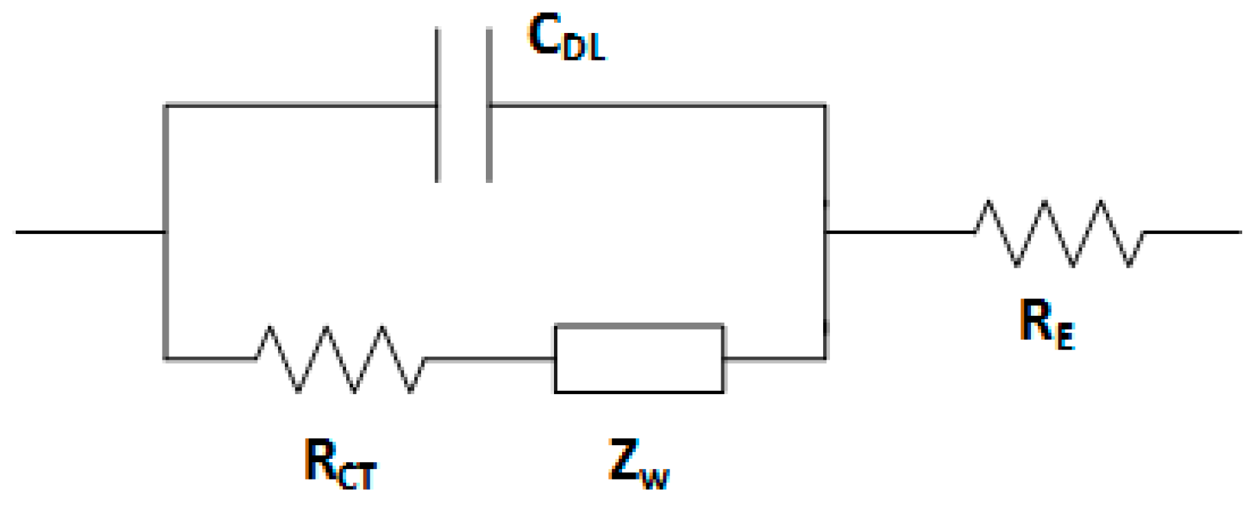
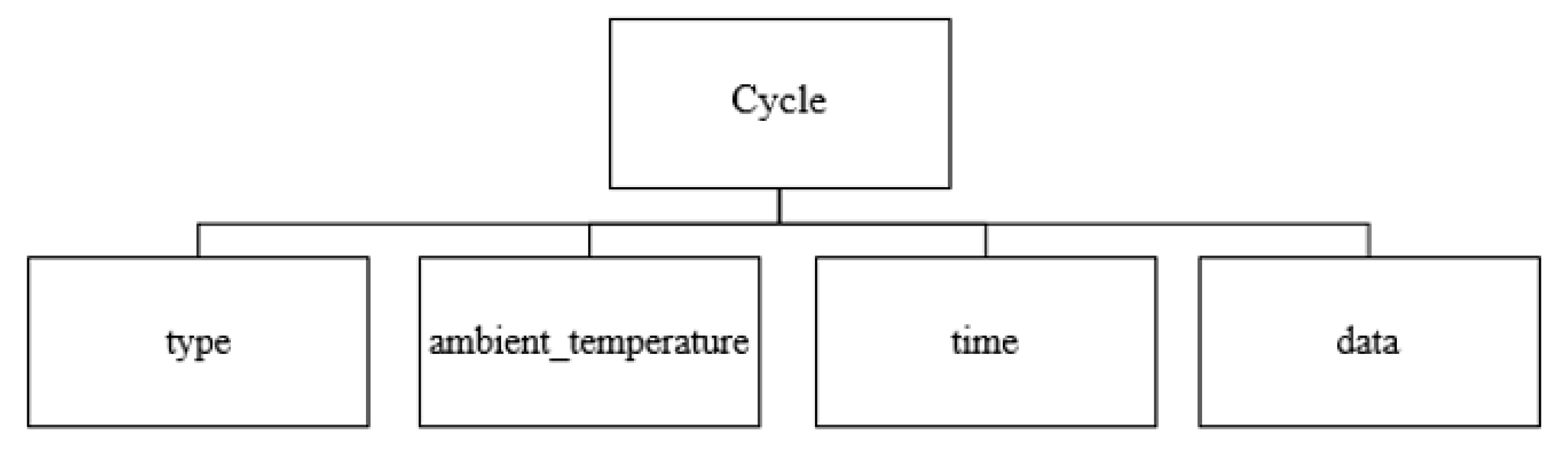
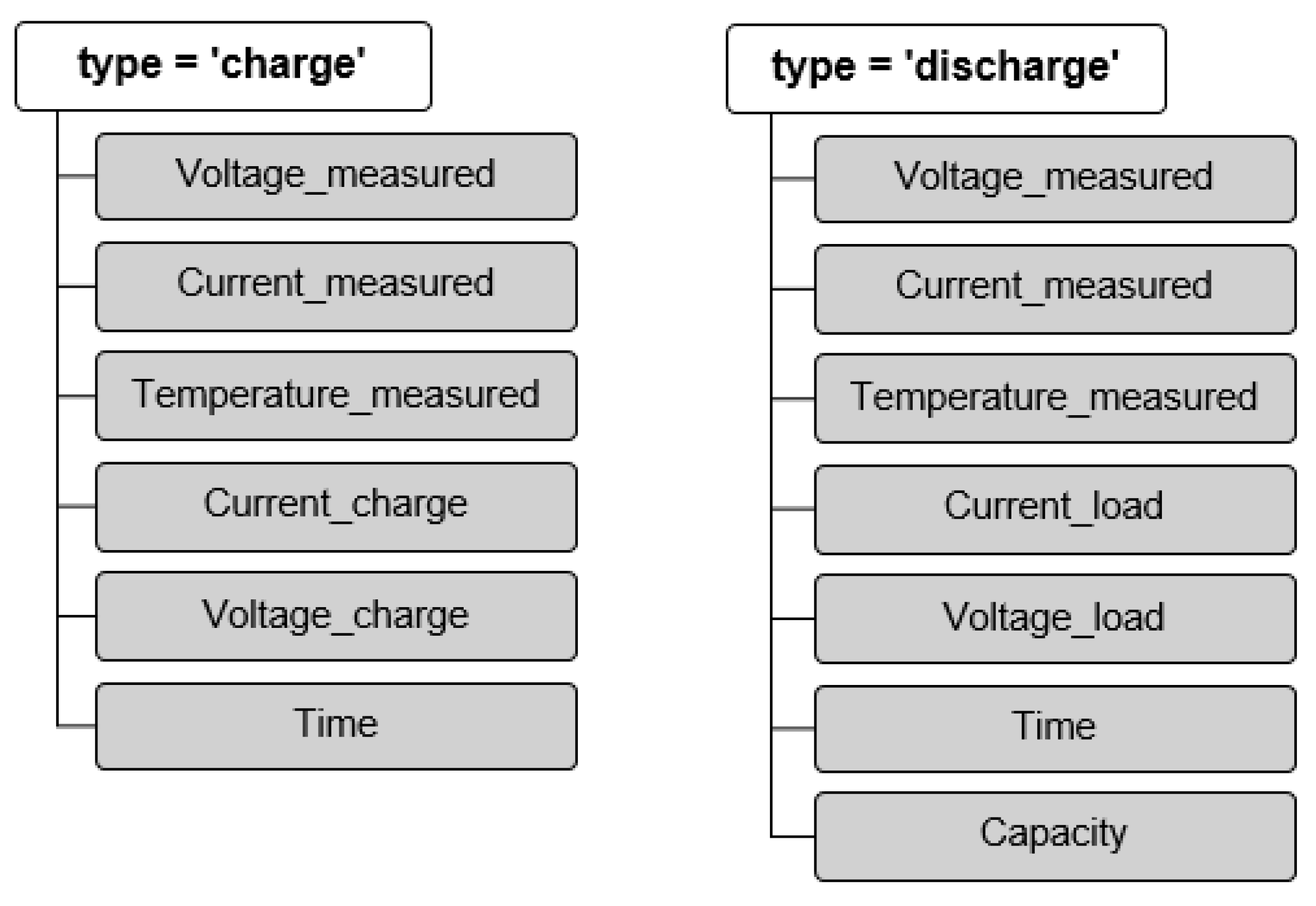
3.1. Battery Modeling and Feature Extraction

The Randle’s circuit model (Figure 1) is used in the EOD and EOL prediction. The main reason for using this model is because it uses internal processes such as voltage drop due to the internal resistance of the battery and the polarization effects. The EOD and EOL models developed later were originally proposed by Saha and Goebel [14], who carried out the feature extraction using RVM algorithms. In this research, the effects of battery aging and different loading profiles are added to enhance their model.

3.2. Battery Capacity Fade Model

The Coulombic Efficiency factor (${\eta }_C$) models the effect of battery capacitor fade with aging and cycling. This factor represents the amount of charge that can be extracted from a battery given the charged capacity. The reduction of the battery capacitor with aging is modelled as:

$$C_k={\left({\eta }_C\right)}^k·C_0,$$

(2)

where k represents the cycle and $C_0$ is the initial capacitance of the battery. Through experimental testing, a typical value for ${\eta }_C$ = 0.9987. However, the capacity usually increases when the battery is allowed to rest between cycles. Therefore, a battery ‘self-recharge during rest’ factor was introduced by Saha and Goebel [14]. The battery EOL model is now expressed as:

$$C_k={\left({\eta }_C\right)}^k·C_0+{\beta }_1·\exp \left(\frac{-{\beta }_2}{\Delta t_k}\right),$$

(3)

where $\Delta t_k$ is the resting time between $k$ and $k-1$ cycles and ${\beta }_1$ and ${\beta }_2$ are the model parameters to be determined and tracked using the particle filter algorithm.

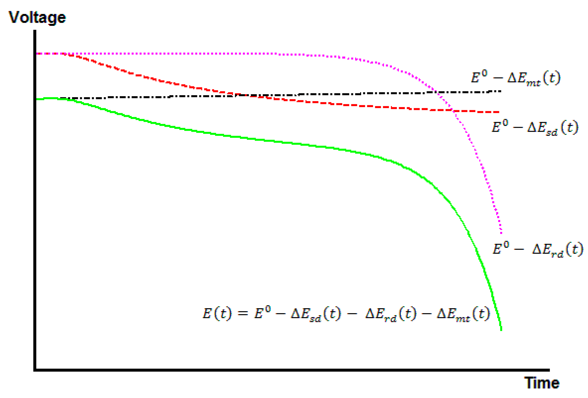
3.3. Battery Discharge Model

The Randle’s circuit model is used to develop the End of Discharge (EOD) model. The voltage drop is expressed as:

$$E=E_0-I·\left(R_E+R_{CT}+Z_w\right),$$

(4)

where $E^0$ is the theoretical open circuit voltage; $I$ is the current flowing out of the battery; and $R_E$, $R_{CT}$ and $Z_w$ are the electrolyte resistance, charge transfer resistance, and Warburg impedance, respectively.

This expression can also be rewritten to include the internal resistances of the battery:

$$E\left(t\right)=E^0-\Delta E_{sd}\left(t\right)-\Delta E_{rd}\left(t\right)-\Delta E_{mt}\left(t\right),$$

(5)

where $\Delta E_{sd}$ is the voltage loss due to battery shelf discharge, $\Delta E_{rd}$ is the drop caused by the cell reactant depletion, and $\Delta E_{mt}$ represents the drop due to internal resistance to mass transfer.

The individual terms of Equation (4) are expressed as:

$$\Delta E_{sd}\left(t\right)={\alpha }_1·\exp (\frac{-{\alpha }_2}{t})$$

(6)

$$\Delta E_{rd}\left(t\right)={\alpha }_3·\exp \left({\alpha }_4·t\right)$$

(7)

$$\Delta E_{mt}\left(t\right)=\Delta E_{init}-{\alpha }_5·t.$$

(8)

Model parameters ${\alpha }_1,{\alpha }_2,{\alpha }_3,{\alpha }_4,{\alpha }_5$ are to be calculated and $\Delta E_{init}$ is the voltage drop as the current, $I$, passes through the internal resistance, $R_E$, at the start of the discharge cycle. This is calculated by $\Delta E_{init}=I\times R_E$. The effect of each term and the whole EOD model is shown in Figure 2. It can be observed that from the three components given in Equations (6)–(8), the cell reactant depletion ($\Delta E_{rd}$) is the main term when determining the EOD. For this reason, ${\alpha }_3$ and ${\alpha }_4$ will be the most important model parameters affecting the EOD prediction.

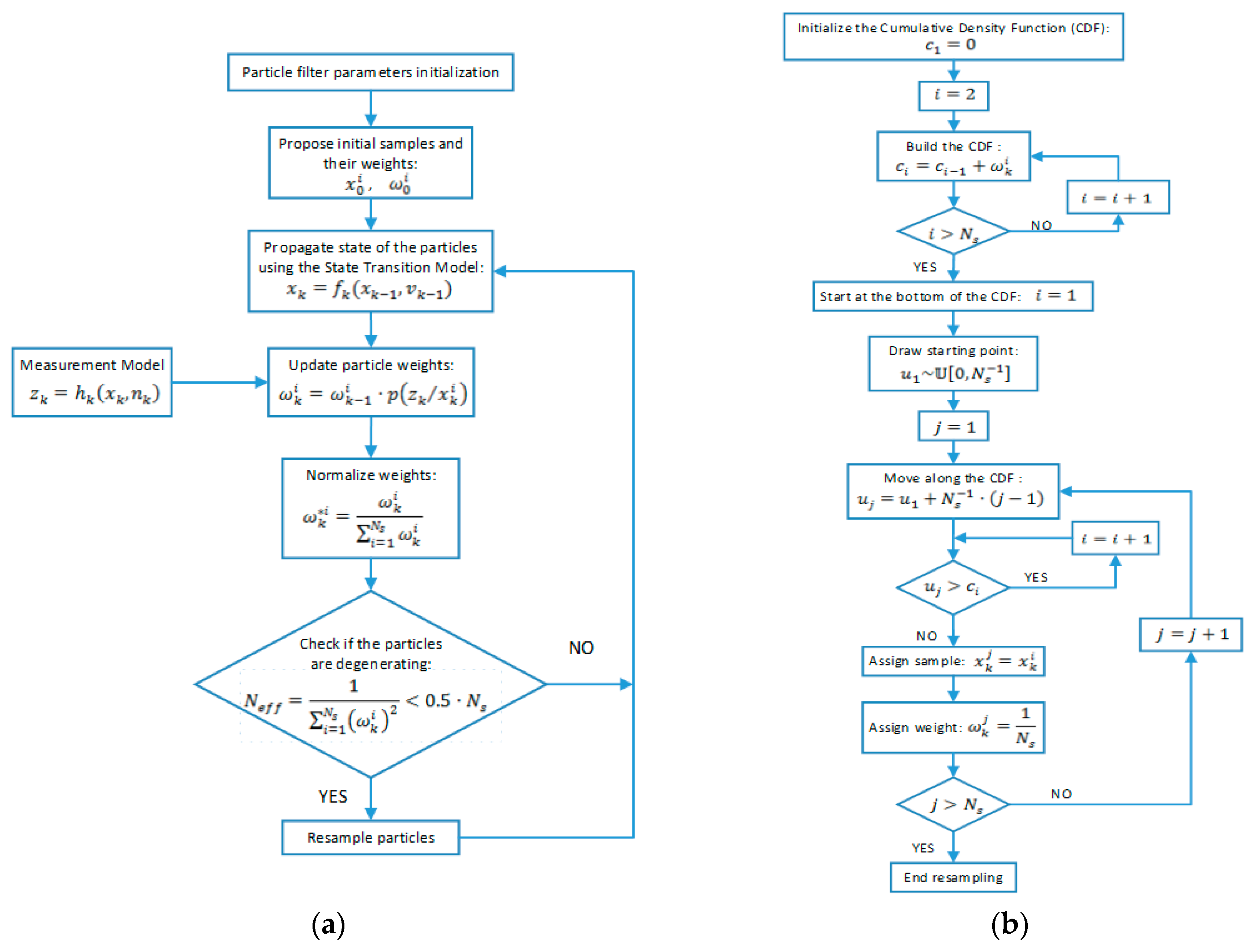
3.4. Particle Filter Framework

As Kalman filters, Particle Filters (PFs) are an excellent tool to track the state of a system. The main reason for using PFs instead of Extended Kalman filters is that the latter usually need a high computational effort to obtain an exact solution, whereas the former usually find quite a good approximate solution with less computational effort [27].

The particle filtering technique, also called bootstrap filtering or survival of the fittest, is a sequential Monte Carlo (MC) method that is described in detail in [28]. It represents the predicted state of the system using a group of random particles and their associated weights. This is shown in Equation (9):

$$p\left(x_{0:k}/z_{1:k}\right)\approx {{\displaystyle \sum }}_{i=1}^{N_s}{\omega }_k^i·\delta \left(x_{0:k}-x_{0:k}^i\right),$$

(9)

where $\{x_{0:k}^i,i=0,\dots ,N_s\}$ are the set of $N_s$ particles or samples up to time step $k$, and $\{{\omega }_k^i,i=1,\dots ,N_s\}$ are the associated weights for the particles at time step $k$. A normalization of the weights is required at every time step to ensure that ${{\displaystyle \sum }}_i{\omega }_k^i=1$.

The state of the system is propagated using the system model, and the weights are updated for every time step when new measurements are available. The quality of the algorithm depends on the choice of the weight update function. There are several ways to update the weights:

• Sequential importance sampling: when an importance density function $q(·)$ is available, the weights can be updated using:

  $${\omega }_k^i\propto {\omega }_{k-1}^i·\frac{p\left(z_k/x_k^i\right)·p\left(x_k^i/x_{k-1}^i\right)}{q\left(x_k^i/x_{k-1}^i,z_k\right)}.$$

  (10)
• When the importance density sampling function is chosen so that it reduces the variance of the weights:

  $${\omega }_k^i\propto {\omega }_{k-1}^i·p\left(z_k/x_{k-1}^i\right).$$

  (11)
• Occasionally, the importance density sampling function is chosen to be the PDF of the state based only on the previous state ($q\left(x_k^i/x_{k-1}^i,z_k\right)=p\left(x_k/x_{k-1}^i\right)$). The weight update function is then:

  $${\omega }_k^i\propto {\omega }_{k-1}^i·p\left(z_k/x_k^i\right).$$

  (12)

An important issue with the particle filter algorithm is the degeneracy problem. This occurs when, after several iterations, a few particles have a high weight, making the other samples negligible. The degeneracy problem is usually evaluated using the effective sample size $N_{eff}$, which is calculated using:

$$N_{eff}\approx \frac{1}{{{\displaystyle \sum }}_{i=1}^{N_s}{\left({\omega }_k^i\right)}^2}.$$

(13)

When the effective sample size falls below a chosen threshold, a resampling technique is required in order to ensure the efficiency of the algorithm. The aim of resampling is to eliminate particles with low weights and focus on the particles with higher weights. The resampling strategy used in [28] is adopted. The particle filter strategy is shown in Figure 3a and the resampling strategy is displayed in Figure 3b.

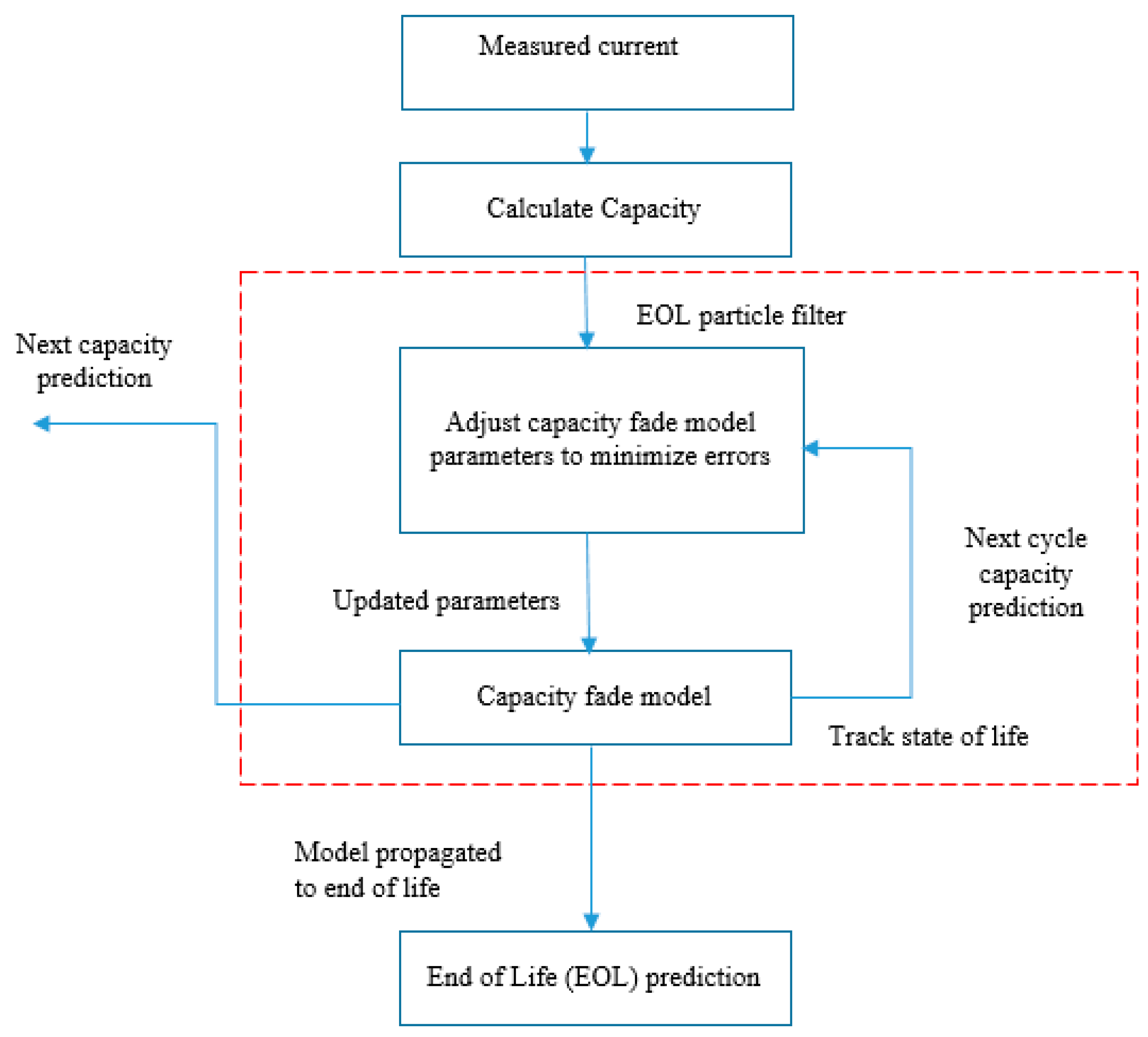
3.5. End of Life (EOL) Prediction Model

The EOL prediction methodology is shown in Figure 4 and predicts the RUL of the battery through the integration of sensor measurements, a particle filter, and other calculations. The battery degradation is mainly affected by the capacity fade. The capacity must be evaluated using parameters monitored by a Battery Management System (BMS) since there is no mechanism to measure the capacity of a cell. These parameters are the cell voltage, input or output current, and temperature. Only the output current is required for estimating the cell capacity, which is calculated using the Coulomb counting method as in Equation (14):

$$\mathrm{C}={\displaystyle \int }\mathrm{I}\mathrm{dt}.$$

(14)

Therefore, the cell output current must be integrated during a full discharge cycle. The important point is that the battery is not always fully charged or discharged. Therefore, tables with available test data and other estimation algorithms are required to accurately predict the battery’s State of Health (SOH). The particle filter is another important factor in the EOL prediction model. The particle filter consists of two models: state transition and the measurement model. The state transition model is expressed as:

$${\beta }_{1,k+1}={\beta }_{1,k}+{\phi }_{1,k}$$

(15)

$${\beta }_{2,k+1}={\beta }_{2,k}+{\phi }_{2,k}$$

(16)

$$C_{k+1}={\eta }_c·C_k+{\beta }_{1,k}·\exp \left(\frac{-{\beta }_{2,k}}{\Delta t_k}\right)+{\phi }_k,$$

(17)

where ${\phi }_{1,k}$, ${\phi }_{2,k}$, and ${\phi }_k$ denote the zero-mean Gaussian noise terms. The measurement model is expressed by [14]:

$${\tilde{C}}_k=C_k+{\psi }_k,$$

(18)

where ${\psi }_k$ characterizes the measurement noise, again modeled as zero-mean Gaussian noise, and ${\tilde{C}}_k$ denotes the measured capacity. The particle filter monitors the state of the battery using these two models by producing accurate predictions every time a new measurement is present. The algorithms propagate the state of the system until the EOL capacity threshold, when an EOL prediction is required. This propagation means estimating the evolution through the state transition model using the latest update of parameters ${\beta }_1,{\beta }_2$, and $\Delta t_k$. The EOL prediction for this study was chosen to be 80% of the battery nominal capacity (i.e., 1.6 Ahr for a cell of 2 Ahr nominal capacity) since it is the value utilized by the industry to reject a faulty battery. The effects of battery aging and different loading profiles are added to enhance their model.

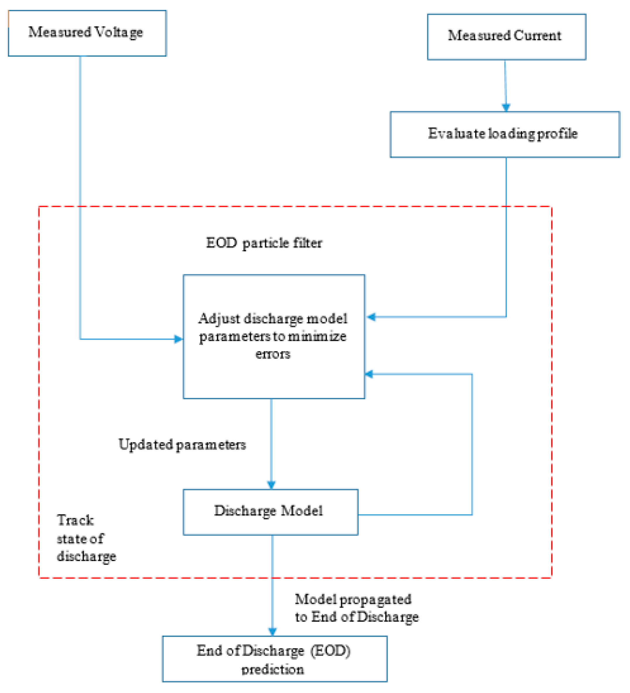
3.6. Enhanced End of Discharge (EOD) Prediction Model

The EOD prediction methodology is shown in Figure 5. The model includes measurements from the sensors, the particle filter to track the state of discharge and prediction, and other algorithms that adapt the model for different loading profiles. Both voltage and current are required for the EOD prediction. The state of charge (SOC) is reflected by the voltage and the loading profile is evaluated by the measurement of the current. Every time a new current measurement is present, the battery state of charge is updated to comprise the effects of the charge that has been already extracted from the battery. This is achieved using Equation (19):

$$SO{C}_{i+1}\approx SO{C}_i+\frac{I_i·T_S}{C},$$

(19)

where $T_S$ represents the sampling period, $I_i$ is the measured current of the battery, and $C$ is the current capacity of the battery for that discharge cycle, evaluated by the EOL particle filter. The particle filter is able to track the state of the cell during discharge once the loading profile is evaluated. The state transition and measurement models are described in Equations (20)–(25). The state transition model is based on work carried out by Saha and Goebel [14], but includes some modifications, given by:

$${\alpha }_{1,i+1}={\alpha }_{1,i}+v_{1,i}$$

(20)

$${\alpha }_{2,i+1}={\alpha }_{2,i}+v_{2,i}$$

(21)

$${\alpha }_{3,i+1}={\alpha }_{3,i}+v_{3,i}$$

(22)

$${\alpha }_{4,i+1}=a·\frac{\left(1-SO{C}_i\right)}{t_i}+v_{4,i}$$

(23)

$${\alpha }_{5,i+1}={\alpha }_{5,i}+v_{5,i}$$

(24)

$$E_{i+1}=E_i-\frac{{\alpha }_{1,i}·{\alpha }_{2,i}·\exp \left(\frac{-{\alpha }_2}{t_i}\right)/t_i^2-{\alpha }_{3,i}·{\alpha }_{4,i}·\exp \left({\alpha }_{4,i}·t_i\right)-{\alpha }_{5,i}}{f_s}+v_{6,i},$$

(25)

where $v_{1,i}$, $v_{2,i}$, $v_{3,i}$, $v_{4,i}$, $v_{5,i}$, and $v_{6,i}$ are independent zero-mean Gaussian noise terms; $a$ is a constant adjusted when tuning the algorithm; $t_i$ is the current time; and $f_s$ is the sampling frequency. The novelty of this study when compared to the model proposed by Saha and Goebel [14] is the method of calculating ${\alpha }_4$. Determination of ${\alpha }_4$ according to Saha and Goebel’s method is shown by Equation (21). In their model, the values were initialized knowing the loading profile and capacity in advance. The calculation in Equation (23) for ${\alpha }_4$ allows the parameters to adapt to different loads. This proposed modification of ${\alpha }_4$ also works when the capacity has faded away, causing a reduction in the EOD time.

$${\alpha }_{4,i+1}={\alpha }_{4,i}+v_{4,i}$$

(26)

The measurement model is expressed as:

$$z_i=E_i+n_i,$$

(27)

where $n_i$ is the measurement noise, modeled as zero-mean Gaussian noise; and $z_i$ is the measured voltage at time $t_i$. The particle filter tracks the state of charge of the battery by using these two models, giving accurate predictions of the state of the next step every time a new measurement is present. The particle filter propagates the current state of the battery until it reaches the EOD voltage threshold when the user requires a prediction of the remaining time for the discharge of the battery. This threshold can be adjusted in order to maximize the discharge time by setting a low EOD voltage threshold such as 2 V or reduce aging due to overcharging by setting a moderate value such as 2.7 V. The last update of the variables ${\alpha }_1,{\alpha }_2,{\alpha }_3,{\alpha }_5$ is maintained and the parameter ${\alpha }_4$ recalculated by assuming that the loading profile used by the application remains the same until the end of discharge in order to propagate the current state of the battery. This is achieved using Equation (28):

$$SO{C}_{i+1}\approx SO{C}_i-\frac{\left(1-SO{C}_i\right)·T_S}{t_i},$$

(28)

where the sampling period $T_S$ is used to update the time $t_i$. Similarly, with the EOL model, the EOD model does not output one value for the end of discharge time of the cell. Instead, a probability density function is calculated for the possible time interval when the charge of the cell is estimated to end.

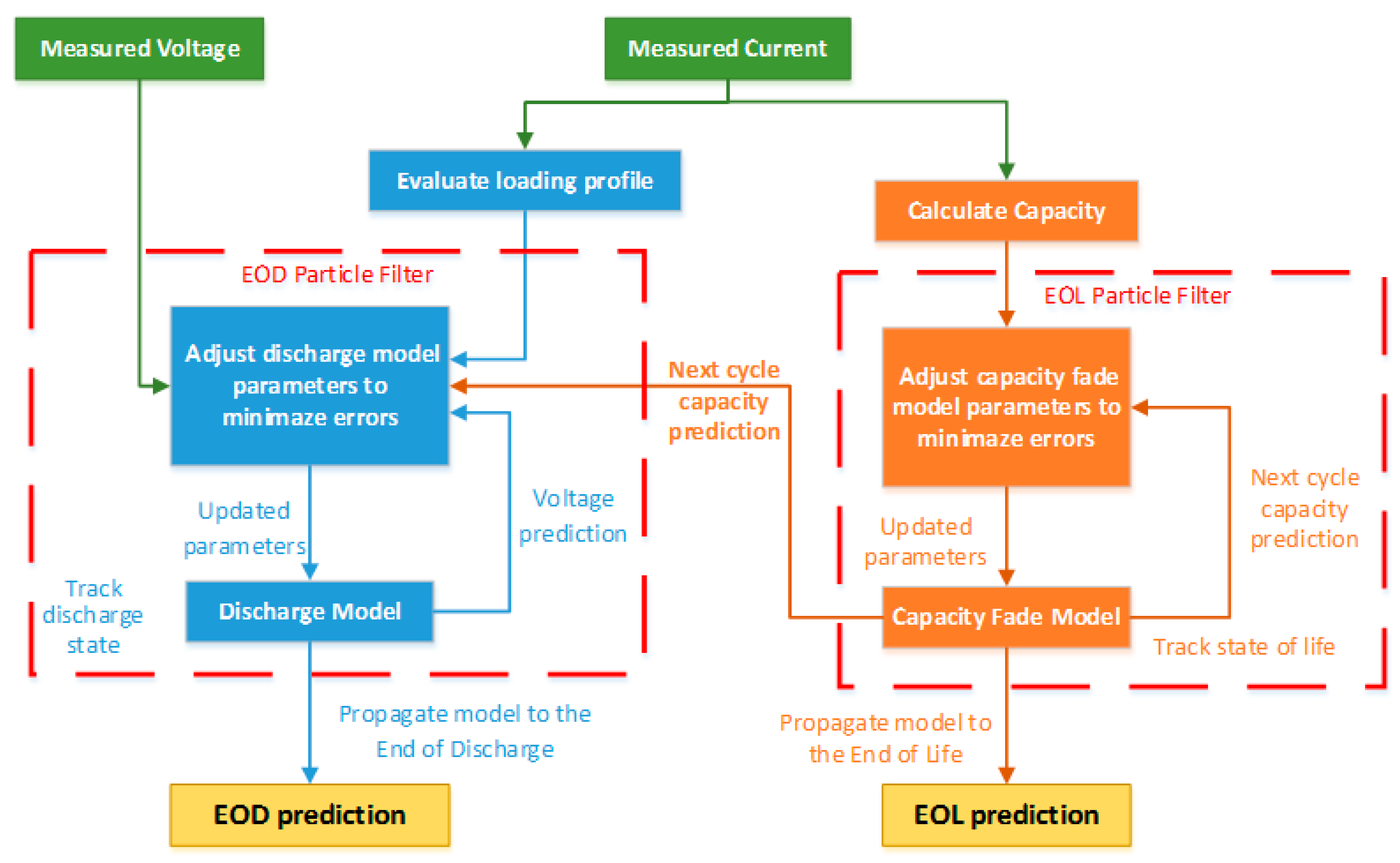
3.7. Diagnostic and Prognostic Framework

An overview of the diagnostic and prognostic framework is shown in Figure 6. The capacity for each discharge cycle is updated using both the EOD and EOL prediction models. Therefore, the EOD prediction model is more accurate, giving a battery system operator more information on when to replace a battery.

4. Simulation

This section discusses the methods and resources used in the EOL and EOD prediction. MATLAB/Simulink was chosen to implement these models along with online data from lithium ion cells. Refer supplementary material for EOD and EOL prediction codes.

Battery Specifications and Loading Conditions

The battery dataset for the analysis was downloaded from the NASA Ames Prognostics Data Repository. The dataset consists of 34 commercially available second-generation 18650-size lithium ion rechargeable cells of 2 Ahr nominal capacity. These batteries were cycled using different environmental conditions and loading profiles. The voltage, current, and temperature measurements were recorded during charging and discharging of the batteries. An environmental chamber was used to expose the batteries to different temperatures while cycling (4, 24 and 44 °C). Fixed and variable loading profiles of 1, 2 and 4 A were used and several End of Discharge (EOD) voltages were used (2, 2.2, 2.5 and 2.7 V) in order to get sufficient data on battery behavior under different operating conditions. One important factor to note is that the batteries were mostly tested in sets of four and not all of them were cycled until the capacity has faded 20% of its nominal value. Therefore, certain datasets were unsuitable for the EOL prediction model. The charging protocol used for the cells was Constant Current of 1.5 A until the cell voltage reached 4.2 V and then Constant Voltage until the current dropped under 20 Ma. The recorded data were stored in .MAT files consisting of all cycling measurements for a given cell, which are stored in an array of ‘Cycle’ structures. This data structure is shown in Figure 7. Each cycle structure consists of measurements from one of the three types: charge, discharge, and impedance. The Time array consists of the sampling times, while the other field contains current and voltage measurements (Figure 8). The Capacity field was evaluated by integrating the current over time until the battery voltage reaches 2.7 V.

5. Results and Discussion

This section of the paper presents the results and discussions of the End of Life (EOL) and End of Discharge (EOD) predictions.

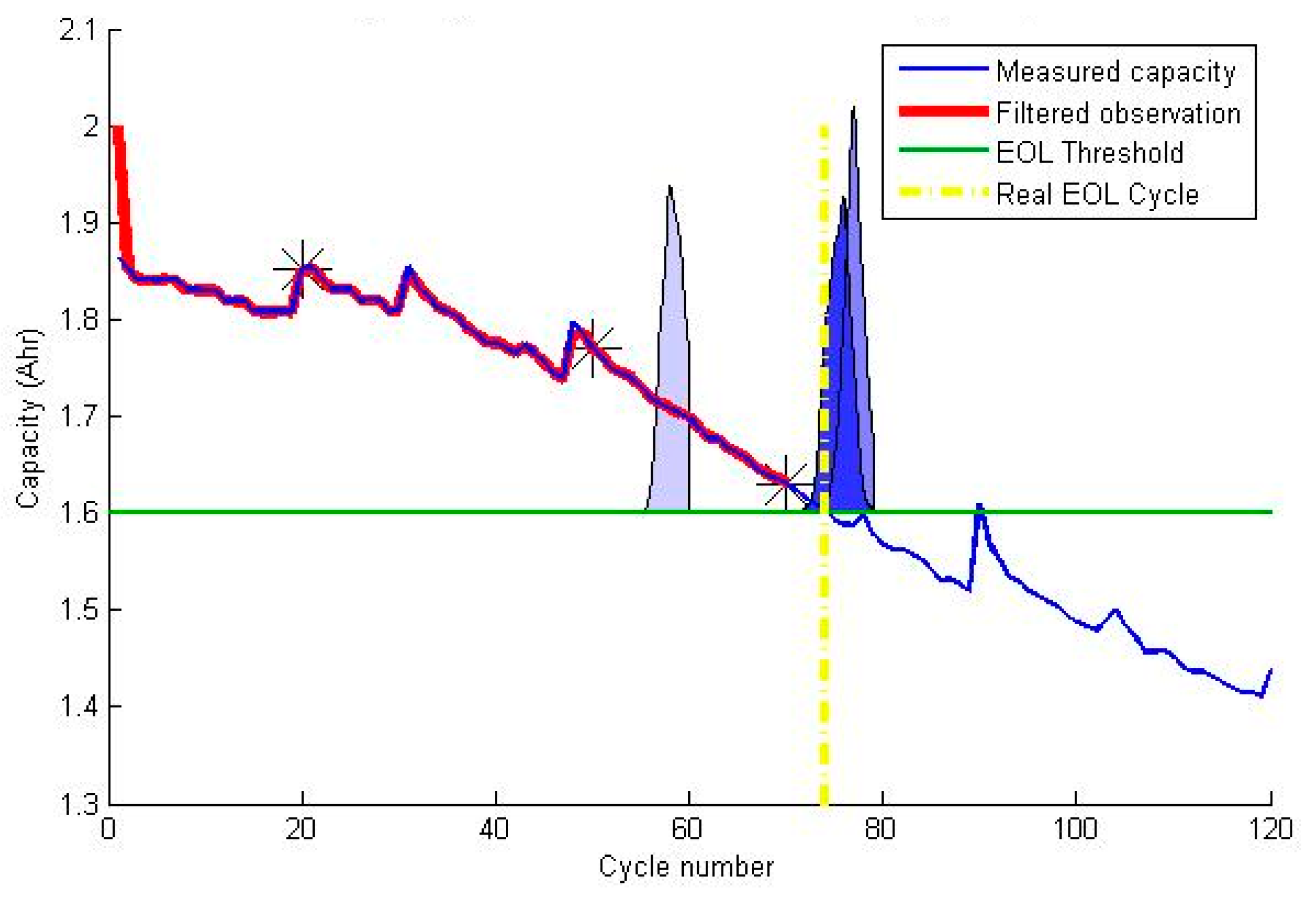
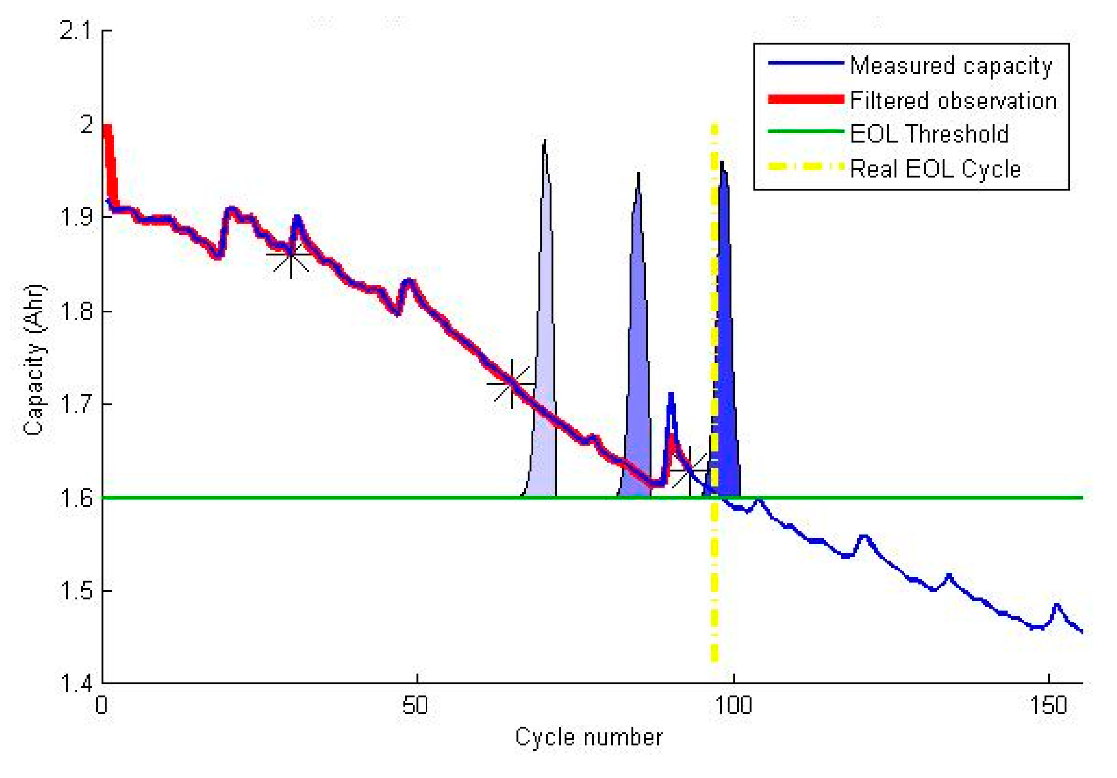
5.1. End of Life (EOL) Prediction

The accuracy of the EOL model was tested using the model and equations explained in Section 3.2. The value for ${\eta }_C=0.9987$ was chosen. The number of particles used was 400, which results in a good accuracy, sustaining a sensible computer workload. The particles were normalized using random numbers through a normal distribution with mean $0.5,3\times {10}^5$ and 1.8 for ${\beta }_1,{\beta }_2$ and $C$ respectively. The algorithm tracks the state of the system by modifying these parameters. The state parameters evolve with time by means of the noise added in the state transition model by the terms ${\phi }_{1,k},{\phi }_{1,k}$ and ${\phi }_k$. The following paragraphs and figures show the different tests of the framework for EOL prediction.

5.1.1. EOL Prediction (First Test)

The first test involved a cell cycled at 24 °C using a 2 A discharge current until the voltage reached the EOD voltage of 2.7 V, corresponding to the cell B0005 of the dataset. The blue line in Figure 9 depicts the cell capacity of each cycle, the red line is the filtered observation from the particle filter, the green line is the EOL threshold of 20% capacity loss, and the dotted vertical yellow line denotes the real EOL cycle, which is cycle 76 in this case. The predictions were performed at cycles 20, 50, and 70 and a scaled PDF of the possible EOL cycles was obtained. The lightest blue PDF denotes the earliest prediction, whereas the darker one is the most recent prediction. It is proven that the prediction is more accurate as the EOL cycle approaches; this prediction error will be analyzed in the later sections of this paper.

5.1.2. EOL Prediction (Second Test)

Figure 10 shows a test for cell B0007, which was also cycled with a 2 A discharge current and at 24 °C. However, the EOD voltage for this cell is 2.2 V. Therefore, this cell was cycled with a higher depth of discharge.

5.1.3. EOL Prediction (Third Test)

Figure 11 depicts the test for cell B0030, which was cycled with a 4 A discharge current and at 43 °C until the voltage reached 2.2 V for each discharge cycle. The capacity fade increases for higher demanding operating conditions (higher discharge current and ambient temperature), which would result in a smaller EOL cycle. However, the initial capacity is lower than the algorithm initialization value; yet the framework and the particle filter converge, resulting in predictions that become increasingly accurate with time.

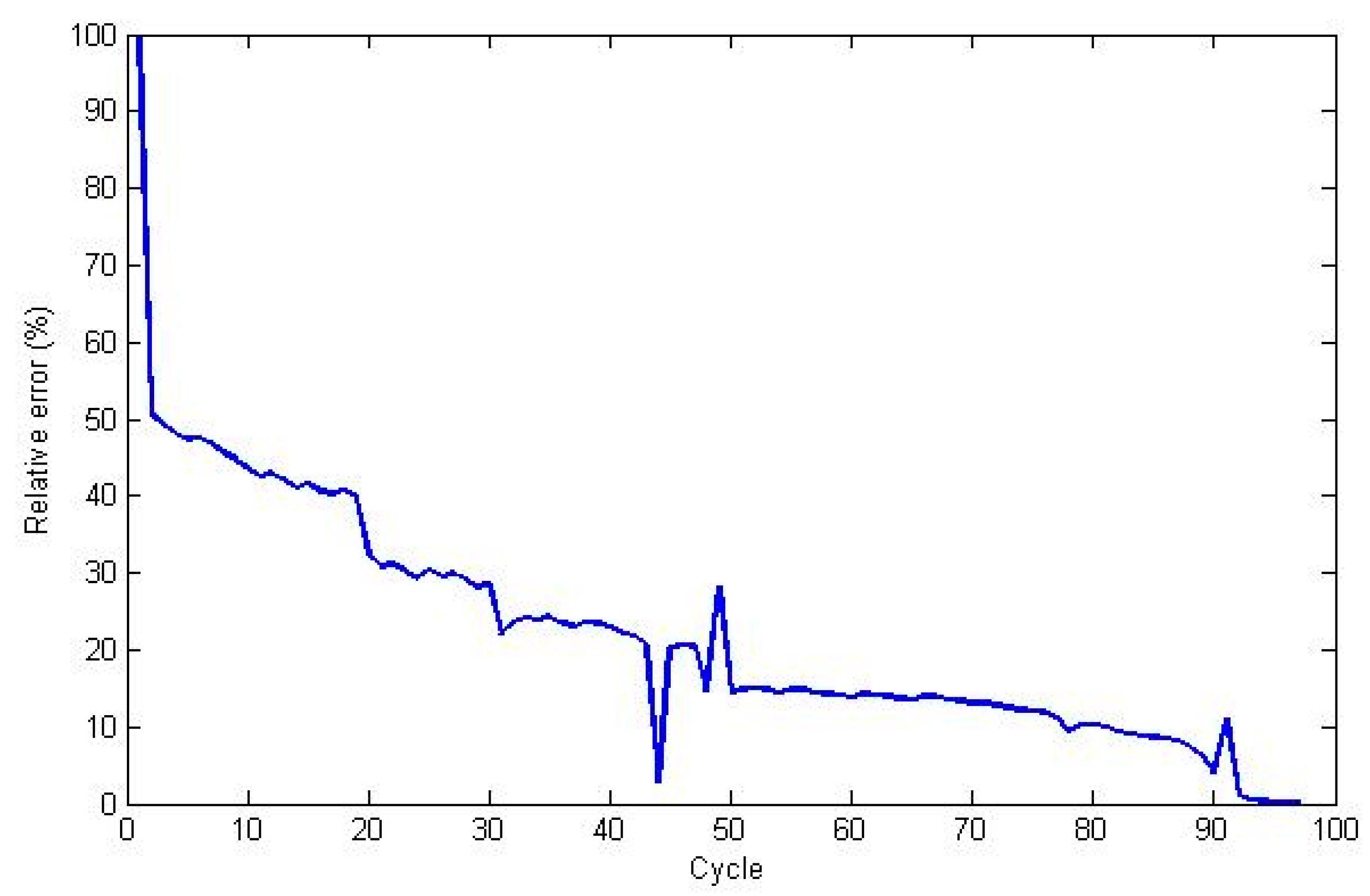
5.1.4. EOL Prediction Error

In order to evaluate the evolution of the EOL prediction error with time, another test was performed. This was achieved by propagating the state for every cycle until the EOL. The relative error is evaluated using Equation (29) and an example is shown in Figure 12:

$$Relativeerror=\frac{\left|EO{L}_{Predicted}-EO{L}_{Real}\right|}{EO{L}_{Real}}.$$

(29)

In order to compute the EOL prediction, another expression was used instead of using the probability density function. This expression is:

$$EO{L}_{Predicted}={{\displaystyle \sum }}_{i=1}^{N_s}{\omega }_k^i·EO{L}_{Predicted,k}^i.$$

(30)

Figure 12 shows the EOL prediction error test for cell B0007. It is shown that the accuracy is at least 20%, which is fewer than 10 cycles once the algorithm has converged.

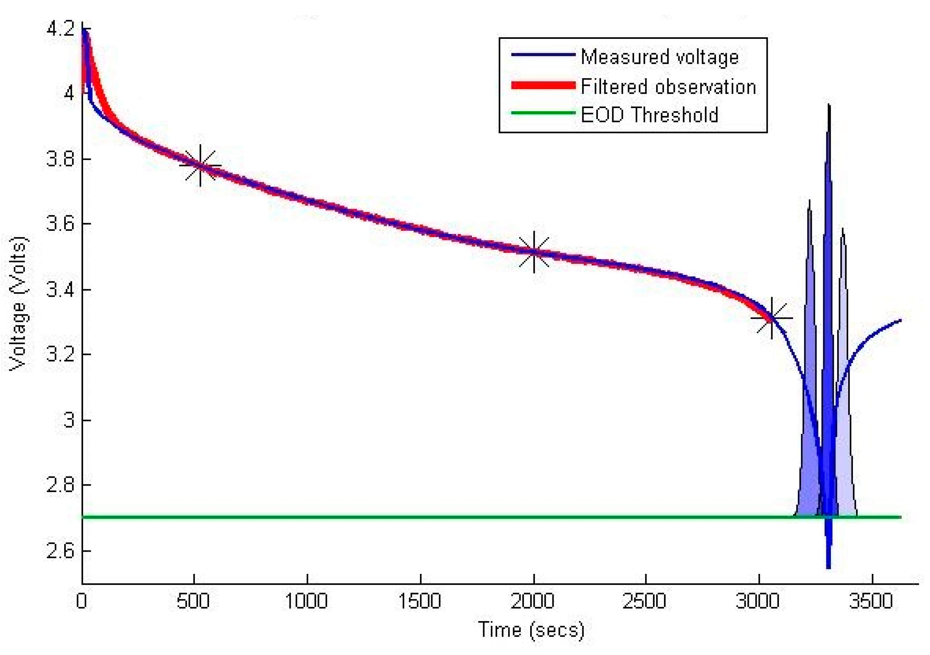
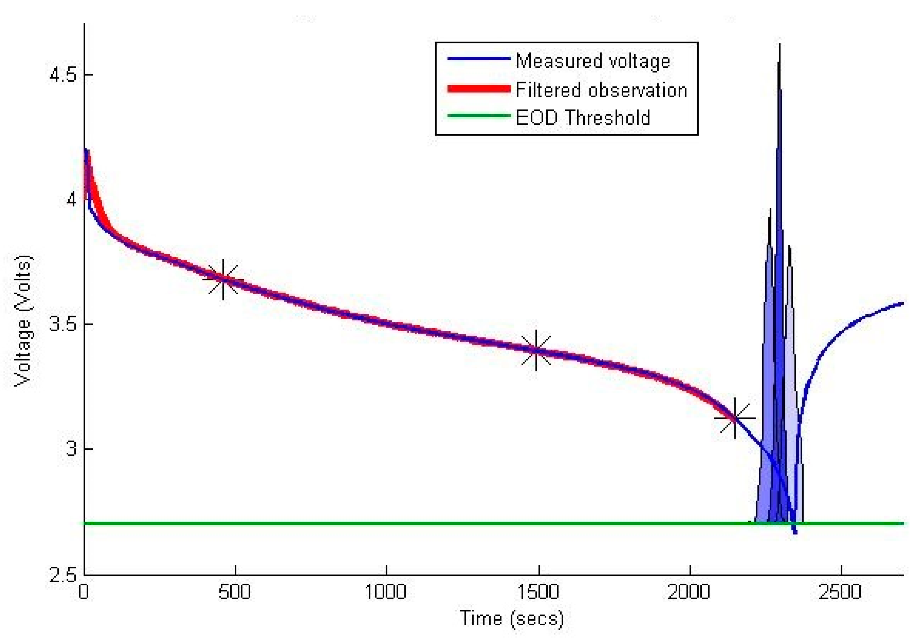
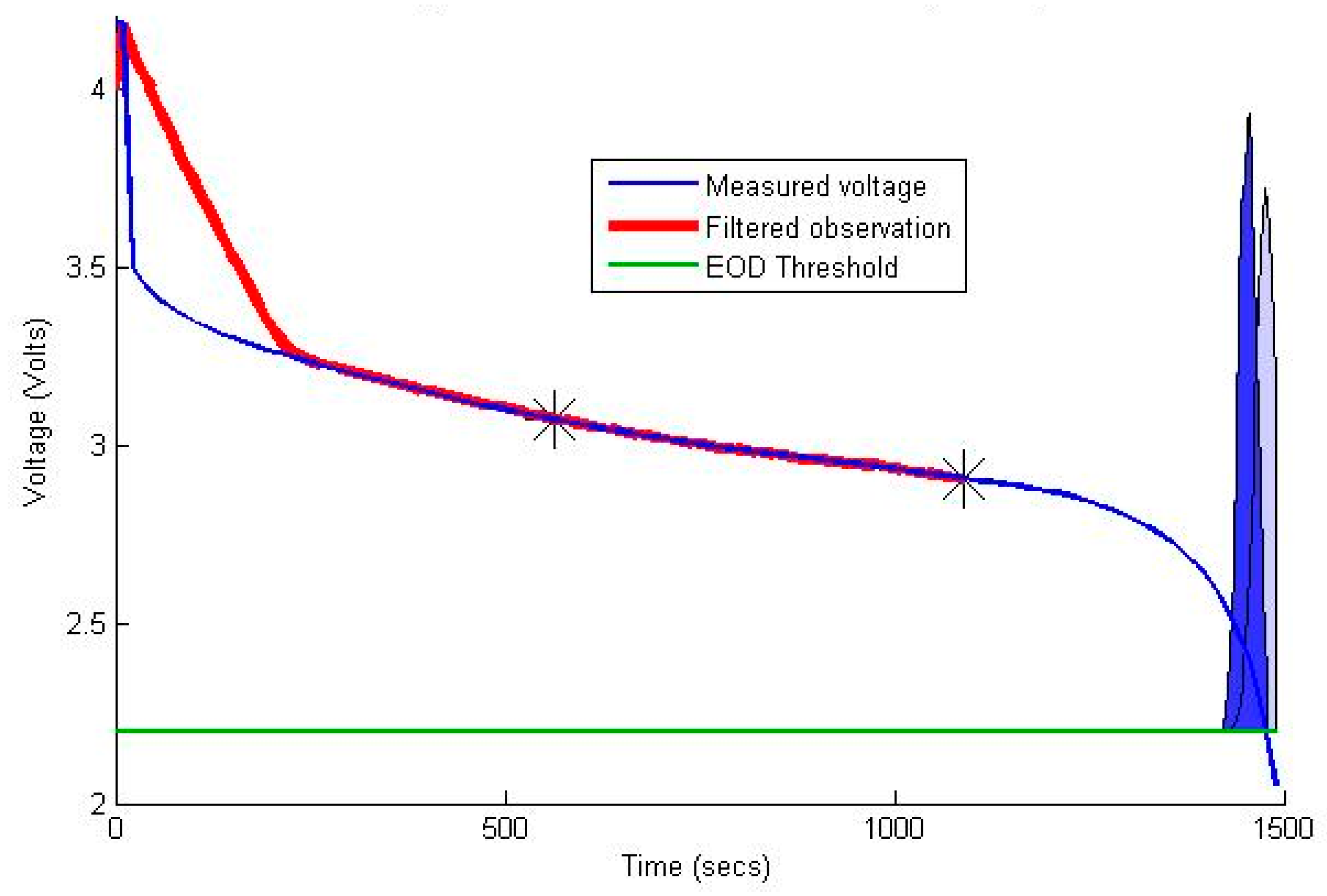
5.2. End of Discharge (EOD) Prediction

The EOD prediction was done with the equations given in earlier sections. Similarly to the EOL prediction, 400 particles were used for the particle filter to get a good accuracy and maintain a reasonable computer workload. These particles were initialized using random numbers from a normal distribution, with mean 0.6, 900, $2.2\times {10}^{-5},3.8\times {10}^{-3},1\times {10}^{-7}$, and 4 for ${\alpha }_{1,0},{\alpha }_{2,0},{\alpha }_{3,0},{\alpha }_{4,0},{\alpha }_{5,0}$, and $E_0$, respectively (the six components of the particle filter state vector in Equations (20)–(25) where $\alpha =10.8$). The algorithms track the state of the system by adjusting these parameters so the predicted voltage approaches the real measurement. The state parameters evolve with time by means of the noise added in the state transition model. Several tests are carried out for the EOD prediction framework.

5.2.1. EOD Prediction (First Test)

This test was carried out for a cell cycled at 24 °C using a 2 A discharge current until the voltage reached the EOD voltage of 2.7 V, corresponding to cell B0005 of the dataset. The EOD prediction was tested for two cycles of the dataset, one of the earliest (discharge cycle 5) and one of the latest (discharge cycle 160). The main reason for doing this was to show that the algorithms perform well when the EOD time is reduced due to the capacity fade with cycling. Figure 13 shows the results for the discharge cycle 5, following the same logic as for EOD: the measured voltage is the blue line, the filtered observations from the particle filter are the thick red line, and the EOD threshold is denoted by the green line. The real EOD time is evaluated when the measured voltage goes below the EOD voltage threshold. Once again, three predictions were done at three times while discharging. The state of the particles was propagated for each of them, obtaining the scaled probability density functions of the possible EOD times. The earliest prediction is denoted by the lightest blue PDF and the darker one depicts the most recent one. The prediction becomes more accurate as the EOD time approaches. The results are depicted in Figure 13.

5.2.2. EOD Prediction (Second Test)

Figure 14 shows the test for the discharge cycle 160. The results show that the accuracy of the prediction remains almost the same, while the EOD time has reduced from around 3300 to 2400 s.

5.2.3. EOD Prediction (Third Test)

The third test involved cell B0038, which was cycled at different ambient temperatures of 24 and 44 °C during its lifetime using different discharge currents of 1, 2 and 4 A. The EOD voltage for this cell was 2.2 V and the last discharge cycle with a discharge current of 4 A was selected. The framework proved to work for different environmental and loading conditions for this test. The results for the two EOD predictions carried out are shown in Figure 15. Two EOD predictions were carried out and the results are shown in Figure 15. It can be seen that the algorithm needs some time to converge due to the initial voltage drop in the cell, but the predictions done around times 600 and 1100 show a quite accurate estimation of the EOD time.

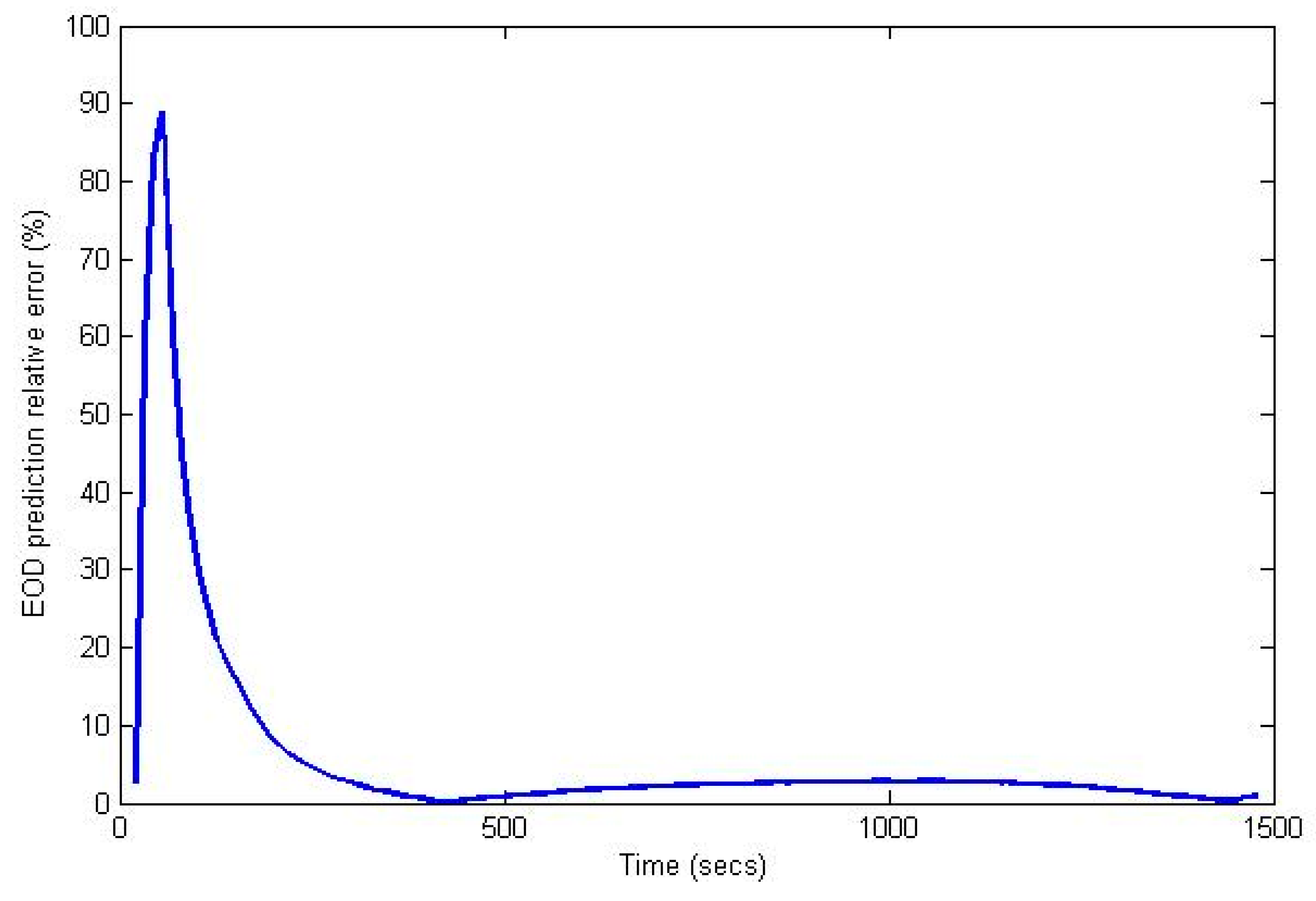
5.2.4. EOD Prediction Error

The error in the EOD prediction was evaluated to estimate the accuracy of the prediction. This was done by propagating the state until the EOD for every time step of the particle filter with the aim of estimating the evolution of the EOD prediction error with time. Equations are used for this task, similar to the EOL prediction.

$$EO{D}_{Predicted}={\displaystyle \sum }_{i=1}^{N_s}{\omega }_k^i·EO{D}_{Predicted,k}^i$$

(31)

$$Relativeerror=\frac{\left|EO{D}_{Predicted}-EO{D}_{Real}\right|}{EO{D}_{Real}}$$

(32)

Figure 16 shows the result for the last discharge cycle of cell B0038. The results proved that once the algorithms converge, the prediction is done with an error less than 10%. This implies that the prediction is quite practical.

6. Conclusions

The paper has focused on the prediction of the RUL for lithium ion batteries. The most common failure modes identified were capacity and power fade and battery shelf discharge. The various measurable parameters from a battery were defined before suggesting the prediction framework. A prognostic framework that involves End of Discharge (EOD) and End of Life (EOL) derived in this paper has been based on the discharge and capacity fade models developed by Saha et al. [14] Modifications were made and the effects of battery aging and different loading profiles were added. The particle filter was introduced and all the equations used for its implementation were devised. The EOL prediction model was then developed to describe how the reduction in capacity defines the cell cycle life. The EOD prediction model was modified to account for different loading profiles. Finally, the EOL and EOD prediction models were combined to study the effect of capacity fade in the reduction of the EOD time with cycling, thus giving a greater accuracy to the estimation. The proposed framework has been tested using MATLAB and real cell data available from NASA. Both the prediction models provided satisfactory results. The EOL cycle was predicted with a maximum error of 20% of the total cycle life and this error was reduced with the availability of more information. The EOD time prediction was more accurate with an error less than 10% once the algorithm converges.

References

1. Walker, E.; Rayman, S.; White, E.R. Comparison of a particle filter and other state estimation methods for prognostics of lithium-ion batteries. J. Power Sources 2015, 287, 1–12. [Google Scholar] [CrossRef]
2. Saha, B. NASA—Battery Prognostics; NASA: Washington, DC, USA, 2010. [Google Scholar]
3. Xi, Z.; Jing, R.; Lee, C. Diagnostics and Prognostics of Lithium-ion Batteries. In Proceedings of the ASME 2015 International Design Engineering Technical Conferences and Computers and Information in Engineering, Boston, MA, USA, 2–5 August 2015. [Google Scholar]
4. Jata, K.V.; Parthasarathy, T.A. Physics of Failure. In Proceedings of the 1st International Forum on Integrated System Health Engineering and Management in Aerospace, Napa, CA, USA, 7–10 November 2005. [Google Scholar]
5. Pecht, M. Prognostics and Health Management of Electronics; Wiley-Interscience: New York, NY, USA, 2008. [Google Scholar]
6. Xing, Y.; Ma, W.; Tsui, K. A Case Study on Battery Life Prediction Using Particle Filtering. In Proceedings of the 2012 Prognostics and System Health Management Conference, Beijing, China, 23–25 May 2012. [Google Scholar]
7. He, W.; Williard, N.; Osterman, M.; Pecht, M. Prognostics of lithium-ion batteries based on Dempster-Shafer theory and the Bayesian Monte Carlo method. J. Power Sources 2011, 196, 10314–10321. [Google Scholar] [CrossRef]
8. Pattipati, B.; Sankavaram, C.; Pattipati, K.R. System Identification and Estimation Framework for Pivotal Automotive Battery Management System Characteristics. IEEE Trans. Syst. Man Cybern. Part C Appl. Rev. 2011, 41, 869–884. [Google Scholar] [CrossRef]
9. An, D.; Choi, N.H.; Kim, N.H. Prognostics 101: A tutorial for particle filter-based prognostics algorithm using Matlab. Reliab. Eng. Syst. Saf. 2013, 115, 161–169. [Google Scholar] [CrossRef]
10. Gu, J.; Barker, D.; Pecht, M. Prognostics implementation of electronics under vibration loading. Microelectron. Reliab. 2007, 47, 1849–1856. [Google Scholar]
11. Pecht, M.; Dasgupta, A. Physics-of-failure: An approach to reliable product development. J. Inst. Environ. Sci. 1995, 38, 30–34. [Google Scholar]
12. Ye, M.; Guo, H.; Xiong, R.; Mu, H. An online model-based battery parameter and state estimation method using multi-scale dual adaptive particle filters. Energy Procedia 2017, 105, 4549–4554. [Google Scholar] [CrossRef]
13. Doucet, A.; Godsill, S.; Andrieu, C. On sequential Monte Carlo sampling methods for Bayesian filtering. Stat. Comput. 2000, 10, 197–208. [Google Scholar] [CrossRef]
14. Saha, B.; Goebel, K. Modelling Li-ion Battery Capacity Depletion in a Particle Filtering Framework. In Proceedings of the Annual Conference of the Prognostics and Health Management Society, San Diego, CA, USA, 27 September–1 October 2009. [Google Scholar]
15. Dalal, M.; Ma, J.; He, D. Lithium ion battery life prognostic health management system using particle filtering framework. Inst. Mech. Eng. Part O J. Risk Reliab. 2011, 225, 81–90. [Google Scholar] [CrossRef]
16. Daigle, M.; Saha, B.; Goebel, K. A Comparison of Filter-Based Approaches for Model-Based Prognostics. In Proceedings of the 2012 IEEE Aerospace Conference, Big Sky, MT, USA, 3–10 March 2012; pp. 1–10. [Google Scholar]
17. Wang, S.; Zhao, L.; Su, X.; Ma, P. Prognostics of Lithium-Ion batteries based on battery performance analysis and flexible support vector regression. Energies 2014, 7, 6492–6508. [Google Scholar] [CrossRef]
18. Tang, S.; Yu, C.; Wang, X.; Guo, X.; Si, X. Remaining useful life prediction of lithium ion batteries based on the wiener process with measurement error. Energies 2014, 7, 520–547. [Google Scholar] [CrossRef]
19. Qin, T.; Zeng, S.; Guo, J.; Skaf, Z. A rest time-based prognostic framework for state of health estimation of lithium-ion batteries with regeneration phenomena. Energies 2016, 9, 896. [Google Scholar] [CrossRef]
20. Huang, Q.; Shen, Y.; Huang, Y.; Zhang, L.; Zhang, J. Impedance characteristics and diagnosis of automotive lithium-ion batteries at 7.5% to 93% state of charge. Electrochim. Acta 2016, 219, 751–765. [Google Scholar] [CrossRef]
21. Sood, B.; Severn, L.; Osterman, M.; Pecht, M.; Bougaev, A.; McElfresh, D. Lithium-ion battery degradation mechanisms and failure analysis methodology. In Proceedings of the 38th International Symposium for Testing and Failure Analysis, Phoenix, AZ, USA, 11–15 November 2012. [Google Scholar]
22. Mikolajczak, C.J.; Kahn, M.; White, K.; Long, R.T. Fire Protection Research Foundation. In Lithium-Ion Batteries Hazard and Use Assessment; Springer: Boston, MA, USA, 2011. [Google Scholar]
23. Barsukov, Y. Battery Cell Balancing: What to Balance and How; Texas Instruments: Dallas, TX, USA, 2005. [Google Scholar]
24. Kularatna, N. Modern batteries and their management—Part 1. In Proceedings of the IECON 2010—36th Annual Conference on IEEE Industrial Electronics Society, Glendale, AZ, USA, 7–10 November 2010. [Google Scholar]
25. Saha, B.; Koshimoto, E.; Quach, C.C.; Hogge, E.F.; Strom, T.H.; Hill, B.L.; Vazquez, S.L.; Goebel, K. Battery health management system for electric UAVs. In Proceedings of the IEEE Aerospace Conference, Big Sky, MT, USA, 5–12 March 2011; pp. 1–9. [Google Scholar]
26. Ramadass, P.; Haran, B.; White, R.; Popov, B.N. Capacity fade of Sony 18650 cells cycled at elevated temperatures: Part I. Cycling performance. J. Power Sources 2002, 112, 606–613. [Google Scholar] [CrossRef]
27. Hsiao, K.; de Plinval-Salgues, H.; Miller, J. Particle Filters and Their Applications. In Cognitive Robotics Lecture Notes; Massachusetts Institute of Technology (MIT): Cambridge, MA, USA, 2005. [Google Scholar]
28. Arulampalam, M.S.; Maskell, S.; Gordon, N.; Clapp, T. A tutorial on particle filters for online nonlinear/non-Gaussian Bayesian tracking. IEEE Trans. Signal Process. 2002, 50, 174–188. [Google Scholar] [CrossRef]
Figure 1. Randle’s circuit model [14].
Applsci 07 01172 g001
Figure 2. Li-ion cell discharge model.
Applsci 07 01172 g002
Figure 3. (a) Particle filter algorithm methodology; (b) re-sampling strategy.
Applsci 07 01172 g003
Figure 4. End of Life (EOL) prediction.
Applsci 07 01172 g004
Figure 5. End of discharge (EOD) prediction model.
Applsci 07 01172 g005
Figure 6. Diagnostic and prognostic framework.
Applsci 07 01172 g006
Figure 7. Data structure.
Applsci 07 01172 g007
Figure 8. Data fields for charge and discharge cycles.
Applsci 07 01172 g008
Figure 9. EOL prediction in cell B0005.
Applsci 07 01172 g009
Figure 10. EOL prediction in cell B0007.
Applsci 07 01172 g010
Figure 11. EOL prediction in cell B0007.
Applsci 07 01172 g011
Figure 12. EOL prediction error in cell B0007.
Applsci 07 01172 g012
Figure 13. EOD prediction in discharge cycle 5 of cell B0005.
Applsci 07 01172 g013
Figure 14. EOD prediction in discharge cycle 160 of cell B0005.
Applsci 07 01172 g014
Figure 15. EOD prediction in last discharge cycle of cell B0038.
Applsci 07 01172 g015
Figure 16. EOD prediction error in last discharge cycle of cell B0038.
Applsci 07 01172 g016