The Brownian and Thermophoretic Analysis of the Non-Newtonian Williamson Fluid Flow of Thin Film in a Porous Space over an Unstable Stretching Surface

 , , ,
, , ,
Abstract
:1. Introduction
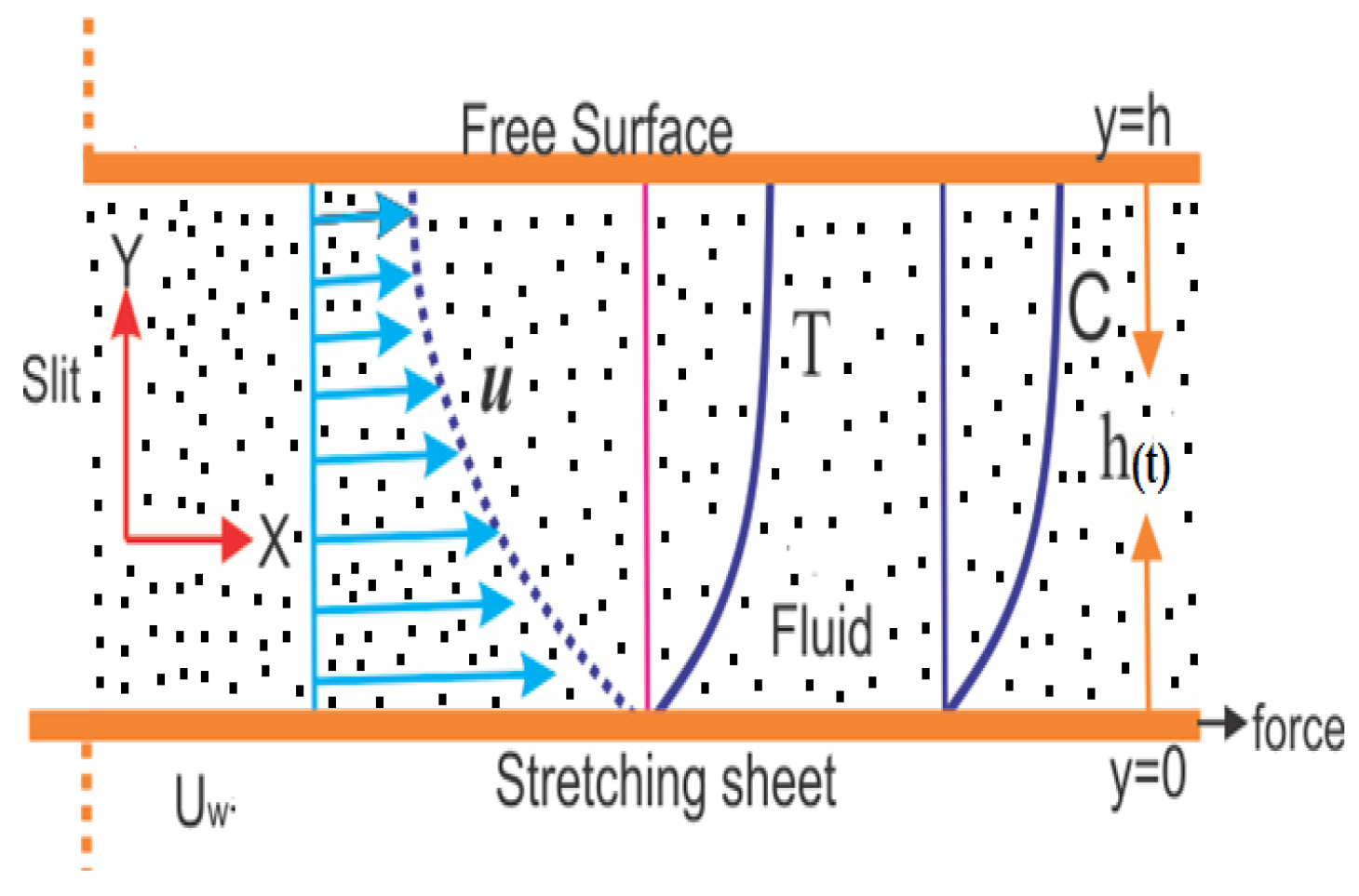
2. Mathematical Formulation of Model
3. Materials and Methods
Solution of Problem
4. Representation of Achieved Results in the Form of Figures and Tables
5. Results and Discussion
6. Conclusions
- (1)
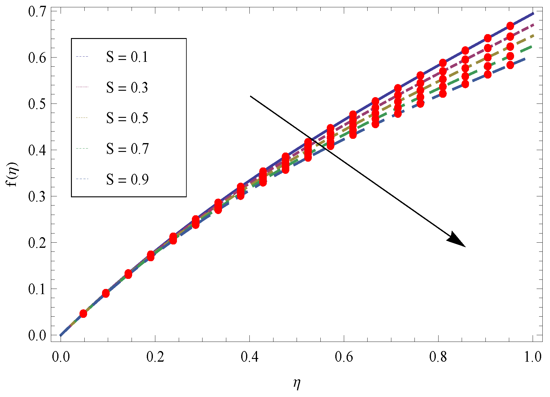
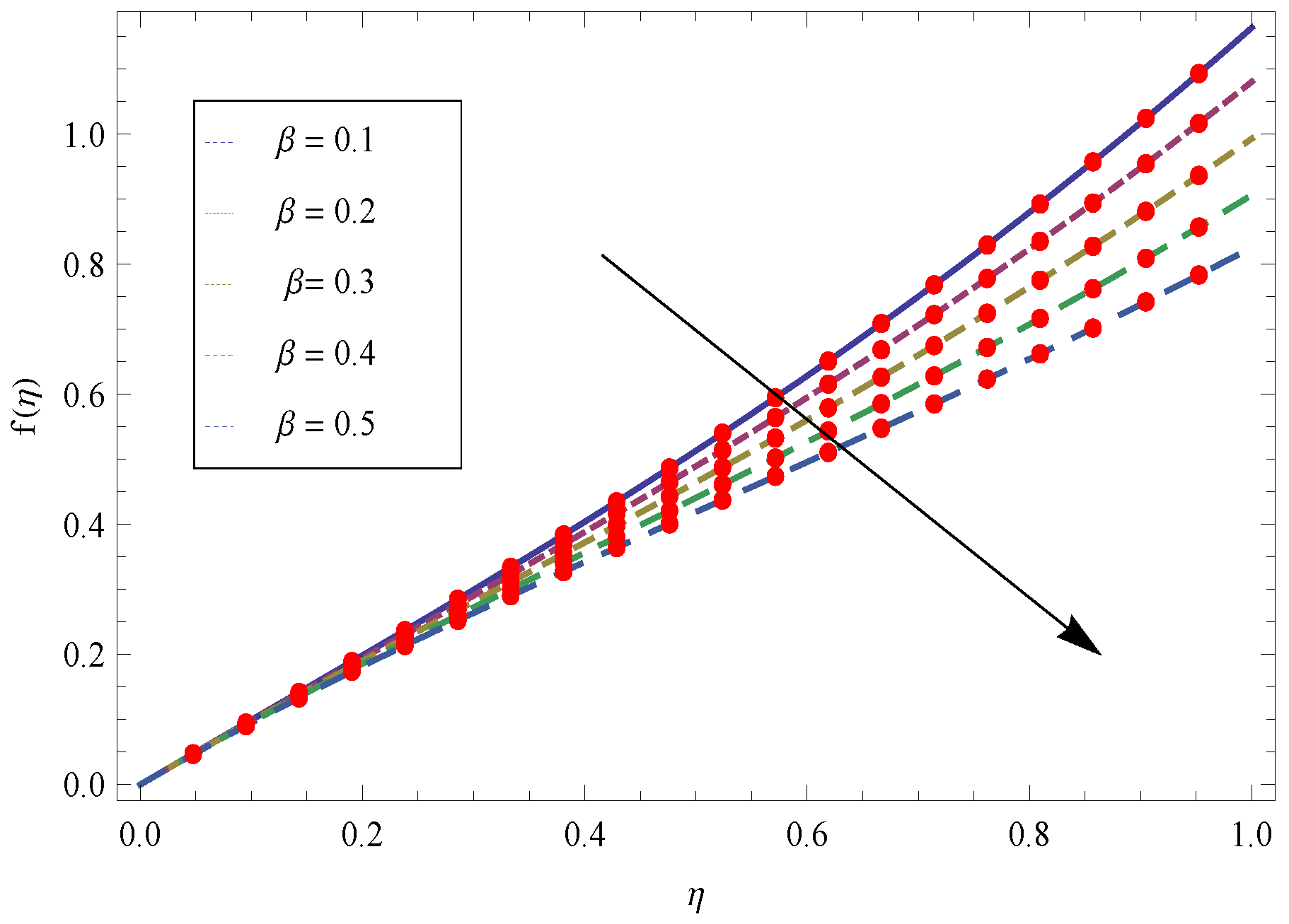
- Increasing thickness parameter produce the friction force and as a result velocity of the fluid film falls down.
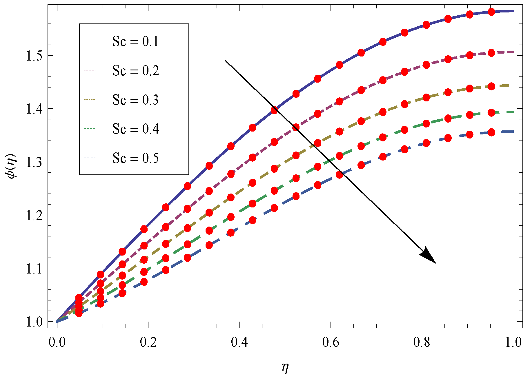
- (2)
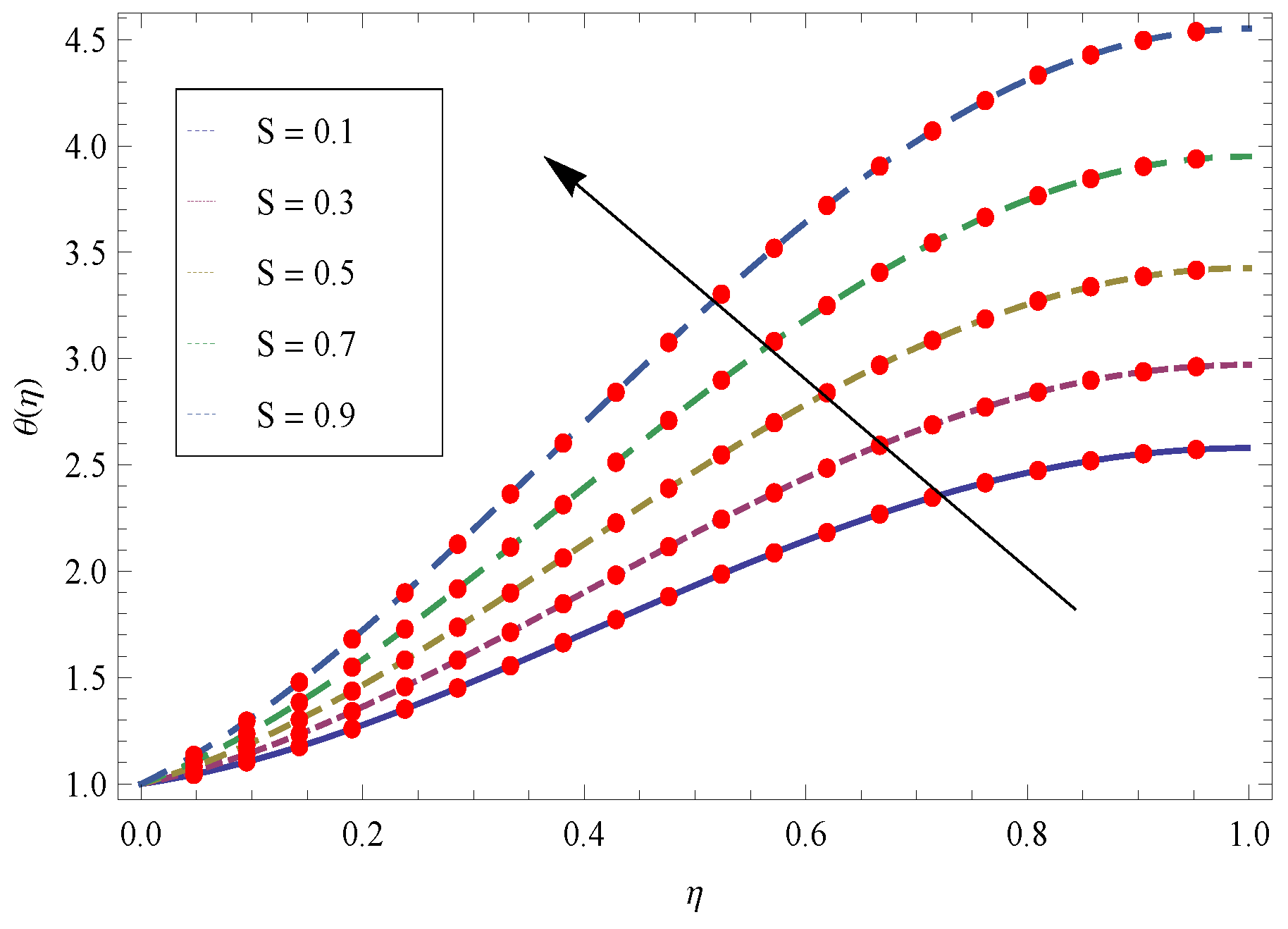
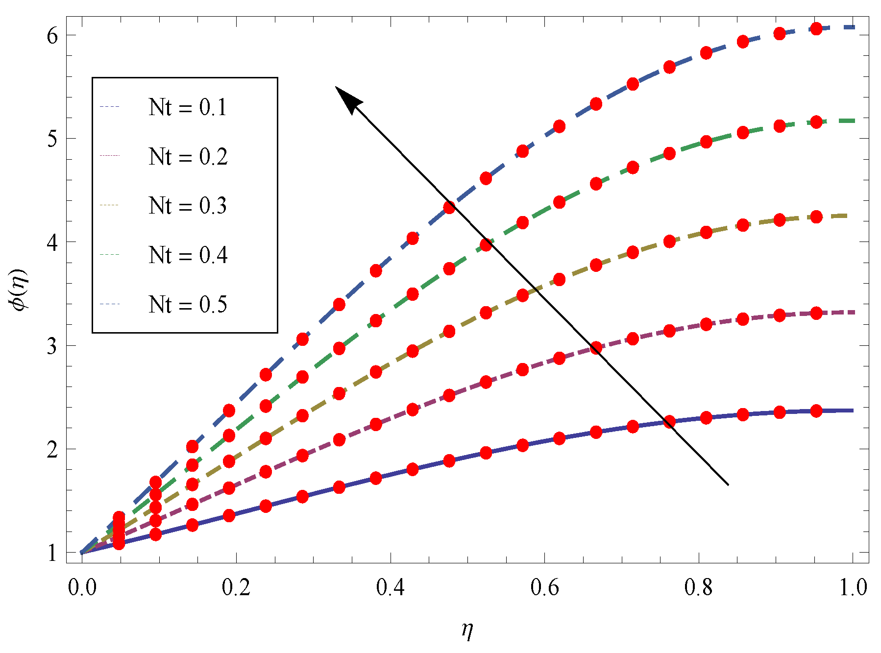
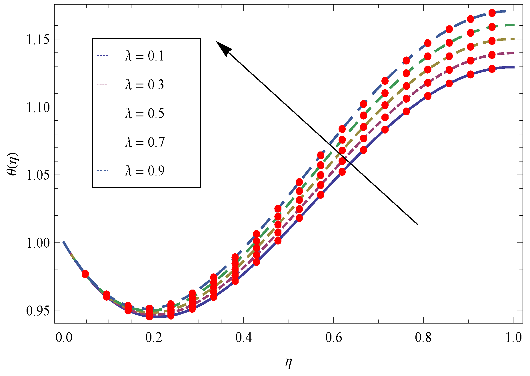
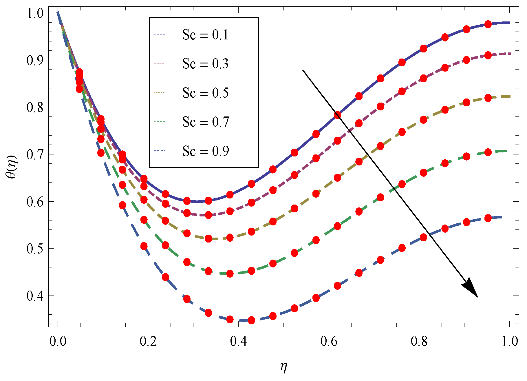
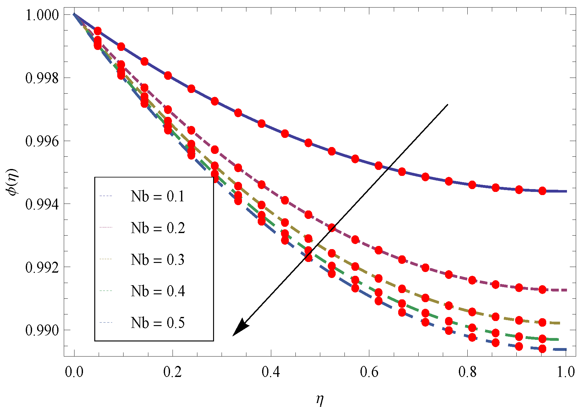
- The larger values of transport more fluid in the boundary layer region and cooling effect is produced which absorbed the heat transfer from the sheet and as a result the temperature reduces.
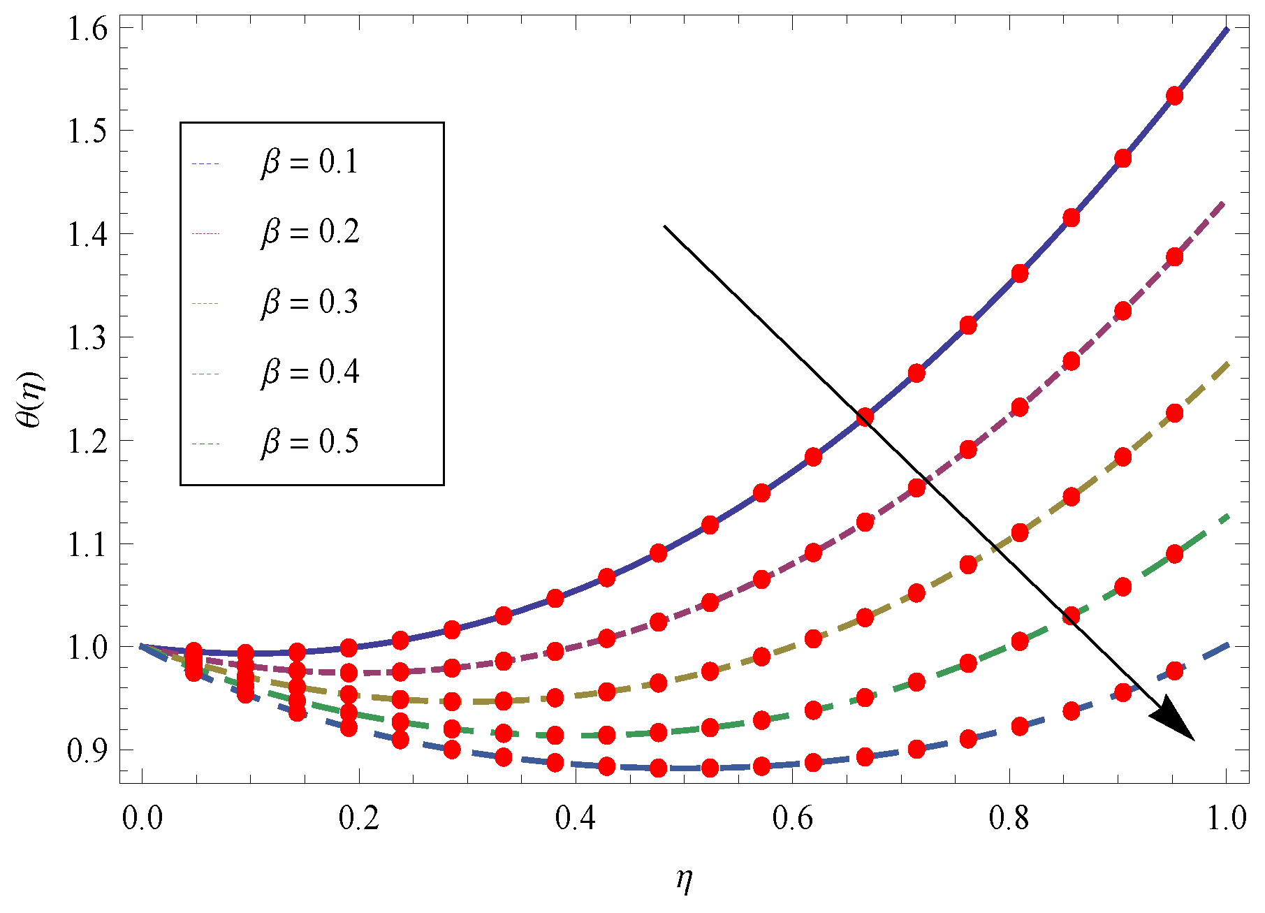
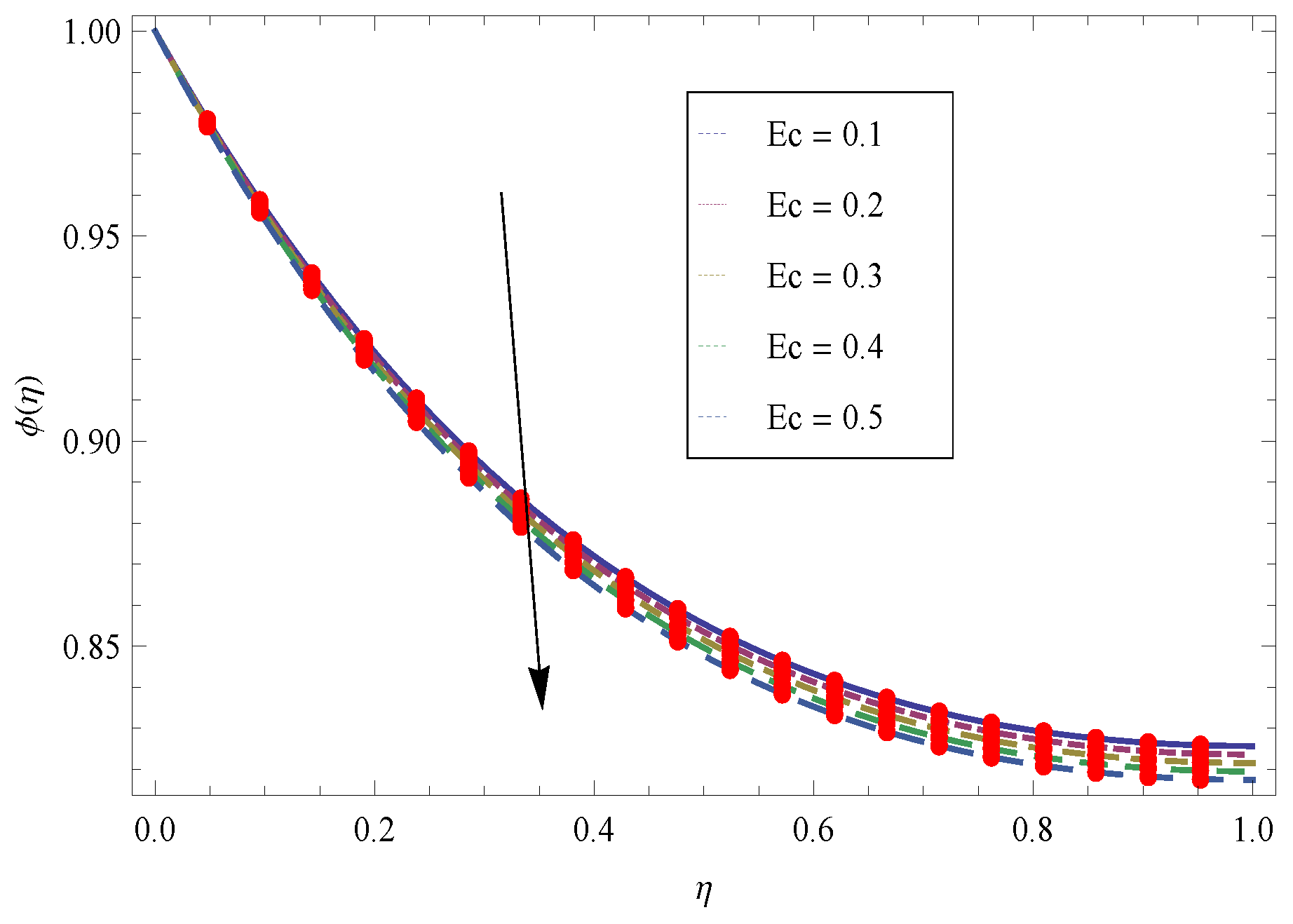
- (3)
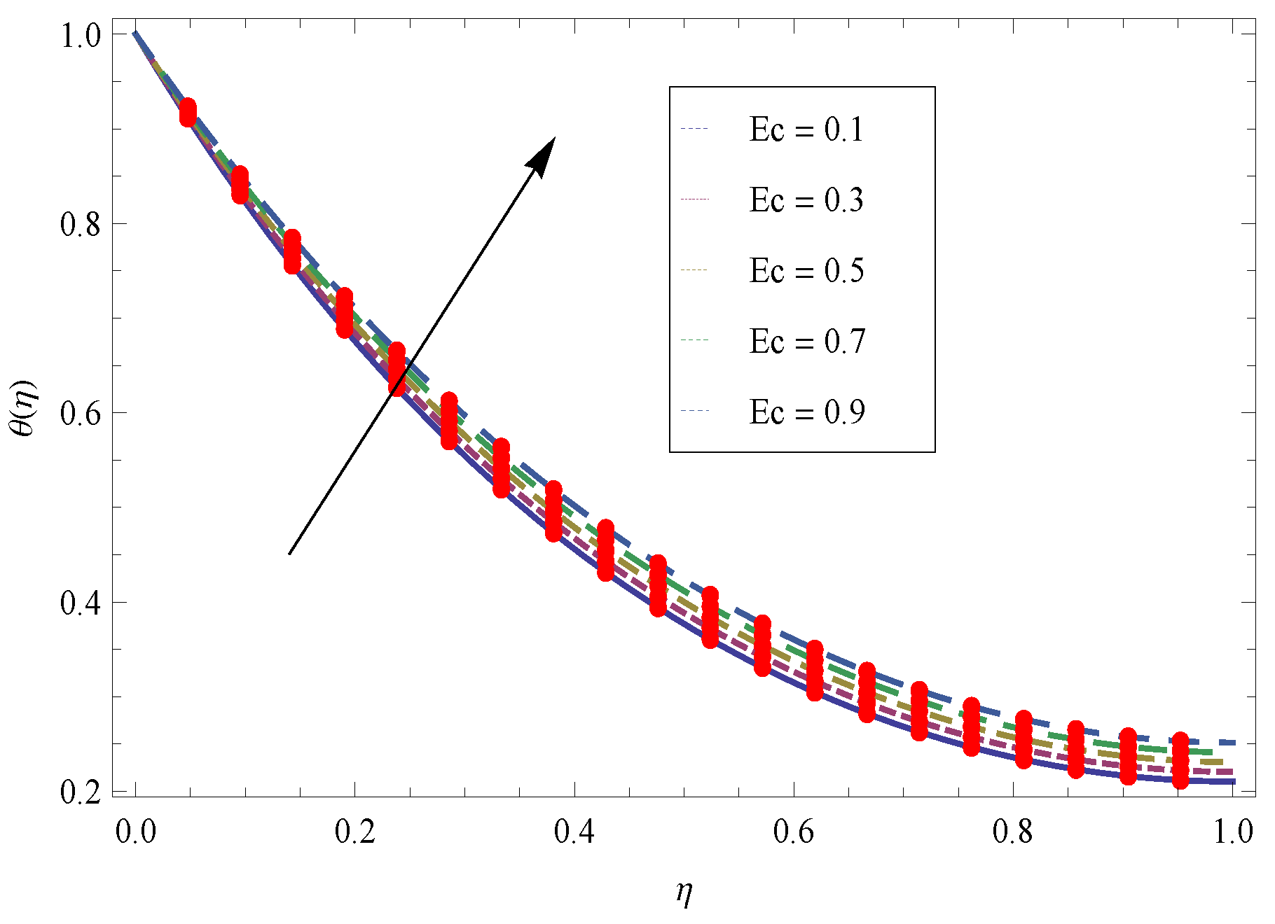
- The Eckert number is allied with the viscous dissipation term and lead to incrrease the quantity of heat being produced by the shear forces in the fluid. Therefore, larger values of raises the temperature field.
- (4)
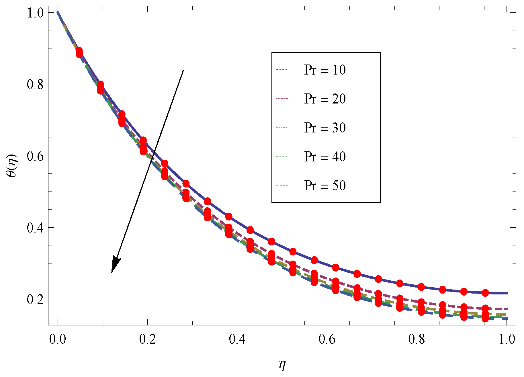
- The larger values of Prandtl number reduces the thermal boundary layer due to which the temperature field reduces.
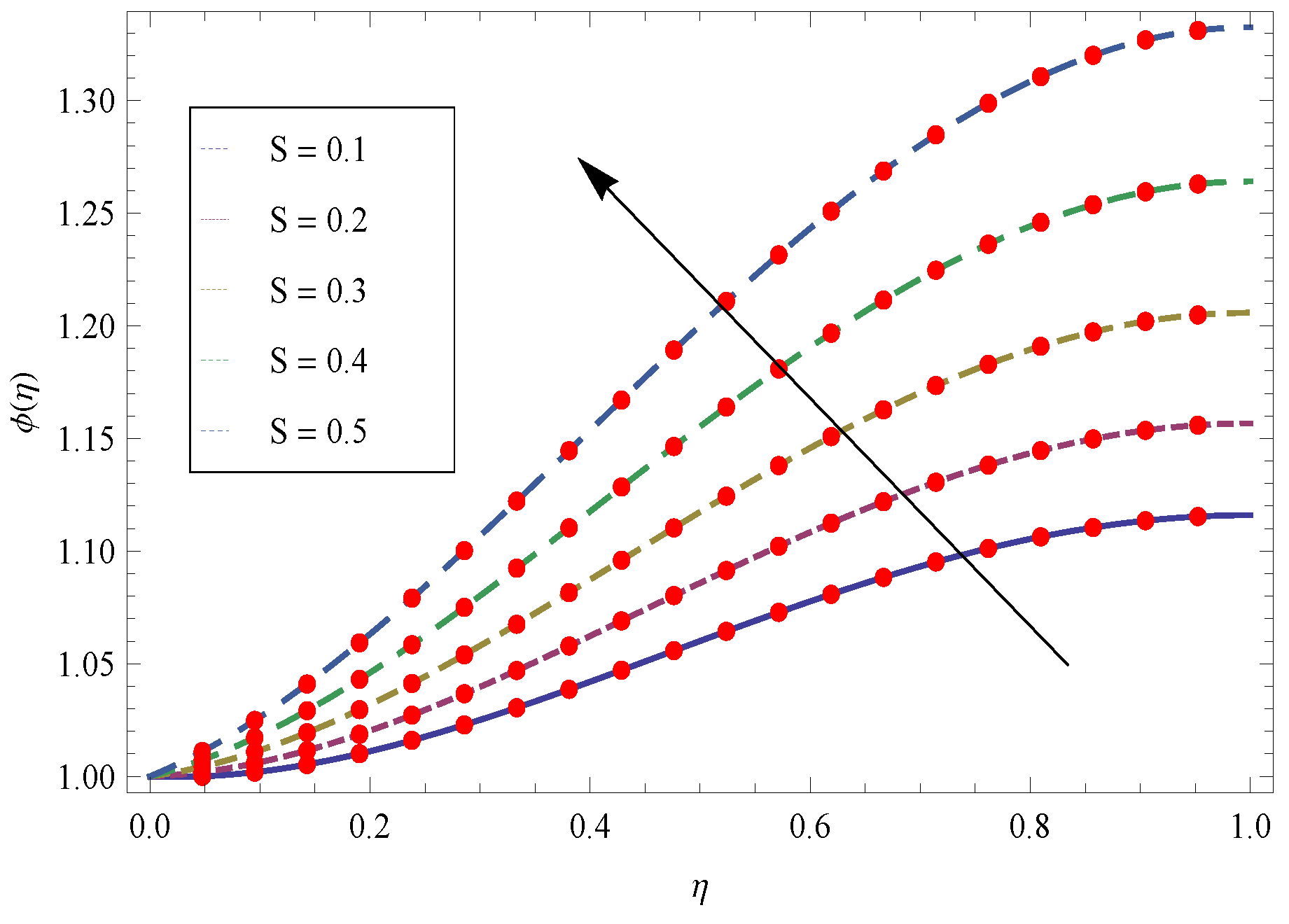
- (5)
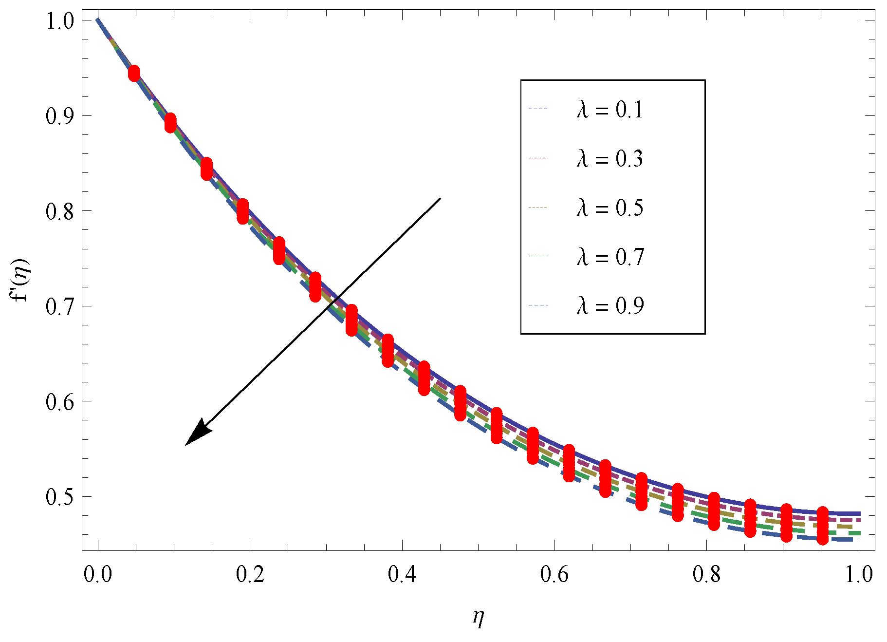
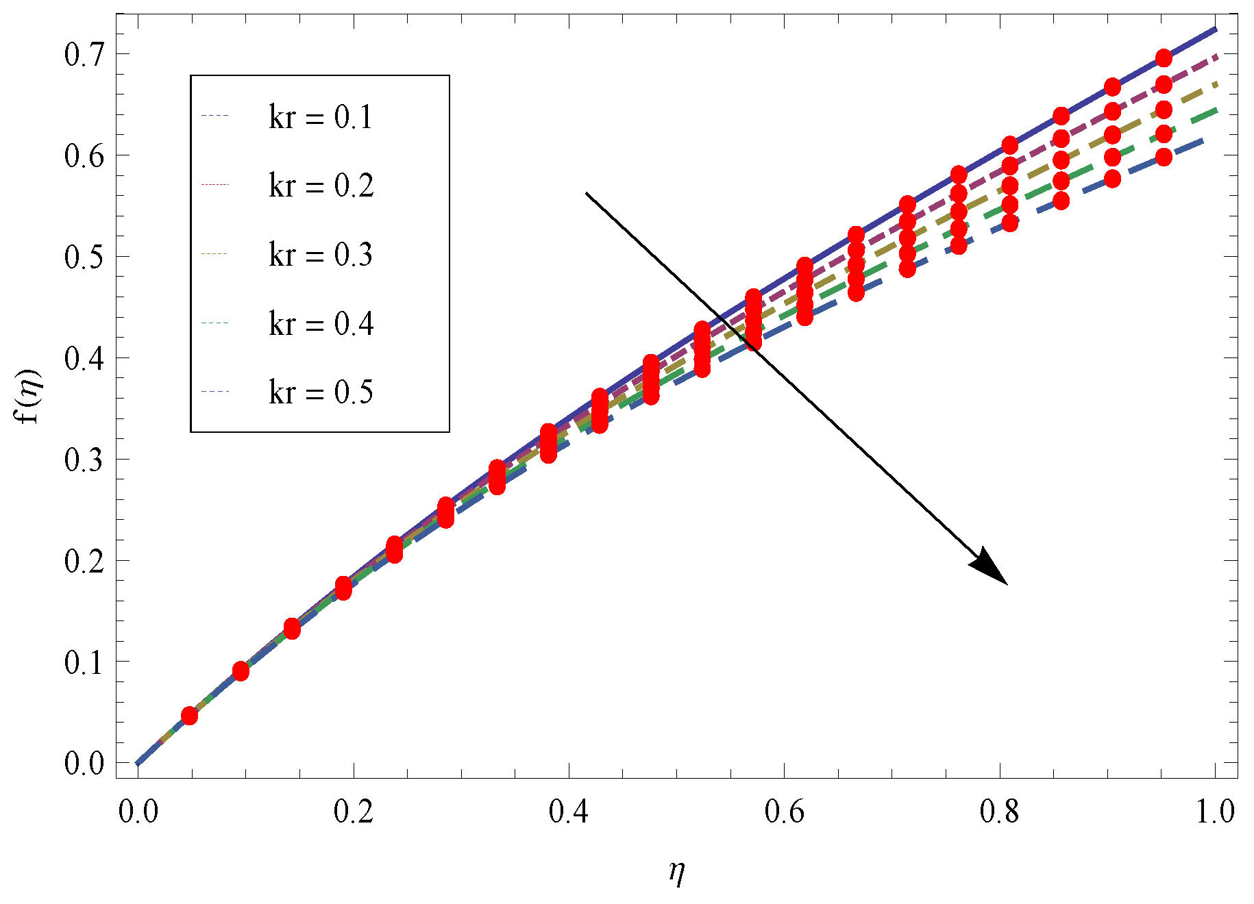
- Higher values of Porosity parameter generate larger open space and create hurdle to flow and as a result the flow field reduces.
Author Contributions
Conflicts of Interest
References
- Williamson, R.W. The dyanamics of lava flows. Annu. Rev. Fluid Mech. 2000, 32, 477–518. [Google Scholar]
- Dapra, I.; Scarpi, G. Perturbation solution for pulsatile flow of a non newtonian Williamson fluids in rock fracture. Int. J. Rock Mech. Min. Sci. 2006, 44, 1–8. [Google Scholar] [CrossRef]
- Wang, C.Y. Liquid film on an unsteady stretching surface. Q. Appl. Math. 1990, 48, 601–610. [Google Scholar] [CrossRef]
- Cramer, K.; Pai, S. Magneto Fluid Dynamics for Engineers and Applied Physicists; McGraw-Hill: New York, NY, USA, 1973. [Google Scholar]
- Selim, A.; Hossain, M.A.; Rees, D.A.S. The effect of surface mass transfer mixed convection flow past a heated vertical flat permeable plate with thermophoresis. Int. J. Therm. Sci 2003, 42, 973–982. [Google Scholar] [CrossRef]
- Das, K. Impact of thermal radiation on MHD slip flow over a flat plate with variable fluid properties. Heat Mass. Transf. 2012, 48, 767–778. [Google Scholar] [CrossRef]
- Siddeshwar, P.G.; Mahabaleshwar, U.S. Effects of radiation and heat transfer on MHD flow of viscoelastic liquid and heat transfer over a stretching sheet. Int. J. Nonlinear Mech. 2005, 40, 807–820. [Google Scholar] [CrossRef]
- Nadeem, S.; Hussain, S.T. Flow and heat transfer analysis of Williamson nanofluid. Appl. Nanosci. 2014, 4, 1005–1012. [Google Scholar] [CrossRef]
- Hassanein, I.A.; Essawy, A.; Morsy, N.M. Variable viscosity and thermal conductivity effects on heat transfer by natural convection from a cone and a wedge in porous media. Arch. Mech. 2004, 55, 345–356. [Google Scholar]
- Aziz, R.C.; Hashim, I.; Alomari, A.K. Thin film flow and heat transfer on an unsteady stretching sheet with internal heating. Meccanica 2011, 46, 349–357. [Google Scholar] [CrossRef]
- Qasim, M.; Khan, Z.H.; Lopez, R.J.; Khan, W.A. Heat and mass transfer in nanofluid over an unsteady stretching sheet using Buongiorno’s model. Eur. Phys. J. Plus 2016, 131, 1–16. [Google Scholar] [CrossRef]
- Mahesh, K.; Gireesha, B.J.; Rama, S.R.G. Heat and Mass Transfer in Nanofuid over an unsteady stretching surface. J. Nanofluids 2015, 4, 1–8. [Google Scholar]
- Ellahi, R.; Hassan, M.; Zeeshan, A. Aggregation effects on water base Al2O3-Nanofluid over permeable wedge in mixed convection. Asia-Pac. J. Chem. Eng. 2016, 11, 179–186. [Google Scholar] [CrossRef]
- Akbar, N.S.; Raza, M.; Ellahi, R. CNT suspended CuO + H2O nano fluid and energy analysis for the peristaltic flow in a permeable channel. Eng. J. 2015, 54, 623–633. [Google Scholar] [CrossRef]
- Akbar, N.S.; Raza, M.; Ellahi, R. Copper oxide nanoparticles analysis with water as base fluid for peristaltic flow in permeable tube with heat transfer. Comput. Methods Progr. Biomed. 2016, 130, 22–30. [Google Scholar] [CrossRef]
- Shehzad, N.; Zeeshan, A.; Ellahi, R.; Vafai, K. Convective heat transfer of nanofluid in a wavy channel: Buongiorno’s mathematical model. J. Mol. Liq. 2016, 222, 446–455. [Google Scholar] [CrossRef]
- Zeeshan, A.; Hassan, M.; Ellahi, R.; Nawaz, M. Shape effect of nanosize particles in unsteady mixed convection flow of nanofluid over disk with entropy generation. J. Process Mech. Eng. 2016. [Google Scholar] [CrossRef]
- Khan, W.; Gul, T.; Idrees, M.; Islam, I.; Khan, I.; Dennis, L.C.C. Thin Film Williamson Nanofluid Flow with Varying Viscosity and Thermal Conductivity on a Time-Dependent Stretching Sheet. Appl. Sci. 2016, 6, 334. [Google Scholar] [CrossRef]
- Gamal, M.; Rahman, A. Effect of Magnetohydrodynamic on Thin Films of Unsteady Micropolar Fluid through a Porous Medium. J. Mod. Phys. 2011, 2, 1290–1304. [Google Scholar]
- Jaina, S.; Choudhary, R. Effects of MHD on Boundary Layer Flow in Porous Medium due to Exponentially Shrinking Sheet with Slip. Procedia Eng. 2015, 127, 1203–1210. [Google Scholar] [CrossRef]
- Liao, S. Beyond Perturbation: Introduction to the Homotopy Analysis Method; Chapman and Hall/CRC: Boca Raton, FL, USA, 2003. [Google Scholar]
- Liao, S.J. An optimal homotopy-analysis approach for strongly nonlinear differential equations. Commun. Nonlinear Sci. Numer. Simul. 2010, 15, 2003–2016. [Google Scholar] [CrossRef]
- Liao, S. On the homotopy analysis method for nonlinear problems. Appl. Math. Comput. 2004, 147, 499–513. [Google Scholar] [CrossRef]
- Abbasbandy, S.; Shirzadi, A. A new application of the homotopy analysis method: Solving the Sturm—Liouville problems. Commun. Nonlinear Sci. Numer. Simul. 2011, 16, 112–126. [Google Scholar] [CrossRef]
- Abbasbandy, S. Homotopy analysis method for heat radiation equations. Int. Commun. Heat Mass Transf. 2007, 34, 380–388. [Google Scholar] [CrossRef]
- Abbasbandy, S. The application of homotopy analysis method to solve a generalized Hirota-Satsuma coupled KdV equation. Phys. Lett. A 2007, 361, 478–483. [Google Scholar] [CrossRef]
- Khan, N.S.; Taza Gul, T.; Islam, S.; Khan, W. Thermophoresis and thermal radiation with heat and mass transfer in a magnetohydrodynamic thin film second grade fluid of variable properties past a stretching sheet. Eur. Phys. J. Plus 2017, 132. [Google Scholar] [CrossRef]
- Khan, W.; Gul, T.; Idrees, M.; Khan, I. Dufour and Soret Effect with Thermal Radiation on the Nano Film Flow of Williamson Fluid Past Over an Unsteady Stretching Sheet. J. Nanofluids 2017, 6, 243–253. [Google Scholar]
- Narayana, M.; Sibanda, P. Hydromagnetic nanofluid flow due to a stretching or shrinking sheet with viscous dissipation and chemical reaction effects. Int. J. Heat Mass. Transf. 2012, 55, 7587–7595. [Google Scholar]
- Xu, H.; Pop, I.; You, X.C. Flow and heat transfer in a nano-liquid film over an unsteady stretch surface. Int. J. Heat Mass. Transf. 2013, 60, 646–652. [Google Scholar] [CrossRef]
- Nadeem, S.; Haq, R.U.; Lee, C. MHD flow of a Casson fluid over an exponentially shrinking sheet. Sci. Iran. 2012, 19, 1550–1553. [Google Scholar] [CrossRef]
- Nadeem, S.; Haq, R.U.; Akbar, N.S.; Khan, Z.H. MHD three-dimensional Casson fluid flow past a porous linearly stretching sheet. Alex. Eng. J. 2013, 52, 577–582. [Google Scholar] [CrossRef]
- Rehman, S.U.; Haq, R.U.; Lee, C.; Nadeem, S. Numerical study of non-Newtonian fluid flow over an exponentially stretching surface: an optimal HAM validation. Braz. Soc. Mech. Sci. Eng. 2016, 7. [Google Scholar] [CrossRef]
- Haq, R.U.; Shahzad, F.; Al-Mdallal, Q.M. MHD Pulsatile Flow of Engine oil based Carbon Nanotubes between Two Concentric Cylinders. Results Phys. 2016, 7, 57–68. [Google Scholar] [CrossRef]
- Besthapu, P.; Haq, R.U.; Bandari, S.; Al-Mdallal, Q.M. Mixed convection flow of thermally stratified MHD nanofluid over an exponentially stretching surface with viscous dissipation effect. J. Taiwan Inst. Chem. Eng. 2017, 71, 307–314. [Google Scholar] [CrossRef]


| Alphabet | Defined as | Alphabet | Defined as |
| x | horizontal coordinate | Reference temperature | |
| y | vertical coordinate | initial temperature of the fluid (K) | |
| u | horizontal velocity component (m/s) | T | temperature (K) |
| v | vertical velocity component (m/s) | Velocity of the stretching sheet | |
| S | Unsteadiness parameter | final temperature of the fluid (K) | |
| Temperature at the sheet | T | temperature (K) | |
| K | thermal diffusivity (m) | t | time (s) |
| S | Unsteadiness parameter | f | Dimensionless Velocity |
| b | stretching parameter(constant) | k | permeability coefficient of the porosity |
| nondimensional variable for velocity | Nanoparticle volume fraction at sheet | ||
| Prandtl number | Eckert number | ||
| nondimensional porosity parameter | Sc | Schmidt number | |
| Brownian motion parameter | Brownian diffusion coefficient | ||
| specific heat at constant pressure (kJ kg K) | Thermophoresis parameter | ||
| Greek symbols | Defined as | Greek Symbols | Defined as |
| Dimensionless nanoparticle volume fraction | Similarity variable | ||
| kinematic viscosity of the fluid | Density of base fluid | ||
| density (kg m) | Heat capacity of the nanoparticle material | ||
| Time constant | Thermal diffusivity of the base fluid | ||
| Nanoparticle mass density | Heat capacity of the base fluid | ||
| Kinematic viscosity of the base fluid | Williamson fluid constant | ||
| non-dimensional film thickness | Dimensionless temperature | ||
| non-dimensional stream function | differentiation w. r. t. |
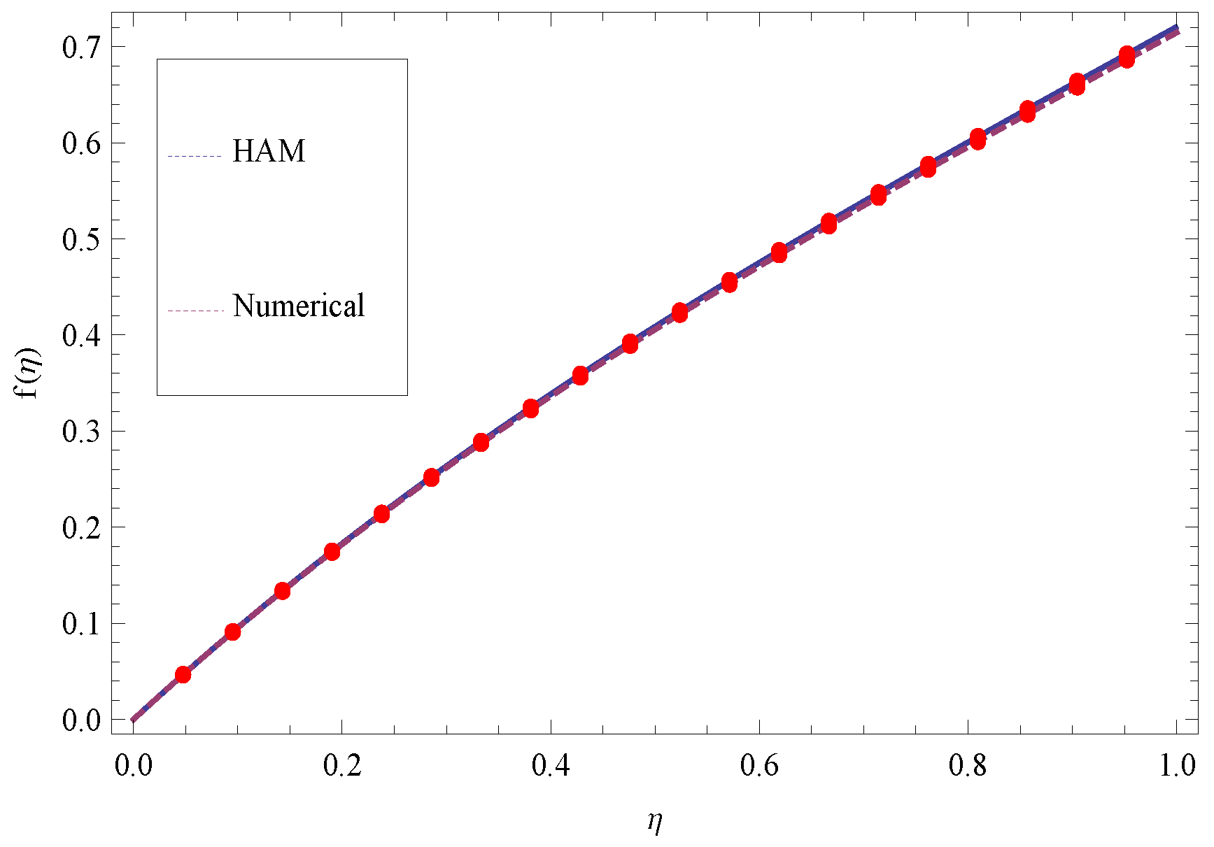
| Numerical Solution for | HAM Solution for | Absolute Error | |
|---|---|---|---|
| 0 | 0 | 0 | 0 |
| 0.1 | 0.0952761 | 0.0955184 | |
| 0.2 | 0.182152 | 0.182958 | |
| 0.3 | 0.262045 | 0.263561 | |
| 0.4 | 0.336198 | 0.338462 | |
| 0.5 | 0.405709 | 0.408698 | |
| 0.6 | 0.471556 | 0.47522 | |
| 0.7 | 0.534618 | 0.5389 | |
| 0.8 | 0.595686 | 0.600535 | |
| 0.9 | 0.655482 | 0.660862 | |
| 1 | 0.714666 | 0.720558 |
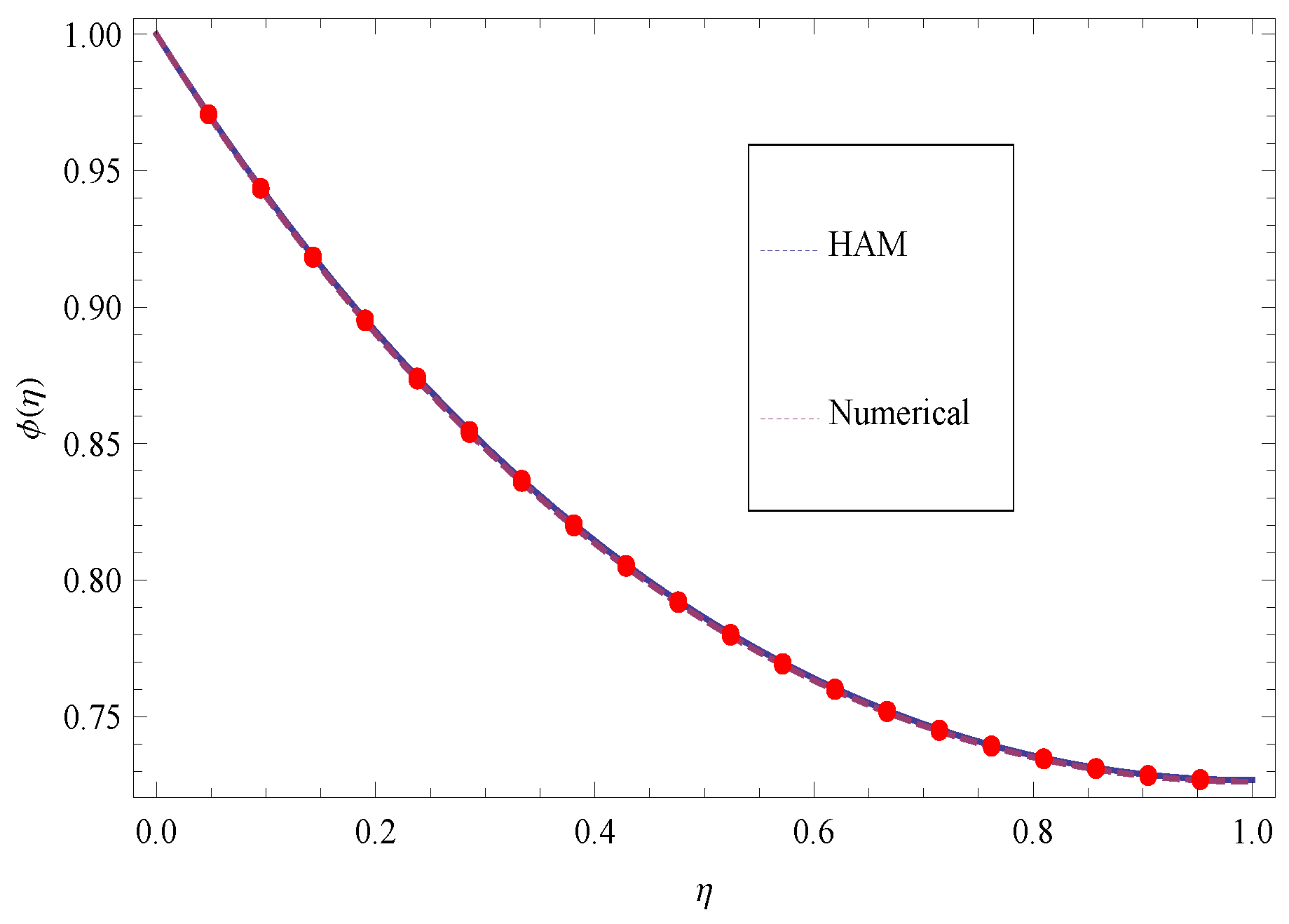
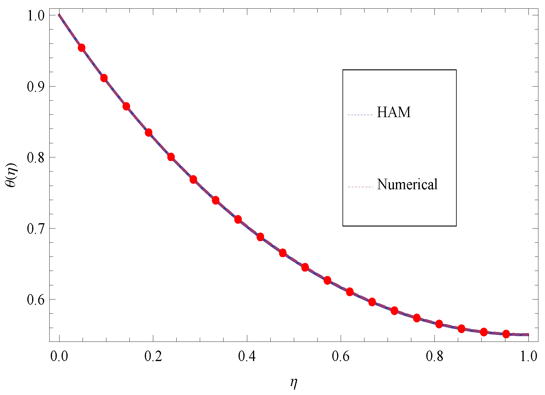
| Numerical Solution for | HAM Solution for | Absolute Error | |
|---|---|---|---|
| 0 | 1 | 1 | |
| 0.1 | 0.907342 | 0.90737 | |
| 0.2 | 0.82775 | 0.827596 | |
| 0.3 | 0.759861 | 0.759482 | |
| 0.4 | 0.702621 | 0.702067 | |
| 0.5 | 0.655233 | 0.654586 | |
| 0.6 | 0.617098 | 0.616438 | |
| 0.7 | 0.587786 | 0.587169 | |
| 0.8 | 0.567002 | 0.566451 | |
| 0.9 | 0.554573 | 0.554078 | |
| 1 | 0.550428 | 0.549956 |
| Numerical Solution for | HAM Solution for | Absolute Error | |
|---|---|---|---|
| 0 | 1 | 1 | |
| 0.1 | 0.940581 | 0.941167 | |
| 0.2 | 0.890316 | 0.8912 | |
| 0.3 | 0.848224 | 0.849209 | |
| 0.4 | 0.813465 | 0.81443 | |
| 0.5 | 0.785325 | 0.786207 | |
| 0.6 | 0.763201 | 0.76398 | |
| 0.7 | 0.74659 | 0.747277 | |
| 0.8 | 0.735082 | 0.735705 | |
| 0.9 | 0.728352 | 0.728942 | |
| 1 | 0.726151 | 0.726734 |
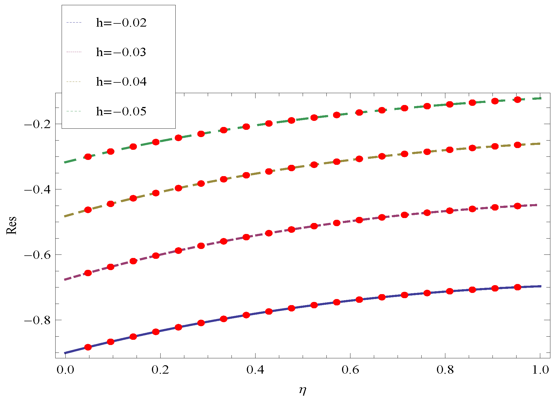
| Residuals for | Residuals for | Residuals for | |
|---|---|---|---|
| 0 | |||
| 0.1 | |||
| 0.2 | |||
| 0.3 | |||
| 0.4 | |||
| 0.5 | |||
| 0.6 | |||
| 0.7 | |||
| 0.8 | |||
| 0.9 | |||
| 1 |
© 2017 by the authors. Licensee MDPI, Basel, Switzerland. This article is an open access article distributed under the terms and conditions of the Creative Commons Attribution (CC BY) license (http://creativecommons.org/licenses/by/4.0/).
Share and Cite
Ali, L.; Islam, S.; Gul, T.; Khan, I.; Dennis, L.C.C.; Khan, W.; Khan, A. The Brownian and Thermophoretic Analysis of the Non-Newtonian Williamson Fluid Flow of Thin Film in a Porous Space over an Unstable Stretching Surface. Appl. Sci. 2017, 7, 404. https://doi.org/10.3390/app7040404
Ali L, Islam S, Gul T, Khan I, Dennis LCC, Khan W, Khan A. The Brownian and Thermophoretic Analysis of the Non-Newtonian Williamson Fluid Flow of Thin Film in a Porous Space over an Unstable Stretching Surface. Applied Sciences. 2017; 7(4):404. https://doi.org/10.3390/app7040404
Chicago/Turabian StyleAli, Liaqat, Saeed Islam, Taza Gul, Ilyas Khan, L. C. C. Dennis, Waris Khan, and Aurangzeb Khan. 2017. "The Brownian and Thermophoretic Analysis of the Non-Newtonian Williamson Fluid Flow of Thin Film in a Porous Space over an Unstable Stretching Surface" Applied Sciences 7, no. 4: 404. https://doi.org/10.3390/app7040404