An Automatic Measurement Method for Absolute Depth of Objects in Two Monocular Images Based on SIFT Feature

Abstract

Recovering depth information of objects from two-dimensional images is one of the very important and basic problems in the field of computer vision. In view of the shortcomings of existing methods of depth estimation, a novel approach based on SIFT (the Scale Invariant Feature Transform) is presented in this paper. The approach can estimate the depths of objects in two images which are captured by an un-calibrated ordinary monocular camera. In this approach, above all, the first image is captured. All of the camera parameters remain unchanged, and the second image is acquired after moving the camera a distance d along the optical axis. Then image segmentation and SIFT feature extraction are implemented on the two images separately, and objects in the images are matched. Lastly, an object’s depth can be computed by the lengths of a pair of straight line segments. In order to ensure that the most appropriate pair of straight line segments are chosen, and also reduce computation, convex hull theory and knowledge of triangle similarity are employed. The experimental results show our approach is effective and practical.

1. Introduction

Acquiring depth information from two-dimensional images is one of the fundamental problems in machine vision, and it can be applied to many fields such as the restoration of 3D scenes, planning of robot walking route, etc. In particular, the depths of interesting objects in images are very useful; for instance, the distances from obstacles in the road, frontal vehicles, and traffic lights must be known when an unmanned vehicle is running on the road. The depth information can also be used for pattern recognition [1,2].

At present, the methods of obtaining the depth information of objects in 2D images fall mainly into two major categories: stereo vision based on binocular (or multi-nocular) [3,4,5], and stereo vision based on monocular. At least two camera devices must be provided in the first class of method. Each camera’s intrinsic parameters and the parameters of the spatial relationship between any two cameras are also provided. This means that camera calibration is needed in the first class of method. Bumblebee is a kind of product for stereo vision based on binocular, and a light-field camera can also get the depth information from its micro-lens array [6,7,8,9,10]. But both of them are expensive.

The second class of method includes Depth From Focus (DFF) and Depth From Defocus (DFD). In the DFF method [11,12], a lot of images of the same scene with different camera optical parameters are taken. Then, a full focus image is formed by using the pixels which are in focus in the images. Finally, the depth map can be obtained by analyzing every pixel in the full focus image and the camera parameters when the pixel is obtained. Only one camera is needed in this method, but its application is very limited, for a large number of images of the same scene must be taken.

The DFD was first proposed by Pentland [13] in 1987, and was improved by Subbarao [14] and Rajagopalan [15]. In 2008, defocus was modeled as an anisotropic thermal diffusion process by Favaro [16] et al., and this improvement has a better result. But two or more images which are taken in different cameras need to be supplied in the above improved method. Zhou and Sim [17] presented an original approach that depth map could be estimated from a single defocused image. In this method, firstly, the defocused image is re-blurred using a known Gaussian kernel. Then the depth information at the edge in image can be obtained by the ratio between the gradient of the defocused image and the re-blurred one. Finally, the depth at edge locations is propagated to the entire image by solving the optimization problem. None of the above approaches based on defocusing could tell the reason for blurred edges in an image, which can be caused by either blur texture ambiguity or focal plane ambiguity. And they could not get the absolute depth information unless the camera was calibrated.

The coded aperture method proposed by Zhou [18] et al. could estimate a better depth map, but the shape of camera aperture must be modified. Kouskouridas [19] et al. used SIFT (the Scale Invariant Feature Transform) to acquire the absolute depth of the objects in image. In this method, a database must first be built. The database contains 5 or more images which are taken from different object distances or angles of view to every object measured. The object distances are acquired by a laser device and stored in the database. The data in the database will be used to train the algorithm. It is not able to estimate the depth of an object if the object is not in the database. This means it can only compute the absolute depth of an object that has been stored in the database. This approach has a complex operation step and a limited application scope. Fang [20] employed a structure forest framework to extract the depth information from a single color image. The method can achieve quasi real-time performance, but the accuracy needs to be improved, especially for indoor scenes.

In this paper, we propose a novel approach to compute the absolute depth of target objects (it is given beforehand which objects are target objects). It only needs a monocular camera and no calibrating. Firstly, the image A is captured, and then the image B is captured after moving the camera a distance d along the optical axis. The camera’s intrinsic parameters are kept constant during the whole process. Secondly, we get the objects by segmenting the two images. Simultaneously, the SIFT points are detected in the two images. The image of the same object in the two images should be matched after completing the SIFT point matching. Finally, the absolute depth of an object can be computed by using the corresponding lengths of two straight line segments in the two images. The first straight line segment is composed of two SIFT feature points in image A, and the second one is composed of two corresponding matching SIFT feature points in image B.

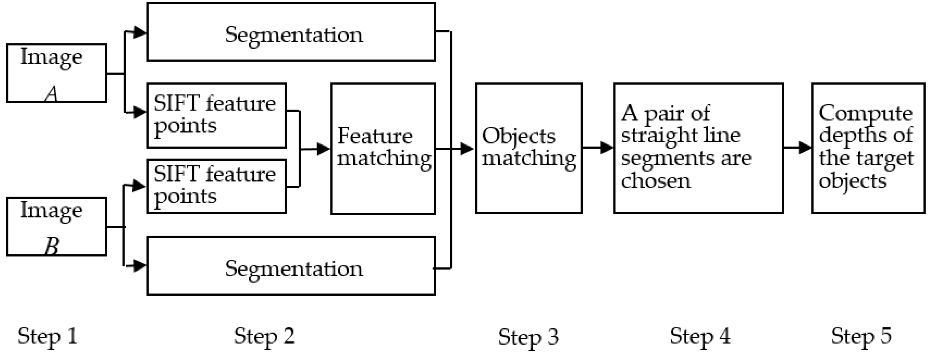
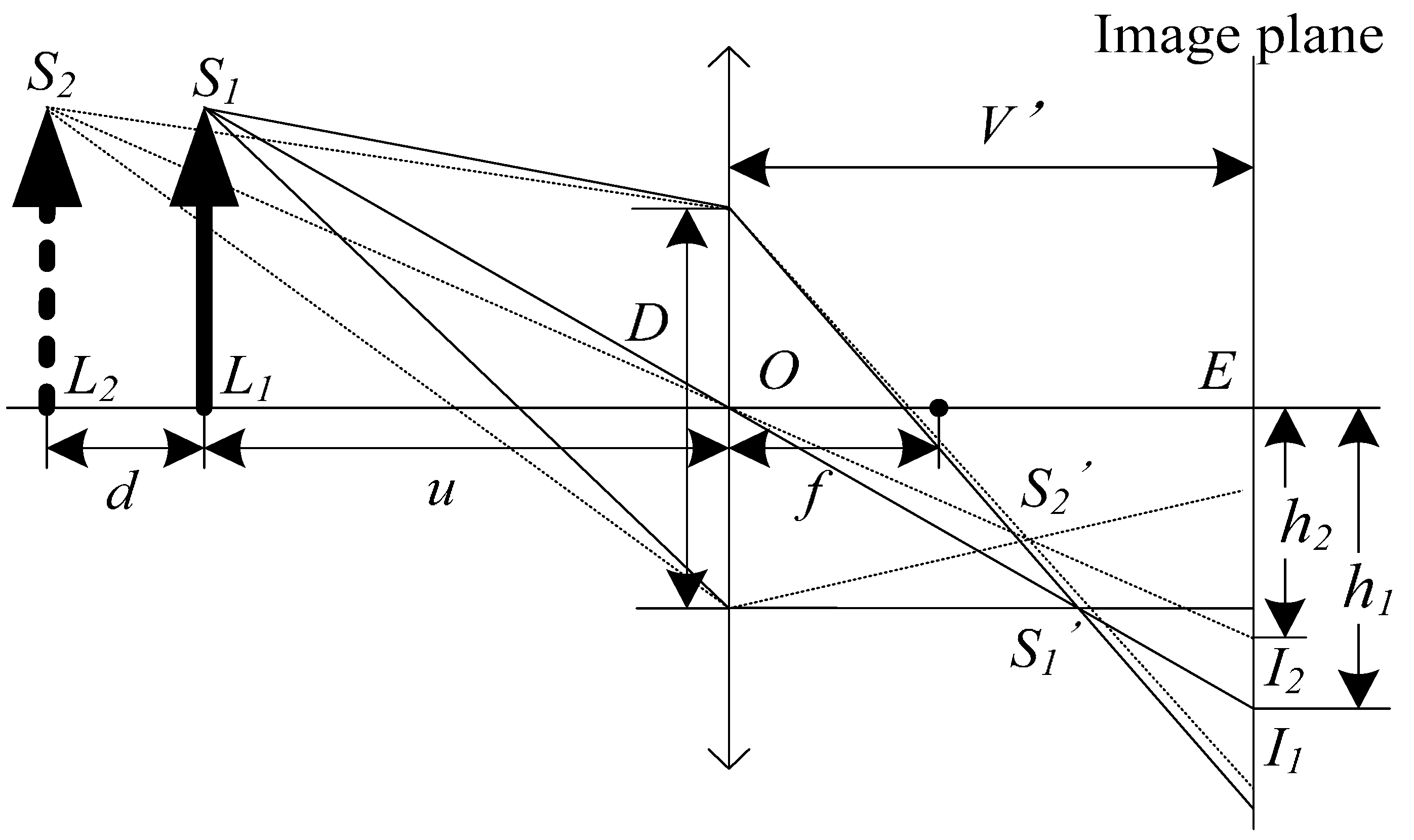
2. The Basic Principles and Algorithm Steps

The basic principles of imaging can be modeled as

$$\frac{1}{f}=\frac{1}{u}+\frac{1}{v}$$

(1)

where f is the focal length. u is object distance (namely depth), and v is the distance between the image plane and lens.

As show in Figure 1, we assume that the object distance is u and the high of image of object is h₁ in the first photograph. In the second one, they are u + d and h₂, respectively. Because the camera’s intrinsic properties are unchanged between the two photographs, the relation of h₁ and h₂ can be formulated as

$$h_2=k{h}_1$$

(2)

where k > 0 and k $\in$ R, and R is the set of real numbers.

According to the basic principles of imaging and the knowledge of triangles, the object distance u can be computed by the following formulation.

$$u=\frac{h_2}{h_1-h_2}d$$

(3)

Usually, h₁ and h₂ are the heights of the images of object. In fact, they can be the distance of two feature points on an object, too. Therefore, we can compute the depth u if we detect two pairs of corresponding feature points of the same object in two images.

Figure 2 shows the overview of our method of estimating the object depth. It mainly includes 5 steps as follows:

Step 1:

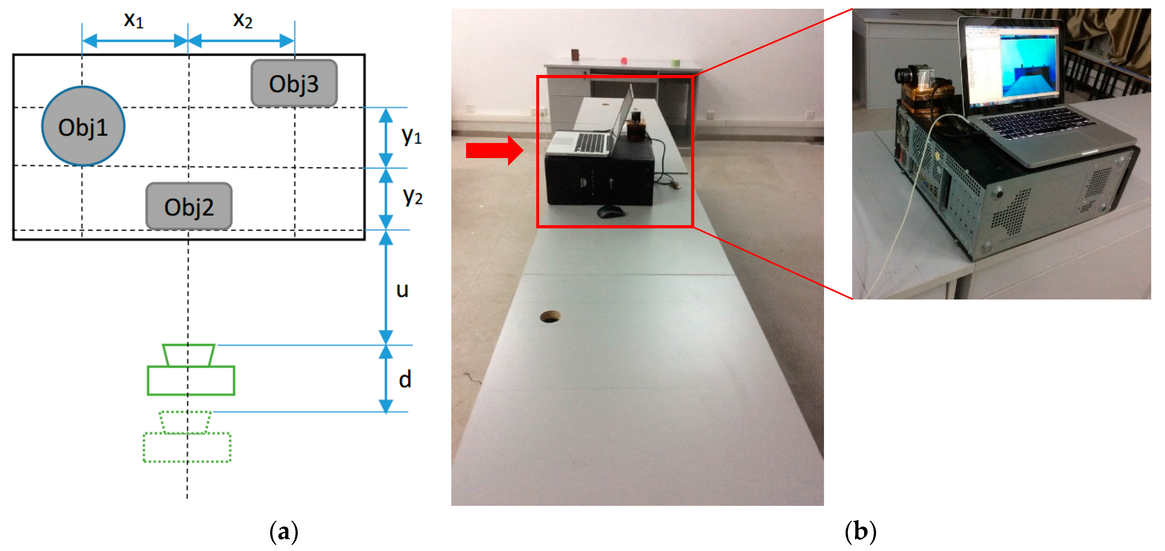
Holding the camera constant, we take the image A and B when the object distance is u and u + d, respectively.

Step 2:

Images of objects (namely sub-regions) are obtained by segmenting the image A and B, respectively. Meanwhile, we detect the SIFT feature points in the image A and B, then, match the points.

Step 3:

Using the results of segmentation and matching of feature points, we can match the images of objects.

Step 4:

A pair of straight line segments are chosen from the image A and B. During the process, the theory of the convex hull is used to decrease the computational complexity, and the knowledge of the similarity triangle is used to avoid the wrong straight line straight being chosen. The lengths of the pair of straight line segments will be used to compute the depth of the object.

Step 5:

The depth of the object can be computed by the length of the pair of straight line segments.

3. Matching the Images of Objects

Matching the images of objects cannot be done unless both the segmentation and detection of SIFT feature points has been completed. At present, there are a number of methods of segmentation. The LBF (Local Binary Fitting Energy) method [21,22] is employed in this paper, because it has a better segmentation result, especially for images with intensity inhomogeneity. The SIFT feature points are invariant to image scale and rotation, with robust matching across a substantial range of affine distortion, addition of noise, and change in illumination [23,24].

We assume that the image A is partitioned into m subregions by the LBF image segmentation approach. The m subregions are A₁, A₂, …, A_m, and X_i is the SIFT feature points set of the A_i subregion. where i = 1, 2, …, m. Similarly, the image B is segmented into n subregions: B₁, B₂, …, B_n, and Y_j is the SIFT feature points set of B_j. where j = 1, 2, …, n. Z_i is the matching feature points set of X_i. Therefore, Z_i ⊆ (Y₁∪Y₂∪…∪Y_n). The card(S) means the number of elements in the set S.

$$Y_k=\underset{Y_j}{\arg \max }(card(Z_i\cap Y_j))$$

(4)

$$\frac{card(Y_k)}{card(X_i)}>T_p$$

(5)

where T_p is a threshold. The object A_i is matched with B_k if both the Formulas (4) and (5) are satisfied, namely, the subregion A_i in image A and the subregion B_k in image B are the images of the same object.

4. Selecting the Straight Line Segments

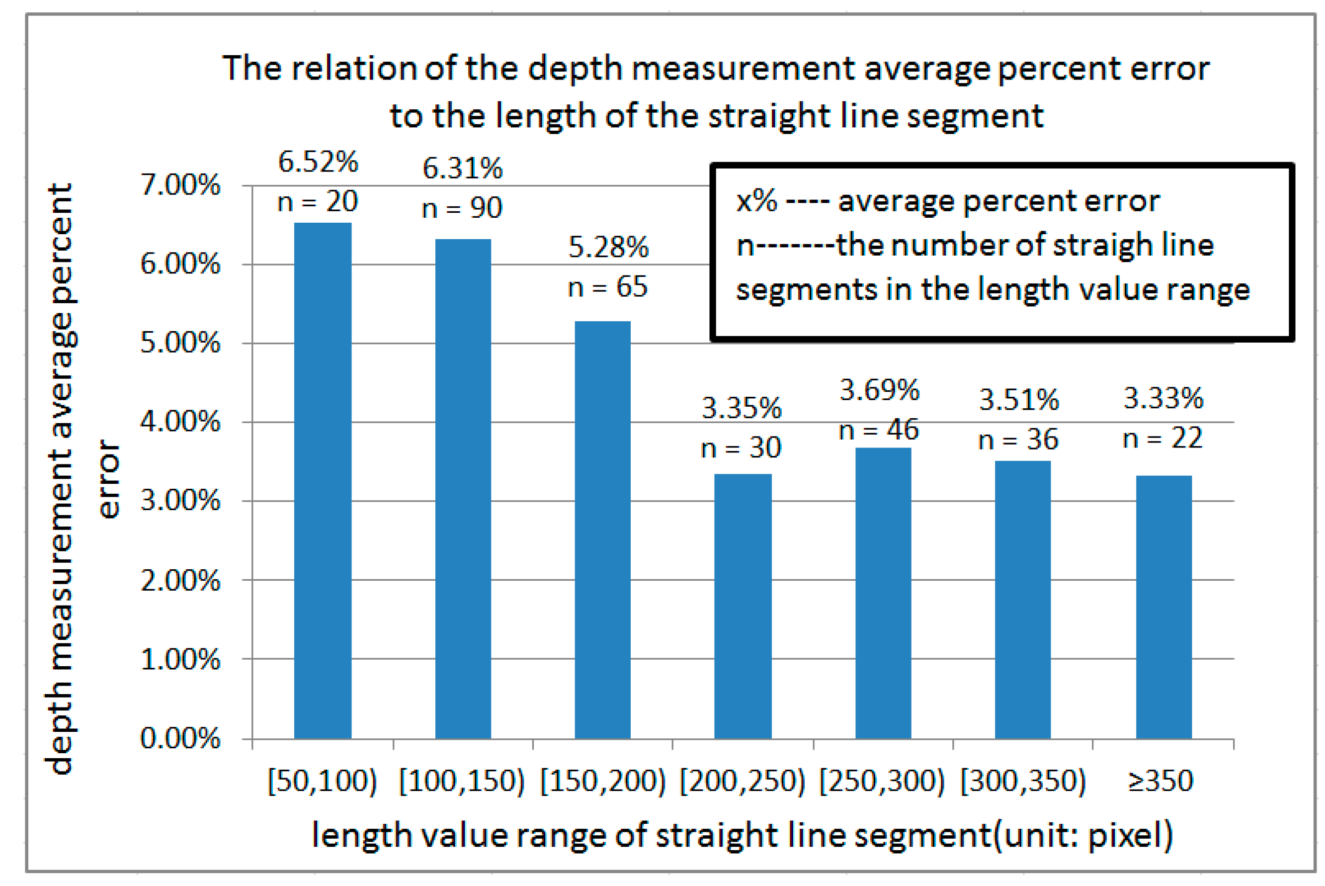
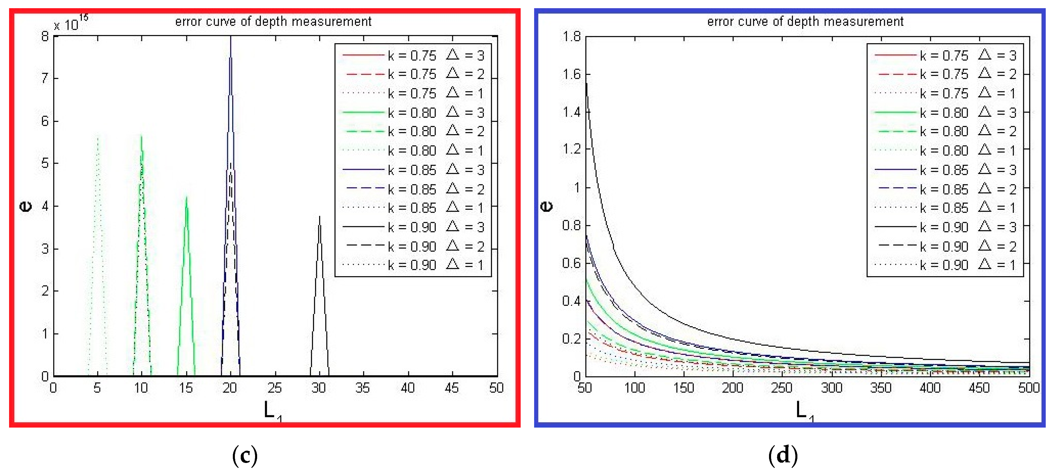
4.1. Theoretical Error Analysis

We can compute the depth of objects using Formula (3) if the length of the two straight line segments is known. In theory, the first straight line segment consists of any two SIFT feature points of an object in image A, and the second one consists of the two corresponding matching SIFT feature points in image B. There is always a certain error in the matching SIFT points, because the Nearest Neighbor Distance method is adopted to match the points. For example, we assume that the matching point of the SIFT feature point P_a in image A is theoretically the P_b in image B, but we get the matching point P_b′ in fact by the method. The distance between P_b and P_b′ is the error. Although, the error is very little, even no more than one pixel, the accuracy of estimating depth of object is dependent on it.

We assume the length of the straight line segment which consists of two SIFT feature points on an object in image A is L₁, and the length of the matching line segment is L₂ in image B, theoretically. But we obtain the length is L₂′ in fact for there are matching point errors. The difference between L₂ and L₂′ is Δ = L₂′ − L₂, and the relation of two length is L₂ = kL₁. We assume that U is ground truth of depth of object, and U′ is the computed depth of object by the Formula (3), and we have

$$U=\frac{L_2}{L_1-L_2}d$$

(6)

$$U\text{'}=\frac{L_2\text{'}}{L_1-L_2\text{'}}d=\frac{L_2+\Delta }{L_1-L_2-\Delta }d$$

(7)

$$e=\left|\frac{U\text{'}-U}{U}\right|=\left|\frac{\frac{\Delta }{1-k}}{L_1-\frac{\Delta }{1-k}}\right|\frac{1}{k}=\left|\frac{J}{L_1-J}\right|\frac{1}{k}$$

(8)

where e is percentage error of depth measurement, $J=\frac{\Delta }{1-k}$.

Normally, the ∆ is very little, no more than several pixels, even a single pixel, because ∆ is produced by the matching error of SIFT feature points. We assume |∆| ≤ 3 pixels, and 0.75 ≤ k ≤ 0.9, then 0 ≤ |J| ≤ 30. The Figure 3 shows the relations of e to k and ∆. Figure 3a shows the error curve when ∆ ≤ 0. Figure 3b shows the error curve when ∆ > 0. The range of e values was so large that the curve is hard to see when the L₁ more than 50 in Figure 3b, therefore, it was divided into two parts, as Figure 3c,d. From Figure 3 and Formula (8), we know: (1) that e increases rapidly when L₁ → J; and (2) that L₁ is longer, and e is lower, when the value of L₁ is higher than a certain value (e.g., 50) and the variable ∆ and k are unchanged. Hence we should select the longest straight line segment to compute the depth of object to minimize the error.

It is also proved by the experimental method that when the L₁ is longer, the error is smaller. In the experiment, we select the longest straight line segment, the shortest one, the middle length one, and a random one to compute the depth of object, respectively. 103 pairs of images (resolution: 1280 × 1024 pixels) were used, and the depth of 309 objects in the images were to be measured.

Table 1. Relation of depth measurement error to the 4 classes straight line segment (length unit: pixel).

Method	The Method of the Longest Line	The Method of the Shortest Line	The Method of the Middle Line	The Method of the Random Line
Length of the shortest line	50.19	0.15	21.29	2.31
Length of the longest line	481.61	22.81	362.41	377.35
Average length	205.71	3.01	91.25	95.59
Average error of measurement	4.89%	535.66%	20.57%	173.82%

shows the experimental results of the above 4 classes of straight line segment selected to measure depth. For every class of straight line segment, different objects have different lengths, so value range of the length of every class line segment is shown in Table 1. It indicates that we should select the longest straight line segment to compute the depth of object.

Different objects have different lengths of the longest straight line segment, which consists of the 2 SIFT points on the object. We counted the longest ones on the 309 objects and obtained the piecewise relations of depth measurement error to the length of straight line segment, as shown in Figure 4. It illustrates that the longer the straight line segment, the smaller the error; but the change in percentage error is very small when the length is greater than a certain number (e.g., 200). The experiment result coincides with the theoretical analysis of percentage error (Figure 3).

4.2. Decrease Time Complexity

In a 2-D plane, n points can form C(n,2) straight line segments. The time complexity is O(n²) if we compare a line segment length with others one by one to select the longest one. The amount of computation will increase sharply when the value of n is very large. Therefore, we must design an algorithm to cut down the computing time and find the longest line segment rapidly. The convex hull theory is employed to solve this problem.

If we assume that CH is a convex hull of a given points set Q, CH is defined as the unique minimal convex set containing Q. It implies all of the points in set Q must be in or on the boundary of convex hull CH. Therefore, If there are n points in the Q, then we can get C(n,2) straight line segments which consist of all the points. The two endpoints of the longest one must be on CH.

Convex hull of points set Q can be obtained by Graham scan. The time complexity of the method is O(nlgn). We assume that there are n points in the set Q, and m points among n belong to the convex hull of set Q. Thus we can find the longest straight line segment from the C(m,2) straight line segments instead of C(n,2) ones. In general, m $\ll$ n when n is a large number. It means we can decrease the computational complexity of seeking the longest straight line segment by using the convex hull.

4.3. Algorithm for Selecting a Pair of Straight Line Segments

As similarity measurement is employed to match SIFT feature points [23,24], the wrong matching points are sometimes chosen, although it is very rare. Even if only one of the endpoints of the pair of straight line segment that were used to compute the depth of object is wrongly matched, the value of depth measurement would be widely inaccurate. Hence, we should select the longest straight line segment whose two endpoints will be matched correctly to the corresponding SIFT feature points in image B.

Because images A and B are captured when the object distance is u and u + d, respectively, under the condition of keeping the camera’s intrinsic properties unchanged, we can use similarity of polygons consisting of the SIFT matching points on the image A and image B to tell whether the matching point is wrong or not. In our experiment the polygon is a triangle. In other words, if the triangle ∆ABC that consists of 3 SIFT feature points in image A is similar to the corresponding one ∆A’B’C’ in image B, then there are no wrong matching points in the three vertices. Otherwise, there is one wrong matching point at least.

The differences between every corresponding angle of the two triangles are employed to decide whether the two triangles are similar, and we call the maximal angle difference is Ang_max. If Ang_max < T_a, then the two triangles are similar. Where the T_a is a threshold.

The similarity of the triangle, one of whose sides is the longest line segment, should be determined; only in this way can we avoid the incorrect endpoints and minimize the error of depth measurement at the same time. It is impossible to determine which one or more vertices of triangle is/are the wrong matching point(s) when the triangle ∆ABC is not similar to ∆A’B’C’. Therefore, an algorithm for selecting a pair of straight line segments which are used to compute the depth is proposed. The main idea in the algorithm is as follows: we assume that the number of the triangles, one of whose sides is the longest straight line segment L, is n₁ in image A. Obviously, there are n₁ corresponding triangles in image B, but only n₂ pairs of triangles are similar. The L can be used to compute depth of object if n₂/n₁ > T_s, where T_s is a threshold. Otherwise, we should decide whether the next longest straight line segment is the one that we are seeking by the above method. The algorithm of selecting a pair of straight line segments is shown in the Algorithm 1.

Algorithm 1. The algorithm for selecting a pair of straight line segments.

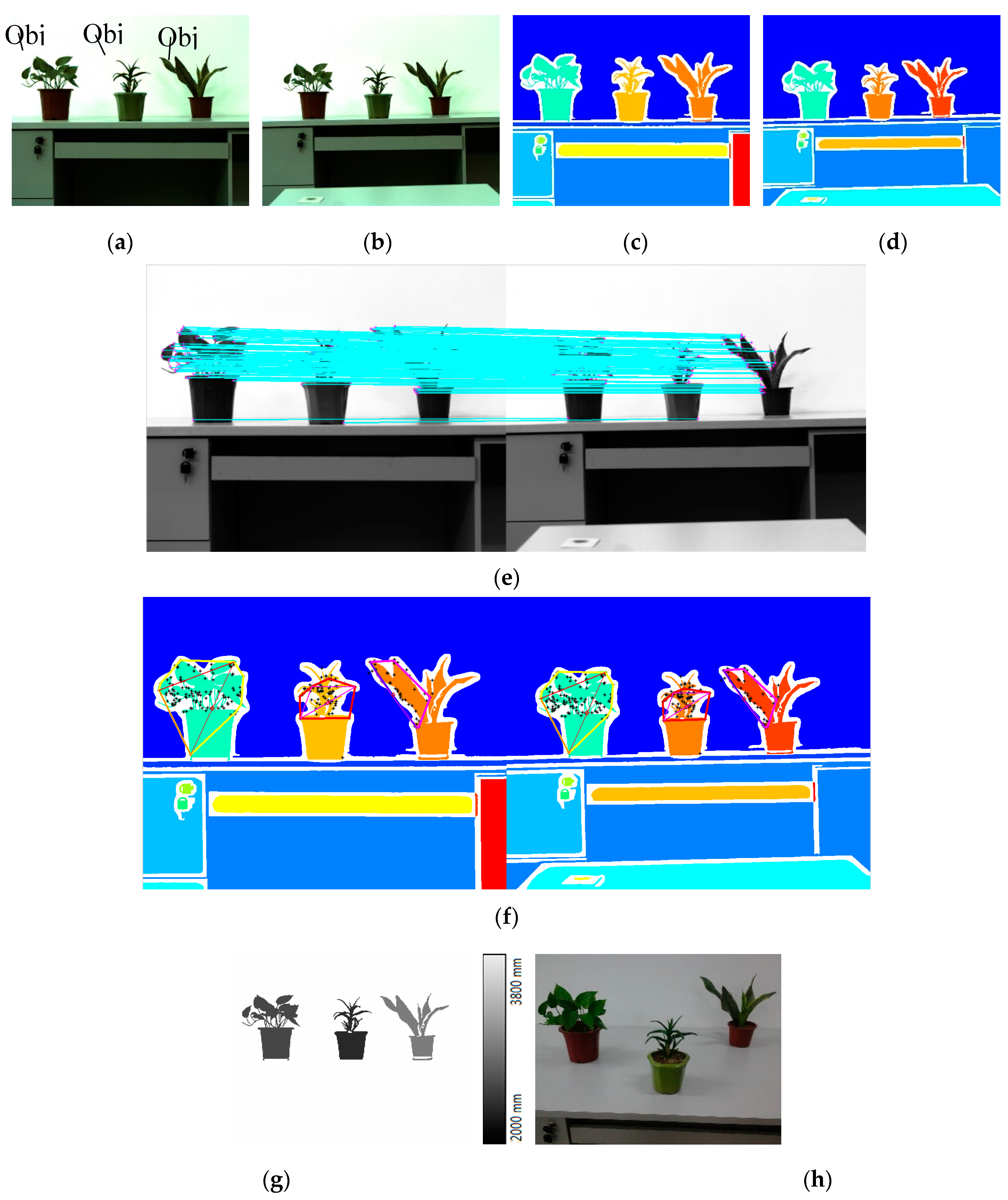
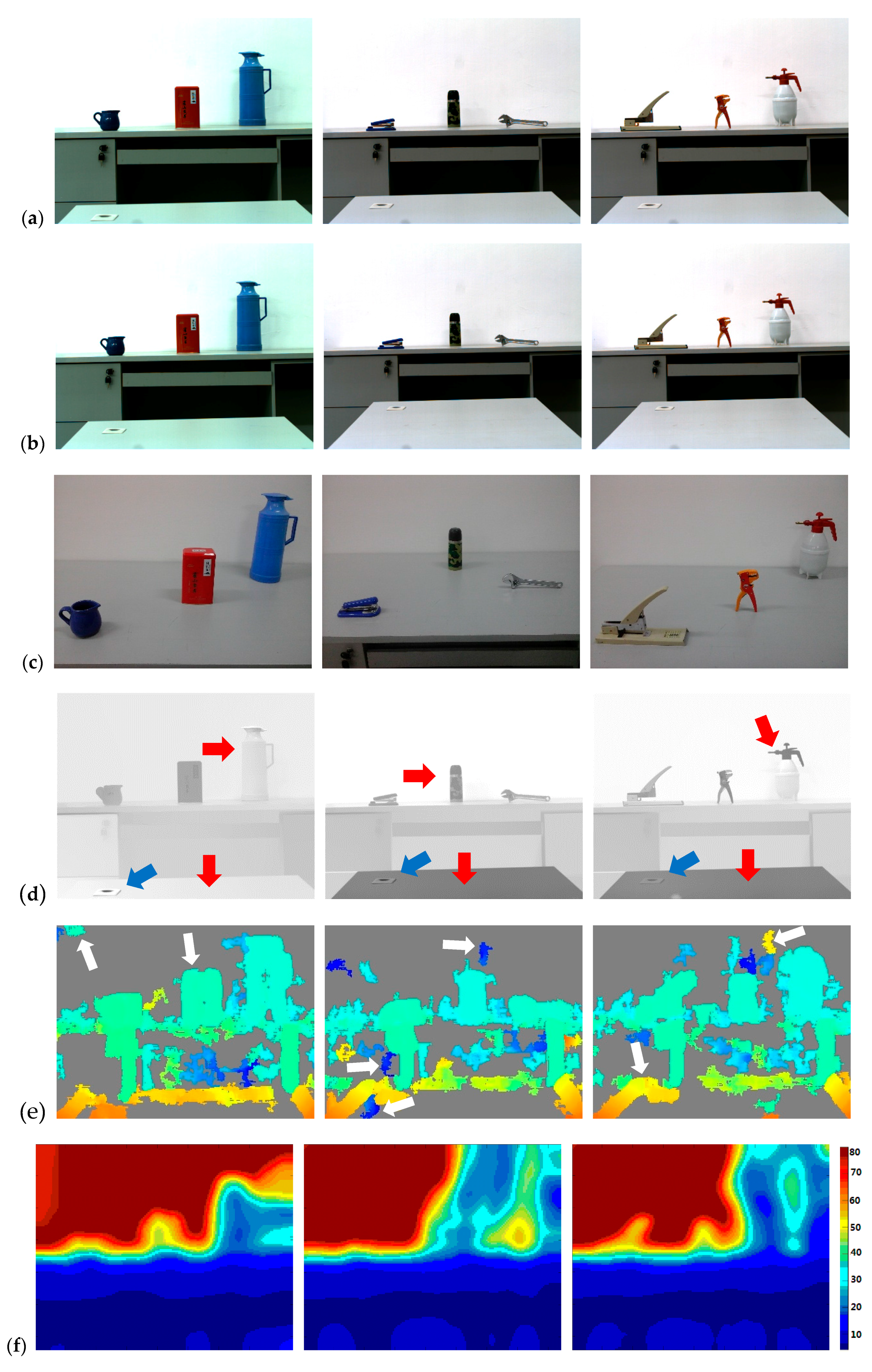
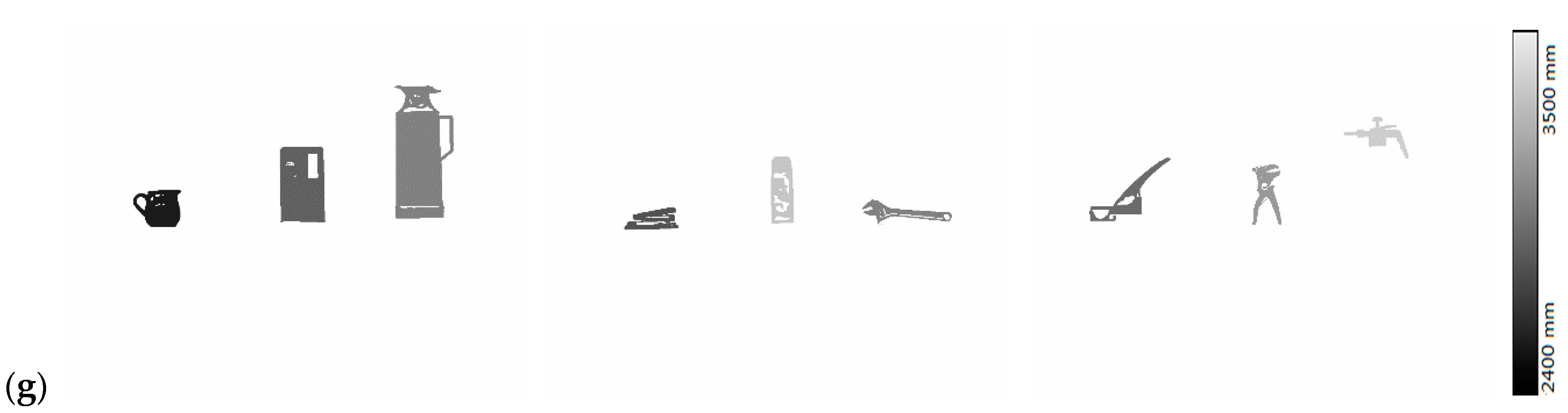
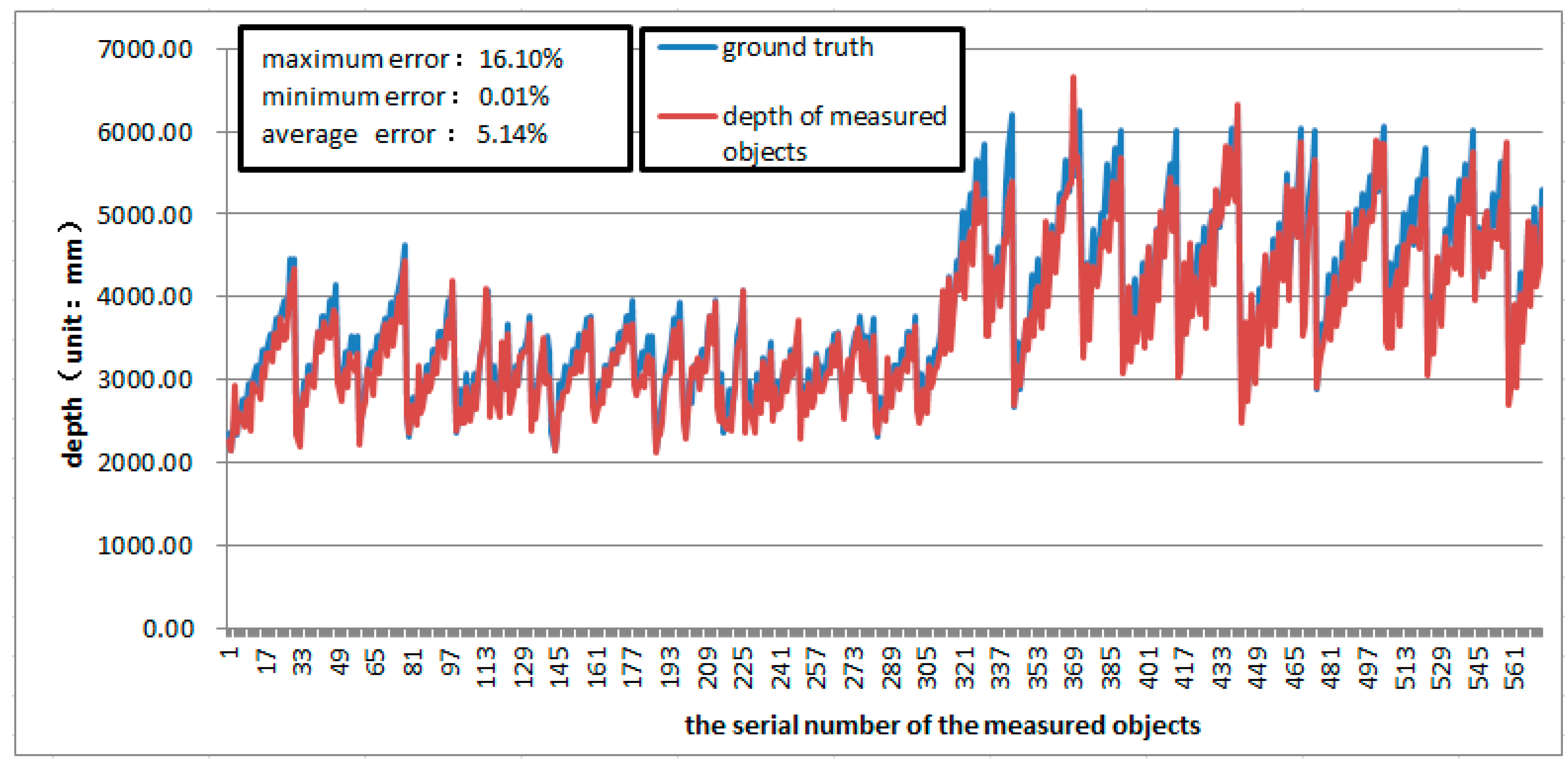
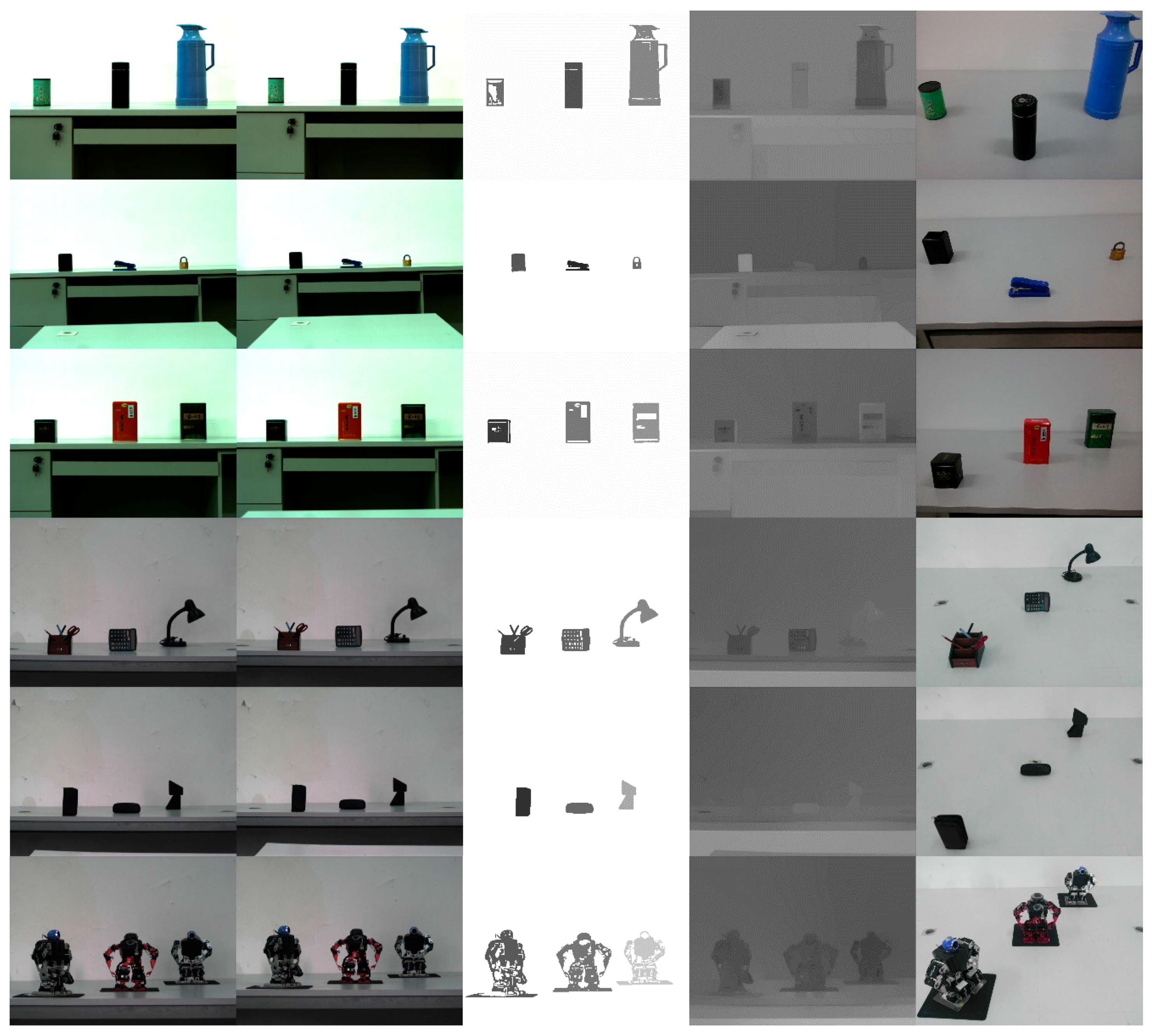
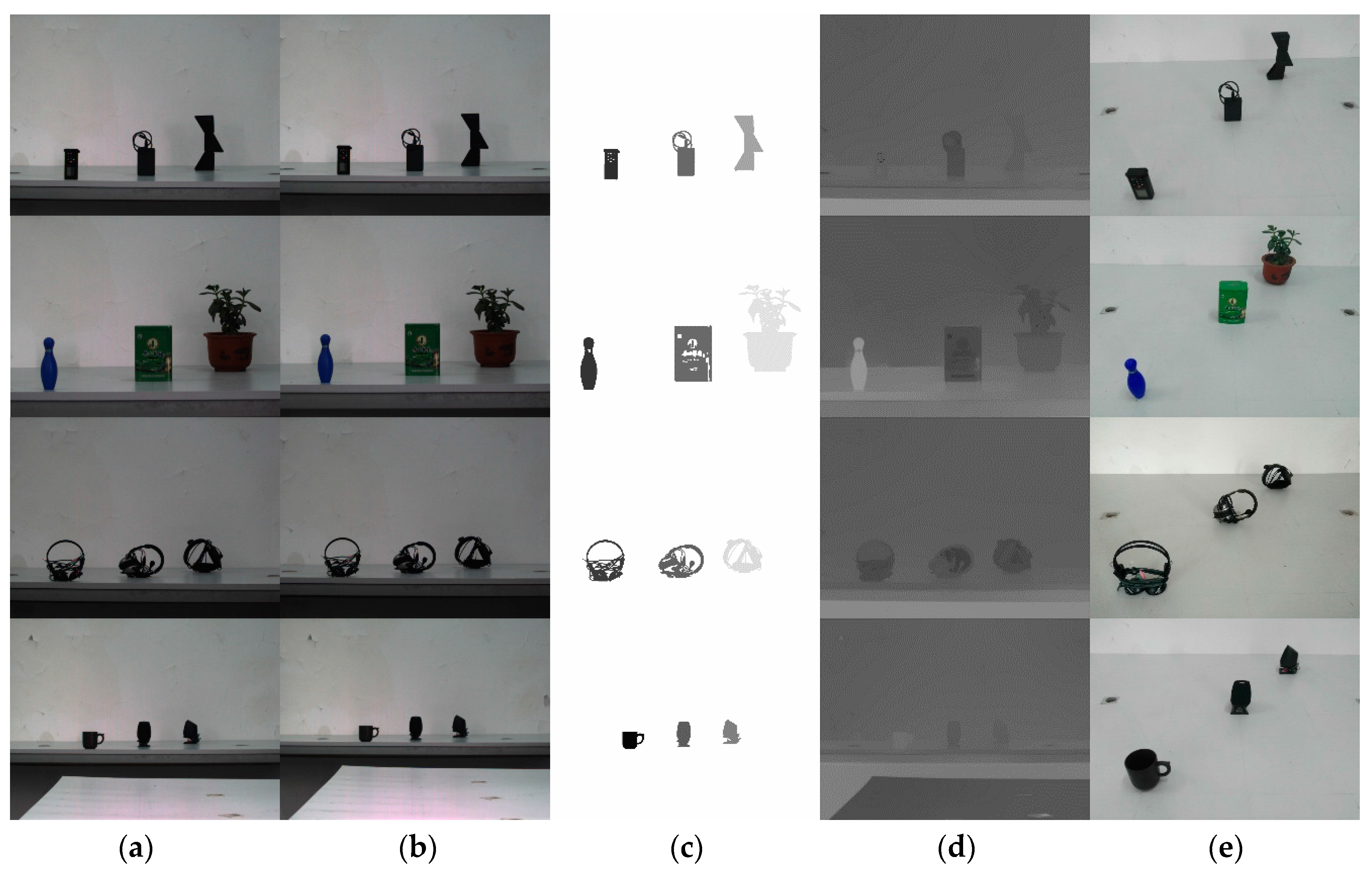
Input:  A sub-region in image A and its matched one in image B of the same object; The points set Q consists of the SIFT feature points of the object in image A, and in image B, the points set Q’ consists of the matched points of Q. Output:  A pair of straight line segments used to compute depth of object.

Step1: Assume i = 1. Step2: Compute to obtain the points set P, and the P is the convex hull of Q. Step3: Compute to obtain the length of all of the straight line segments which are composed of any 2 points in P, and put them in their length order, from the longest to the shortest. Step4: Count n1 and n2, where n1 is the number of triangles, one of whose side is the i-th longest line segment in image A, and n2 is the number of the corresponding and similar triangles in image B. Step5: If n2/n1 > Ts, go to step6; else, i = i + 1, and go to Step4. Step6: The i-th longest straight line segment in image A and the corresponding one in image B are the pair of straight line segments, which will be used to compute the depth of object.

Method 1 is used to compute the depth after the wrong matching points have been deleted by the above algorithm. Method 2 is used to compute the depth by the longest straight line segment directly. The measurement errors of the two kinds of methods are showed in

Table 2. Measure result comparison of the two kinds of methods (unit: distance—mm; length of line segment—pixel; angle—degree. D = 600 mm, T_a = 3°).

Object	GT 1	Method 1						Method 2
		Angmax	i-th 2	L1	L2	MD 3	EP 4	Lmax1	Lmax2	MD 3	EP 4
obj1	3565.38	0.35	1	269.00	229.34	3470.07	2.67%	269.00	229.34	3470.07	2.67%
obj2	3389.00	2.62	3	141.41	121.31	3620.50	6.83%	190.09	154.59	2612.66	22.91%
obj3	3758.01	0.55	1	302.35	257.87	3477.98	7.45%	302.35	257.87	3477.98	7.45%

¹ GT is the ground truth of the depth of object; ² the i-th means that the i-th longest straight line segment was used to compute the depth of object; ³ MD is measured depth; ⁴ EP is error percentage.

. There are 3 objects whose depth should be computed in the given images, and it is shown in Section 5.2. We called the 3 objects obj1, obj2, obj3, respectively. In method 2, the error percentage of depth measurement of obj2 is 22.91%, because 1 or 2 points of the two endpoints of the longest straight line segment are matched wrong. It is a very big error. But, in method 1, the error is decreased sharply, because the 3^rd-longest straight line segment was used to compute the depth of object by the above algorithm. Although its length is not the longest, it is the best choice to compute the depth information.

5. Experiments

5.1. Images Acquirement

To estimate the depth of objects in image, we must acquire two images (image A and image B). Figure 5 shows the process. Firstly, image A is acquired at the place where the distance between the object and the camera is u. Next, while the camera’s intrinsic properties remain unchanged, the camera is moved along the optical axis to the place where the object distance is u + d, and the image B is acquired. To obtain the actual distance of the objects, the objects to be measured were sitting at specified locations. In Figure 5a, the values of x₁, x₂, y₁, y₂, d and u can be obtained by using manual measurement; then, we can depend on the values, geometry and size of the objects to compute the actual depth of objects. For example, in Figure 5a, the object obj1 is a cylinder. Assume its diameter is D, then the actual depth of obj1 is ((u + y₂ + D/4)² + x₁²)^1/2. Similarly, the actual depth of obj2 and obj3 are u and ((u + y₁ + y₂)² + x₂²)^1/2, respectively.

Ordinarily, it is very difficult for the camera to move rigorously along the optical axis. In practical operation, the camera can be installed on a horizontal guide rail or platform on which a straight line has been drawn, with the camera then being moved along the guide rail or the straight line on the platform. This makes the moving direction approximately coincident with the optical axis. In our experiments, the camera is put on a horizontal platform which consists of several identical lab benches and moved along a straight line which had been drawn on the platform beforehand. The scene is showed in Figure 5b.

5.2. Experiment Procedure

To test and verify that our approach for depth measurement is effective, we acquire the images and follow the method steps to carry out experiments. Figure 6 illustrates the procedure for our approach. There are original images, the depth image of objects and some significant interim result images, etc., in Figure 6.

From Figure 6f, we can see that a whole image of measured objects is not necessary to measure the depth of object, because the depth can be computed by the lengths of a pair of straight line segments. And the pair of straight line segments can usually be obtained by a part of the image of the object. Consequently, our method is robust to occlusion or partial loss of image of object.

5.3. Our Approach Compared with Others’

We compare our experiment results with Bumblebee’s, Zhou’s [17] and Fang’s [20], as shown in Figure 7. There are three scenes, and different target objects measured are contained in each scene. Figure 7a,b contains images A and B, which are captured at different object distance by a common camera. The spatial relationships of the objects measured are shown in Figure 7c. The images are all taken from a top down view. They are convenient for us to estimate roughly whether a target object is near or far from the camera.

Figure 7d–g shows the depth images as measured by Zhou’s method [17], Bumblebee device, Fang’s method [20] and our method, respectively. In Figure 7d, Zhou gets dense depth maps, but they are relative depth information instead of absolute depth. Only depth of partial scenes are measured in Figure 7e,g, but they are absolute depth; namely they are object’s distance values, which are represented by different pixel values. Both the gray pixels in Figure 7e and the white pixels in Figure 7g indicate that the depth information of the place could not be measured. In Figure 7e–g, the different color or gray pixels mean different depth values.

There is some obviously incorrect depth information in Figure 7d. For example, in every image, the gray levels of the two objects which are indicated by red arrows are similar. It means that their depths as measured by Zhou’s method are similar, but, in fact, the disparity of the depth values is very big. The reason for this error is that Zhou’s method can only measure the defocus degree, and can’t judge the focal plane in front of or behind the imaging plane. Furthermore, the depth of the object which is indicated by blue arrows should be the same as its surroundings. But the results of the measurement are not consistent with the ground truth, because the texture of the image affects the construction accuracy of dense depth maps, which are obtained by applying matting Laplacian to perform sparse depth map interpolation [17].

We can also see that there are several obvious errors of depth measurement in Figure 7e, as the white arrows indicate. In fact, the depth values of the two places are very different, but the depth values measured by Bumblebee device are similar. So the colors of the two places are very similar in the images. In addition, the outlines of the objects in the depth images are different from the real objects. This was caused by error of measurement.

Figure 7f is the result of depth image by Fang’s method. The method is faster than the state-of-the-art method, and it can achieve quasi real-time performance. But the accuracy of depth information is not good. It is difficult for us to find the outlines of the objects from the depth image, especially the outlines of the small objects. In addition, the method needs a dataset to train and learn.

Figure 7g is result of depth image by our method. We can see that we can obtain a high accuracy in absolute depth of the target objects, and the outlines of the objects are clear and accurate in the depth images by our method. In Figure 7g, the depth of the watering pot head is shown, but the depth of the watering pot body cannot be measured, because the watering pot was divided into two parts—the watering pot head and the watering pot body after image segmentation—and not enough SIFT feature points could be detected on the watering pot body, due to the color of the body being very close to that of the background. Usually, if no less than 4 SIFT points are detected on an object, and then we can use them to compute the depth of objects. Therefore, our method works well in most cases.

Experiment images of the other ten scenes are showed in Figure 8. From left to right, each column is image A, image B, results of our method, results of the method of Zhou, and the rough spatial relationship of the measured objects, respectively.

In order to determine the degree of accuracy of result of our method, we took 191 group images for experiments. There are 382 images, for a group includes 2 images. And there are 3 target objects measured in a group, so 573 depths of objects should be measured. In our implementation, we used the same parameters for the whole experiment, i.e., T_p = 0.6, T_s = 0.6, T_θ = 3°. We compared the result of our method with the result of Kouskouridas et al.’s method [19], as shown in

Table 3. Comparison between our method with Kouskouridas et al.’s method [19].

Item Compared	Our Method	Kouskouridas et al.’s Method
Device required	camera	camera and laser depth measurement device
Number of images required	2	≥5 images for every measured object
Is a sample database required?	NO	YES
Can the depth of object which is not registered in the database be measured?	YES	NO
Average error percentage	5.14%	9.89%

.

In Kouskouridas et al.’s method, SIFT is employed to obtain the depth of objects, too. Firstly, a database needs to be built, and the measured objects must be registered in the database, or their depth cannot be measured. The database comprises object distance, a lot of images and their SIFT. The images of each measured object are taken from different object distances and different angles of view. A uniform and simple background is required in the images. The object distance is obtained by a laser device. Then, the data in the database is used for the training of their algorithm. For an image, the depth of the objects in the image can be computed only when the objects have been stored in the database. Above all, SIFT feature points should be detected. Then, the center of mass of feature points set and the average distance d_m between it and every feature point should be calculated. Lastly, the depth of objects can be computed by using d_m and some data in the database.

Table 3 shows advantages of our method include fewer devices, easy operation, no sample database, and less measurement error.

Figure 9 is the comparison of depth of the objects measured by our method with the ground truth. The horizontal axis represents the serial number of the measured objects. The vertical axis represents the depth of the measured objects. The red curve is the depth measured by our method, and the blue one is the ground truth, and. The maximum error is 16.1%, and the minimum error is 0.01%, and the average error is 5.14%. Figure 9 indicate that our method is effective.

6. Discussion

Firstly, image segmentation is employed in our approach. The accuracy of depth information of measured objects may be influenced by the result of image segmentation. It is not easy to separate the different types of objects measured from an image with a complex background using the same parameter. The depth accuracy would be reduced greatly if the result of segmentation is wrong. Therefore, how to extract the depth information of the target objects with complex background is one of our next works.

Secondly, our algorithm is time consuming, because image segmentation, SIFT feature point detection and matching are employed in our algorithm. The configuration of the computer which used to the experiment is as follows: memory 16 GB, CPU i7-4810MQ, 2.80 GHz, 4 cores. The codes were run in Matlab 2012b. It took about 139.6 s to extract the depth information from an image (resolution: 1280 × 1024 pixels) by our method. Of these, about 95 s were used for image segmentation, about 43.5 s were used for the SIFT feature point detection and feature point matching, and about 1.1 s were used for the rest. Therefore, we will focus on how to reduce the computational complexity in our next research.

Lastly, in our method, the images of the same object in the images A and B were matched by using SIFT feature points, and a pair of straight line segments, which were used to compute the depth of objects, were chosen according to the algorithm described in Section 4.3. When the length of the straight line segment was less than 150 pixels, shorter lengths of straight line segment correspond to lower accuracy of computed depth. Thus, our method has a low accuracy for very small objects. In addition, the depth cannot be measured unless there are no less than 4 SIFT feature points being detected on the target object. Therefore, our next research will focus on how to improve the depth measurement accuracy of small objects and how to measure the depth of target object whose number of SIFT feature points is less than 4.

7. Conclusions

A novel method for depth measurement is proposed in this paper, according to our analysis of related work by other researchers, and their shortcomings. Firstly, in our method, the required device is very economical and it is convenient to operate. Only two images of the same scene need to be provided in our method. The two images are captured by a camera. The camera is a common one and its price is usually cheap. The camera doesn’t need to be calibrated and no parameter needs to be adjusted during imaging. Secondly, our method obtains the absolute depth of object instead of the relative depth; and it is robust to occlusion or partial loss of object, because the depth can be computed by the lengths of a pair of straight line segments, and the pair of straight line segments can usually be obtained from a part of the image of the object. Lastly, the superiority of our method has been shown through comparisons with the methods of references [17,19,20] and the method of Bumblebee. The effectiveness and practicability of our method is proved by our experimental results.

References

1. Santos, D.G.; Fernandes, B.J. HAGR-D: A Novel Approach for Gesture Recognition with Depth Maps. Sensors 2015, 15, 28646–28664. [Google Scholar] [CrossRef] [PubMed]
2. Huang, H.C.; Hsieh, C.T. An Indoor Obstacle Detection System Using Depth Information and Region Growth. Sensors 2015, 15, 27116–27141. [Google Scholar] [CrossRef] [PubMed]
3. Hosni, A.; Rhemann, C. Fast Cost-Volume Filtering for Visual Correspondence and Beyond. IEEE Trans. Pattern Anal. Mach. Intell. 2013, 35, 504–511. [Google Scholar] [CrossRef] [PubMed]
4. Jiang, H.; Xiao, J.X. A Linear Approach to Matching Cuboids in RGBD Images. In Proceedings of the IEEE Conference on Computer Vision and Pattern Recognition (CVPR), Portland, OR, USA, 23–28 June 2013; pp. 2171–2178. [Google Scholar] [CrossRef]
5. De-Maeztu, L.; Mattoccia, S. Linear stereo matching. In Proceedings of the IEEE International Conference on Computer Vision (ICCV), Barcelona, Spain, 6–13 November 2011; pp. 1708–1715. [Google Scholar] [CrossRef]
6. Tao, M.W.; Hadap, S. Depth from Combining Defocus and Correspondence Using Light-Field Cameras. In Proceedings of the IEEE International Conference on Computer Vision (ICCV), Sydney, NSW, Australia, 1–8 December 2013; pp. 673–680. [Google Scholar] [CrossRef]
7. Chen, C.; Lin, H.T. Light Field Stereo Matching Using Bilateral Statistics of Surface Cameras. In Proceedings of the IEEE Conference on Computer Vision and Pattern Recognition (CVPR), Columbus, OH, USA, 23–28 June 2014; pp. 1518–1525. [Google Scholar] [CrossRef]
8. Tao, M.W.; Wang, T.C. Depth Estimation for Glossy Surfaces with Light-Field Cameras. In Proceedings of the European Conference on Computer Vision (ECCV), Zurich, Switzerland, 6–12 September 2014; pp. 533–547. [Google Scholar] [CrossRef]
9. Tao, M.W.; Su, J.C. Depth Estimation and Specular Removal for Glossy Surfaces Using Point and Line Consistency with Light-Field Cameras. IEEE Trans. Pattern Anal. Mach. Intell. 2016, 38, 1155–1169. [Google Scholar] [CrossRef] [PubMed]
10. Wang, T.C.; Efros, A.A. Depth Estimation with Occlusion Modeling Using Light-Field Cameras. IEEE Trans. Pattern Anal. Mach. Intell. 2016, 38, 2170–2181. [Google Scholar] [CrossRef] [PubMed]
11. Nayar, S.K.; Nakagawa, Y. Shape from Focus. IEEE Trans. Pattern Anal. Mach. Intell. 1994, 16, 824–831. [Google Scholar] [CrossRef]
12. Subbarao, M.; Tyan, J.K. Selecting the optimal focus measure for autofocusing and depth-from-focus. IEEE Trans. Pattern Anal. Mach. Intell. 1998, 20, 864–870. [Google Scholar] [CrossRef]
13. Pentland, A.P. A New Sense for Depth of Field. IEEE Trans. Pattern Anal. Mach. Intell. 1987, 9, 523–531. [Google Scholar] [CrossRef] [PubMed]
14. Subbarao, M.; Gurumoorthy, N. Depth recovery from blurred edges. In Proceedings of the IEEE Conference on Computer Vision and Pattern Recognition (CVPR), Ann Arbor, MI, USA, 5–9 June 1988; pp. 498–503. [Google Scholar] [CrossRef]
15. Rajagopalan, A.N.; Chaudhuri, S. Depth estimation and image restoration using defocused stereo pairs. IEEE Trans. Pattern Anal. Mach. Intell. 2004, 26, 1521–1525. [Google Scholar] [CrossRef] [PubMed]
16. Favaro, P.; Soatto, S. Shape from defocus via diffusion. IEEE Trans. Pattern Anal. Mach. Intell. 2008, 30, 518–531. [Google Scholar] [CrossRef] [PubMed]
17. Zhuo, S.J.; Sim, T. Defocus map estimation from a single image. Pattern Recogn. 2011, 44, 1852–1858. [Google Scholar] [CrossRef]
18. Zhou, C.; Nayar, S. What are good apertures for defocus deblurring? In Proceedings of the IEEE International Conference on Computational Photography (ICCP), San Francisco, CA, USA, 16–17 April 2009; pp. 1–8. [Google Scholar] [CrossRef]
19. Kouskouridas, R.; Gasteratos, A. Evaluation of two-part algorithms for objects’ depth estimation. IET Comput. Vis. 2012, 6, 70–78. [Google Scholar] [CrossRef]
20. Fang, S.; Jin, R.; Cao, Y. Fast depth estimation from single image using structured forest. In Proceedings of the IEEE International Conference on Image Processing (ICIP), Phoenix, AZ, USA, 25–28 September 2016; pp. 4022–4026. [Google Scholar] [CrossRef]
21. Li, C.M.; Kao, C.Y. Implicit active contours driven by local binary fitting energy. In Proceedings of the IEEE Conference on Computer Vision and Pattern Recognition (CVPR), Minneapolis, MN, USA, 17–22 June 2007; pp. 339–345. [Google Scholar]
22. Li, C.M.; Kao, C.Y. Minimization of region-scalable fitting energy for image segmentation. IEEE Trans. Image Process. 2008, 17, 1940–1949. [Google Scholar] [CrossRef] [PubMed]
23. Lowe, D.G. Distinctive image features from scale-invariant keypoints. Int. J. Comput. Vis. 2004, 60, 91–110. [Google Scholar] [CrossRef]
24. Lowe, D.G. Object recognition from local scale-invariant features. In Proceedings of the Seventh IEEE International Conference on Computer Vision (ICCV), Kerkyra, Greece, 20–27 September 1999; pp. 1150–1157. [Google Scholar] [CrossRef]
Figure 1. Two times imaging of lens. D is the diameter of the camera aperture. V’ is the distance between the camera lens and the image plane. S1 and S2 are the same point S on the imaging object SL. In the first imaging, the object distance is u, and the imaging object SL is located at S1L1, and the S1’ is the focal point of S. In the second imaging, the object distance is u + d, and the imaging object SL is located at S2L2, and the S2’ is the focal point of S.
Applsci 07 00517 g001
Figure 2. The overview of our depth measurement method.
Applsci 07 00517 g002
Figure 3. Relation of depth measurement error to the length of straight line segment L1. (a) Error curve when ∆ ≤ 0; (b) Error curve when ∆ > 0. In order to clearer, this graph is separated into two parts, namely the red part and the blue part. They are showed in (c) and (d), respectively; (c) Error curve when L1 [0,50] and ∆ > 0, namely this is the red part of figure (b); (d) Error curve when L1 [50,500] and ∆ > 0, namely this is the blue part of figure (b).
Applsci 07 00517 g003aApplsci 07 00517 g003b
Figure 4. Experimental results of the relation of the depth measurement average percent error to the length of the straight line segment.
Applsci 07 00517 g004
Figure 5. (a) is the schematic diagram of the process acquiring the two images; (b) is the real scene which was used to capture the image A and B.
Applsci 07 00517 g005
Figure 6. The experimental procedure. (a) The original image A was acquired at the place where the object distance is u; (b) the original image B was acquired at the place where the object distance is u + d; (c) and (d) are the segment results of the image (a) and (b), respectively. In order to make the sub-regions clear, we label the different sub-regions with different colors; (e) SIFT feature points detected and matched. The true-color image A and B are converted to grayscale; then, detect the SIFT feature points in them, and match the points. The locations with a pink star “*” are the locations of SIFT feature points; (f) matching the objects by taking advantage of the SIFT feature points and the segment results. Then we get the convex hull of the set of SIFT feature points of each object to be measured by Graham scan. Lastly, the pair of straight line segments are chosen by the algorithm described in Section 4.3. They are labeled by drawing a sign “◇” on it; (g) the depths of objects are expressed by the gray-scale. The gray value of pixel is lower, the value of depth is lower, too; (h) this image shows the spatial relationship of the objects. Namely, there are the different distances between camera and the different measured objects. It is convenient for us to compare with image (g).
Applsci 07 00517 g006
Figure 7. Comparison of depth estimation results of different approaches. (a)This row contains the original images A taken by a common camera; (b) this row contains the original images B taken by the same camera, only the object distance is different; (c) this row of images, which are taken from a top down view, show the space relationship of measured objects. They are convenient for us to judge if an object is near or far from the camera, roughly; (d) this row contains the depth images as measured by the Bumblebee device; (e) this row contains the depth maps that measured by the method of Zhou [17]; (f) this row contains the depth maps that measured by the method of Fang [20]. The source code is available on GitHub (https://github.com/king9014/rf-depth); (g) this row contains the depth images that measured by our method.
Applsci 07 00517 g007aApplsci 07 00517 g007b
Figure 8. The experiment images of the ten scenes. The column (a) contains the original images A. The column (b) contains the original images B. The column (c) contains the depth images that were measured by our method. The column (d) contains the depth images that measured by the method of Zhou [17]. The column (e) images, which are taken from a top down view, show the spatial relationship of the measured objects. They are convenient for us to judge if an object is near or far from the camera, roughly.
Applsci 07 00517 g008aApplsci 07 00517 g008b
Figure 9. Comparison the depth of the objects measured by our method with the ground truth.
Applsci 07 00517 g009