Variability of Hydroacoustic Noise Probability Density Function at the Output of Automatic Gain Control System


Department of Instrument Engineering, Far Eastern Federal University, 690650 Vladivostk, Russia
*
Author to whom correspondence should be addressed.
Appl. Sci. 2018, 8(1), 142; https://doi.org/10.3390/app8010142
Submission received: 28 October 2017
/
Revised: 20 December 2017
/
Accepted: 9 January 2018
/
Published: 20 January 2018
(This article belongs to the Special Issue Underwater Acoustics, Communications and Information Processing)
Abstract
:This research presents results of the estimation of temporal variability of the hydroacoustic noise probability density function (PDF) in shallow waters within the frequency band of 0.03–3.3 kHz; the studies were conducted near the Primorsky Aquarium on Russky Island, Vladivostok, Russia. Signals were received via unidirectional hydrophone and automatic gain control of the received signals. The hydrophone was attached to a drifting buoy via an elastic suspension; the received signals were transmitted by cable to a boat drifting with the buoy. The results of the comparison of the sea noise probability density function (PDF) estimates at the output of a system with automatic gain control (AGC) with similar results for a white Gaussian noise in the same frequency band are described.
1. Introduction
Today, the examination of technical conditions, photo- and video shooting of underwater cables, pipelines, and engineering structures is conducted via autonomous underwater vehicles (AUVs) along with traditional diving means; control and communication with AUVs are usually established through a hydroacoustic communication channel. One of the limiting factors for the characteristics of hydroacoustic communication is the underwater noise of natural and anthropogenic origins. It may be caused by water noise, seismic noise, flow noise, activities of the shipping industry, as well as activities of industrial and transportation enterprises located at the shelf, on the shore, and nearby the shore.
For the appropriate consideration of influences of the underwater nonstationary noise on the characteristics of hydroacoustic communication systems, it is essential to obtain knowledge of its mathematical and physical models at time intervals that are comparable with durations of used signals throughout the connection session. The duration of a connection session with continuous exchange of information with an AUV can be several hours or longer.
The distinctive peculiarity of the underwater noise that is observed in coastal areas with highly intensive shipping traffic is its prominent additional “short-time” nonstationarity; it becomes noticeable over time intervals that exceed a few dozen seconds. Therefore, it obstructs the forecasting of expected characteristics of the underwater noise, and consequently clouds the characteristics of hydroacoustic communication systems.
The use of mean nonstationary noise characteristics at time intervals that exceed 30 s, as well as data that was received in other coastal water areas with similar hydroacoustic conditions, cannot always be justified from the physical point of view.
Therefore, in order to evaluate the characteristics of hydroacoustic communication in a given water area, it appears viable to conduct long-term monitoring of underwater noise characteristics, accumulation, and generalization of statistical data.
Moreover, underwater noise caused by shipping and industrial activities at the sea shelf may have a negative effect on marine species. A number of national and international documents include characteristics of underwater noise in the list of monitored characteristics of coastal territories [1,2,3]. Recommended methods of measuring the sea noise parameters are described in [2,3,4]. Noise monitoring can be conducted for various purposes; therefore, the controlled parameters should be chosen accordingly.
For the purposes of underwater noise monitoring, specialized stationary systems (mounted to the sea floor and not intended for relocation), autonomous and drifting oceanological measuring systems that are intended for single use and multiuse, as well as the systems that are designed for taking measurements from the board of a moving or drifting vessel, can be used. In this case there are potential options of recording measurement information with built-in digital storage drives and/or life-stream of information via radio channel or cable.
This research shows some of the pilot results of estimating the time variability of one-dimensional probability density function (1-D PDF) acoustic pressure sample values of underwater noise in the Peter the Great Bay, Sea of Japan, in the area east of the Primorsky aquarium, which is located on Russky Island, Russia. The method of histograms was used to evaluate PDFs. Knowing how the PDF of noise changes over time (for instance, when the vessel is passing by) allows more precise estimation of the likelihood ratio and implementation of the adaptive and robust signal detection algorithms.
2. Materials and Methods
The depth in the research area is 30 m; the floor is sand; distance to the shore is 1 nautical mile. Approximately 2 nautical miles away from the research area there is an anchorage and water border of the outer aquatic area of the port of Vladivostok; additionally, there is a route that is used for the entrance and exit of oceanic vessels in and out of the port. The given area is characterized by high shipping intensity; on average, vessels pass through this route every two hours.
The research was conducted in September–October 2014 in conditions of dry and calm weather; the mean wave height was 0.5 m. The distance from the research area to the nearby anchored vessels at that time was about 3 nautical miles. The current velocity did not exceed 0.1 m/s. The omnidirectional piezoceramic spherical hydrophone was 50 mm in diameter, with medium sensitivity of 180 μV/Pa within the frequency range of 0.03–4 kHz (constructive elements are considered); it was mounted to the drift buoy with flexible suspension and was used for the signal reception. Submersion depth of the hydrophone was 10 m. Signals received through the hydrophone were transferred to the boat with a water displacement of 3 metric tons via cable with attached floaters; the boat was drifting along with the buoy. The regime of silence was maintained onboard during the measurements; the equipment was powered by accumulator batteries.
A Brüel & Kjær Charge Amplifier Type 2635 (Brüel & Kjær, Naerum, Denmark) with input impedance of 1 GOhm was used as a hydrophone preamplifier. High-grade 24-bit external sound card E-MU 0404 USB2 (Creative Technology Ltd, Jurong East, Singapore) was used for signal sampling; the sampling frequency (fs) was 8 kHz. The digitized signals were recorded on a computer hard drive as *.wav files and then computer-processed in laboratory conditions. Some spectral and statistical characteristics of the sea noise in the research area were described in [5,6].
In order to reduce the influence of low-frequency flow noise and noise with frequency components that exceed the Nyquist frequency (4 kHz in the given case) prior to further processing, signals were filtered by the 1024th-order finite-impulse-response filter with frequency bandwidth 30–3300 Hz.
3. Results
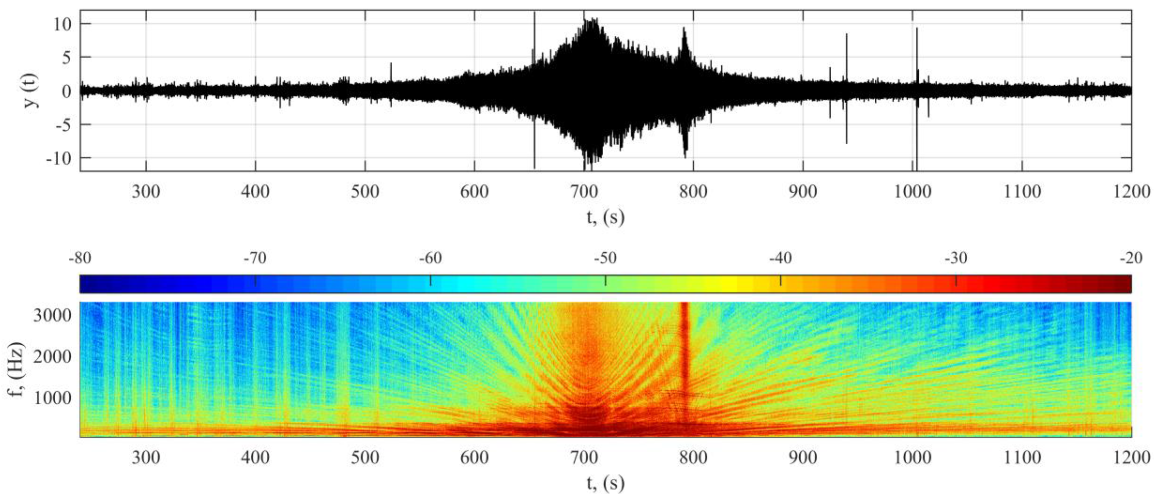
One of the most frequently occurring and usually most harmful components of underwater noise in shallow coastal water areas is the nonstationary noise caused by moving and anchoring vessels and motor boats. An oscillogram of a 16-min fragment of non-standardized signal at the hydrophone preamplifier output is shown in Figure 1, top; the vertical axis scale is conventional.
The oscillogram looks like a noise track with sharp and smooth maximums and peaks. Its images may be considered typical for the given region; the mean level of noise track depends generally on the state of the sea.
There is a smooth increase, maximum noise level around 710 s, and a smooth decrease afterwards—all caused by the passage of a cargo vessel with water displacement of approximately 800 metric tons and over 2 m draft (approach–departure) at a distance of about 0.3–0.5 nautical miles from the buoy that the hydrophone was mounted to.
The sharp increase in noise level in the area of 790 s was caused by a passing motor boat at the distance of about 0.1 nautical miles from the buoy. Barely noticeable in this scale maximums in the areas before 500 s and past 900 s comply with the passages of vessels at distances of over 3 miles. The short peaks on the oscillogram are caused by the abrupt movements of the flexible mount of the hydrophone which are inevitable in rough sea surfaces; the cable connects the buoy and the boat. Peaks at the time intervals of 650–820 s are caused by hitches of the elastic suspension and the cable, which were observed when there were surface waves, caused by movement of the vessel and motor boat.
Figure 1 (bottom) is a spectrogram (fast Fourier transform (FFT) size 1024, Hann window) of the signal and scale that reflect the dependency of color on the levels of spectral components of the signal in dB; the scale is conventional. Spreading in a fan-like shape, slope lines on the spectrogram physically represent an interference pattern changing over time, typical for the moving source of radiation in a hydroacoustic waveguide [7,8]. When listening to the signal, one can hear clicks at the time interval that corresponds to the minimum distance of the passing vessel; these clicks are caused by the propeller cavitation.
The character of the spectrograms is typical for the waveguide propagation of sound with damping of modes at frequencies below the critical value (cutoff frequency). The cutoff frequency f0 can be calculated using the following formula [8]:
This formula is exact only for a homogeneous water layer of depth D and sound speed cw overlying a homogeneous bottom of sound speed cb. For the depth D = 30 m, assuming cw = 1500 m/s and cb = 1600 m/s (sand and silt), the cutoff frequency is f0 = 33 Hz.
Changes not only in levels, but also in spectral content of the noise over time bring additional complications to the problem of the hydroacoustic signal detection. On a number of occasions, methods of automatic gain control (AGC) and normalization of the signal according to the required level are used in receiving devices of radio- and hydroacoustic communication the for the purposes of decreasing the dynamic range and stabilization of the terminal signal and noise levels. There are many methods of AGC implementation in analog and digital signal processing.
If the stationary random process can be used as a model of noise, then AGC is usually necessary to maintain the received signal at a constant signal strength. The statistic theory of AGC for this particular case is developed; its conclusions are widely used in practice. If the stationary random process cannot be used as the model, then in case of the nearby passage of a vessel or a motor boat with distinct propeller cavitation, when the levels of noise change at intervals of about a few minutes by over 20 dB or more (see Figure 1), AGC can be used for “stationarization” of the noise. The choice of time constant for AGC system (in this research it is equal to 1 s and does not change over time) is determined by the duration of the expected signals and noises. Since AGC is not a non-linear mathematical operation, it is difficult to forecast changes of PDF at the output of the AGC system. Therefore, the experimental estimation of PDF at the output of the AGC system in real conditions is of high interest.
During this research, AGC was implemented through the division of all signal sample values by corresponding values of signal “quasi-envelope”. “Quasi-envelope” values were obtained via the square law detection method. For the ease of further analysis, after the application of AGC, the signal was normalized by the levels in such a way that its sample mean value my and sample variance sy2 were 0 ± 0.0001 and 1 ± 0.0001, accordingly (bringing to the level (0, 1)).
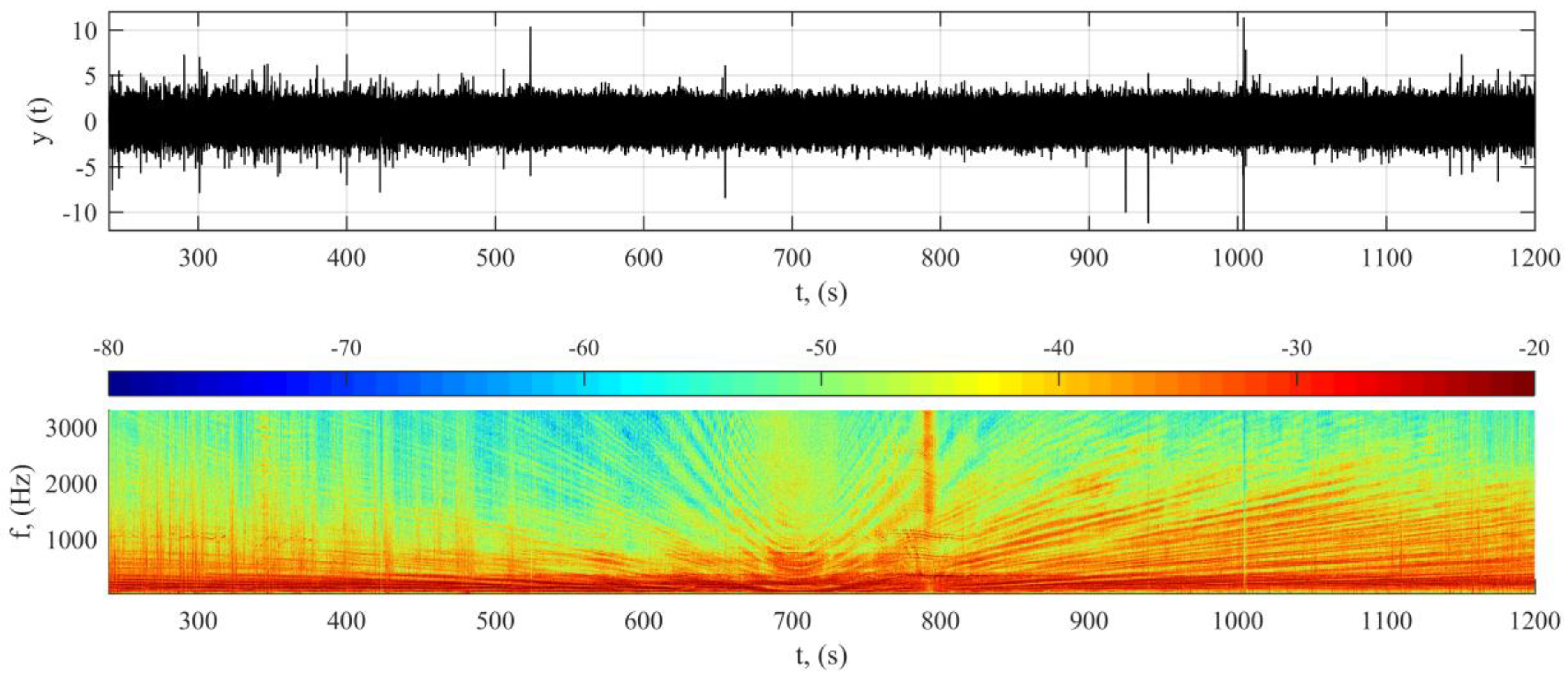
Figure 2 (top) represents an oscillogram of the same signal (as in Figure 1) after AGC and normalization; the vertical axis scale is conventional. The oscillogram looks like a noise track without smooth maximums caused by the vessel and the motor boat.
In Figure 2 (bottom), there is a spectrogram (FFT size 1024, Hann window) of the signal in Figure 2 (top). Above the spectrogram, there is a scale which reflects the dependency of color on the levels of spectral components of the signal in dB; the scale is conventional. The interferential pattern in the spectrogram became less noticeable; low-frequency components became more visible. For the description of the signal after AGC and normalization, a model of quasi-stationary ergodic random process of second order with my = 0 and sy2 = 1 can be already used as an initial approach.
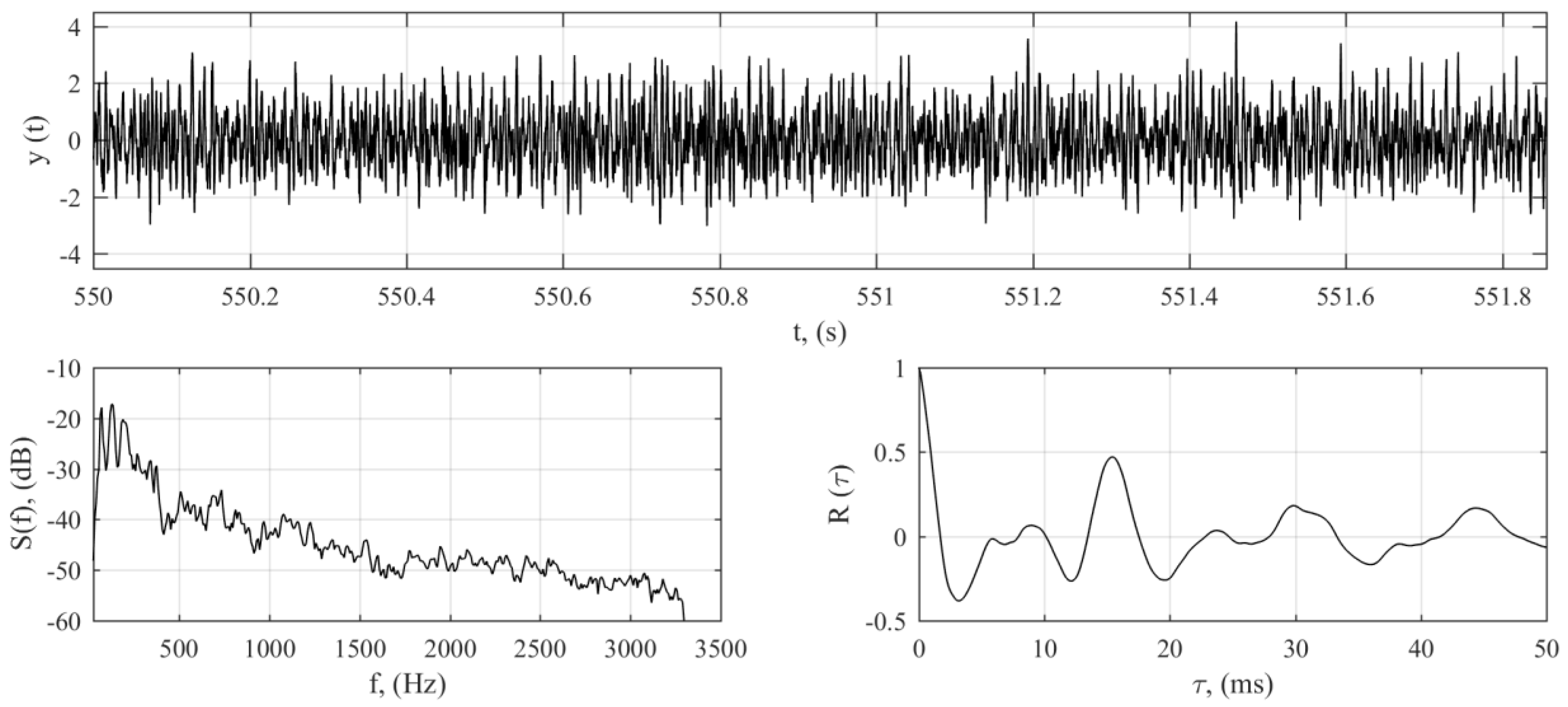
Figure 3 shows the oscillogram of the more detailed signal fragment, estimation of the mean spectrum (FFT size 1024, Hann window), and estimation of the initial area of the time correlation function of given signal after AGC and normalization for the time interval of 550–552 s. The spectrum has a slope typical for underwater noise and smoothed peaks at the frequencies lower than 100 Hz; the vibration of ship engines causes these peaks. The same peaks also represent the extremes of the time correlation function.
When it comes to estimation of the characteristics of an underwater communication system in real conditions, the evaluation of time variability of the PDF of statistically dependent (see correlation function in Figure 3) sampled values of underwater noise is an important problem. Some results of the experimental evaluation of the probability density of various noises are described in [8,9,10]. Theoretical aspects regarding the evaluation of probability density function according to the research data are described in [11,12,13]. In numerous papers it is assumed that the probability density distribution of sea noise is Gaussian.
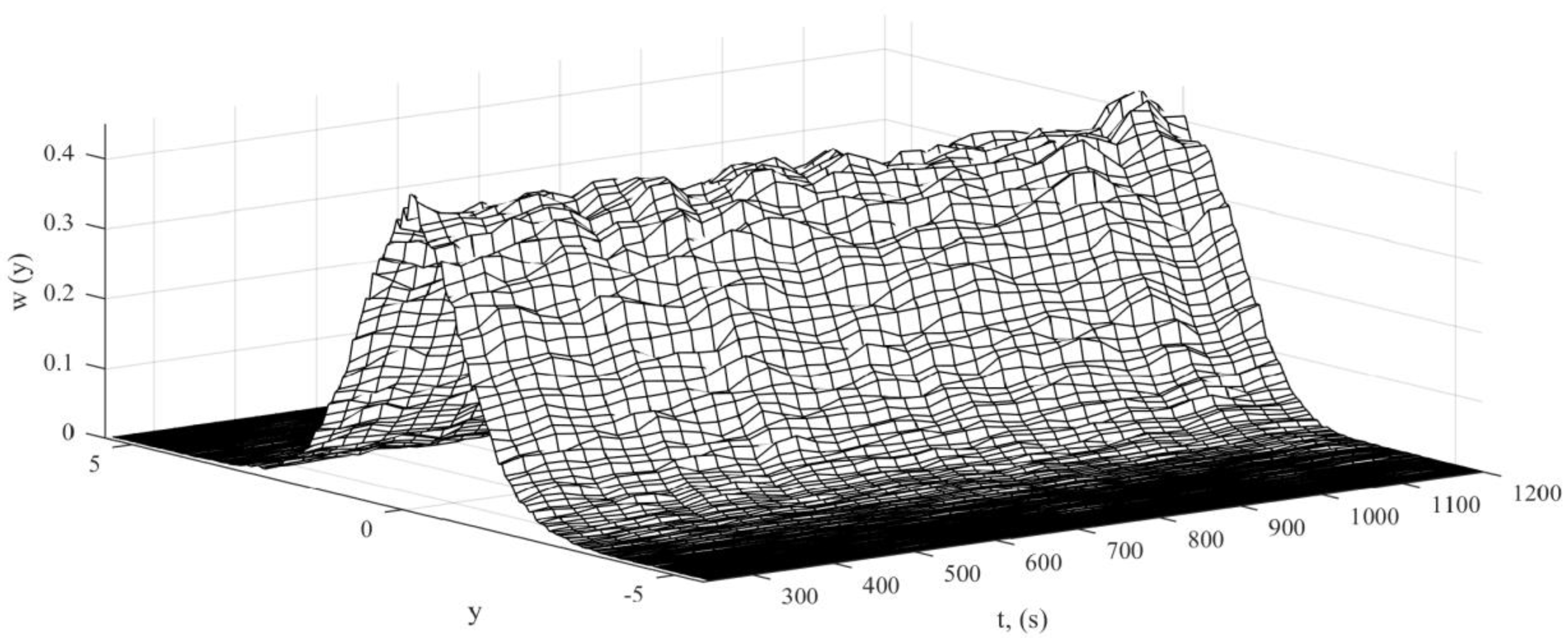
Figure 4 illustrates the estimation of time dependences of PDF w(y) for sampled values of the signal, shown in Figure 2 (top).
The histogram method of overlapping consecutive signal fragments by 50%, T = 10 s length each, (i.e., for consecutive fs × T = 8000 × 10 = 80,000 dependent samples) was used for the estimation of the PDF. The majority of smoothed histograms shown in Figure 4 are visually similar to the Gaussian curve with the mean equal to 0 and variance equal to 1. Nevertheless, neither checking for normality with significance level of 0.05 via application of the chi-square and Kolmogorov’s criteria [11,12,13,14] to the noise signal fragments that are shifting in time (30 min limit applies) nor changing accumulation time T from 0.1 s to 10 min have produced stable positive results. This could have been caused by ship traffic out of the line of sight, the anchorage, and the proximity of the port.
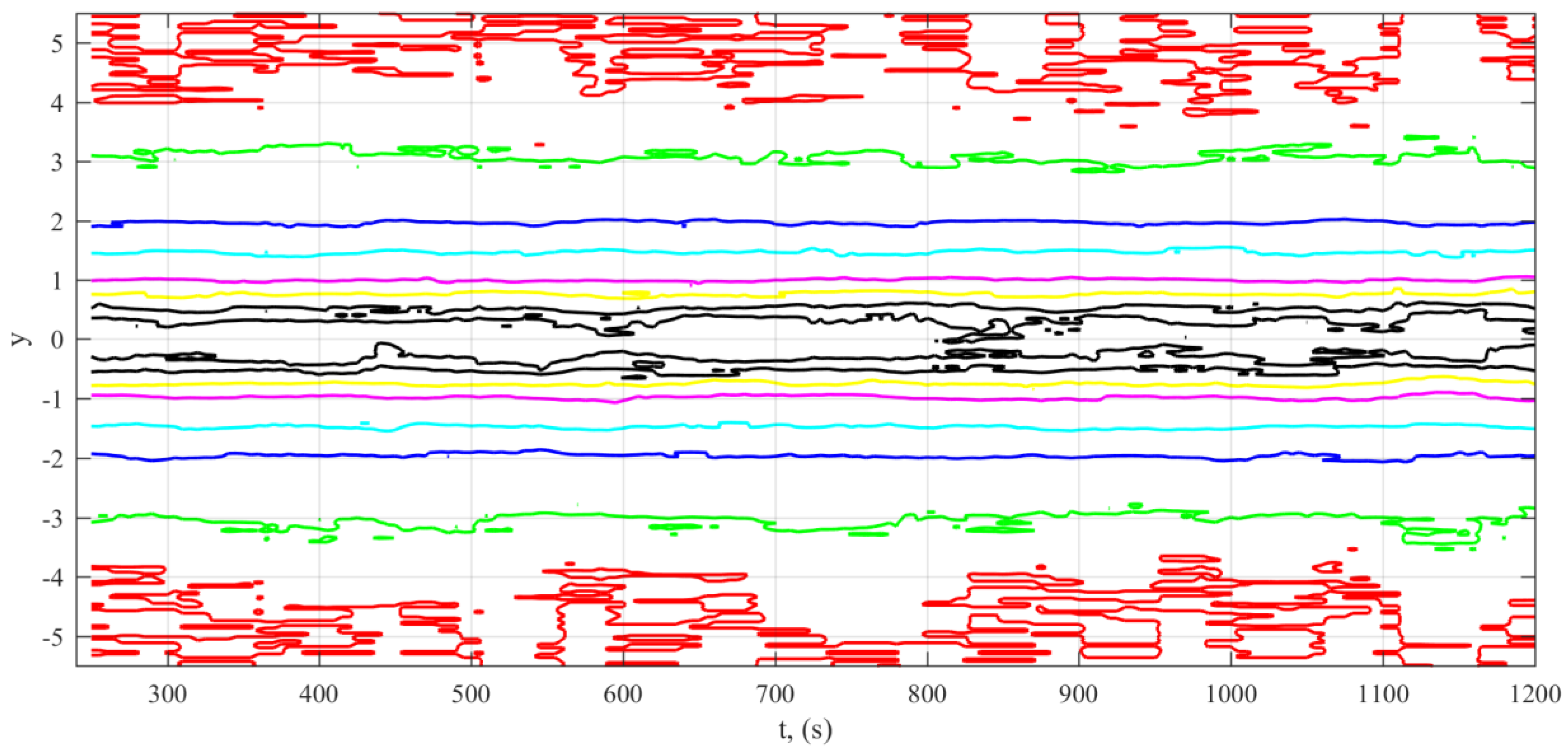
Figure 5 shows lines of equal probability of the values of w(y): 0.000134 (red), 0.004432 (green), 0.053991 (blue), 0.1295 (cyan), 0.241971 (magenta), 0.3521 (yellow), 0.3867 (black); the values are respective to the Figure 4. For the Gaussian distribution with the mean equal to 0 and variance equal to 1, this would be corresponding to the straight lines—also in accordance with values of y: ±4, ±3, ±2, ±1.5, ±1, ±0.5, ±0.25 [14].
It is shown in Figure 5 that with this duration of signal fragments, the major deviations from the Gaussian distribution are observed in the areas with |y| < 0.5 (area of the most probable sample values) and |y| > 3 (area of the least probable sample values) [14]. With this accumulation time, no changes resulting from the passage of either the vessel or the motor boat were observed (710 s and 790 s, see Figure 1).
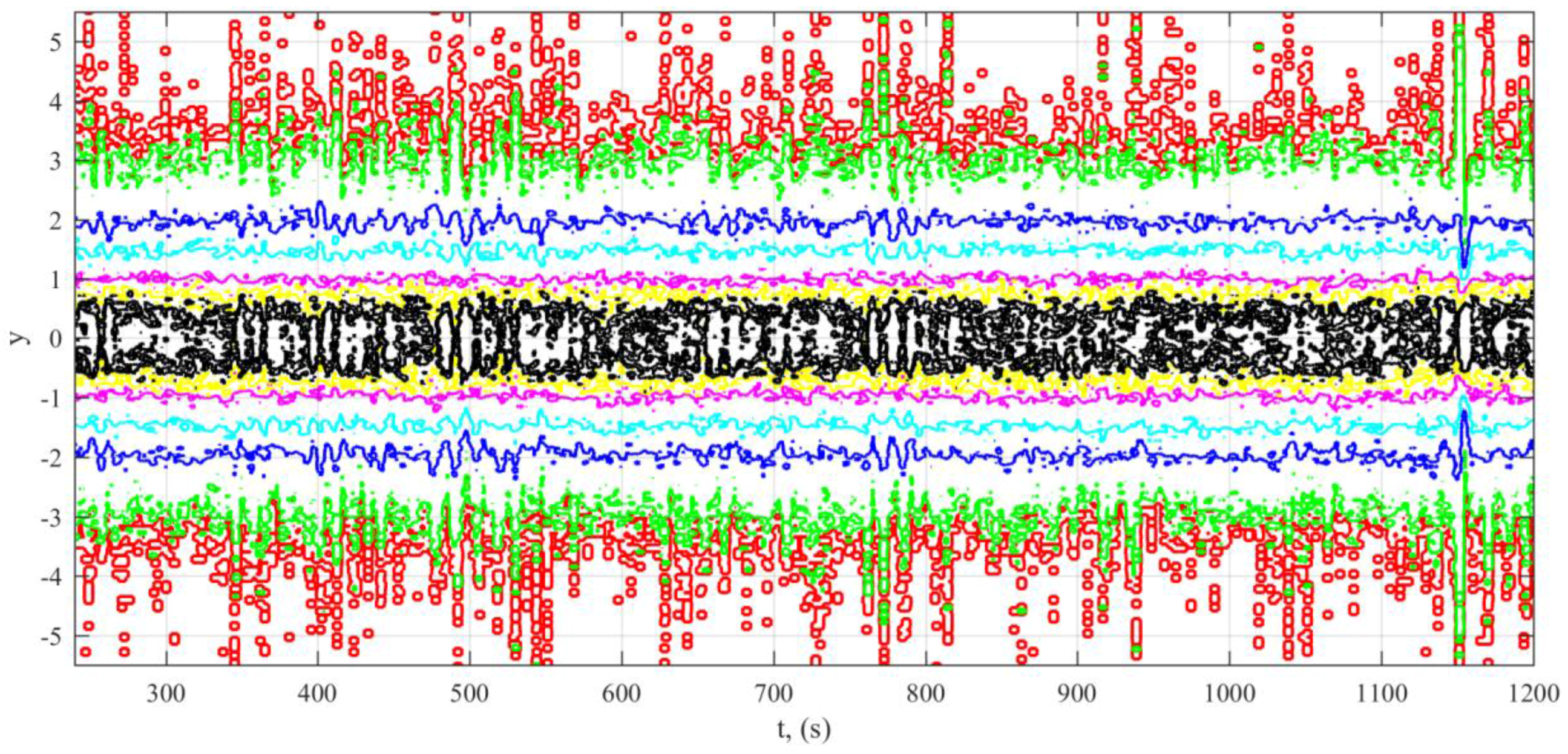
Figure 6 shows the lines of equal probability for the same values w(y) that are seen in Figure 5, yet here the accumulation time T is equal to 1 s. No changes resulting from the passage of the vessel and the motor boat were observed (see Figure 1) with this accumulation time.
The proper T value in order to detect change in PDF is determined in accordance with the set task. If the conditions of applicability of the central limit theorem are met, then with increase of T, the PDF comes close to the Gaussian distribution. The PDF for the nonstationary hydroacoustic noise in the shallow waters with intense shipping traffic may significantly differ from the Gaussian distribution, especially when vessels with distinct propeller cavitation are passing by the receiving system.
Applicable to the tasks of detection of signals of final duration, the practical interest lies is estimation of PDF at the time intervals that correspond to the durations of the expected signals. When using “long” code words or “line-by-line” transmission of images via hydroacoustic communication channel, the proper T value can be anywhere from a fraction of a second to dozens of seconds.
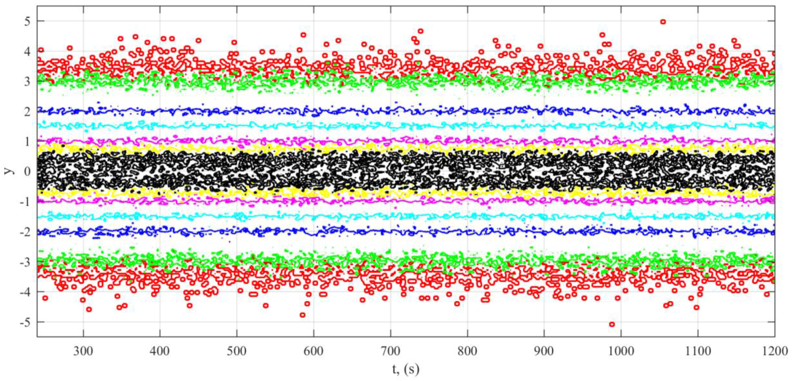
For comparison, Figure 7 and Figure 8 show the lines of equal probability for low-frequency white Gaussian noise at the output of Brüel & Kjær Sine Random Generator Type 1027 (Brüel & Kjær, Naerum, Denmark). The noise was digitalized, filtered, normalized, and processed by the levels—in the same manner as earlier described underwater noise signal with the accumulation time of 10 s and 1 s, respectively.
From comparisons of Figure 5, Figure 6, Figure 7 and Figure 8, it is evident that with the decrease of accumulation time, the differences of the Gaussian distribution increase most notably in both areas of high and low probable sample values; changes in the intermediate area of sample values are less distinct.
4. Conclusions
Taking into consideration the results of the research conducted, the following conclusions can be drawn:
- With accumulation time of 10 s, the most notable differences of the signal at the output of program module that implements AGC from the Gaussian distribution are observed in both areas of high and low probable sample values; differences from the Gaussianity in the intermediate area of sample values are less notable.
- With the decrease of accumulation time, the differences from the Gaussian distribution increase most notably in the areas that correspond to the most probable sample values and the least probable sample values; changes in the intermediate area of probable sample values are less notable.
- The research confirms the possibility of using the stationary noise model at the output of the described AGC system for the studied fragment of hydroacoustic noise, including fragments with propeller cavitations as an initial approach.
Acknowledgments
All sources of funding of the study should be disclosed. Please clearly indicate grants that you have received in support of your research work. Clearly state if you received funds for covering the costs to publish in open access.
Author Contributions
Sergey Gorovoy and Alexey Kiryanov conceived and designed the experiments; Sergey Gorovoy, Alexey Kiryanov and Evgeniy Zheldak performed the experiments, analyzed the data and wrote the paper.
Conflicts of Interest
The authors declare no conflict of interest.
References
- McCarthy, E. International Regulation of Underwater Sound; Kluwer Academic Publisher: New York, NY, USA, 2004. [Google Scholar]
- Robinson, S.P.; Lepper, P.A.; Hazelwood, R.A. Good Practice Guide for Underwater Noise Measurement; NPL Good Practice Guide No. 133; National Measurement Office, Marine Scotland, The Crown Estate: Edinburgh, UK, 2014; ISSN 1368-6550.
- Carey, W.M.; Evans, R.B. Ocean Ambient Noise: Measurement and Theory; Springer: New York, NY, USA, 2011. [Google Scholar]
- De Jong, C.A.F.; Ainslie, M.A.; Blacquière, G. Standard for Measurement and Monitoring of Underwater Noise, Part II: Procedures for Measuring Underwater Noise in Connection with Offshore Wind Farm Licensing; Report TNO-DV 2011 C251; TNO: The Hague, The Netherlands, 2011. [Google Scholar]
- Gorovoy, S.; Kiryanov, A.; Zheldac, E. Characteristic of underwater noise near the west roadstead of the port of Vladivostok. Proc. Meet. Acoust. 2016, 24, 070016. [Google Scholar] [CrossRef]
- Gorovoy, S. Two-dimensional and three-dimensional probability density functions of underwater noise near the port of Vladivostok. Proc. Meet. Acoust. 2015, 24, 070026. [Google Scholar] [CrossRef]
- Buckingham, M.J. Cross-correlation in band-limited ocean ambient noise fields. J. Acoust. Soc. Am. 2012, 132, 2643–2657. [Google Scholar] [CrossRef] [PubMed]
- Katsnelson, B.G.; Petnikov, V.G. Shallow Water Acoustic; Springer: Chichester, UK, 2002; ISBN 1-85233-184-4. [Google Scholar]
- Davenport, W.B. A Study of Speech Probability Distributions; Technical Report No. 148; Institute of Technology, Research Laboratory of Electronics: Cambridge, MA, USA, 1950; Available online: http://hdl.handle.net/1721.1/4905 (accessed on 15 January 2018).
- Bardishev, V.I.; Kozhelupova, N.G.; Krishnii, V.I. Study of underwater noise distribution features in sea and ocean coastal zones. Acoust. Phys. 1973, 19, 129–132. [Google Scholar]
- Scott, D.W. Multivariate Density Estimation: Theory, Practice, and Visualization; John Wiley: New York, NY, USA, 1992. [Google Scholar]
- Härdle, W.K.; Simar, L. Applied Multivariate Statistical Analysis; Springer: New York, NY, USA, 2012; ISBN 978-3-642-17228-1. [Google Scholar]
- Bosq, D. Nonparametric Statistics for Stochastic Processes: Estimation and Prediction; Springer: New York, NY, USA, 1996; ISBN 978-0-387-94713-6. [Google Scholar]
- Cramér, H. Mathematical Methods of Statistics; Princeton University Press: Princeton, NJ, USA, 1946. [Google Scholar]
Figure 1.
Oscillogram (top) and spectrogram (bottom) of the signal at the hydrophone preamplifier output during the passage of a vessel and a boat. Over the spectrogram there is a scale that illustrates the dependence of color on the levels of spectral components of the signal in dB. The scale is conventional.

Figure 2.
Oscillogram (top) and spectrogram (bottom) with a scale reflecting dependence of color on the levels of spectral components of the signal in dB at the output of program module that is implementing automatic gain control (AGC) and normalization of the signal by the level. The scale is conventional.

Figure 3.
Fragment of characteristics of the same signal (Figure 2, top). Top—oscillogram, bottom left—the signal fragment mean spectrum, bottom right—the signal initial fragment of the time correlation function.
Figure 3.
Fragment of characteristics of the same signal (Figure 2, top). Top—oscillogram, bottom left—the signal fragment mean spectrum, bottom right—the signal initial fragment of the time correlation function.

Figure 4.
Underwater noise signal after AGC and normalization by the level. Time dependence of the smoothed histograms for T = 10 s.
Figure 4.
Underwater noise signal after AGC and normalization by the level. Time dependence of the smoothed histograms for T = 10 s.

Figure 5.
Underwater noise signal after AGC and normalization by the level. Lines of equal probability for consecutive probability density function (PDF) for T = 10 s, see Figure 4. This is lines of equal probability of the values of w(y): 0.000134 (red), 0.004432 (green), 0.053991 (blue), 0.1295 (cyan), 0.241971 (magenta), 0.3521 (yellow), 0.3867 (black). For the Gaussian distribution with the mean equal to 0 and variance equal to 1, this would be corresponding to the straight lines—also in accordance with values of y: ±4, ±3, ±2, ±1.5, ±1, ±0.5, ±0.25.

Figure 6.
Underwater noise signal after AGC and normalization by the level. Lines of equal probability for consecutive PDF for T = 1 s. This is lines of equal probability of the values of w(y): 0.000134 (red), 0.004432 (green), 0.053991 (blue), 0.1295 (cyan), 0.241971 (magenta), 0.3521 (yellow), 0.3867 (black). For the Gaussian distribution with the mean equal to 0 and variance equal to 1, this would be corresponding to the straight lines—also in accordance with values of y: ±4, ±3, ±2, ±1.5, ±1, ±0.5, ±0.25.

Figure 7.
White noise after normalization by the level. Lines of equal probability for consecutive PDF for T = 10 s. This is lines of equal probability of the values of w(y): 0.000134 (red), 0.004432 (green), 0.053991 (blue), 0.1295 (cyan), 0.241971 (magenta), 0.3521 (yellow), 0.3867 (black). For the Gaussian distribution with the mean equal to 0 and variance equal to 1, this would be corresponding to the straight lines—also in accordance with values of y: ±4, ±3, ±2, ±1.5, ±1, ±0.5, ±0.25.

Figure 8.
White noise after normalization by the level. Lines of equal probability for consecutive PDF for T = 1 s. This is lines of equal probability of the values of w(y): 0.000134 (red), 0.004432 (green), 0.053991 (blue), 0.1295 (cyan), 0.241971 (magenta), 0.3521 (yellow), 0.3867 (black). For the Gaussian distribution with the mean equal to 0 and variance equal to 1, this would be corresponding to the straight lines—also in accordance with values of y: ±4, ±3, ±2, ±1.5, ±1, ±0.5, ±0.25.

© 2018 by the authors. Licensee MDPI, Basel, Switzerland. This article is an open access article distributed under the terms and conditions of the Creative Commons Attribution (CC BY) license (http://creativecommons.org/licenses/by/4.0/).
Share and Cite
MDPI and ACS Style
Gorovoy, S.; Kiryanov, A.; Zheldak, E. Variability of Hydroacoustic Noise Probability Density Function at the Output of Automatic Gain Control System. Appl. Sci. 2018, 8, 142. https://doi.org/10.3390/app8010142
AMA Style
Gorovoy S, Kiryanov A, Zheldak E. Variability of Hydroacoustic Noise Probability Density Function at the Output of Automatic Gain Control System. Applied Sciences. 2018; 8(1):142. https://doi.org/10.3390/app8010142
Chicago/Turabian StyleGorovoy, Sergey, Alexey Kiryanov, and Evgeniy Zheldak. 2018. "Variability of Hydroacoustic Noise Probability Density Function at the Output of Automatic Gain Control System" Applied Sciences 8, no. 1: 142. https://doi.org/10.3390/app8010142
Note that from the first issue of 2016, this journal uses article numbers instead of page numbers. See further details here.