Underwater Cylindrical Object Detection Using the Spectral Features of Active Sonar Signals with Logistic Regression Models


1
School of Electronic Engineering, Soongsil University, Seoul 06978, Korea
2
Applied Physics Laboratory, University of Washington, 1013 NE 40th St, Seattle, WA 98105, USA
3
Agency of Defences and Developments, Jinhae 51678, Korea
*
Author to whom correspondence should be addressed.
†
These authors contributed equally to this work.
Appl. Sci. 2018, 8(1), 116; https://doi.org/10.3390/app8010116
Submission received: 24 October 2017
/
Revised: 8 January 2018
/
Accepted: 14 January 2018
/
Published: 15 January 2018
(This article belongs to the Special Issue Underwater Acoustics, Communications and Information Processing)
Abstract
:The issue of detecting objects bottoming on the sea floor is significant in various fields including civilian and military areas. The objective of this study is to investigate the logistic regression model to discriminate the target from the clutter and to verify the possibility of applying the model trained by the simulated data generated by the mathematical model to the real experimental data because it is not easy to obtain sufficient data in the underwater field. In the first stage of this study, when the clutter signal energy is so strong that the detection of a target is difficult, the logistic regression model is employed to distinguish the strong clutter signal and the target signal. Previous studies have found that if the clutter energy is larger, false detection occurs even for the various existing detection schemes. For this reason, the discrete Fourier transform (DFT) magnitude spectrum of acoustic signals received by active sonar is applied to train the model to distinguish whether the received signal contains a target signal or not. The goodness of fit of the model is verified in terms of receiver operation characteristic (ROC), area under ROC curve (AUC), and classification table. The detection performance of the proposed model is evaluated in terms of detection rate according to target to clutter ratio (TCR). Furthermore, the real experimental data are employed to test the proposed approach. When using the experimental data to test the model, the logistic regression model is trained by the simulated data that are generated based on the mathematical model for the backscattering of the cylindrical object. The mathematical model is developed according to the size of the cylinder used in the experiment. Since the information on the experimental environment including the sound speed, the sediment type and such is not available, once simulated data are generated under various conditions, valid simulated data are selected using 70% of the experiment cylinder data. The selected simulated data are used to train the model. Randomly selected experiment cylinder data, which are 70% of the total experimental cylinder data, and the rock measurement data are used to test the model. This process is repeatedly carried out 1000 times. The results show that the proposed method is effective under the circumstance where experimental data are not sufficient and a mathematical model is available for a target.
1. Introduction
Detection of objects in the unfavorable environment is an important issue that receives great interest in various fields, including the military and civilian areas. Detecting an object on a seafloor composed of sand and mud in the shallow water is a significant technology in the military detection field [1,2,3]. In this problem, the reflections coming from the clutter surrounding a target and the ambient noise are the main hurdles. Furthermore, when the target is lying on the seabed in the shallow water, the detection is more difficult because the noise radiated by the target is maintained to be minimal and its target strength is relatively reduced by a narrow incident angle of the signal from the active sonar source. Thus, effective detection methods under such an environment are required to be developed.
The actual underwater environment considered in this study is the Yellow Sea in Korea. The depth of the Yellow Sea is less than 100 m, so it may be anticipated that small submarines can find places on the sea floor to exploit. Thus, the target considered here is like a cylinder with a length of 20 m and a radius of 2 m. For detecting this type of target at a distance from 500 to 800 m, an active sonar is designed with the linearly frequency modulated (LFM) signal of a band from 6 kHz to 20 kHz and a planar array of 9 m by 11 m [3,4,5], which has a bearing-range resolution of 0.67 . Figure 1 schematically illustrates the underwater environment considered in this study. Since the detection area is from 500 m to 800 m, the grazing angle decreases from 10.2 to 6.4, which can hardly be distinguished by the sonar system due to a relatively wide vertical beam width. Since this sonar system uses a mid-frequency LFM signal, imaging is impossible and the detection method is based on the approach proposed in [3,6].
There are several approaches to the similar problem. One of them is the application of a side scan sonar to acquire images of the detection fields [7,8,9]. Unfortunately, obtaining clean images by a side scan sonar requires slow scan speed and additional efforts are required to recognize a target submerged into the sediments. Various studies have been carried out from the viewpoint of classification. In [10], Fawcett et al. investigated four information fusion methods for classification of underwater objects through two sidescan sonar images. Huang et al. used various machine learning models to create prediction maps and prediction uncertainty maps [11]. The study presented in [12] proposed an automated target detection approach that combines image based feature extraction, independent component analysis, and unsupervised classification. It is demonstrated its suitability for detecting small targets in side scan sonar imagery. In [13], Williams and Fakiris introduced a new context-dependent classification algorithm and demonstrated its performance using measured data. In this situation, the approach employed by the Applied Physics Lab. (APL) at the University of Washington, Seattle, WA, USA draws attention for detecting sea mines at the bottom of the seabed in the shallow sea [1,2]. This approach is based on the mathematical target and seabed models to obtain the features of the bottoming target, which are simultaneously verified with the measurements. Through this study, the target signature database is constructed to enable the detection probability of the active sonar system to increase. However, this approach has a disadvantage of investigating whether each received signal matches any component in the database. This is very time-consuming. Thus, in order to save this time and effort, the signal energy-based threshold scheme can be applied. That is, for a specific received signal that has greater energy than the prespecified threshold only, comparison with the database is carried out, but this still needs comparison time.
The logistic regression is one of the supervised learning models for classification, which trains a set of parameters that maximizes the likelihood of the categories for training data [14]. Williams et al. [15] employed the infinitely imbalanced logistic regression [16] to the problem of mine classification on ground-penetrating radar images and sidescan sonar images exploiting the imbalanced characteristic of information. In [17], the detection of mines or other objects on the seabed from multiple side-scan sonar views is considered and the logistic regression models are used for comparison. In [18], the semi-supervised and active learning schemes are developed and applied to detection of buried unexploded ordnances (UXO’s) using several machine learning models including the logistic regression. Note that the previous works are based on target images while the approach in this study relies on the matched filtered signal samples.
In this paper, the logistic regression model is employed for this detection problem since the target detection is a kind of classification problem. As mentioned above, the energy of the received signal is one of the various features. The reflected signals from the hard sediment such as rocks can trigger a false alarm by the active sonar system, which degrades the system performance. In order to improve detection performance and speed, the logistic regression model is trained by the feature vectors of the target in the clutter and those of the clutter without any target. For generating the target signals in the clutter, the target response with respect to the linearly frequency modulated signal is developed by the cylindrical object model proposed by Ye [19] and the clutter signals are generated based on the K-distribution model introduced by Abraham and Lyons [3,20]. The interaction between the target and the contacted sediment and the resulting multipath components are developed using the similar approach presented in [2].
The objective of this study is to investigate whether the logistic regression model trained through simulated data generated by the mathematical model for a cylinder’s backscattering can operate for the experimental data. The motivation of this study is that, in general, it is not easy to obtain abundant experimental data in the underwater field. Thus, it is difficult to train the model with sufficient amount of the data. For this reason, the simulated data are generated by using the mathematical model of a cylinder, and then applied to the logistic regression model to perform cross-validation of the model. In the following step, the logistic regression models trained using the simulated data based on the mathematical model are evaluated using the experimental data. In the first stage, the feature vector consists of the magnitude spectrum of the signal, that is, the absolute value of the discrete Fourier transform (DFT) of the signal because the target response has different spectrum shape from that of the clutter signal, which is random with the K-distribution. In addition, the magnitude spectrum is dependent on the rotation angle of the target. These facts have been reflected in the generation of the feature vectors. The training method employed in this work is a kind of the truncated Newton approach for maximum likelihood estimation [21]. For the cross validation, the shuffle and split is employed. The performance of the model is evaluated in terms of the receiver operation characteristic (ROC) curve and its area under ROC curve (AUC), and the classification table. Since the information on the environment including the sound speed, the sediment type, and so on is not available with the data, the simulated data are generated under various conditions when applying the model to the experimental data, and the valid data are selected using the samples of the experimental data and the selected simulated data are used to train the logistic regression model and the samples randomly selected experimental data are applied to evaluate the model.
The paper is organized as follows. Section 2 briefly introduces the logistic regression model and its features. In Section 3, the underwater environment considered in this study is described and the target scattering and clutter signal models are introduced. The generation of the feature vector is explained in Section 4. In Section 5, the performance of the logistic regression model with the simulated data is presented and discussed. Section 6 demonstrates the performance of the proposed approach with the experimental data. Finally, the paper is concluded in Section 7.
2. Introduction to Logistic Regression
Logistic regression is a statistical model that expresses its input–output relationship stochastically through the logistic function, where the output of the logistic regression model is categorical. It is characterized by high analytical power and adaptability in determining the relationship between two or more variables. This method has already been applied in many research fields because of its high performance in a binary classification problem [14].
In this study, the vector consisting of d feature values represents the i-th feature vector while the scalar represents its corresponding category label (e.g., clutter or target). The binary logistic regression model considered in this study has the learning parameters vector and scalar . For a set of N labeled data points , the cost function for the parameters and b is the log-likelihood of the defined by
where represents the probability that the output belongs to the category of 1 given and N is the number of the feature vectors. For the binary logistic model considered here, the probability is given by
where the superscript T represents transpose.
In order to find the optimal learning parameters and b that maximize the likelihood function for a given training set, the trust region Newton scheme [21] is employed in this study. This scheme relies on approximate Newton stages in the initial stage but obtains fast convergence. The performance of the model is evaluated by measuring the AUC of the ROC curves [22], the classification tables for the test data set and the detection rate according to the target-to-clutter ratio (TCR), which is defined by
where and are the power spectral densities of the target signal and the seabed clutter at frequency bin , respectively, and Q is the total number of frequency bins in the section of the signal bandwidth.
3. Simulated Underwater Environment
In this study, detection of a cylinder lying on the seabed is considered. This is an important issue that can be extended to the detection of undersea mines or submarines. The situation considered in this study are well described in [2,3,4,5], which schematically is displayed in Figure 1. In the conventional methods, the target detection is made by comparing the matched filtered signal with the prespecified threshold. This scheme can cause false alarms when the number of clutters in the vicinity increases or when the hard sediments are located in the detection area. For improving the detection performance, a logistic regression is utilized to discriminate the case of target present from the case of no target using the spectral components. In order to train the logistic regression, the target scattering signal and the clutter signal is required. If real measurements are available and sufficient, using the measurements is most effective for training. Otherwise, the data should be generated by the models that describe the real situation. In the following, the models for the target and clutter signals are briefly presented.
3.1. Scattering and Path Models for Target
For generating the target scattering signal, the scattering model of a cylindrical object proposed by Ye [2,19] is employed in this study. This is developed by applying Kirchhoff’s scalar scattering theory to the problem of finite cylinders. The model describes the body and end scatterings of the object separately by dividing the surface area of the object into the cylindrical body and the flat end, respectively. In this study, the reverberation of a cylinder of enclosed finite length is induced by combining scattering of a body part and scattering from its ends [2,23,24].
Assuming that the transmission speed of sound is constant and the distance between source and target is enough, the path model that is coming back from the source to the receiver via the target relies on the simplified model proposed in [2,23,25].
The diameter and length of the cylinder considered in the simulation are assumed to be 2 m wide and 20 m. The area observed by the sonar system is limited to a range of 500 m to 800 m from the sonar transceiver in terms of bottom straight distance. The sound velocity is assumed to be 1500 m/s, and the sampling frequency is set to 40 kHz. The transmitted signal is a linearly frequency modulated (LFM) signal with a center frequency of 13 kHz and a bandwidth of 14 kHz. The sonar system performs matched filtering on the received signal [26]. In the stage of matched filtering, the receiver convolves the received signals with the time reversed version of the transmitted LFM signal, which gives pulse-compressed signals. In this study, the match filtered signals are applied to generating the feature vectors for the logistic regression model.
3.2. Reverberation Models for Seabed
In this study, it is assumed that the patches where scattering occurs are evenly distributed on the seabed. Thus, a model for the scattering of patches within a resolution cell range is required. The resolution cell of sonar in general form and a model for the patches are illustrated in Figure 2.
The Rayleigh distribution is applied using the central limit theorem, in which the sum of sufficient random distributions converges to a Gaussian distribution under the assumption that sufficiently many scatterers are distributed in the resolution cell. However, for active sonar systems with high resolution that have recently become available owing to the current development of technology, the number of reverberation components that influence the given resolution cell could be reduced. Therefore, the central limit theorem cannot be applied and a non-Rayleigh distribution is applied. As shown in Figure 1, a shallow water environment with a depth of 100 m is assumed and the LFM signal with a band from 6 kHz to 20 kHz is used for the transmit signal of active sonar. Because the swarth size is not large on the seabed, a non-Rayleigh distribution can be applied considering a finite number of scatterers. Abraham and Lyons derived reverberation signals by applying the K-distribution instead of the Rayleigh distribution under this assumption [20]. The distribution of the envelope of a matched filtered signal, which is received from a finite number of scatterers, becomes the K-distribution. The shape parameter of the K-distribution is related to the number of scatterers while the scale parameter is determined by the mean size of the scatterers [27]. The K-distribution is convenient in various environments and situations according to the shape parameters and scale parameters. In this study, the shape parameter is set to 1 and the scale parameter is set to 1. Then, the clutter signal power becomes 1 since the multiplication between the shape and scale parameters is the expectation of clutter power. For a given TCR, the clutter signal is scaled with respect to the target signal power [28]. Note that for the shape parameter greater than 50, the distribution converges to the Rayleigh distribution.
4. Feature Vector Generation
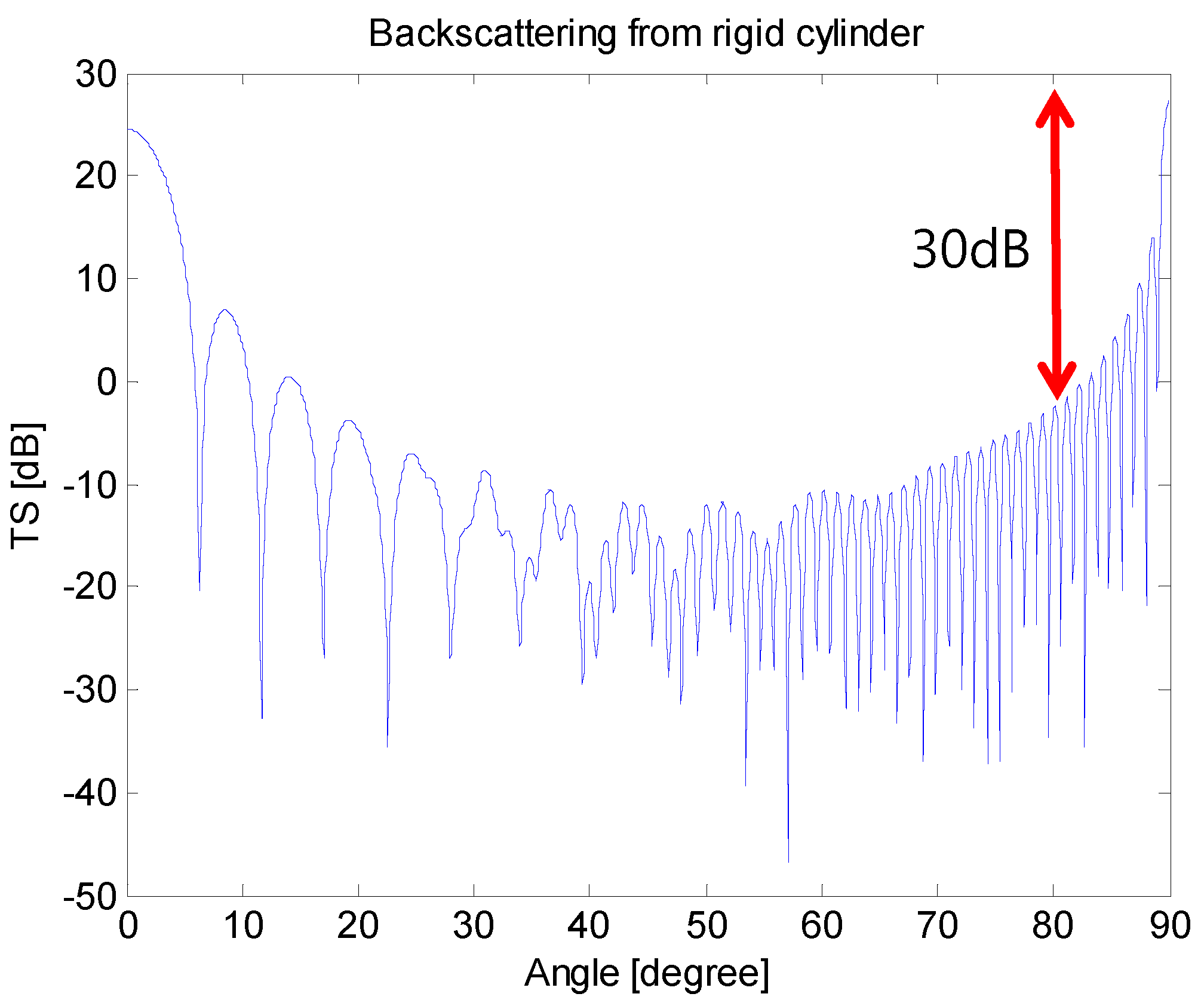
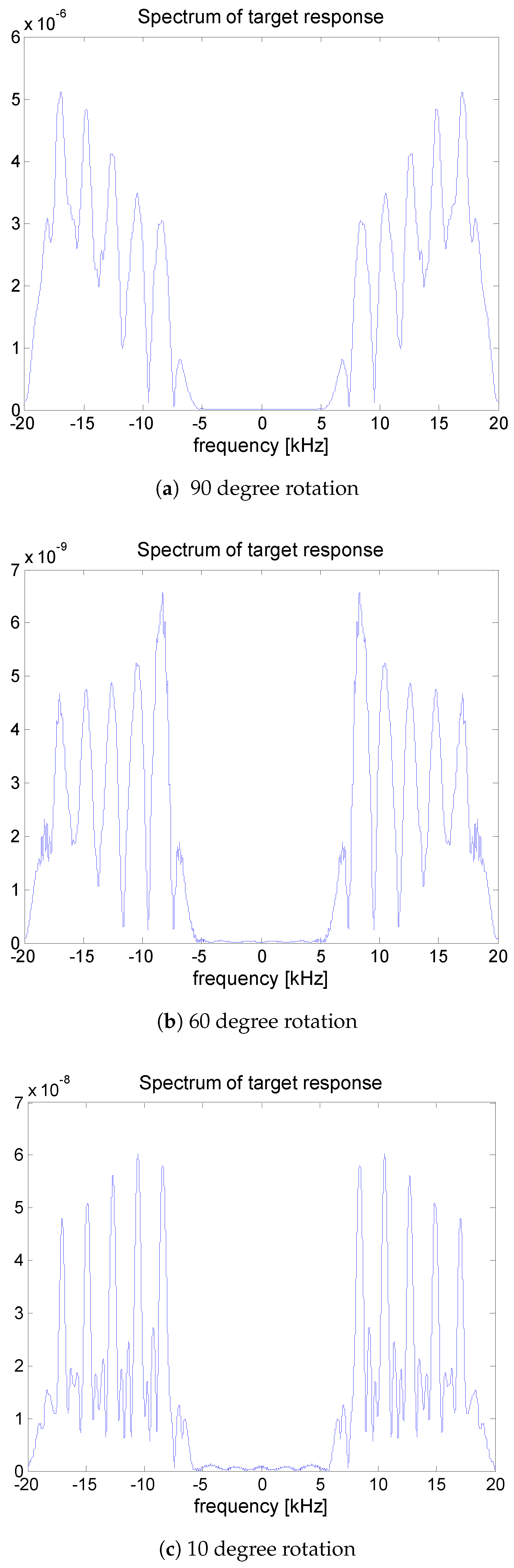
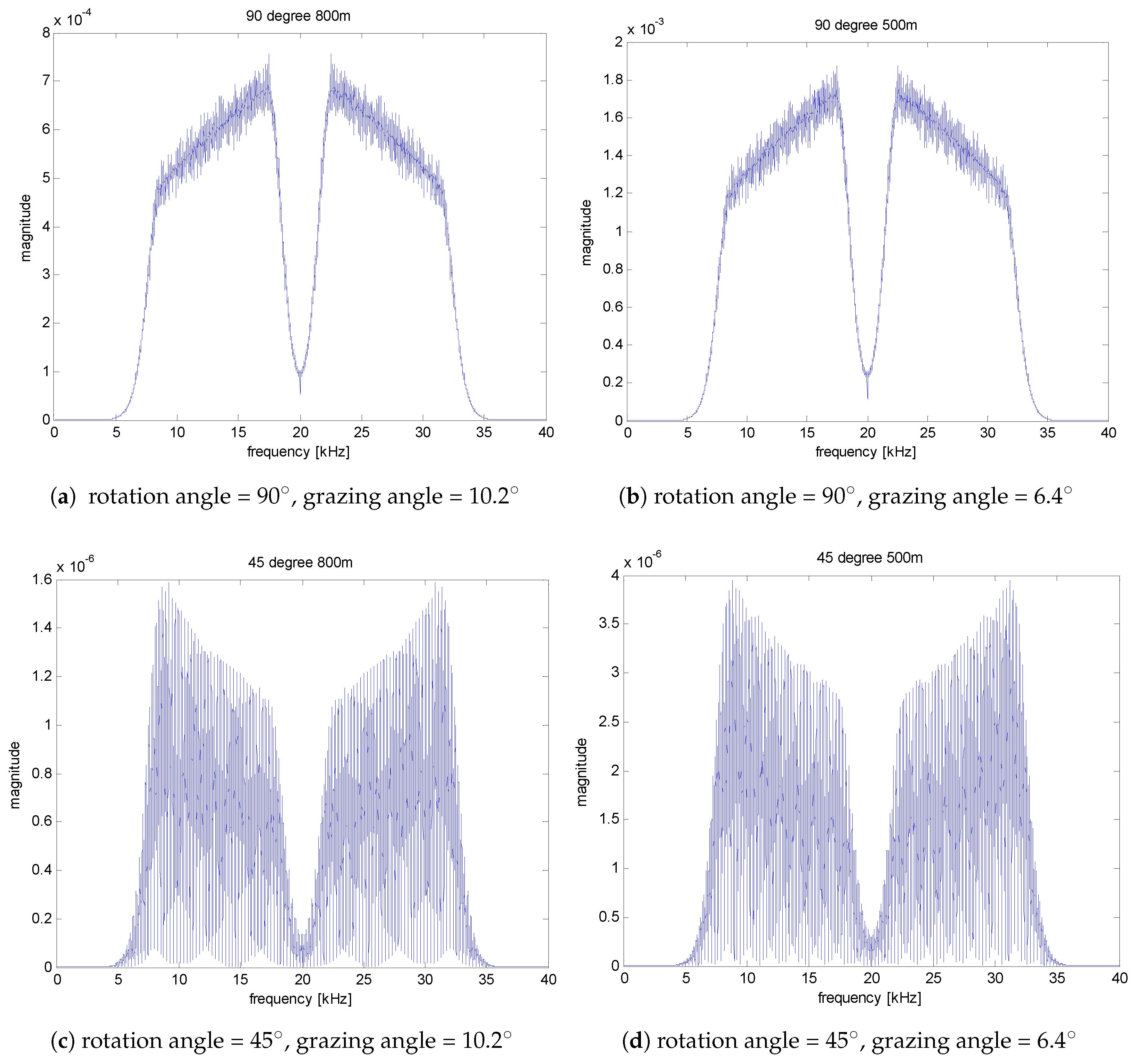
For generating a feature vector for the logistic regression model, the DFT is applied to the matched filtering output of the sonar, the magnitude of this DFT result is used as a feature. The target strength is shown in Figure 3 according to the rotation angle of the target with respect to the incident signal. A significant change in target strength can be observed depending on the angle. Figure 4 shows examples of the magnitude spectrum for the received signal for rotation angles of 10 degrees, 60 degrees, and 90 degrees, respectively. It is observed that the spectrum varies depending on the angle. The feature vector reflecting these spectral characteristics are utilized in the logistic regression model. Note that the target response is depending on the grazing angle from the sonar. However, since the water depth is 100 m and the target is located in the range from 500 m to 800 m in this study, the grazing angle varies from 10.2 to 6.4, which does not make a notable difference in the spectrum, as observed in Figure 5.
The data set employed to develop the model can be denoted by , which consists of the feature vector composed of the magnitude of the DFT of the received signal and the corresponding class label , which indicates the existence of the target. That is, the label represents the state that there is a target signal in the feature vector while the label indicates no target.
In this study, 22,000 feature vectors are generated; 11,000 feature vectors are obtained from the signals representing that a target is in the detection range while the remaining 11,000 vectors are from the clutter signals without a target in the region.
For the case that a target is present, the rotation angle of the target is changed by 10 degrees from 0 degrees to 90 degrees. For each rotation angle, TCR is increased by 1 dB from −5 dB to 5 dB. 100 signals, , are generated for each TCR and each rotation angle, where is the target response and is the clutter signal.
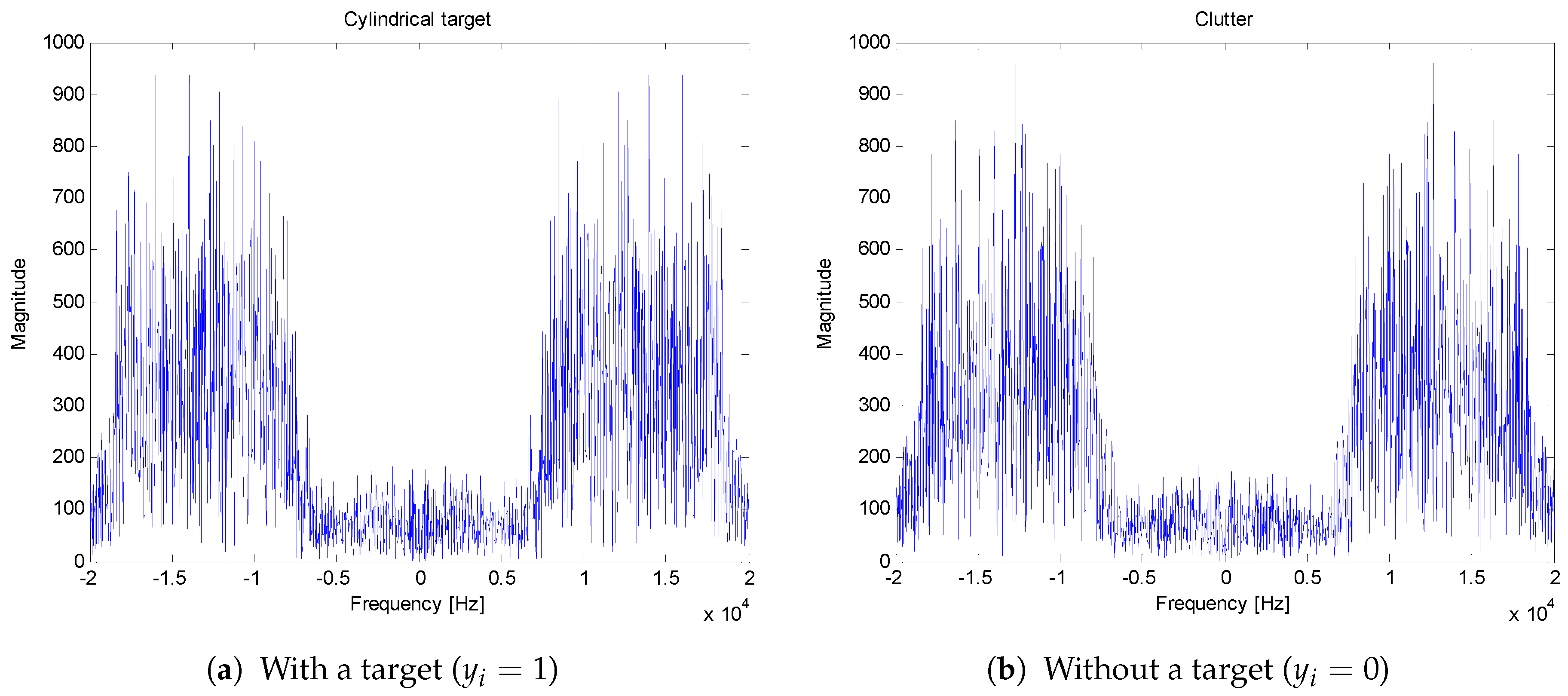
Whenever one feature vector with is generated, the same condition is applied to the generation of the corresponding clutter signal and another clutter signal with the same power of the target signal for a given TCR is generated and added to the clutter signal . Note that each signal consists of 1501 samples and DFT is performed to obtain a magnitude of each frequency band to construct a feature vector. Figure 6 shows an example of the time domain waveform pair with (Figure 6a) and (Figure 6b). The two waveforms are very similar and the magnitude spectra of the two waveforms shown in Figure 6 are shown in Figure 7. It is difficult to discriminate one from another. However, the magnitude spectrum in Figure 7a has a specific spectrum structure as shown in Figure 4.
Note that the magnitude spectrum is an even function for a real signal. Since the feature vector is generated from the magnitude spectrum of the DFT of the signal, the size of the feature vector is half of the length of the DFT, which can reduce the number of learning parameters. Since the advantage of using the magnitude spectrum is that delay or time synchronization is not critical, the energy of the signal of interest should be just in the DFT window interval.
5. Learning and Prediction
In order to find the learning parameter and b in the logistic regression model (2), the trust region Newton method [21] is employed in the learning stage using the liblinear library [29]. The validation of the learned model is carried out in two ways. The first approach for the cross validation is the shuffle and split cross validation. Eighty percent of the total data set is randomly selected for learning and the remaining is used for prediction. This cross-validation is carried out 10 times for evaluating the average performance. The second one is to divide the total data set into two groups. In this case, 50% of the data is randomly selected for each TCR and each rotation angle to evaluate the detection performance of the model for each TCR.
The goodness-of-fit of the learned model is assessed using the classification table [30,31] and the AUC [22,31]. The ROC curve shows the performance of the model in two dimensions. Therefore, intuitive judgment is difficult in comparing or evaluating performance. Considering this aspect, it is necessary to show performance as a single scalar value. The AUC value is between 0 and 1 because it represents the area of the unit square in which the ROC curve is drawn and computation of AUC is easy. It is known that AUC = 0.5 represents no discrimination, 0.8 ≤ AUC < 0.9 is evaluated as excellent discrimination, and AUC is considered outstanding discrimination [14]. As another performance index, the classification table is a useful table for visualizing the performance of algorithms in statistical classification problems.
5.1. 8:2 Shuffle-Split Cross-Validation
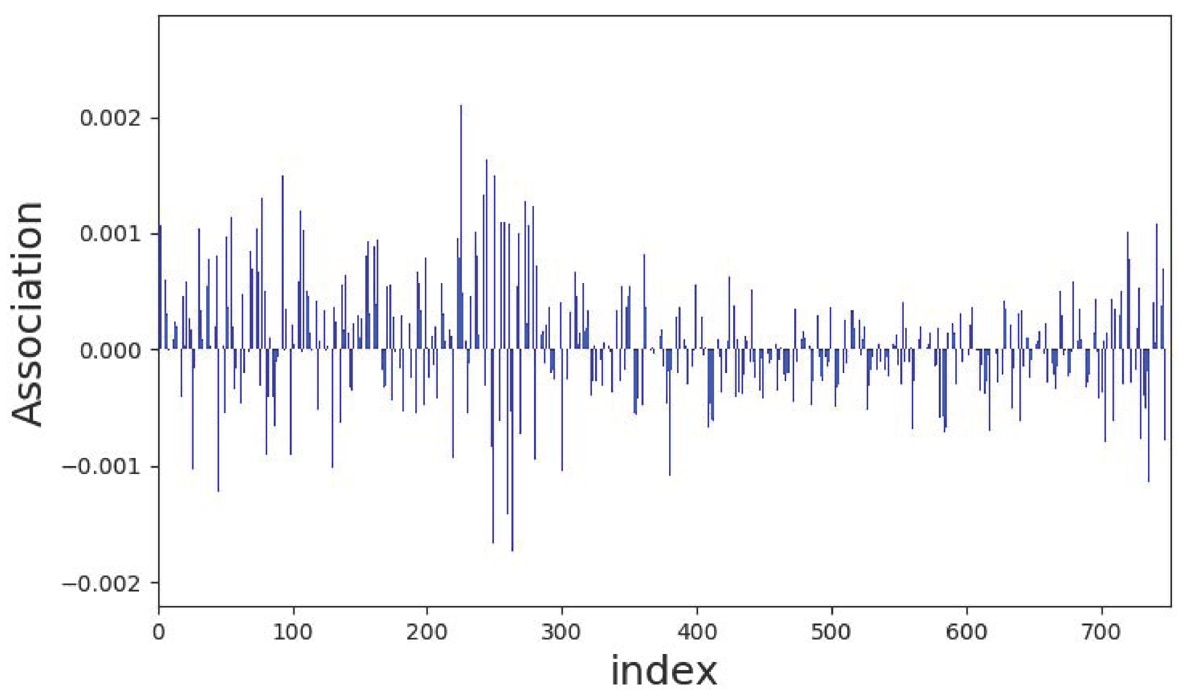
In this experiment, the training and test data are randomly selected at 8:2 for the 22,000 data and training and testing are performed ten times. Figure 8 shows one example of the learning parameters obtained through ten training sessions. It is observed in the figure that the parameters marked indices 50 to 300 have relatively larger magnitudes. These parameters are closely related to the significant spectral components of the target signals. Figure 9 shows one example of the ROC curves for the ten trials. The mean of ten AUC values is 0.8983 and the standard deviation is 0.0036. As mentioned previously, the model can be assessed as an excellent model. In Table 1, the accumulated classification table is demonstrated for the test data. According to this table, the hit rate of the model is 0.8267.
5.2. Detection Performance
In order to evaluate the detection performance according to TCR, 11,000 training data are selected as mentioned above and the test is performed for each TCR. The AUC and probability of detection are observed for each TCR while the ROC curve is measured for the total test data. Figure 10 shows the learning parameter of the model for the 11,000 training data. The parameters of Figure 10 show a similar shape as in Figure 8.
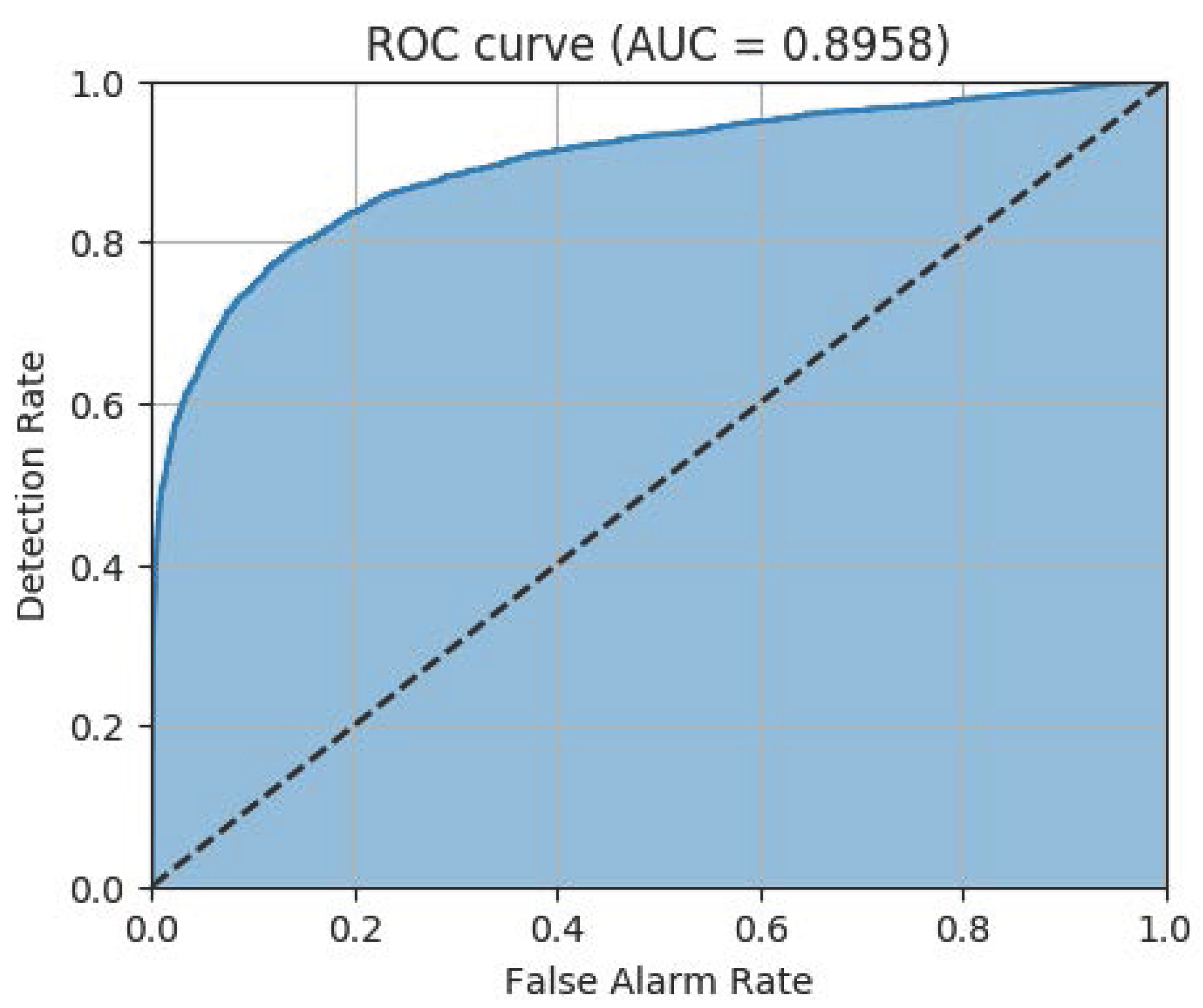
For the 11,000 test data, the ROC curve of the model with the parameters in Figure 10 is displayed in Figure 11. AUC of 0.8958 implies that the model operates as an excellent classifier noting that the worst AUC is 0.5 in binary classification [14]. These results are observed in the classification table of Table 2. According to this table, the hit rate is 0.8115.
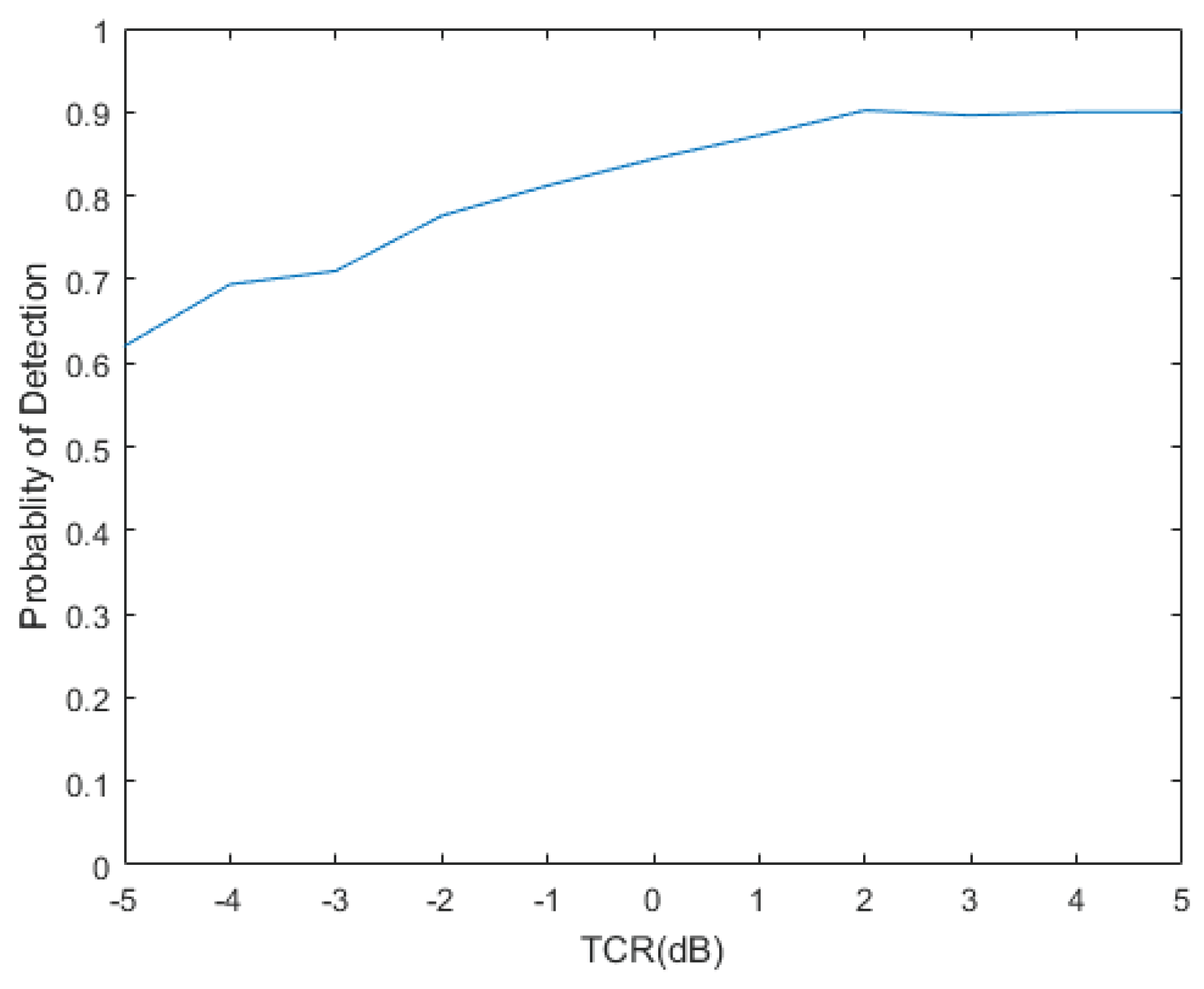
In addition, AUC values according to TCR are displayed in Figure 12. The minimum is 0.74 at TCR = −5 dB while the maximum is 0.94 at TCR = 3 dB. As the target signal power is getting better over the clutter power, AUC improves, which shows excellent discrimination. The probability of detection is plotted with respect to TCR in Figure 13, where the detection probability of 0.62 at TCR of −5 dB is observed, while, for TCR greater than or equal to 2 dB, the detection probability of about 0.9 is maintained.
6. Application to Experimental Data
In this section, the proposed approach is verified through application to real data. The experimental data set used in this application is Pond Experiment 2010 (PondEx10), which was carried out by the Applied Physics Laboratory in the University of Washington (APL-UW), Seattle, WA, USA for identifying and understanding target and environmental factors affecting sonar performance and identifying robust signal characteristics unique to a given underwater unexploded ordnance (UXO) [25,32]. In this application, first, the logistic regression model is trained using the simulated data presented by the method mentioned in Section 3, and the experimental measurements are used to test the trained model. Since the data set considered in this study consists of the backscattering measurements for an aluminum cylinder of 61 cm in length and 30.5 cm in diameter, the simulated data are generated according to this size. The performance is measured in terms of the Receiver Operating Characteristic (ROC) curve and the confusion matrix.
6.1. Experimental Data
The original data sets consist of calibrated cross range and time scattering data from various simple shapes and UXO targets at nine different orientations. The frequency range of the data is 1–30 kHz and the sampling rate is 100 kHz. An understanding of the apparatus that acquired the data can be found in [25]. Among the data sets, the three measurement sets of an aluminum cylinder and two rocks (Rock 1 and Rock 2) are utilized for this investigation. The objects were located 10 m horizontally from the rail-mounted active sonar system and are proud on the sand sediment. Note that the sonar system uses a 6 ms linear frequency modulated (LFM) transmit signal. Each set consists of nine measurement groups according to object orientations from degree to 80 degree with 20 degree increment noting that 0 degrees is broadside in the experiment. Each group has 1600 time series of 2000 samples. Figure 14 displays 2D plots of the time series of the objects at the orientation of 0 degrees.
In this evaluation, two measurement groups are constituted by selecting 2520 time series randomly from the 3600 cylinder measurements that are located in the cross range from −2.5 to 2.5 m as marked in Figure 14a.The first group is utilized for training the logistic regression model that is used to select the simulated time series while the second group is utilized for testing the model that is trained by the simulated data. In addition, 3600 measurements of Rock 2 are used to test the model while 3600 measurements of Rock 1 are employed to train the model since the clutter model cannot be built due to lack of information on the experiment environment.
A 2000-point DFT is applied to each measurement to obtain its magnitude spectrum. Considering the magnitude spectrum symmetry and the energy distribution, the spectral components between the 100th bin (5 kHz) and the 500th bin (27.5 kHz) are selected to make the 451-component feature vectors.
6.2. Simulated Training Data
The simulated data for training the logistic regression model are generated by using the approach presented above. The four path models [2,23] are made according to the size of aluminum cylinder used in the experiment. Unfortunately, the accurate information on the type and property of sediment in the experiment are not provided, and thus the reflection coefficients of the multi-paths are not known. For this reason, when generating simulated signals, 31 possible combinations of the coefficients are considered, which are listed in Table 3. The rotation angle varies from 0 degrees to 90 degrees with 0.1 degree increment. Thus, the total number of the simulated data is 29,700. Since the simulated data are made without the exact information on the experiment environment, there may be simulated signals that are not correlated to the experimental data. In order to remove such data, the logistic regression model is trained with the experimental data consisting of the aluminum cylinder and Rock 1 measurements, in which the principal component analysis (PCA) [33] is applied to reduce 451 components to 52 components with explained variance of 0.99. This trained model is applied to the simulated data to select feature vectors, which are applied to train the model for the experimental data. In this selection procedure, the average number of the simulated data selected for training data as the cylinder is 21,098 for 1000 trials. The remaining simulated data are used as clutter signals since these simulated data are classified as clutter, which implies that these are more similar to the rock measurement. Note that the measurements of Rock 2 are also used for the clutter signals when testing the model.
6.3. Results
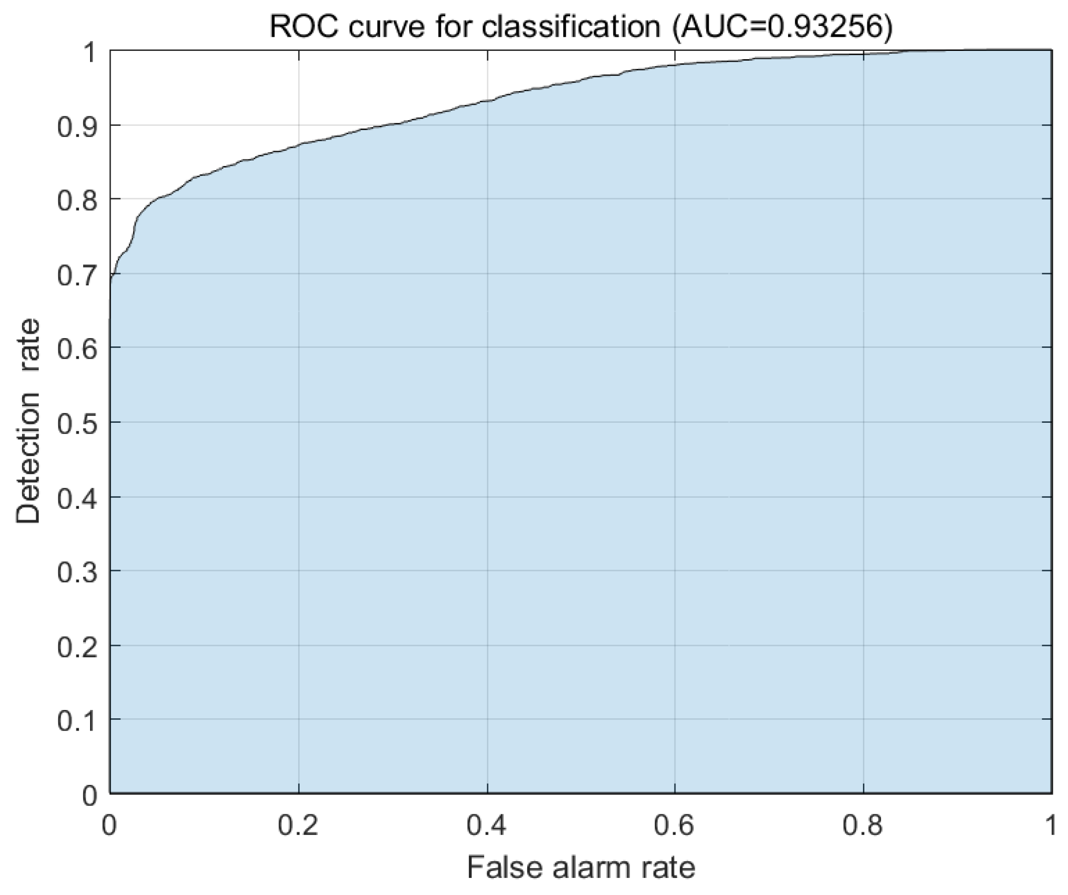
As mentioned above, for 1000 simulations, the simulated data that are classified as target signals are utilized as target feature vectors while the remaining simulated data and the Rock 2 measurements are done as clutter feature vectors. Before training the logistic regression model, PCA is applied to the training vectors to obtain 31 principal components with explained variance of 0.99. In the simulations, the test data consists of 2520 cylinder feature vectors and 3600 feature vectors of the Rock 2 measurements. For 1000 simulations, the mean of AUCs is 0.9325 with its standard deviation of 0.0038. One of the 1000 ROC curves is shown in Figure 15. As mentioned above, the AUC of 0.9325 indicates that the model achieves outstanding discrimination performance [14].
The classification table for the test data, which are averaged over 1000 simulations, is shown in Table 4, where the numbers in parentheses indicate the standard deviation. According to the classification table in Table 4, the average detection rate is 0.7743 with its standard deviation of 0.0115, while the average false alarm rate is 0.058 with its standard deviation of 0.0091.
7. Conclusions
In this paper, it was investigated whether clutters having similar power to the target power can be distinguished by using the logistic regression model. Therefore, the clutter signals considered in this study have such significant power as to lead to a false alarm with the threshold detection scheme. The target signals corresponding to the clutter signals are generated for various rotation angles and for assorted values of TCR. These signals are used to construct the feature vectors and the shuffle–split cross validation technique is applied to the trained model. The models are evaluated in terms of receiver operation characteristic, area under ROC curve, classification table and detection rate. According to the evaluation results, the use of the logistic regression model is very useful for underwater target discrimination. Furthermore, the experimental data are employed to verify the proposed approach. Note that the experimental data are collected for the purpose that is not related to this study. According to the application result, the model trained by the simulated data can discriminate the cylinder from the rock even though it is not perfect. In addition, note that the mathematical model can describe the scattering of the real cylinder well.
In the simulation study, training and testing have been performed using every component of the magnitude spectrum of the received signal. Considering the spectral characteristics of the target and clutter, only the frequency bins carrying the main energy portion can be selected as feature components, which accelerates the processing time by reducing the size of the model. In the simulation study, various TCR conditions were considered since the spectrum is sensitive to magnitude. For further study, the cepstrum may be a good candidate for the feature vector component due to its scale invariance property. The application of the real experiment data reveals the need for the research on the reflection of the multipath components and modeling environments where a target is placed.
Acknowledgments
The authors gratefully acknowledge the financial support provided by Defense Acquisition Program Administration and Agency for Defense Development under the contract (UD140004DD). The authors thank the Applied Physics Laboratory at the University of Washington for providing the experimental data.
Author Contributions
Sungbin Im conceived and designed the experiments; Yoojeong Seo performed the experiments related to the logistic regression model; Baeksan on performed the target signal and the clutter signal modeling; Iksu Seo provided the discussion on the target detection problem in the shallow water; Taebo Shim provided the description on the target signal and the multipath component generation; and Sungbin Im wrote the paper.
Conflicts of Interest
The authors declare no conflict of interest.
References
- Zampolli, M.; Espana, A.L.; Williams, K.L.; Kargl, S.G.; Thorsos, E.I.; Lopes, J.L.; Kennedy, J.L.; Marston, P.L. Low-to mid-frequency scattering from elastic objects on a sand sea floor: Simulation of frequency and aspect dependent structural echoes. J. Comput. Acoust. 2012, 20, 1240007. [Google Scholar] [CrossRef]
- Kargl, S.G.; Shim, T.; Williams, K.L.; Im, S. Scattering from a finite cylindrical target in a waveguide. In OCEANS 2016 MTS/IEEE Monterey; IEEE: Piscataway, NJ, USA, 2016; pp. 1–5. [Google Scholar]
- On, B.; Kim, S.; Moon, W.; Im, S.; Seo, I. Detection of an Object Bottoming at Seabed by the Reflected Signal Modeling. J. Inst. Electron. Inf. Eng. 2016, 53, 55–65. [Google Scholar] [CrossRef]
- Kim, S.; Jung, J.; On, B.; Im, S.; Seo, I. Optimum Frequency Analysis for Sonar Transmit Signal Design. J. Inst. Electron. Inf. Eng. 2016, 53, 47–54. [Google Scholar] [CrossRef]
- Kim, S.; Jung, J.; On, B.; Im, S.; Seo, I. Design of SONAR Array for Detection of Bottoming Cylindrical Objects. J. Inst. Electron. Inf. Eng. 2017, 54, 15–21. [Google Scholar]
- Kim, S.; Im, S.; Shim, T.; Kargl, S.G. Detection of an object bottoming at seabed through modeling consecutive reflected signals. Acoust. Soc. Am. J. 2016, 139, 2196. [Google Scholar] [CrossRef]
- Blondel, P. The Handbook of Sidescan Sonar; Springer Science & Business Media: New York, NY, USA, 2010. [Google Scholar]
- Wang, X.; Liu, X.; Japkowicz, N.; Matwin, S.; Nguyen, B. Automatic Target Recognition using multiple-aspect sonar images. In Proceedings of the 2014 IEEE Congress on Evolutionary Computation (CEC), Beijing, China, 6–11 July 2014; pp. 2330–2337. [Google Scholar]
- Zerr, B.; Stage, B. Three-dimensional reconstruction of underwater objects from a sequence of sonar images. In Proceedings of the 1996 International Conference on Image Processing, Lausanne, Switzerland, 19 September 1996; IEEE: Piscataway, NJ, USA, 1996; Volume 3, pp. 927–930. [Google Scholar]
- Fawcett, J.; Myers, V.; Hopkin, D.; Crawford, A.; Couillard, M.; Zerr, B. Multiaspect Classification of Sidescan Sonar Images: Four Different Approaches to Fusing Single-Aspect Information. IEEE J. Ocean. Eng. 2010, 35, 863–876. [Google Scholar] [CrossRef]
- Huang, Z.; Nichol, S.L.; Siwabessy, J.P.; Daniell, J.; Brooke, B.P. Predictive modelling of seabed sediment parameters using multibeam acoustic data: a case study on the Carnarvon Shelf, Western Australia. Int. J. Geogr. Inf. Sci. 2012, 26, 283–307. [Google Scholar] [CrossRef]
- Fakiris, E.; Papatheodorou, G.; Geraga, M.; Ferentinos, G. An Automatic Target Detection Algorithm for Swath Sonar Backscatter Imagery, Using Image Texture and Independent Component Analysis. Remote Sens. 2016, 8, 373. [Google Scholar] [CrossRef]
- Williams, D.P.; Fakiris, E. Exploiting Environmental Information for Improved Underwater Target Classification in Sonar Imagery. IEEE Trans. Geosci. Remote Sens. 2014, 52, 6284–6297. [Google Scholar] [CrossRef]
- Hosmer, D.W., Jr.; Lemeshow, S.; Sturdivant, R.X. Applied Logistic Regression; John Wiley & Sons: Hoboken, NJ, USA, 2013; Volume 398. [Google Scholar]
- Williams, D.P.; Myers, V.; Silvious, M.S. Mine classification with imbalanced data. IEEE Geosci. Remote Sens. Lett. 2009, 6, 528–532. [Google Scholar] [CrossRef]
- Owen, A.B. Infinitely imbalanced logistic regression. J. Mach. Learn. Res. 2007, 8, 761–773. [Google Scholar]
- Wang, X.; Liu, X.; Japkowicz, N.; Matwin, S. Automated approach to classification of mine-like objects using multiple-aspect sonar images. J. Artif. Intell. Soft Comput. Res. 2014, 4, 133–148. [Google Scholar] [CrossRef]
- Liu, Q.; Liao, X.; Carin, L. Detection of Unexploded Ordnance via Efficient Semisupervised and Active Learning. IEEE Trans. Geosci. Remote Sens. 2008, 46, 2558–2567. [Google Scholar]
- Ye, Z. A novel approach to sound scattering by cylinders of finite length. J. Acoust. Soc. Am. 1997, 102, 877–884. [Google Scholar] [CrossRef]
- Abraham, D.A.; Lyons, A.P. Novel physical interpretations of K-distributed reverberation. IEEE J. Ocean. Eng. 2002, 27, 800–813. [Google Scholar] [CrossRef]
- Lin, C.J.; Weng, R.C.; Keerthi, S.S. Trust Region Newton Method for Logistic Regression. J. Mach. Learn. Res. 2008, 9, 627–650. [Google Scholar]
- Hanley, J.A.; McNeil, B.J. The meaning and use of the area under a receiver operating characteristic (ROC) curve. Radiology 1982, 143, 29–36. [Google Scholar] [CrossRef] [PubMed]
- Kargl, S.G.; España, A.L.; Williams, K.L.; Kennedy, J.L.; Lopes, J.L. Scattering From Objects at a Water-Sediment Interface: Experiment, High-Speed and High-Fidelity Models, and Physical Insight. IEEE J. Ocean. Eng. 2015, 40, 632–642. [Google Scholar] [CrossRef]
- Kargl, S.G.; Williams, K.L.; Thorsos, E.I. Synthetic Aperture Sonar Imaging of Simple Finite Targets. IEEE J. Ocean. Eng. 2012, 37, 516–532. [Google Scholar] [CrossRef]
- Williams, K.L.; Kargl, S.G.; Thorsos, E.I.; Burnett, D.S.; Lopes, J.L.; Zampolli, M.; Marston, P.L. Acoustic scattering from a solid aluminum cylinder in contact with a sand sediment: Measurements, modeling, and interpretation. J. Acoust. Soc. Am. 2010, 127, 3356–3371. [Google Scholar] [CrossRef] [PubMed]
- Mazur, M.A.; Culver, R.L. Sonar Signal Processing; Applied Research Laboratory: Arlington, VA, USA; Available online: http://www.personal.psu.edu/faculty/m/x/mxm14/sonar/Mazur-sonar_signal_processing_combined.pdf (accessed on 29 August 2017).
- Abraham, D.A.; Lyons, A.P. Reverberation envelope statistics and their dependence on sonar bandwidth and scattering patch size. IEEE J. Ocean. Eng. 2004, 29, 126–137. [Google Scholar] [CrossRef]
- Abraham, D.A.; Lyons, A.P. Simulation of non-Rayleigh reverberation and clutter. IEEE J. Ocean. Eng. 2004, 29, 347–362. [Google Scholar] [CrossRef]
- Fan, R.E.; Chang, K.W.; Hsieh, C.J.; Wang, X.R.; Lin, C.J. LIBLINEAR: A Library for Large Linear Classification. J. Mach. Learn. Res. 2008, 9, 1871–1874. [Google Scholar]
- Stehman, S.V. Selecting and interpreting measures of thematic classification accuracy. Remote Sens. Environ. 1997, 62, 77–89. [Google Scholar] [CrossRef]
- Fawcett, T. An introduction to ROC analysis. Pattern Recognit. Lett. 2006, 27, 861–874. [Google Scholar] [CrossRef]
- Kargl, S.G.; Williams, K.L. Full Scale Measurement and Modeling of the Acoustic Response of Proud and Buried Munitions at Frequencies From 1–30 kHz; Technical Report; The University of Washington Seattle Applied Physics Laboratory: Seattle, WA, USA, 2010. [Google Scholar]
- Jolliffe, I.T. Principal Component Analysis and Factor Analysis. In Principal Component Analysis; Springer: Berlin, Germany, 1986; pp. 115–128. [Google Scholar]
Figure 1.
Schematic for the underwater situation considered in the study.
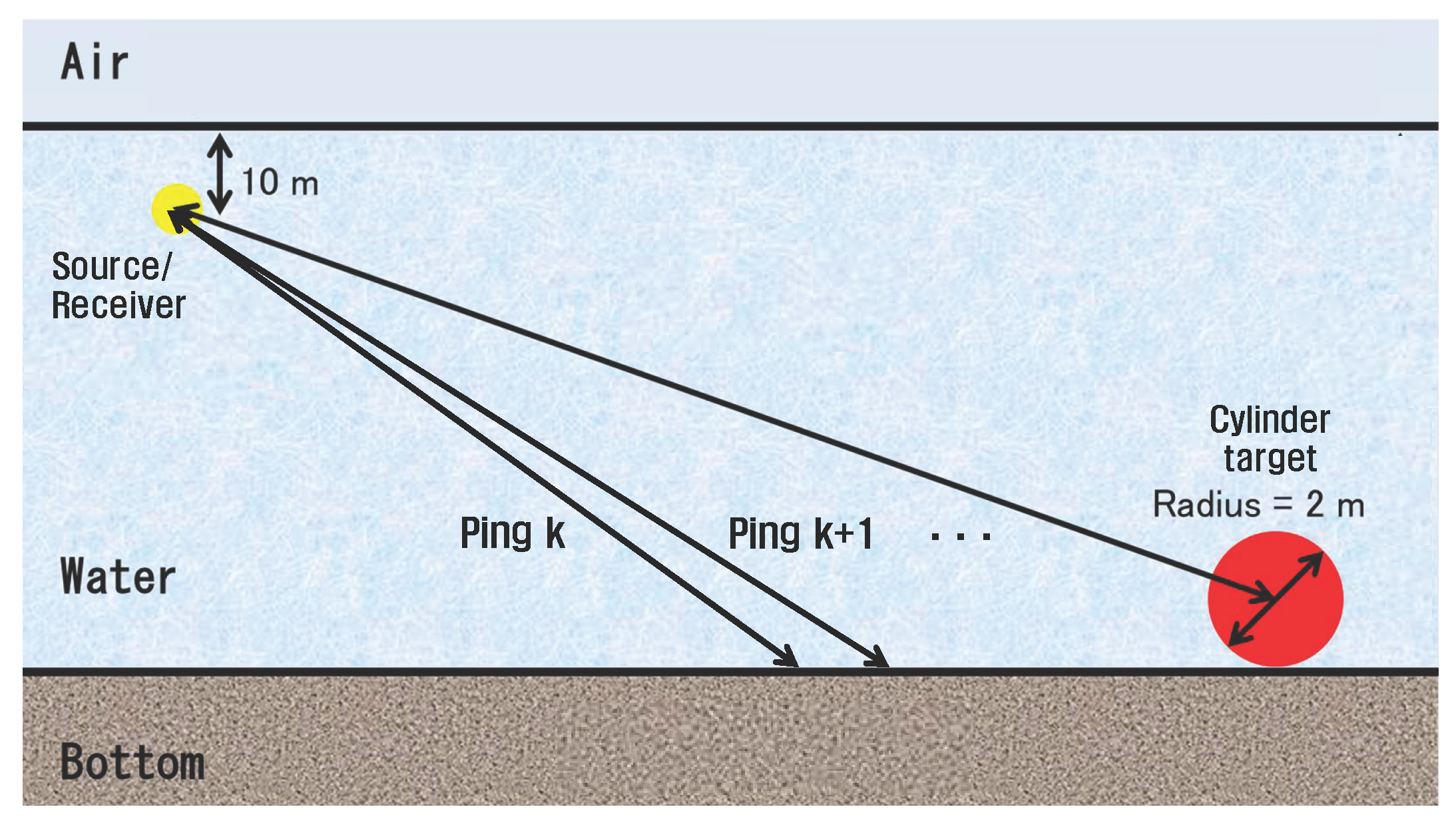
Figure 2.
A model for a resolution cell and patches.
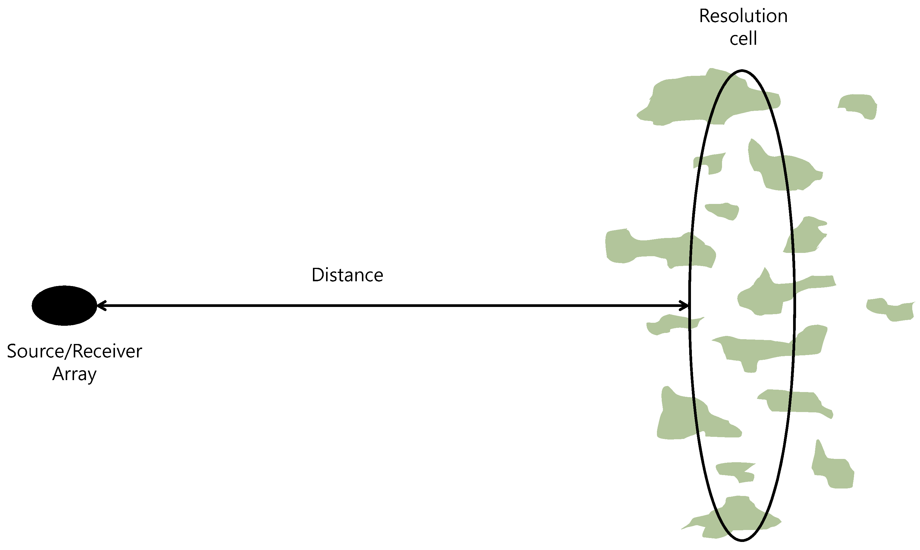
Figure 3.
Target strength of a rigid cylinder with respect to rotation angle.

Figure 4.
Magnitude spectra of the target response for various rotation angles for an linearly frequency modulated (LFM) signal of 13 kHz center frequency and 14 kHz bandwidth.
Figure 4.
Magnitude spectra of the target response for various rotation angles for an linearly frequency modulated (LFM) signal of 13 kHz center frequency and 14 kHz bandwidth.

Figure 5.
Magnitude spectra of the target responses for two grazing angles and two rotation angles.

Figure 6.
Time domain waveforms of the matched filtered received signals with and without a target.
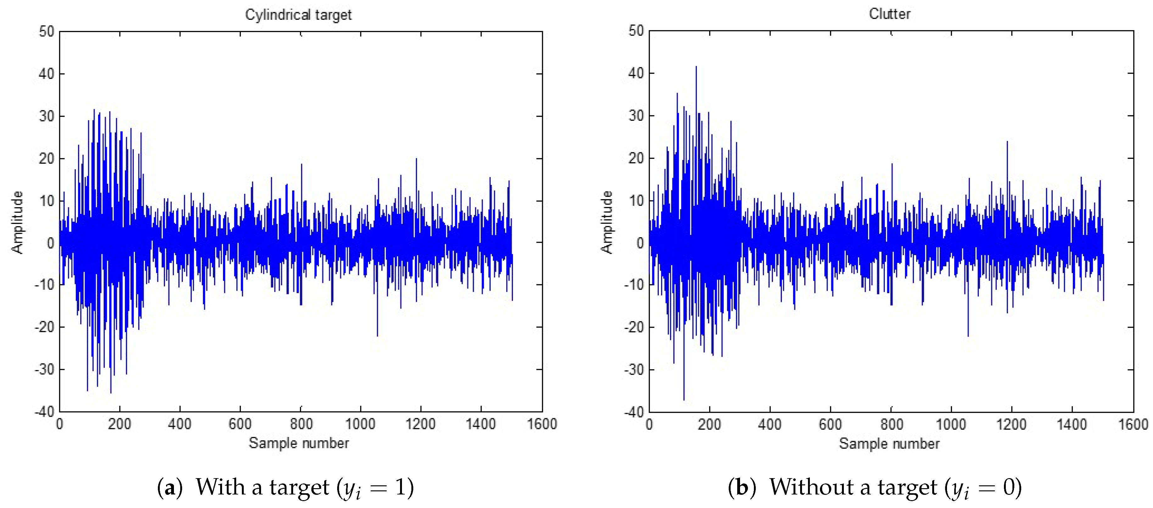
Figure 7.
Magnitude spectra of the match-filtered received signals with and without a target.

Figure 8.
One example of the ten learning parameter s.

Figure 9.
One example of the ten receiver operation characteristic (ROC) curves with average AUC = 0.8983 and its standard deviation = 0.0036. AUC: area under ROC curve.
Figure 9.
One example of the ten receiver operation characteristic (ROC) curves with average AUC = 0.8983 and its standard deviation = 0.0036. AUC: area under ROC curve.
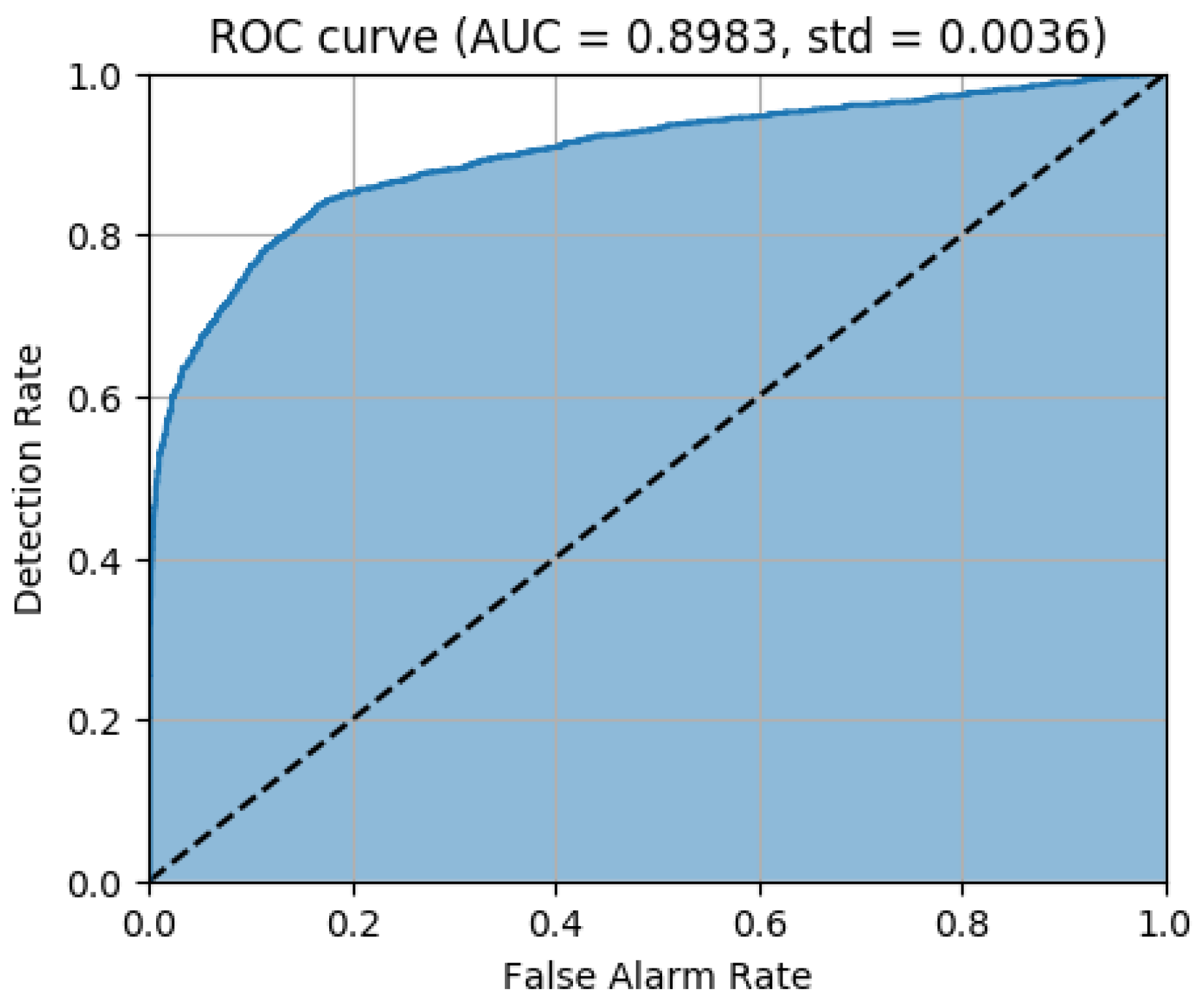
Figure 10.
Learning parameter .
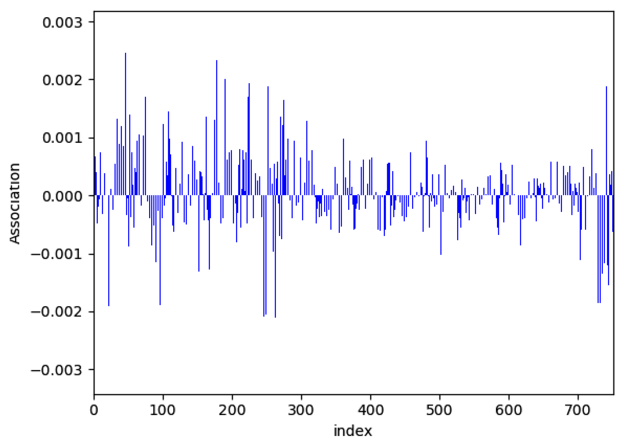
Figure 11.
ROC curve with the learning parameter of Figure 10 for the test data set.
Figure 11.
ROC curve with the learning parameter of Figure 10 for the test data set.

Figure 12.
AUC values with respect to target to clutter ratio (TCR) for the test data set.
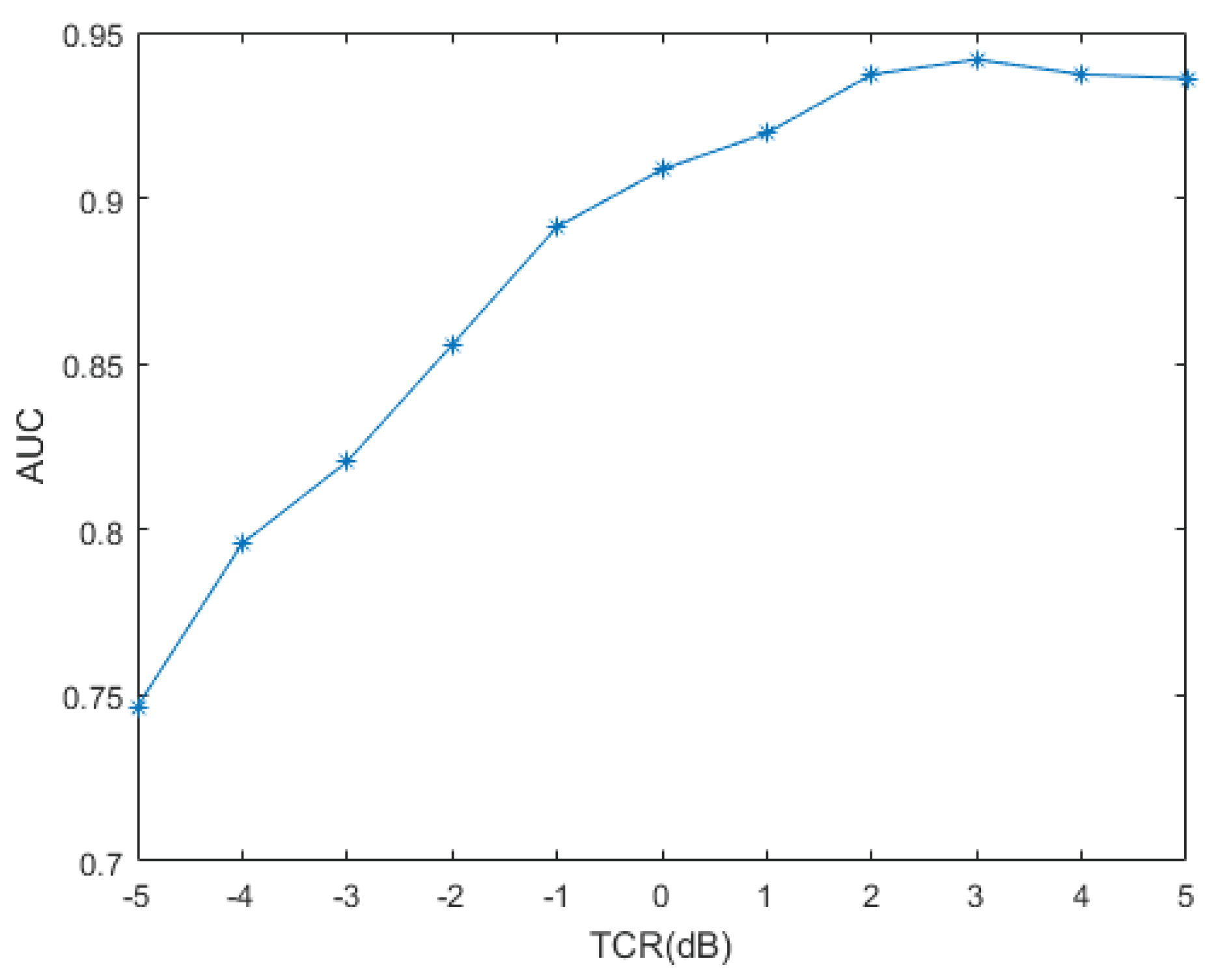
Figure 13.
Probability of detection with respect to TCR for the test data set.

Figure 14.
2D plots of the matched filtered backscattering time series of the three objects at the orientation of 0 degrees (broadside). The dB scale is relative to the brightest pixel in each measurement group. The red lines represent the cross range from −2.5 to 2.5 m, where 400 time series are located.

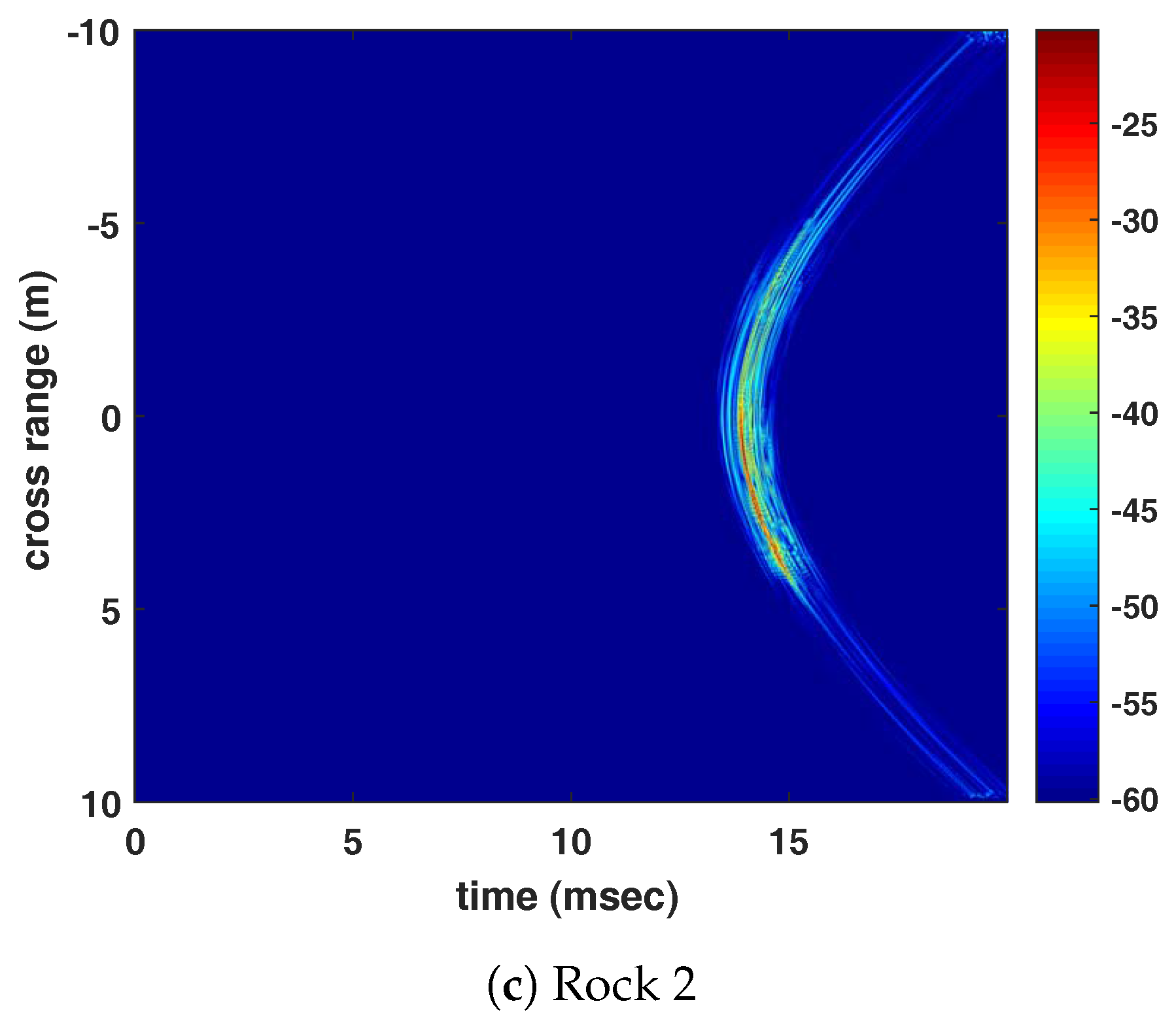
Figure 15.
One example of 1000 ROC curves with average AUC = 0.9325 and its standard deviation = 0.0038.
Figure 15.
One example of 1000 ROC curves with average AUC = 0.9325 and its standard deviation = 0.0038.


Table 1.
Classification table accumulated over the ten trials.
| Predicted Class | ||||
|---|---|---|---|---|
| No Target | Target | Total | ||
| True class | No target | 18,530 | 3640 | 22,170 |
| Target | 3784 | 18,046 | 21,830 | |
| Total | 22,314 | 21,686 | 44,000 | |
Table 2.
Classification table for the model with of Figure 10.
Table 2.
Classification table for the model with of Figure 10.
| Predicted Class | ||||
|---|---|---|---|---|
| No Target | Target | Total | ||
| True class | No target | 4576 | 924 | 5500 |
| Target | 1037 | 4463 | 5500 | |
| Total | 5613 | 5387 | 11,000 | |
Table 3.
List of the coefficients employed to generate the simulated target signals.
| No. | Coef. 2 | Coef.3 | Coef. 2 | Coef. 3 | Coef. 2 | Coef. 3 |
|---|---|---|---|---|---|---|
| 1 | 0.4 | 0.4 | 0.35 | 0.4 | 0.3 | 0.4 |
| 2 | 0.45 | 0.45 | 0.4 | 0.45 | 0.35 | 0.45 |
| 3 | 0.5 | 0.5 | 0.45 | 0.5 | 0.4 | 0.5 |
| 4 | 0.55 | 0.55 | 0.5 | 0.55 | 0.45 | 0.55 |
| 5 | 0.6 | 0.6 | 0.55 | 0.6 | 0.5 | 0.6 |
| 6 | 0.65 | 0.65 | 0.6 | 0.65 | 0.55 | 0.65 |
| 7 | 0.7 | 0.7 | 0.65 | 0.7 | 0.6 | 0.7 |
| 8 | 0.75 | 0.75 | 0.7 | 0.75 | 0.65 | 0.75 |
| 9 | 0.8 | 0.8 | 0.75 | 0.8 | 0.7 | 0.8 |
| 10 | 0.85 | 0.85 | 0.8 | 0.85 | 0.75 | 0.85 |
| 11 | 0.9 | 0.9 | 0.85 | 0.9 | 0.8 | 0.9 |
Table 4.
Classification table of the model with the test data for 1000 simulations.The numbers in parentheses indicate the standard deviation.
Table 4.
Classification table of the model with the test data for 1000 simulations.The numbers in parentheses indicate the standard deviation.
| Predicted Class | ||||
|---|---|---|---|---|
| No Target | Target | Total | ||
| True class | No target | 3479.773 (19.8751) | 120.227 (19.8751) | 3600 |
| Target | 568.718 (29.0805) | 1951.282 (29.0805) | 2520 | |
| Total | 4048.491 | 2071.509 | 6120 | |
© 2018 by the authors. Licensee MDPI, Basel, Switzerland. This article is an open access article distributed under the terms and conditions of the Creative Commons Attribution (CC BY) license (http://creativecommons.org/licenses/by/4.0/).
Share and Cite
MDPI and ACS Style
Seo, Y.; On, B.; Im, S.; Shim, T.; Seo, I. Underwater Cylindrical Object Detection Using the Spectral Features of Active Sonar Signals with Logistic Regression Models. Appl. Sci. 2018, 8, 116. https://doi.org/10.3390/app8010116
AMA Style
Seo Y, On B, Im S, Shim T, Seo I. Underwater Cylindrical Object Detection Using the Spectral Features of Active Sonar Signals with Logistic Regression Models. Applied Sciences. 2018; 8(1):116. https://doi.org/10.3390/app8010116
Chicago/Turabian StyleSeo, Yoojeong, Baeksan On, Sungbin Im, Taebo Shim, and Iksu Seo. 2018. "Underwater Cylindrical Object Detection Using the Spectral Features of Active Sonar Signals with Logistic Regression Models" Applied Sciences 8, no. 1: 116. https://doi.org/10.3390/app8010116
Note that from the first issue of 2016, this journal uses article numbers instead of page numbers. See further details here.