Prescribed Performance Constraint Regulation of Electrohydraulic Control Based on Backstepping with Dynamic Surface

Abstract

In electro-hydraulic system (EHS), uncertain nonlinearities such as some hydraulic parametric uncertainties and external load disturbance often degrade the output dynamic performance. To address this problem, a prescribed performance constraint (PPC) control method is adopted in EHS to restrict the tracking position error of the cylinder position to a prescribed accuracy and guarantee the dynamic and steady position response in a required boundedness under these uncertain nonlinearities. Furthermore, a dynamic surface is designed to avoid the explosion of complexity due to the repeatedly calculated differentiations of the virtual control variables derived in backstepping. The effectiveness of the proposed controller has been verified by a comparative results.

1. Introduction

Electro-hydraulic systems are currently widely used in mechatronic control engineering as they have a superior load efficiency. It was found that EHS starts to be commonly applied for large power systems such as wheel loaders [1], fatigue test devices [2], load simulators [3] and exoskeletons [4]. However, there exist uncertain nonlinearities including parametric uncertainty and external load disturbance in EHS. The former is caused by unknown viscous damping, load stiffness, variations in control fluid volumes, physical characteristics of valve, bulk modulus and oil temperature variations existed in EHS [5,6]. Thus, the high-quality dynamic performance of EHS cannot be always maintained. While the latter is often presented as the driven force or torque of mechanical plant and bias the load pressure of EHS [7]. Thus, the performance holding of EHS under these uncertain nonlinearities is still a challenge problem in EHS control loop. By the way, the parametric uncertainty and noise disturbance also obviously exist in pneumatic system such as mechanical ventilation [8,9,10,11,12,13,14,15,16,17], network distributed control plant [18,19], multiple-input single-output processes [20].

The output-constrained control is welcomed in practice, since the required dynamic behavior can be maintained in the case of different disturbance and uncertainty. Tee and Ge [21,22] originated the barrier Lyapunov function (BLF) to describe the dissipative energy instead of the quadratic Lyapunov function. Then He [23,24,25,26] and Ren [27] employed BLF in general nonlinear system, manipulator and rehabilitation robot. Subsequently, Won [28] proposed backstepping based on BLF with disturbance observer in EHS. Qiu [29] presented backstepping control with dynamic surface for anti-skid braking system. Guo [30] presented a state-constrained controlled by BLF to restrict the position tracking error to a prescribed accuracy and guarantee the load pressure in the maximal power boundary. The merit of BLF is to constrain the system output in the satisfactory boundary by the logarithm transformation of the equivalent output error. However, since the output constraint boundary by BLF is often a constant not a time-varying constraint, the control saturation and chatter output response will emerge in initial time due to the initial large state error, as the boundary is selected very small. Thus, to relax this problem, the prescribed performance constraint (PPC) is initiated by Bechlioulis [31] to guarantee the satisfactory error response and overcome the controllability loss due to the input saturation. Then, Zhang [32,33] used PPC to restrict the attack-of-angle of hypersonic aircraft and the electromechanical system position. In fact, the servo valve control in EHS has limited throttle constraint, which indicates the oversized control will degrade the performance and the stable margin of EHS. The PPC technique transform the original constrained system into a free-constraint model by a designed weighted performance function, which can address both static and time-varying constraints by the regulation of the parameters of weighted performance function.

There exists a potential problem in the common backstepping method, i.e., the explosion of complexity of high-order nonlinear system [34,35] due to the repeatedly calculated differentiations of the virtual control variables emerged in backstepping iteration. These high-order derivatives will magnify noise and uncertainty in the actual control signals which results into violent control and chatter response [32,36]. To solve this problem, the dynamic surface control (DSC) has been proposed to design a stabilizing function instead of the repeatedly calculated derivative of virtual control. The purpose of DSC is to not only eliminate the severe proliferation and system singularity and but also guarantee fast convergence and satisfactory dynamic behavior [29].

In this study, to refuse the negative effect of the external load and hydraulic parametric uncertainty, a novel prescribed performance constraint control is proposed in the position control loop of EHS to constrain the position tracking error to a desirable performance. Different from the constraint holding technique of BLF, the PPC employed a weighted performance function to design an adjustable time-varying output-constraint and improve the system stable margin and dynamic performance. By this controller, all the signals of the single-rod EHS are uniformly bounded and the tracking error of the cylinder position can converge to a small compact set without violating the constraints. Furthermore, the dynamic surface is used to design a stabilizing functions instead of the virtual control derivative in backstepping iteration to avoid violent control and chatter response. Both theoretical proof and comparative results have been provided to verify the effectiveness of the proposed method.

The remainder of this paper is organized as follows. The plant is described in Section 2. The output-constrained controller is given in Section 3 including PPC technique and dynamic surface design. The comparative results of two controllers are given in Section 4. Finally, the conclusion is drawn in Section 5.

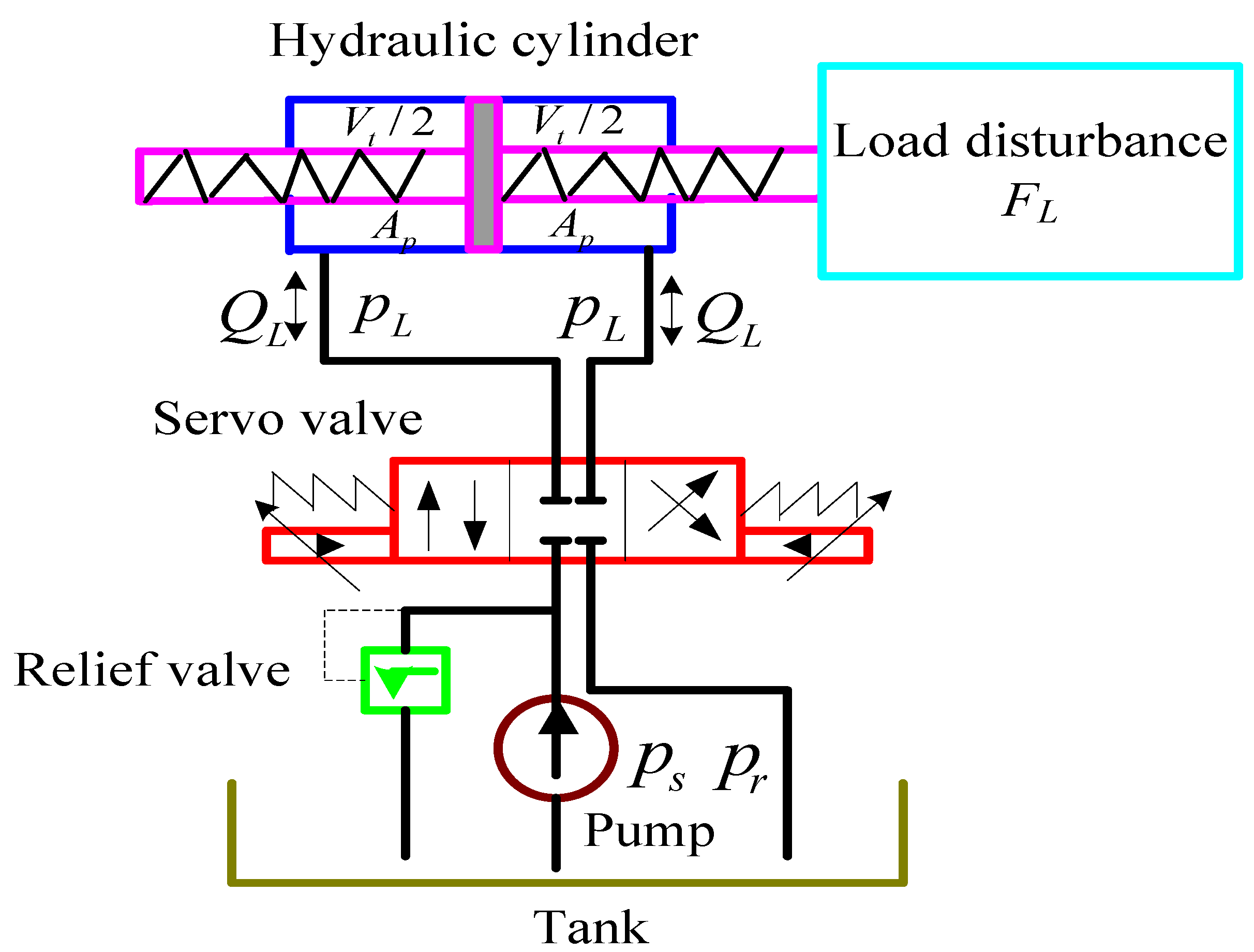
2. Plant Description

The EHS is composed of a servo valve, a symmetrical cylinder, a fixed displacement pump, a motor, and a relief valve as shown in Figure 1. The external load on this EHS is a driven force or torque of any mechatronic plant. The pump outputs the supply pressure $p_s$, which is also the pressure threshold of the relief valve.

Hypothesis 1.

Since the cut-off frequency of servo valve is far greater than the control system bandwidth, the valve dynamics can be neglected in EHS model construction as $x_v=K_{sv}u$, where $x_v$ is the spool position of servo valve, u is the control voltage of servo valve, $K_{sv}$ is the gain of the servo valve [37].

According to Hypothesis 1, if the three state variables are defined as ${[x_1,x_2,x_3]}^T={[y,\dot{y},p_L]}^T$ where y and $\dot{y}$ are the cylinder position and velocity, $p_L$ is the load pressure of the hydraulic cylinder, then the state space model of the EHS is given by

$$\left\{\begin{array}{c}\begin{array}{cc}\hfill {\dot{x}}_1& =x_2\hfill \\ \hfill {\dot{x}}_2& =\frac{1}{m}(A_p{x}_3-K{x}_1-b{x}_2-F_L)\hfill \\ \hfill {\dot{x}}_3& =-\frac{4{\beta }_e{A}_p}{V_t}{x}_2-\frac{4{\beta }_e{C}_{tl}}{V_t}{x}_3+\frac{4{\beta }_e{C}_{d}w{K}_{sv}u}{V_t\sqrt{\rho }}\sqrt{p_s-\mathrm{sgn}\left(u\right)x_3}\hfill \end{array}\end{array}\right.$$

(1)

where $C_d$ is the discharge coefficient, w is the area gradient of the servo valve, $\rho$ is the density of the hydraulic oil, $C_{tl}$ is the coefficient of the total leakage of the cylinder, ${\beta }_e$ is the effective bulk modulus, $A_p$ is the annulus area of the cylinder chamber, $V_t$ is the half-volume of cylinder, m is the load mass, K is load spring constant, b is the viscous damping coefficient of the hydraulic oil, $F_L$ is the external load on the EHS, sgn(·) is the sign function.

Remark 1.

In practice, the hydraulic parameters $C_d$, ρ, w, b, ${\beta }_e$, $C_{tl}$ are usually uncertain constants, but the other parameters are known [38,39].

Remark 2.

The external load $F_L$ is unknown dynamic variable, which is caused by the driving force of someone mechatronic plant. Although the dynamic value of $F_L$ depends on the variables $y,\dot{y},\ddot{y}$, $F_L$ is bounded by $\left|F_L\left(t\right)\right|\le F_{L\max }$, where $F_{L\max }$ is an unknown bounded constant [40,41].

Thus from Remarks 1 and 2, the state space model (1) is rewritten as follow

$$\left\{\begin{array}{c}\begin{array}{cc}\hfill {\dot{x}}_1& =x_2\hfill \\ \hfill {\dot{x}}_2& ={\bar{f}}_2(x_1,x_2)+{\bar{g}}_2{x}_3+{\Delta }_2(x_1,x_2)\hfill \\ \hfill {\dot{x}}_3& ={\bar{f}}_3(x_2,x_3)+{\bar{g}}_3(x_3,u)u+{\Delta }_3(x_1,x_2,x_3)\hfill \end{array}\end{array}\right.,$$

(2)

where ${\bar{C}}_d$, $\bar{\rho }$, $\bar{K}$, $\bar{b}$, ${\bar{\beta }}_e$, ${\bar{C}}_{tl}$ are nominal values of these uncertain parameters respectively,

$$\begin{array}{c}\begin{array}{cc}\hfill {\bar{f}}_2(x_1,x_2)& =-\frac{\bar{K}{x}_1+\bar{b}{x}_2}{m},{\bar{g}}_2=\frac{A_p}{m}\hfill \\ \hfill {\bar{f}}_3(x_2,x_3)& =-\frac{4{\bar{\beta }}_e{A}_p}{V_t}{x}_2-\frac{4{\bar{\beta }}_e{\bar{C}}_{tl}}{V_t}{x}_3\hfill \\ \hfill {\bar{g}}_3(x_3,u)& =\frac{4{\bar{\beta }}_e{\bar{C}}_{d}w{K}_{sv}}{V_t\sqrt{\bar{\rho }}}\sqrt{p_s-\mathrm{sgn}\left(u\right)x_3}\hfill \end{array}\end{array},$$

(3)

and ${\Delta }_2(x_1,x_2)=f_2(x_1,x_2)-{\bar{f}}_2(x_1,x_2)-F_L\left(t\right)/m$, ${\Delta }_3(x_1,x_2,x_3)=f_3(x_2,x_3)-{\bar{f}}_3(x_2,x_3)+g_3(x_1,x_2,x_3)-{\bar{g}}_3(x_1,x_2,x_3)$ are the integrated elements of parametric uncertainties and the external load disturbance.

Due to limited boundaries of the parametric uncertainties and the external load mentioned in Remarks 1 and 2, the two uncertain nonlinearities ${\Delta }_2$, ${\Delta }_3$ are bounded by $\left|{\Delta }_2\right|<{\Delta }_{2\max }$, $\left|{\Delta }_3\right|<{\Delta }_{3\max }$, where ${\Delta }_{2\max }$, ${\Delta }_{3\max }$ are unknown bounded constants [28].

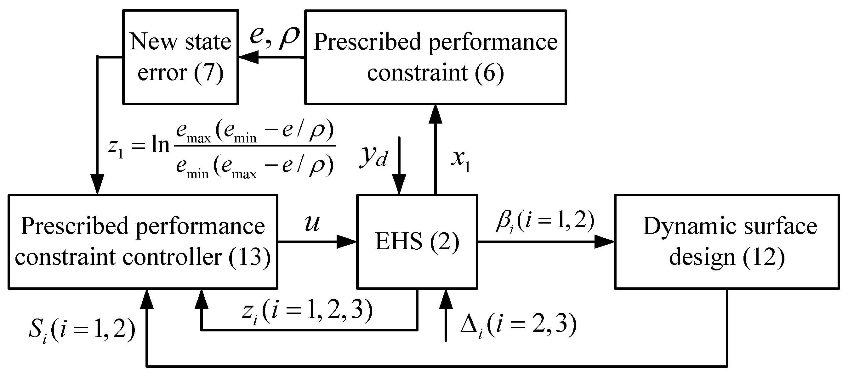
3. Prescribed Performance Constraint Control of EHS

3.1. Prescribed Performance Constraint

The prescribed performance constraint of position tracking error is regulated by a designed weighted performance function, which can guarantee not only the satisfactory dynamic performance but also the stable margin of EHS.

At first, the position tracking error is given by

$$e\left(t\right)=x_1\left(t\right)-y_d\left(t\right).$$

(4)

If the cylinder position $x_1$ is restricted in $x_{1\min }<x_1\left(t\right)<x_{1\max }$, where $x_{1\min }$ and $x_{1\max }$ are the maximal and minimal boundary of $x_1$, and the position demand $y_d$ has also two definite boundaries as $y_{d\min }\le y_d\le y_{d\max }$, then

$$e_{\min }<e\left(t\right)<e_{\max },$$

(5)

where $e_{\min }=x_{1\min }-y_{d\max }$, $e_{\max }=x_{1\max }-y_{d\min }$.

Definition 1.

A continuous smooth function [32] $\rho \left(t\right)=(\rho \left(0\right)-\rho (\infty ))e^{-\lambda t}+\rho (\infty )$ is called a weighted performance function if

(1) 

$\rho \left(t\right)$ is positive and monotonically decreasing;

(2) 

$\underset{x\to \infty }{\lim }\rho \left(t\right)={\rho }_{\infty }>0$;

(3) 

$\rho (\infty )<\rho \left(0\right)<1$.

Lemma 1.

If a weighted performance function $\rho \left(t\right)$ is designed such that

$$e_{\min }<e\left(t\right)/\rho \left(t\right)<e_{\max },$$

(6)

then $e\left(t\right)$ is restricted in $(e_{\min },e_{\max })$ [31].

Actually, if $e\left(t\right)\ge 0$, then $e\left(t\right)\le e\left(t\right)/{\rho }_i\left(t\right)<e_{\max }$ due to $0<{\rho }_i\left(t\right)<1$. On the other hand, if $e\left(t\right)<0$, then $e_{\min }<e\left(t\right)/\rho \left(t\right)<e\left(t\right)$. Thus, the position tracking error $e\left(t\right)$ is always restricted in the boundaries $(e_{\min },e_{\max })$.

Secondly, according to Lemma 1, the PPC $\rho \left(t\right)e_{\min }<e\left(t\right)<\rho \left(t\right)e_{\max }$ can derive a new state errors as follow

$$z_1\left(t\right)=T^{-1}\left(\frac{e\left(t\right)}{\rho \left(t\right)}\right)=ln\left(\frac{e_{\max }(e_{\min }-e\left(t\right)/\rho \left(t\right))}{e_{\min }(e_{\max }-e\left(t\right)/\rho \left(t\right))}\right),$$

(7)

where $T(·)$ is a smooth function, $T^{-1}(·)$ is its inverse function, $ln(·)$ is the natural logarithm function.

Theorem 1.

The smooth function $T(·)$ is a monotonically increasing function [33], and holds the following properties

$$\begin{array}{c}\begin{array}{c}\begin{array}{cc}\hfill e_{\min }<& T\left(z_1\right)<e_{\max }T\left(0\right)=0\hfill \\ \hfill \underset{z_1\to -\infty }{\lim }& T\left(z_1\right)=e_{\min }\underset{z_1\to +\infty }{\lim }T\left(z_1\right)=e_{\max }\hfill \end{array}\hfill \end{array}\end{array}.$$

(8)

Proof. 

From (33), the inverse function of $z_1$ is given by

$$T\left(z_1\right)=\frac{e\left(t\right)}{\rho \left(t\right)}=\frac{e_{\min }{e}_{\max }(e^{z_1}-1)}{e_{\min }{e}^{z_1}-e_{\max }}.$$

(9)

Since $e_{\min }<0$ and $e_{\max }>0$, the derivative of $T\left(z_1\right)$ yields

$$\frac{dT}{d{z}_1}=\frac{e_{\min }(e_{\min }-e_{\max })e^{z_1}}{{(e_{\min }{e}^{z_1}-e_{\max })}^2}>0.$$

(10)

Hence, $T\left(z_1\right)$ is a monotonically increasing function. Furthermore, due to $\rho \left(t\right)e_{\min }<e\left(t\right)<\rho \left(t\right)e_{\max }$ with $0<\rho \left(t\right)<1$, then $e_{\min }<T\left(z_1\right)<e_{\max }$ is established. When $z_1\to \pm \infty$, $T\left(z_1\right)$ is close to its up and down boundary $e_{\max }$ and $e_{\min }$ respectively. If $z_1=0$ is substituted into (7), then $T\left(0\right)=0$. ☐

3.2. Controller Design Based on PPC

Together with (7), the system state errors are defined as follows

$$\left\{\begin{array}{c}\begin{array}{cc}\hfill z_1& =ln\left(\frac{e_{\max }(e_{\min }-e/\rho )}{e_{\min }(e_{\max }-e/\rho )}\right)\hfill \\ \hfill z_2& =x_2-{\alpha }_1\hfill \\ \hfill z_3& =x_3-{\alpha }_2\hfill \end{array}\end{array}\right.,$$

(11)

where e is the position tracking error defined in (4), ${\alpha }_i(i=1,2)$ is the virtual control variable in controller design.

To avoid the explosion of complexity caused by the repeatedly calculated differentiations of ${\dot{\alpha }}_i(i=1,2)$ in the backstepping iteration, the dynamic surfaces of $z_{i+1}(i=1,2)$ are given as follows

$$\begin{array}{cc}{\tau }_i{\dot{\alpha }}_i+{\alpha }_i={\beta }_i,\hfill & {\alpha }_i\left(0\right)={\beta }_i\left(0\right)\hfill \end{array}$$

(12)

where ${\beta }_i(i=1,2)$ are the stabilizing functions to be designed, ${\tau }_i(i=1,2)$ are the time constants of the dynamic surfaces.

Thus, the output errors of two dynamic surfaces are defined as $S_i={\alpha }_i-{\beta }_i(i=1,2)$ . Substituting $S_i$ into (12), the virtual control derivatives ${\dot{\alpha }}_i=-S_i/{\tau }_i(i=1,2)$ are obtained.

Based on the system state errors (11) and the dynamic surface (12), the prescribed performance constraint controller u is designed as follow

$$\left\{\begin{array}{c}\begin{array}{cc}\hfill {\beta }_1& ={\dot{y}}_d+\frac{\dot{\rho }}{\rho }e-k_1\frac{z_1}{r}\hfill \\ \hfill {\beta }_2& =-\frac{1}{{\bar{g}}_2}\left(k_2{z}_2+r{z}_1+{\bar{f}}_2+\frac{S_1}{{\tau }_1}\right)\hfill \\ \hfill {\alpha }_i& =-\underset{0}{\overset{t}{\int }}\frac{S_i}{{\tau }_i}dt,i=1,2\hfill \\ \hfill S_i& ={\alpha }_i-{\beta }_i,i=1,2\hfill \\ \hfill u& =-\frac{1}{{\bar{g}}_3}\left(k_3{z}_3+{\bar{f}}_3+{\bar{g}}_2{z}_2+\frac{S_2}{{\tau }_2}\right)\hfill \end{array}\end{array}\right.,$$

(13)

where the attenuated parameter r is

$$r=\frac{\partial T^{-1}}{\partial (e/\rho )}\frac{1}{\rho }=\frac{e_{\max }-e_{\min }}{(e_{\max }-e/\rho )(e/\rho -e_{\min })\rho }\ge \frac{e_{\max }-e_{\min }}{{\left(\frac{e_{\max }-e_{\min }}{2}\right)}^2}=\frac{4}{e_{\max }-e_{\min }}>0.$$

(14)

Theorem 2.

Considering the stabilizing functions (13) together with their dynamic surfaces (12) for the EHS model (2) under Hypothesis 1 and Remarks 1 and 2, regardless of the system state errors $z_i\left(t\right)(i=1,2,3)$ start from any initial values $-\infty <z_i\left(0\right)<\infty$, the generalized error $Z_g\left(t\right)$ including $z_i(i=1,2,3)$ and $S_j(j=1,2)$ is ultimate boundedness [42] and its convergence domain is an hypersphere $H_r$,

$$H_r\in \left\{\sum _{i=1}^3{z}_i^2+\sum _{j=1}^2{S}_j^2=2V\left(0\right)e^{-c{t}_f}+2\delta /c\right\}$$

(15)

where δ and c are positive constants, $V\left(0\right)$ is the initial system state error, $\forall t>t_f$ ($t_f$ is a finite time).

Proof. 

The candidate quadratic Lyapunov function of the EHS model (2) is given by

$$V=\frac{1}{2}\sum _{i=1}^3{z}_i^2+\frac{1}{2}\sum _{j=1}^2{S}_j^2.$$

(16)

For convenient proof, V is rewritten into the cascade elements for the convenient controller design as follows

$$\left\{\begin{array}{c}\begin{array}{cc}\hfill V_1& =\frac{1}{2}{z}_1^2+\frac{1}{2}{S}_1^2\hfill \\ \hfill V_2& =V_1+\frac{1}{2}{z}_2^2+\frac{1}{2}{S}_2^2\hfill \\ \hfill V_3& =V_2+\frac{1}{2}{z}_3^2\hfill \end{array}\end{array}\right.,$$

(17)

and the following inequalities are satisfied by Young’s inequality

$$\begin{array}{c}\left|z_i{S}_i\right|\le \frac{z_i^2+S_i^2}{2}\left|S_i{\dot{\beta }}_i\right|\le \frac{S_i^2{\left|{\dot{\beta }}_i\right|}_{\max }^2}{2{\sigma }_i}+\frac{{\sigma }_i}{2}\left|z_{i+1}{\Delta }_{i+1}\right|\le \frac{z_{i+1}^2+{\Delta }_{i+1\max }^2}{2}\end{array},$$

(18)

for $i=1,2$, where ${\sigma }_i(i=1,2)$ are positive constants, ${\left|{\dot{\beta }}_i\right|}_{\max }(i=1,2)$ are the maximal boundaries of ${\dot{\beta }}_i(i=1,2)$.

Step 1: Substituting (2), (11), (12) into the derivative of $V_1$, ${\dot{V}}_1$ yields

$$\begin{array}{c}\begin{array}{cc}\hfill {\dot{V}}_1& =z_1{\dot{z}}_1+S_1{\dot{S}}_1=z_{1}r(x_2-{\dot{x}}_{1d}-\frac{e\left(t\right)}{\rho \left(t\right)}\dot{\rho }\left(t\right))+S_1({\dot{\alpha }}_1-{\dot{\beta }}_1)\hfill \\ & =z_{1}r(z_2+{\beta }_1+S_1-{\dot{x}}_{1d}-\frac{e\left(t\right)}{\rho \left(t\right)}\dot{\rho }\left(t\right))+S_1(-\frac{S_1}{{\tau }_1}-{\dot{\beta }}_1)\hfill \end{array}\hfill \end{array}$$

(19)

If the stabilizing function ${\beta }_1$ in (13) is substituted into (19), and together with (18), then ${\dot{V}}_1$ is converted to

$$\begin{array}{c}\begin{array}{c}\begin{array}{cc}\hfill {\dot{V}}_1& ={\bar{\dot{V}}}_1+\frac{{\sigma }_1}{2}+r{z}_1{z}_2\hfill \\ \hfill {\bar{\dot{V}}}_1& =-{\mathsf{\Gamma }}_1{z}_1^2-{\mathsf{\Omega }}_1{S}_1^2\hfill \end{array}\hfill \end{array}\hfill \end{array},$$

(20)

where

$${\mathsf{\Gamma }}_1=k_1-\frac{r}{2},{\mathsf{\Omega }}_1=\frac{1}{{\tau }_1}-\frac{r}{2}-\frac{{\left|{\dot{\beta }}_1\right|}_{\max }^2}{2{\sigma }_1}.$$

(21)

If a constant gain $k_1$ and a time constant ${\tau }_1$ yield such that

$$k_1>\frac{r}{2},\frac{1}{{\tau }_1}>\frac{r}{2}+\frac{{\left|{\dot{\beta }}_1\right|}_{\max }^2}{2{\sigma }_1},$$

(22)

then ${\bar{\dot{V}}}_1<0$.

Step 2: The derivative of $V_2$ is given by

$$\begin{array}{c}\begin{array}{cc}\hfill {\dot{V}}_2& ={\dot{V}}_1+z_2{\dot{z}}_2+S_2{\dot{S}}_2\hfill \\ & \le {\bar{\dot{V}}}_1+\frac{{\sigma }_1}{2}+r{z}_1{z}_2+z_2[{\bar{f}}_2+{\bar{g}}_2(z_3+{\beta }_2+S_2)-{\dot{\alpha }}_1+{\Delta }_2]+S_2({\dot{\alpha }}_2-{\dot{\beta }}_2)\hfill \\ & \le {\bar{\dot{V}}}_1+\frac{{\sigma }_1}{2}+z_2[r{z}_1+{\bar{f}}_2+{\bar{g}}_2(z_3+{\beta }_2+S_2)+\frac{S_1}{{\tau }_1}+{\Delta }_2]+S_2(-\frac{S_2}{{\tau }_2}-{\dot{\beta }}_2)\hfill \end{array}\hfill \end{array}.$$

(23)

If the stabilizing function ${\beta }_2$ in (13) is substituted into (23), and together with (18), then ${\dot{V}}_2$ yields

$$\begin{array}{c}\begin{array}{cc}\hfill {\dot{V}}_2& \le {\bar{\dot{V}}}_2+{\bar{g}}_2{z}_2{z}_3+\frac{{\sigma }_1}{2}+\frac{{\sigma }_2}{2}+\frac{{\Delta }_{2\max }^2}{2}\hfill \\ \hfill {\bar{\dot{V}}}_2& ={\bar{\dot{V}}}_1-{\mathsf{\Gamma }}_2{z}_2^2-{\mathsf{\Omega }}_2{S}_2^2\hfill \end{array}\hfill \end{array},$$

(24)

where

$${\mathsf{\Gamma }}_2=k_2-\frac{{\left|{\bar{g}}_2\right|}_{\max }^2}{2}-\frac{1}{2},{\mathsf{\Omega }}_2=\frac{1}{{\tau }_2}-\frac{{\left|{\bar{g}}_2\right|}_{\max }^2}{2}-\frac{{\left|{\dot{\beta }}_2\right|}_{\max }^2}{2{\sigma }_2}.$$

(25)

Step 3: Similarly, the derivative of $V_3$ is given by

$$\begin{array}{c}\begin{array}{cc}\hfill {\dot{V}}_3& ={\dot{V}}_2+z_3{\dot{z}}_3\hfill \\ & \le {\bar{\dot{V}}}_2+{\bar{g}}_2{z}_2{z}_3+\frac{{\sigma }_1}{2}+\frac{{\sigma }_2}{2}+\frac{{\Delta }_{2\max }^2}{2}+z_3[{\bar{f}}_3+{\bar{g}}_{3}u-{\dot{\alpha }}_2+{\Delta }_3]\hfill \\ & \le {\bar{\dot{V}}}_2+\frac{{\sigma }_1}{2}+\frac{{\sigma }_2}{2}+\frac{{\Delta }_{2\max }^2}{2}+z_3[{\bar{g}}_2{z}_2+{\bar{f}}_3+{\bar{g}}_{3}u+\frac{S_2}{{\tau }_2}+{\Delta }_3]\hfill \end{array}\hfill \end{array}$$

(26)

If the control variable u is designed as the form in (13), then ${\dot{V}}_3$ yields

$${\dot{V}}_3\le {\bar{\dot{V}}}_2-k_3{z}_3^2+\delta ,$$

(27)

where $\delta =({\sigma }_1+{\sigma }_2+{\Delta }_{2\max }^2+{\Delta }_{3\max }^2)/2$ is a positive constant.

If a constant c is defined as $c=\min \{2{\mathsf{\Gamma }}_1,2{\mathsf{\Gamma }}_2,2{\mathsf{\Omega }}_1,2{\mathsf{\Omega }}_2,2k_3\}$, from the definitions of ${\bar{\dot{V}}}_1$ and ${\bar{\dot{V}}}_2$, (27) is rewritten as

$${\dot{V}}_3\le -c{V}_3+\delta .$$

(28)

Integrating (28), ${\dot{V}}_3$ yields

$$\begin{array}{c}\begin{array}{cc}\hfill V\left(t\right)& \le V\left(0\right)e^{-ct}+\underset{0}{\overset{t}{\int }}\delta e^{-c(t-\epsilon )}d\epsilon \hfill \\ & \le V\left(0\right)e^{-ct}+\delta (1-e^{-ct})/c\hfill \end{array}\hfill \end{array}.$$

(29)

According to (29), and letting $t\to t_f$, the error convergence domain $H_r$ in (15) is obtained. Furthermore, the size of the generalized error convergence domain $H_r$ mainly is decided by the element $\delta /c$. Thus, the increased control gains $k_i(i=1,2,3)$ and the reduced constant c can arbitrarily shrink the size of $H_r$ as $t\to \infty$. ☐

Figure 2 shows the proposed prescribed performance constraint controller. The designed dynamic surface (12) is used to instead of the virtual control derivatives ${\dot{\alpha }}_i(i=1,2)$ and the virtual control variables ${\alpha }_i(i=1,2)$ are substituted by the stabilizing functions ${\beta }_i(i=1,2)$. The output-constraint (5) is converted to the time-varying performance constraint (6), which represents the position tracking error e of EHS. Then this constraint is transformed into the new state error $z_1$ (7). The controller u (13) is constructed to guarantee the dynamic performance of the EHS (2) under the hydraulic parametric uncertainties and the external load disturbance integrated in ${\Delta }_i(i=2,3)$.

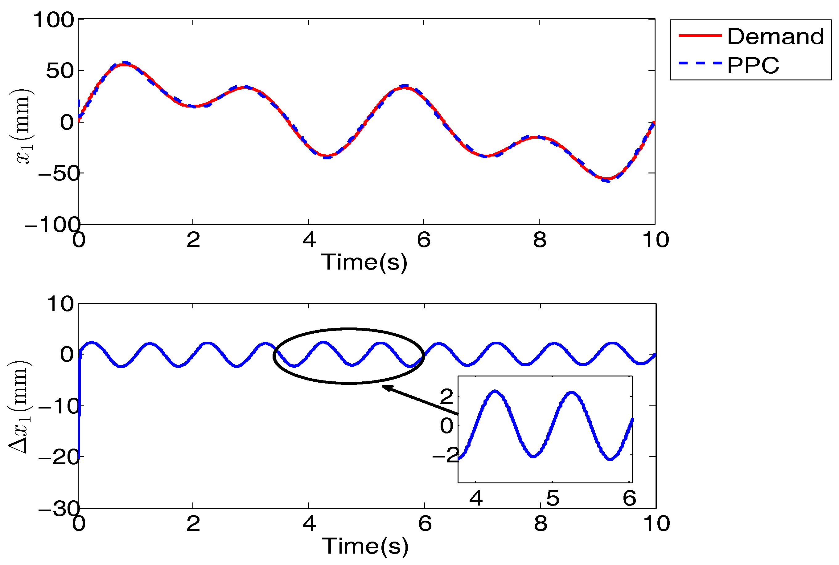
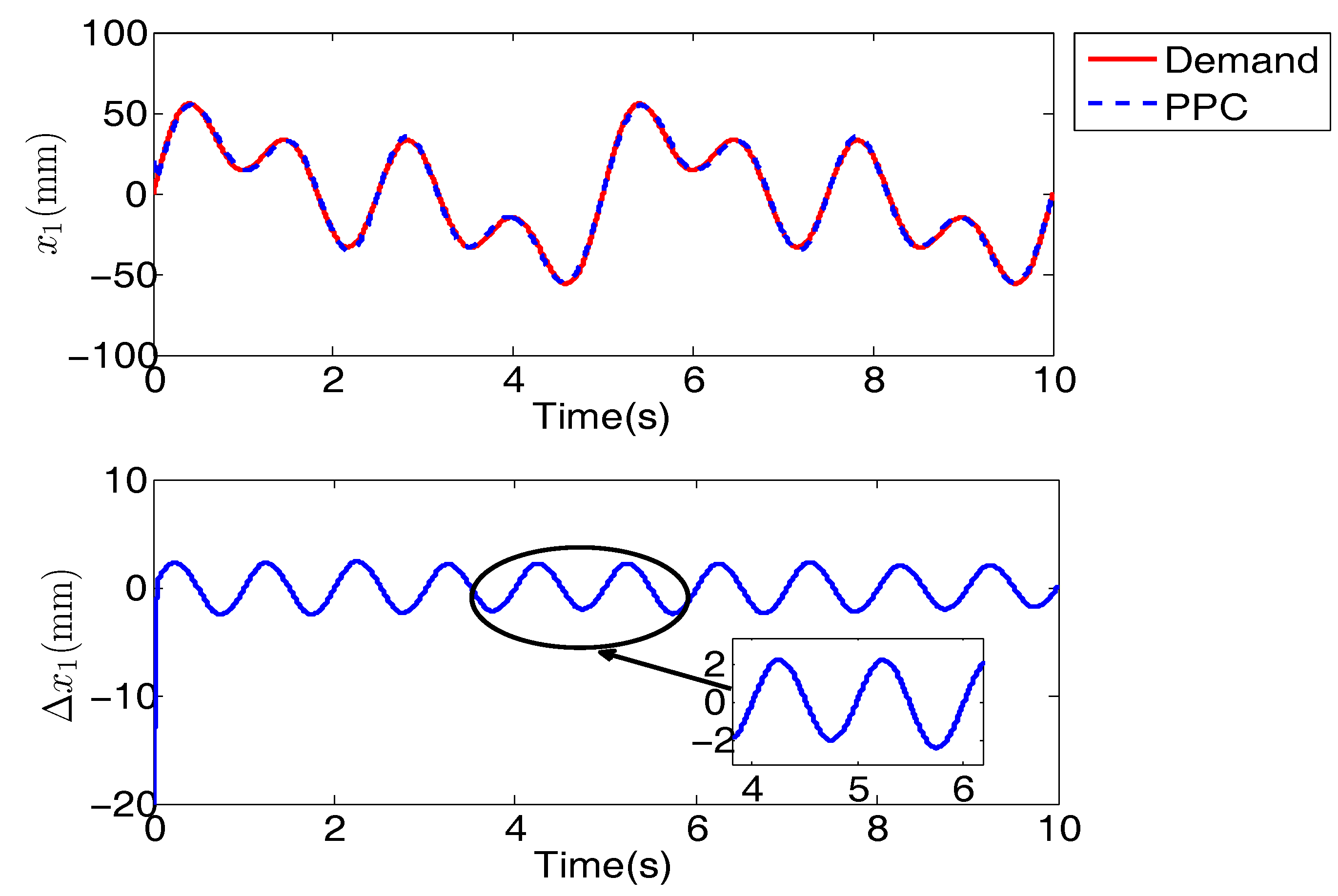
4. Comparison Results

To verify the proposed prescribed performance constraint control method, some known hydraulic parameters are ${\bar{C}}_d=0.62$, $w=0.024$ m, $x_{v\max }=7.9$ mm, ${\bar{\beta }}_e=7000$ bar, $\bar{\rho }=850$ $\mathrm{kg}/{\mathrm{m}}^3$, $\bar{K}=1000$ N/m, $\bar{b}=100$ Ns/m, ${\bar{C}}_{tl}=2.5\times {10}^{-11}{\mathrm{m}}^3/(\mathrm{s}·\mathrm{Pa})$, $K_{sv}=4.9\times {10}^{-6}$ m/V, $p_r=2$ bar, $A_p=2.01{\mathrm{cm}}^2$, $V_t=1.74\times {10}^{-5}{\mathrm{m}}^3$, $m=1.739$ kg, $\Delta C_d=0.1{\bar{C}}_d$, $\Delta {\beta }_e=0.5{\bar{\beta }}_e$, $\Delta K=0.5\bar{K}$, $\Delta b=0.5\bar{b}$, $\Delta \rho =-0.1\bar{\rho }$, $\Delta C_{tl}=0.2{\bar{C}}_{tl}$, $F_{L\max }=500$ N. The time constants of two dynamic surfaces is ${\tau }_1={\tau }_2={10}^{-3}$. Some control parameters are designed as $k_1=100$, $k_2=1200$ and $k_3=6000$, $x_{1\min }=-50$ mm, $x_{1\max }=50$ mm, $y_{\min }=-50$ mm, $y_{\max }=50$ mm, $\rho \left(0\right)=0.95$, $\rho (\infty )=0.03$, $\lambda =0.3$.

In addition, to compare with the traditional control scheme, Proportional-Integral (PI) controller is also adopted in this EHS such that

$$u=k_p(y_d-x_1)+k_i\int (y_d-x_1)dt$$

(30)

where the control gains $k_p$ = 150 and $k_i$ = 10 have been well tuned to guarantee the fast response of the cylinder position.

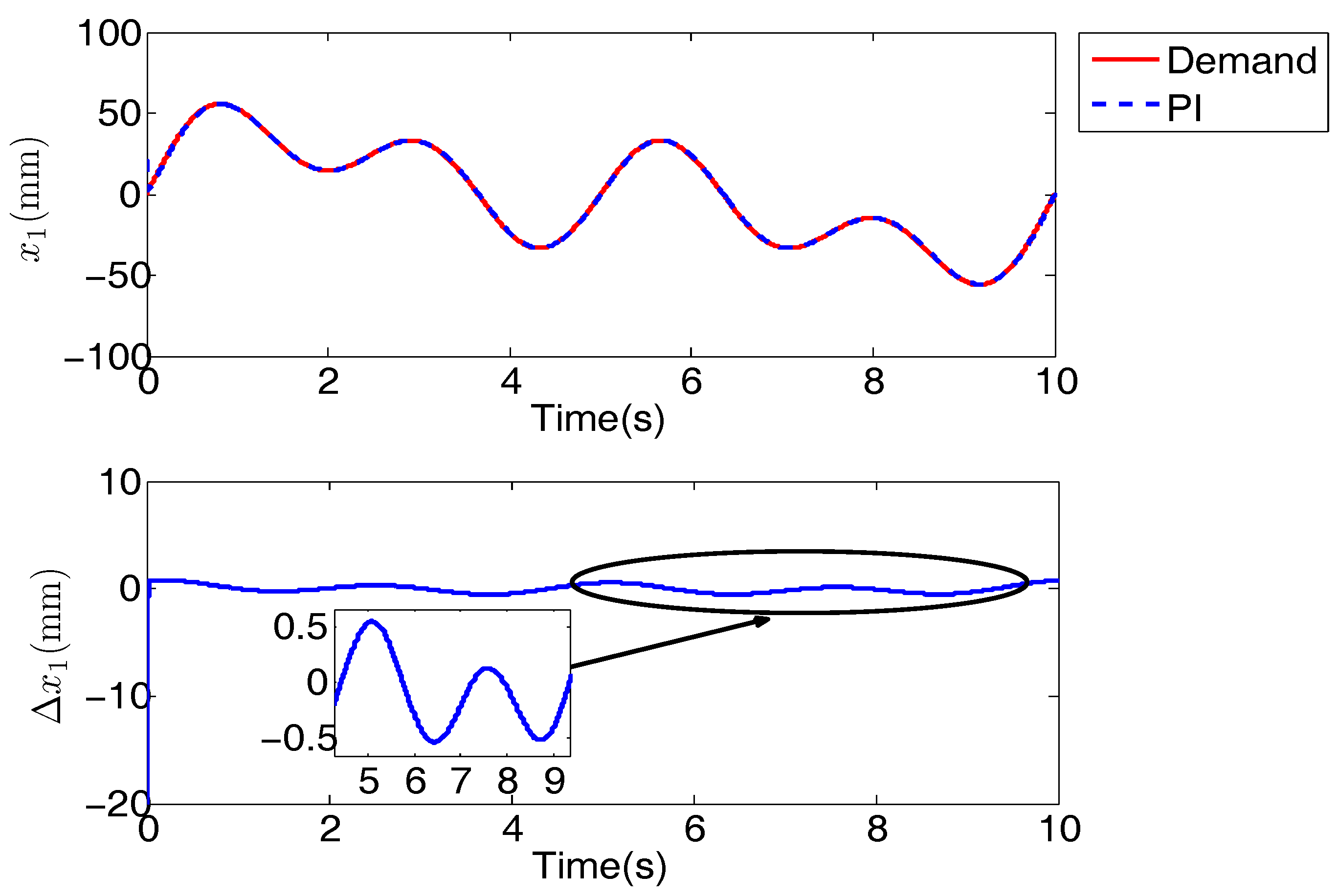
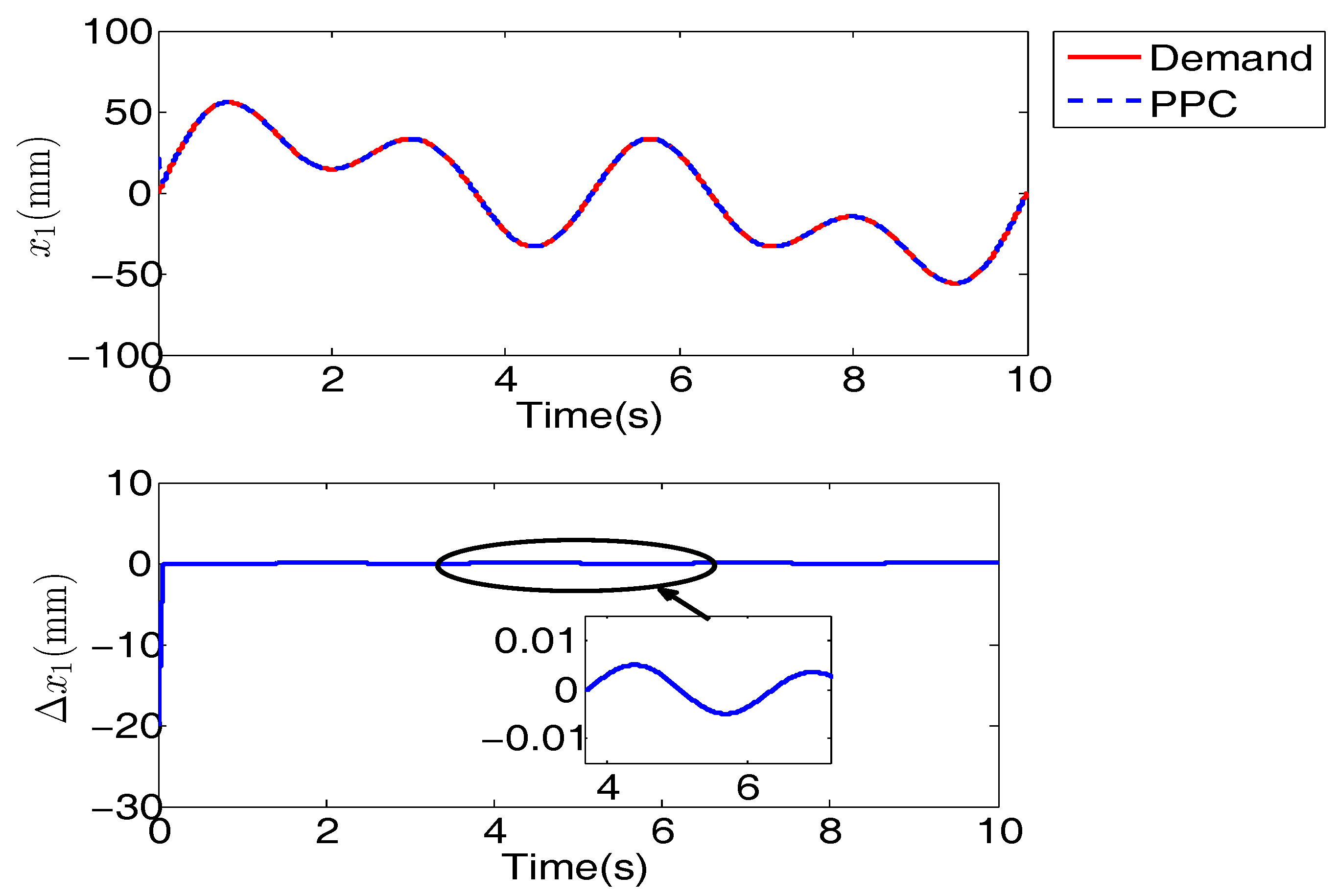
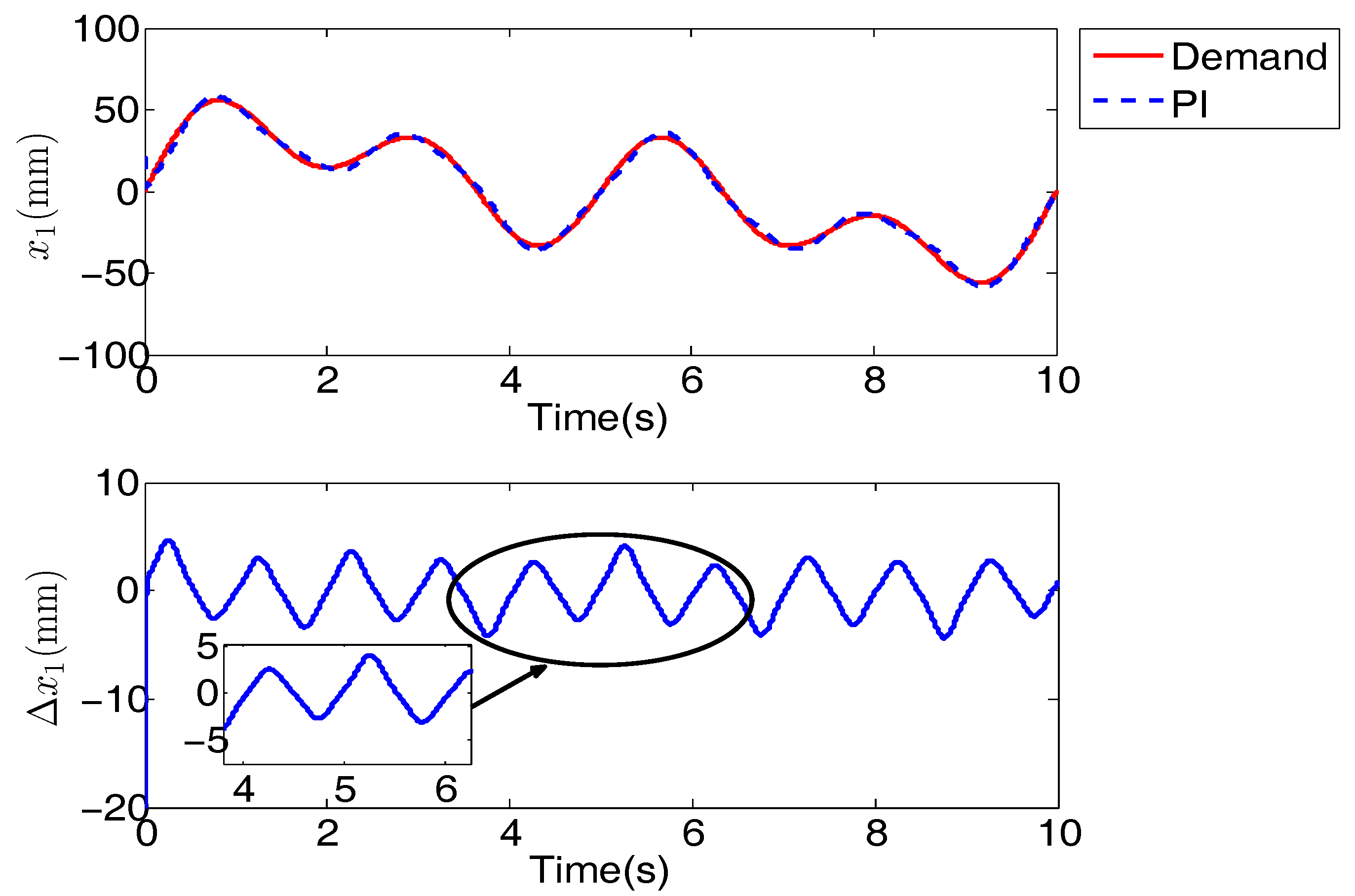
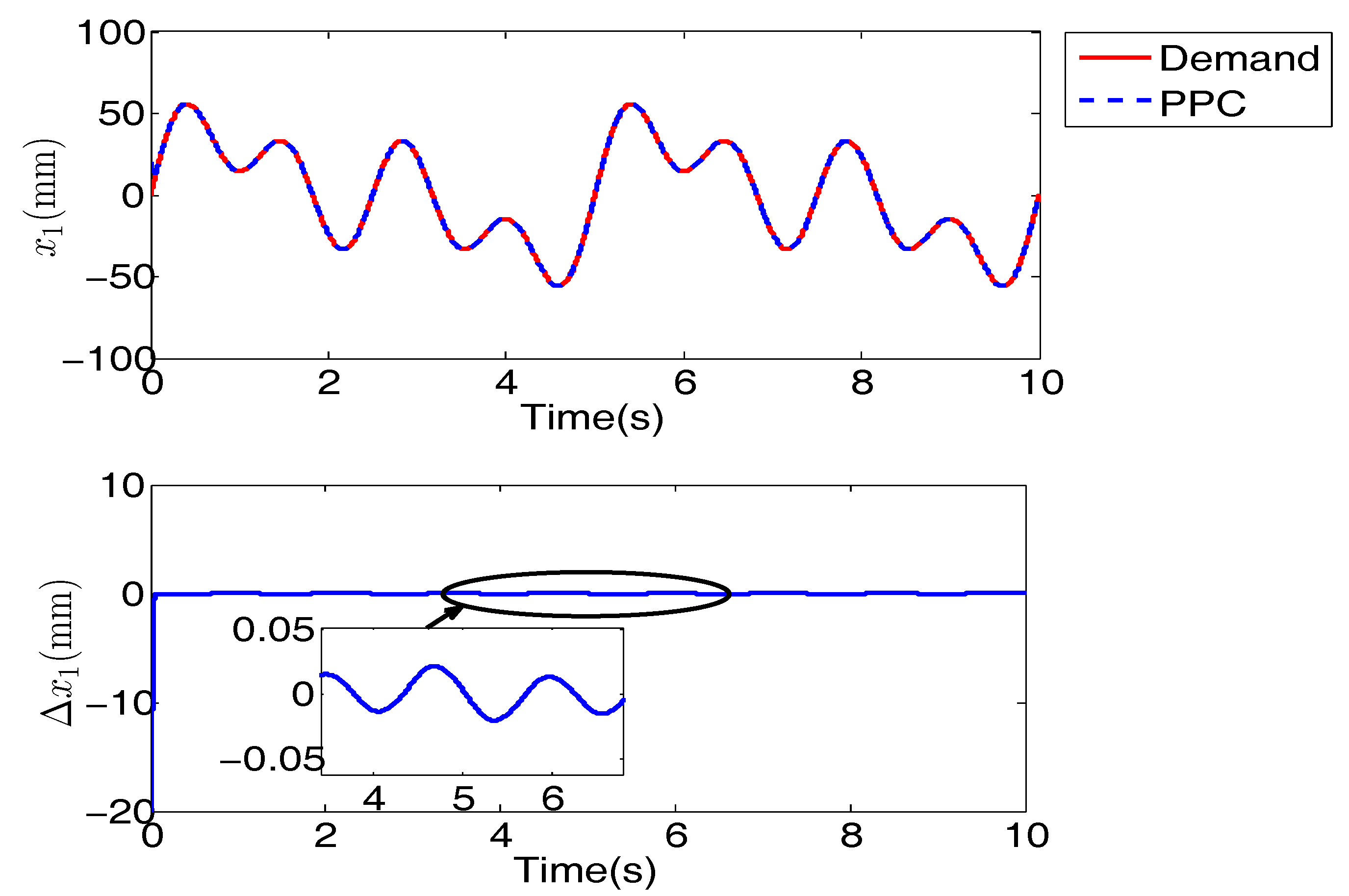
4.1. Compared Results with Nominal Hydraulic Parameters

Firstly, the nominal hydraulic parameters is adopted in simulation with the uncertain nonlinearities ${\Delta }_2={\Delta }_3=0$. The cylinder position demands are selected as $y_d=25(\sin \left(0.8\pi t\right)+\sin \left(0.4\pi t\right)+\sin \left(0.2\pi t\right))$ mm and $y_d=25(\sin \left(1.6\pi t\right)+\sin \left(0.8\pi t\right)+\sin \left(0.4\pi t\right))$ mm. The initial states of two control schemes are $x_1\left(0\right)=20$ mm, $x_2\left(0\right)=0$ mm/s, $x_3\left(0\right)=0$ bar. The proposed controller comparison with PI controller are shown in Figure 3, Figure 4, Figure 5and Figure 6. The controller based on prescribed performance constraint has the steady tracking errors $\Delta x_1=0.01$ mm in low frequency demand and $\Delta x_1=0.05$ mm in high frequency demand respectively, which is better than the PI controller $\Delta x_1=0.5$ mm and $\Delta x_1=2$ mm in corresponding frequency demand. Since the constraint holding technique is adopted in the proposed controller, the tracking error of the cylinder position is not always beyond the prescribed constraint $\rho \left(t\right)e_{\min }<e\left(t\right)<\rho \left(t\right)e_{\max }$. Thus, these comparison results indicate the advantage of this prescribed performance constraint technique.

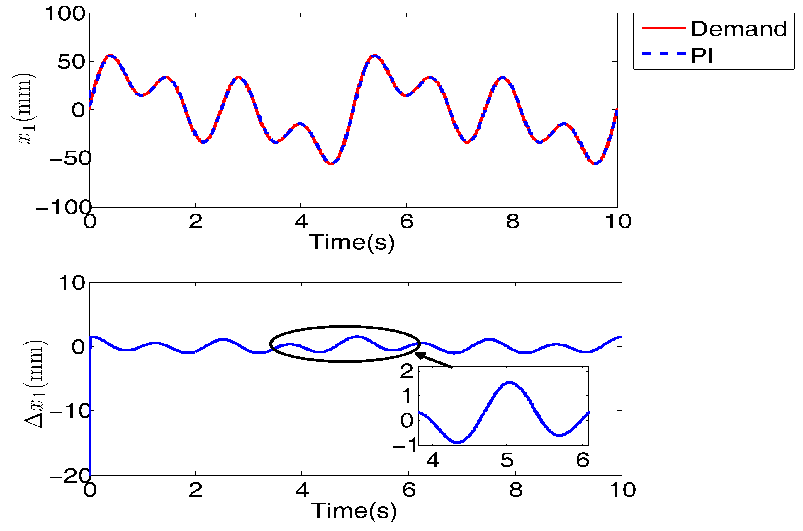
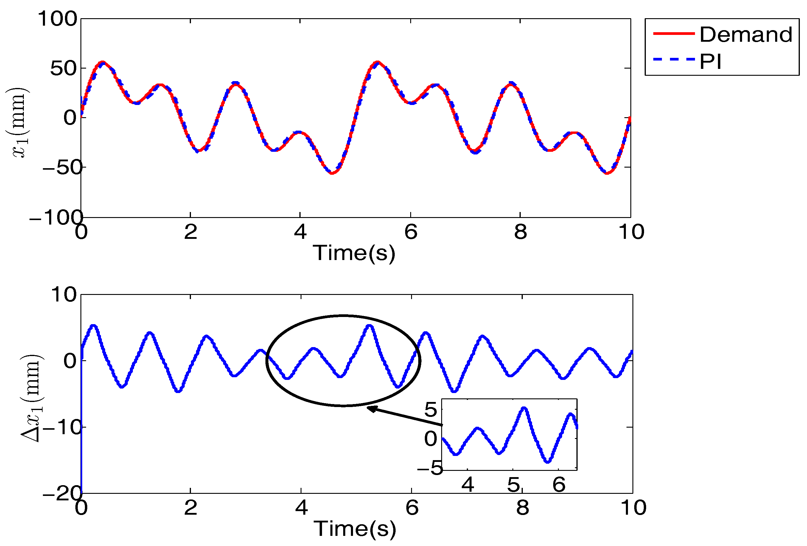
4.2. Compared Results with Uncertain Nonlinearities

To verify the dynamic response performance of the proposed prescribed performance constraint controller, the frequency of the cylinder position demands and the initial states are same to Section 4.1. The hydraulic parametric uncertainties $\Delta C_d$, $\Delta {\beta }_e$, $\Delta K$, $\Delta b$, $\Delta \rho$, $\Delta C_{tl}$ are all injected in the EHS model (2). Furthermore, the external load are assumed to be $F_L\left(t\right)=F_{L\max }\sin \left(2\pi t\right)$. The comparison results of two controllers are shown in Figure 7, Figure 8, Figure 9 and Figure 10. When the total uncertain nonlinearities ${\Delta }_2$ and ${\Delta }_3$ are injected in EHS, the prescribed performance constraint controller has the steady tracking error $\Delta x_1=2$ mm both in low and high frequency demand. However, the position tracking error of PI controller is $\Delta x_1=5$ mm. These results indicate the prescribed performance constraint controller has higher dynamic response performance than the PI controller under the hydraulic parametric uncertainties and the external load disturbance.

5. Conclusions

In this study, a prescribed performance constraint controller is proposed for electro-hydraulic system to improve the output position accuracy of EHS. Firstly, the EHS model is constructed as a state-space strict-feedback model with uncertain nonlinearities. Secondly, according to the required boundary of the tracking position error, the technique of prescribed performance constraint is used to design the time-varying error boundary to not only regulate the large initial error in satisfactory time but also consider the control capability of EHS. Furthermore, the dynamic surface is adopted to replace the repeatedly calculated differentiations of the virtual control variables in backstepping design. The comparative results with the PI controller verify that the proposed controller has better performance than PI controller.

References

1. Fales, R.; Kelkar, A. Robust control design for a wheel loader using H and feedback linearization based methods. ISA Trans. 2009, 48, 313–320. [Google Scholar] [CrossRef] [PubMed]
2. Zhao, J.; Wang, J.; Wang, S. Fractional order control to the electrohydraulic system in insulator fatigue test device. Mechatronics 2013, 23, 828–839. [Google Scholar] [CrossRef]
3. Yao, J.; Jiao, Z.; Shang, Y.; Huang, C. Adaptive nonlinear optimal compensation control for electro-hydraulic load simulator. China J. Aeronaut. 2010, 23, 720–733. [Google Scholar]
4. Yang, Y.; Ma, L.; Huang, D. Development and repetitive learning control of lower limb exoskeleton driven by electro-hydraulic actuators. IEEE Trans. Ind. Electron. 2017, 64, 4169–4178. [Google Scholar] [CrossRef]
5. Merritt, H. Hydraulic Control Systems; John Wiley & Sons: New York, NY, USA, 1967. [Google Scholar]
6. Shen, G.; Zhu, Z.; Zhao, J.; Zhu, W.; Tang, Y.; Li, X. Real-time tracking control of electro-hydraulic force servo systems using offline feedback control and adaptive control. ISA Trans. 2017, 67, 356–370. [Google Scholar] [CrossRef] [PubMed]
7. Guo, Q.; Yin, J.; Yu, T.; Jiang, D. Saturated adaptive control of an electrohydraulic actuator with parametric uncertainty and load disturbance. IEEE Trans. Ind. Electron. 2017, 64, 7930–7941. [Google Scholar] [CrossRef]
8. Shi, Y.; Wang, Y.; Cai, M.; Zhang, B.; Zhu, J. Study on the aviation oxygen supply system based on a mechanical ventilation model. Chin. J. Aeronaut. 2017. [Google Scholar] [CrossRef]
9. Shi, Y.; Zhang, B.; Cai, M.; Zhang, D. Numerical Simulation of volume-controlled mechanical ventilated respiratory system with two different lungs. Int. J. Numer. Methods Biomed. Eng. 2016, 33, 2852. [Google Scholar] [CrossRef] [PubMed]
10. Niu, J.; Shi, Y.; Cai, M.; Cao, Z.; Wang, D.; Zhang, Z.; Zhang, D.X. Detection of sputum by interpreting the time-frequency distribution of respiratory sound signal using image processing techniques. Bioinformatics 2017. [Google Scholar] [CrossRef] [PubMed]
11. Ren, S.; Shi, Y.; Cai, M.; Xu, W. Influence of secretion on airflow dynamics of mechanical ventilated respiratory system. IEEE/ACM Trans. Comput. Biol. Bioinform. 2017. [Google Scholar] [CrossRef] [PubMed]
12. Niu, J.; Shi, Y.; Cao, Z.; Cai, M.; Wei, C.; Jian, Z.; Xu, W. Study on air flow dynamic characteristic of mechanical ventilation of a lung simulator. Sci. China Technol. Sci. 2017, 45, 1–8. [Google Scholar] [CrossRef]
13. Ren, S.; Cai, M.; Shi, Y.; Xu, W.; Zhang, X.D. Influence of Bronchial Diameter Change on the airflow dynamics Based on a Pressure-controlled Ventilation System. Int. J. Numer. Methods Biomed. Eng. 2017. [Google Scholar] [CrossRef] [PubMed]
14. Shi, Y.; Zhang, B.; Cai, M.; Xu, W. Coupling Effect of Double Lungs on a VCV Ventilator with Automatic Secretion Clearance Function. IEEE/ACM Trans. Comput. Biol. Bioinform. 2017. [Google Scholar] [CrossRef] [PubMed]
15. Shi, Y.; Wu, T.; Cai, M.; Wang, Y.; Xu, W. Energy conversion characteristics of a hydropneumatic transformer in a sustainable-energy vehicle. Appl. Energy 2016, 171, 77–85. [Google Scholar] [CrossRef]
16. Shi, Y.; Wang, Y.; Liang, H.; Cai, M. Power characteristics of a new kind of air-powered vehicle. Int. J. Energy Res. 2016, 40, 1112–1121. [Google Scholar] [CrossRef]
17. Shi, Y.; Niu, J.; Cao, Z.; Cai, M.; Zhu, J.; Xu, W. Online estimation methodfor respiratory parameters based on a pneumatic model. IEEE/ACM Trans. Comput. Biol. Bioinform. 2016, 13, 939–946. [Google Scholar] [CrossRef] [PubMed]
18. Zhu, B.; Meng, C.; Hu, G. Robust consensus tracking of double-integrator dynamics by bounded distributed control. Int. J. Robust Nonliner Control 2016, 26, 1489–1511. [Google Scholar] [CrossRef]
19. Zhu, B.; Liu, H.H.T.; Li, Z. Robust distributed attitude synchronization of multiple three-DOF experimental helicopters. Control Eng. Pract. 2015, 36, 87–99. [Google Scholar] [CrossRef]
20. Zhang, Y.; Su, S.; Savkin, A.; Celler, B.; Nguyen, H. Multiloop integral controllability analysis for nonlinear multiple-input single-output Processes. Ind. Eng. Chem. Res. 2017, 56, 8054–8065. [Google Scholar] [CrossRef]
21. Tee, K.P.; Ge, S.S.; Tay, E.H. Barrier lyapunov functions for the control of output-constrained nonlinear systems. Automatica 2009, 45, 918–927. [Google Scholar] [CrossRef]
22. Tee, K.P.; Ren, B.; Ge, S.S. Control of nonlinear systems with time varying output constraints. Automatica 2011, 47, 2511–2516. [Google Scholar] [CrossRef]
23. He, W.; Chen, Y.; Yin, Z. Adaptive neural network control of an uncertain robot with full-state constraints. IEEE Trans. Cybern. 2016, 46, 620–629. [Google Scholar] [CrossRef] [PubMed]
24. He, W.; David, A.O.; Yin, Z.; Sun, C. Neural network control of a robotic manipulator with input deadzone and output constraint. IEEE Trans. Syst. Man Cybern. A Syst. 2016, 46, 759–770. [Google Scholar] [CrossRef]
25. He, W.; Huang, H.; Ge, S.S. Adaptive neural network control of a robotic manipulator with time-varying output constraints. IEEE Trans. Cybern. 2017, 47, 3136–3147. [Google Scholar] [CrossRef] [PubMed]
26. He, W.; Dong, Y. Adaptive fuzzy neural network control for a constrained robot using impedance learning. IEEE Trans. Neural Netw. Learn. Syst. 2017. [Google Scholar] [CrossRef] [PubMed]
27. Ren, B.; Ge, S.S.; Tee, K.P.; Lee, T.H. Adaptive neural control for output feedback nonlinear systems using a barrier lyapunov function. IEEE Trans. Neural Netw. 2010, 21, 1339–1345. [Google Scholar] [PubMed]
28. Won, D.; Kim, W.; Shin, D.; Chung, C.C. High-gain disturbance observer-based backstepping control with output tracking error constraint for electro-hydraulic systems. IEEE Trans. Control Syst. Technol. 2015, 23, 787–795. [Google Scholar] [CrossRef]
29. Qiu, Y.; Liang, X.; Dai, Z. Backstepping dynamic surface control for an anti-skid braking system. Control Eng. Pract. 2015, 42, 140–152. [Google Scholar] [CrossRef]
30. Guo, Q.; Zhang, Y.; Celler, B.G.; Su, S.W. State-constrained control of single-rod electrohydraulic actuator with parametric uncertainty and load disturbance. IEEE Trans. Control Syst. Technol. 2017. [Google Scholar] [CrossRef]
31. Bechlioulis, C.P.; Rovithakis, G.A. Adaptive control with guaranteed transient and steady state tracking error bounds for strict feedback systems. Automatica 2015, 45, 532–538. [Google Scholar] [CrossRef]
32. Zhang, Z.; Duan, G.; Hou, M. Robust adaptive dynamic surface control of uncertain non-linear systems with output constraints. IET Control Theory Appl. 2017, 11, 110–121. [Google Scholar] [CrossRef]
33. Zhang, Z.; Duan, G.; Hou, M. Longitudinal attitude control of a hypersonic vehicle with angle of attack constraints. In Proceedings of the 10th Asian Control Conference, Kota Kinabalu, Malaysia, 31 May–3 June 2015. [Google Scholar]
34. Swaroop, D.; Hedrick, J.; Yip, P.; Gerdes, J. Dynamic surface control for a class of nonlinear systems. IEEE Trans. Autom. Control 2000, 45, 1893–1899. [Google Scholar] [CrossRef]
35. Wang, D.; Huang, J. Neural network-based adaptive dynamic surface control for a class of uncertain nonlinear systems in strict-feedback form. IEEE Trans. Neural Netw. 2005, 16, 195–202. [Google Scholar] [CrossRef] [PubMed]
36. Hou, M.; Duan, G. Robust adaptive dynamic surface control of uncertain nonlinear systems. Int. J. Control Autom. Syst. 2011, 9, 161–168. [Google Scholar] [CrossRef]
37. Kim, W.; Shin, D.; Won, D.; Chung, C.C. Disturbance-observerbased position tracking controller in the presence of biased sinusoidal disturbance for electrohydraulic actuators. IEEE Trans. Control Syst. Technol. 2013, 21, 2290–2298. [Google Scholar] [CrossRef]
38. Yao, J.; Jiao, Z.; Ma, D. High-accuracy tracking control of hydraulic rotary actuators with modeling uncertainties. IEEE/ASME Trans. Mechatron. 2014, 19, 633–641. [Google Scholar] [CrossRef]
39. Guo, Q.; Zhang, Y.; Celler, B.G.; Su, S.W. Backstepping control of electro-hydraulic system based on extended-state-observer with plant dynamics largely unknown. IEEE Trans. Ind. Electron. 2016, 63, 6909–6920. [Google Scholar] [CrossRef]
40. Yao, J.; Jiao, Z.; Ma, D. A practical nonlinear adaptive control of hydraulic servomechanisms with periodic-like disturbances. IEEE/ASME Trans. Mechatron. 2015, 20, 2752–2760. [Google Scholar] [CrossRef]
41. Guo, Q.; Sun, P.; Yin, J.; Yu, T.; Jiang, D. Parametric adaptive estimation and backstepping control of electro-hydraulic actuator with decayed memory. ISA Trans. 2016, 62, 202–214. [Google Scholar] [CrossRef] [PubMed]
42. Krstic, M.; Kanellakopoulos, I.; Kokotovic, P.V. Nonlinear and Adaptive Control Design; John Wiley & Sons: New York, NY, USA, 1995. [Google Scholar]
Figure 1. The EHS control mechanism.
Applsci 08 00076 g001
Figure 2. Block diagram of the prescribed performance constraint controller.
Applsci 08 00076 g002
Figure 3. The cylinder position responses x 1 by PI controller with Δ 2 = Δ 3 = 0 , the demand y d = 25 ( sin ( 0.8 π t ) + sin ( 0.4 π t ) + sin ( 0.2 π t ) ) mm.
Applsci 08 00076 g003
Figure 4. The cylinder position responses x 1 by prescribed performance constraint controller with Δ 2 = Δ 3 = 0 , the demand y d = 25 ( sin ( 0.8 π t ) + sin ( 0.4 π t ) + sin ( 0.2 π t ) ) .
Applsci 08 00076 g004
Figure 5. The cylinder position responses x 1 by PI controller with Δ 2 = Δ 3 = 0 , the demand y d = 25 ( sin ( 1.6 π t ) + sin ( 0.8 π t ) + sin ( 0.4 π t ) ) .
Applsci 08 00076 g005
Figure 6. The cylinder position responses x 1 by prescribed performance constraint controller with Δ 2 = Δ 3 = 0 , the demand y d = 25 ( sin ( 1.6 π t ) + sin ( 0.8 π t ) + sin ( 0.4 π t ) ) .
Applsci 08 00076 g006
Figure 7. The cylinder position responses x 1 by PI controller with hydraulic parametric uncertainties and the external load, the demand y d = 25 ( sin ( 0.8 π t ) + sin ( 0.4 π t ) + sin ( 0.2 π t ) ) mm.
Applsci 08 00076 g007
Figure 8. The cylinder position responses x 1 by prescribed performance constraint controller with hydraulic parametric uncertainties and the external load, the demand y d = 25 ( sin ( 0.8 π t ) + sin ( 0.4 π t ) + sin ( 0.2 π t ) ) mm.
Applsci 08 00076 g008
Figure 9. The cylinder position responses x 1 by PI controller with hydraulic parametric uncertainties and the external load, the demand y d = 25 ( sin ( 1.6 π t ) + sin ( 0.8 π t ) + sin ( 0.4 π t ) ) mm.
Applsci 08 00076 g009
Figure 10. The cylinder position responses x 1 by prescribed performance constraint controller with hydraulic parametric uncertainties and the external load, the demand y d = 25 ( sin ( 1.6 π t ) + sin ( 0.8 π t ) + sin ( 0.4 π t ) ) mm.
Applsci 08 00076 g010