Article

A Fuzzy State-of-Charge Estimation Algorithm Combining Ampere-Hour and an Extended Kalman Filter for Li-Ion Batteries Based on Multi-Model Global Identification

College of Mechanical Engineering, University of Shanghai for Science and Technology, Shanghai 200093, China
*
Authors to whom correspondence should be addressed.
Appl. Sci. 2018, 8(11), 2028; https://doi.org/10.3390/app8112028
Submission received: 25 September 2018 / Revised: 17 October 2018 / Accepted: 21 October 2018 / Published: 23 October 2018
(This article belongs to the Special Issue Electric Vehicle Charging)

Abstract

:

Featured Application

The proposed fuzzy state-of-charge (SOC) estimation algorithm, combining ampere-hour and an extended Kalman filter, can be utilized as an effective SOC estimation algorithm, with high accuracy and robustness, in the whole SOC area. The proposed algorithm helps to overcome the shortcomings of commonly used SOC estimation methods, which are based on ideal conditions of no or very small model and sensor errors, and thus encounter problems in practical applications where such errors are significant, especially due to the ageing of the battery or its subjection to adverse temperatures.

Abstract

The popular and widely reported lithium-ion battery model is the equivalent circuit model (ECM). The suitable ECM structure and matched model parameters are equally important for the state-of-charge (SOC) estimation algorithm. This paper focuses on high-accuracy models and the estimation algorithm with high robustness and accuracy in practical application. Firstly, five ECMs and five parameter identification approaches are compared under the New European Driving Cycle (NEDC) working condition in the whole SOC area, and the most appropriate model structure and its parameters are determined to improve model accuracy. Based on this, a multi-model and multi-algorithm (MM-MA) method, considering the SOC distribution area, is proposed. The experimental results show that this method can effectively improve the model accuracy. Secondly, a fuzzy fusion SOC estimation algorithm, based on the extended Kalman filter (EKF) and ampere-hour counting (AH) method, is proposed. The fuzzy fusion algorithm takes advantage of the advantages of EKF, and AH avoids the weaknesses. Six case studies show that the SOC estimation result can hold the satisfactory accuracy even when large sensor and model errors exist.

1. Introduction

Due to increasing concerns about global warming, greenhouse gas emissions, and the depletion of fossil fuels, electric vehicles (EVs) have gained massive popularity due to their performances and efficiencies in recent decades [1,2,3]. Lithium-ion batteries (LIBs) are widely used in EVs for their high-energy density, long service life, and environmental friendliness [4,5,6]. In actual practice, LIBs need to be well monitored, diagnosed, and controlled by the battery management system (BMS). The accurate state estimation of a battery is one of the most fundamental functions of the BMS. The states of the battery include state-of-charge (SOC), state-of-health (SOH), and state-of-function (SOF) etc. [7,8]. Among these states, SOC in BMS is considered as one of the critical and important factors [9,10], which have been researched in recent decades. Accurate battery state estimation can contribute to reasonable management of batteries to fully exploit them and prolong their lifespan. However, the battery states are non-measurable variables, which can only be indirectly estimated via measurable external characteristic parameters (e.g., voltage, current, and temperature). Owing to the high nonlinearity of the battery system itself, accurate estimation of the battery state is fairly difficult.

1.1. Literature Review

With the development of BMS, a large number of SOC estimation methods have been proposed and each one has its own merits and limitations [4,11]. The commonly used methods in the literature can be listed as follows [12,13]: (1) ampere-hour (AH) counting method; (2) open-circuit voltage (OCV) method; (3) model-based method; and (4) neural-network model method. Among these methods, the AH method is most extensively used owing to its ease of implementation. However, it suffers from the drawbacks of accumulated errors. Another classic method is the model-based method, where the Kalman filter (KF) algorithm is generally used [1,14]. Due to its high applicability and accuracy, various forms of the KF algorithm, such as the linear KF (LKF), single KF (SKF), unscented KF (UKF), sigma point KF (SPKF), and extended KF (EKF), have been intensively investigated in recent years [15].
In the practical application of SOC estimation, many factors affect its accuracy. These factors mainly include model and sensor errors [16]. The sensor errors include the voltage and current sensor errors in the BMS, while the model errors include the battery capacity, coulombic efficiency, and ECM errors. The model errors increase with LIB ageing and exposure to adverse temperatures. These errors increase the SOC estimation error. Therefore, the influence of these factors on SOC must be considered to improve the robustness of the SOC estimation algorithm in the actual BMS.
The model-based estimator is widely used in the existing SOC estimation. Therefore, an accurate battery model is the prerequisite for precise SOC estimation. The equivalent circuit model (ECM) has the advantages of simple structure, small number of identification parameters, and high accuracy, which have made it become the most popular battery model for existing BMSs [17]. At present, the ECMs mainly include the resistance-capacitance model with different orders (nRC, n = 0, 1, 2, etc.), GNL (general nonlinear) model, and PNGV (the Partnership for a New Generation of Vehicle) model, etc., and the most commonly used model is nRC [18,19]. The characteristics and accuracy of the ECM are affected by the structure and parameters of the model. Therefore, a reasonable model structure and matched model parameters are indispensable for the accurate SOC estimation. It is inappropriate to apply simple parameter identification algorithms to complex models nor complex parameter identification algorithms to simple models. In other words, high model accuracy can only be achieved by using a suitable battery model and matched model parameters at the same time. In this regard, the parameter identification approach and the model structure are equally important. To the best of our knowledge, the parameter identification of ECMs is an optimization problem, and there are many identification algorithms to determine the battery model parameters in the literature, such as the genetic algorithm [20], the particle swarm optimization algorithm [21], and the least-squares method [22]. Previous studies on LIB models have not paid much attention to whether a parameter identification approach is suitable for a certain model. In this paper, we investigated the accuracy of various models in various identification algorithms to determine the most appropriate model structure and parameter identification algorithm for the whole SOC area.

1.2. Main Contributions

In order to improve the accuracy and robustness of the SOC estimation algorithm, based on ECMs in the whole SOC area, this paper aims to make three contributions:
(1)
By comparing and analyzing nine models and five commonly used parameter identification algorithms, the most suitable ECM and parameter identification algorithm are decided.
(2)
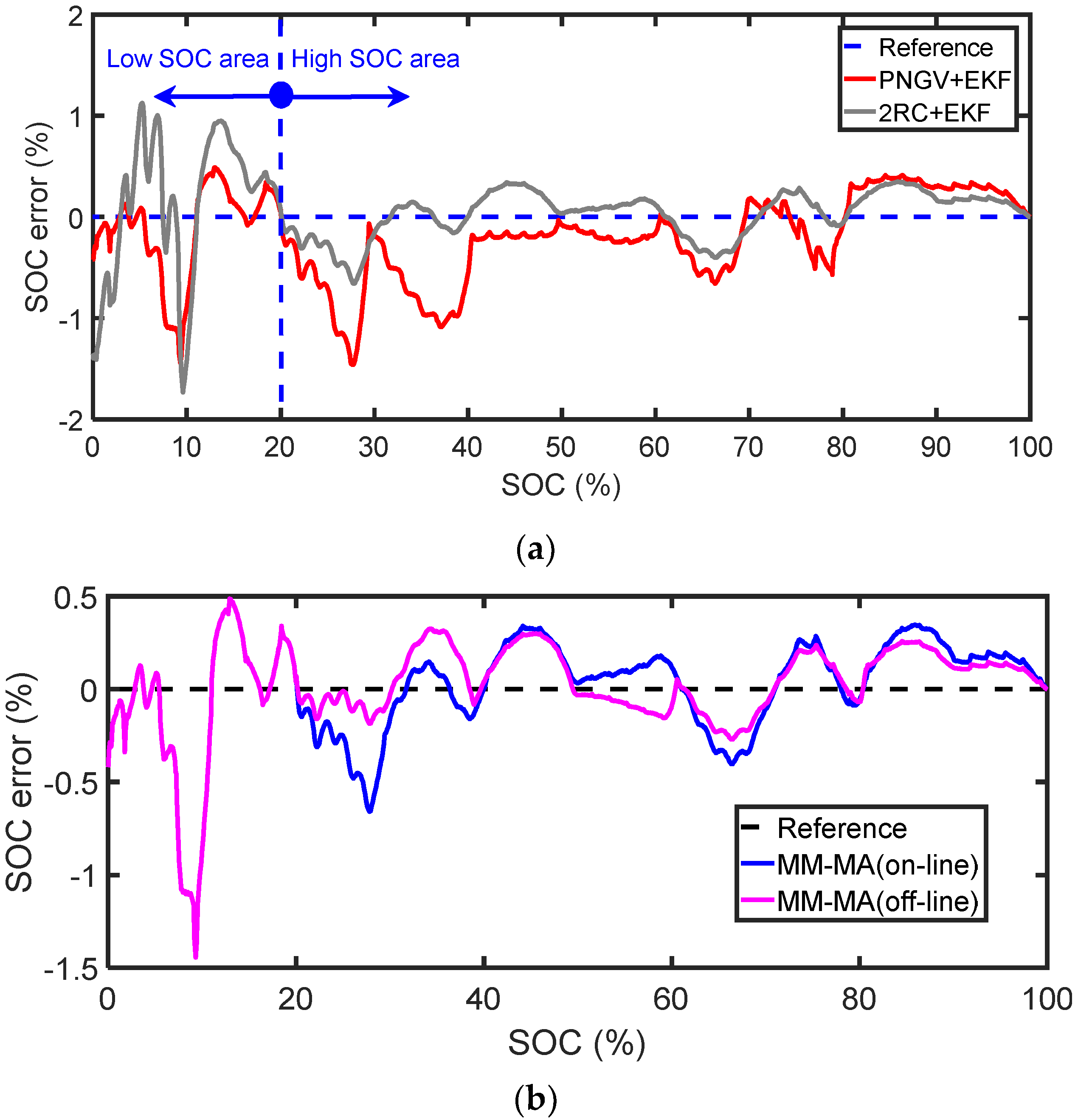
The whole SOC area is divided into the high SOC area and low SOC area. Different ECMs and parameter identification algorithms are adopted considering SOC distribution. Based on this, a multi-model and multi-algorithm method is developed to fit the battery model. Experimental results show that the proposed composite model has higher model accuracy compared with a single model.
(3)
According to the error characteristics of EKF and AH, a fuzzy fusion SOC estimation algorithm, combining AH and EKF in the whole SOC area, is proposed, and the accuracy and robustness of the proposed algorithm are verified by six cases.

1.3. Organization of the Paper

The remainder of this paper is organized as follows. Section 2 describes the experimental equipment and the curves of current and voltage variation under the New European Driving Cycle (NEDC) working condition in the whole SOC area. Section 3 introduces five ECMs and five parameter identification approaches in five categories. The most suitable model and parameter identification algorithm are selected through comparative study. In Section 4, a fuzzy fusion algorithm, based on the EKF and AH, is proposed. In Section 5, the results of SOC estimation are analyzed and discussed. Finally, Section 6 states the conclusions.

2. Experiments

A commercial prismatic pouch lithium-ion cell was tested in this study. The cathode material of the cell was LiNixCoyMn1−x−yO2 (NMC). The basic parameters of the cell are listed in Table 1. The experiments were conducted in a test bench made by DIGATRON, which had a current range of −100 to +100 A and a voltage range of 0 to 20 V. The tested cell was put into a temperature chamber to keep the ambient temperature. The temperature chamber was made by Dongguan Bell Company and the type was TEMI580.
Firstly, the capacity test was designed to find the standard capacity of the test cell (Cell#1). The capacity test process was as follows: Cell#1 was placed in the temperature chamber at 25 °C for 3 h. Then, Cell#1 was discharged at a constant discharge current (1/3 C) to 2.5 V. After waiting for 1 h, Cell#1 was fully charged using the constant current-constant voltage method. This process was repeated three times, and the average value of the test capacity was taken as the standard capacity of the test cell. Secondly, the hybrid pulse power characterization (HPPC) test was carried out to find the open circuit voltage (OCV). The test steps can be found in References. [2,6], specific steps are not listed here for brevity.
Finally, Cell#1 was fully charged at 1/3 C. Then, the discharge process was performed under the NEDC cycles. PC software (BTS-600) was used to record the voltage and current of the cell in real time. Figure 1b,c show these test data, which were used for the model parameter identification and the SOC estimation.

3. Model and Parameter Identification

3.1. Equivalent Circuit Models

In this study, we chose the popular and widely reported nRC, nRCH, and PNGV models as battery models. The schematics of the three models is shown in Figure 2. In these models, U O C V denotes battery voltage source, U L is the terminal voltage, R 0 denotes equivalent ohmic resistance, and R i and C i denote diffusion resistance and diffusion capacitance, respectively. u h , k is the hysteresis voltage, k p is a decaying factor, and M is the maximum amount of hysteresis voltage. C b in the PNGV model is an equivalent capacitance, which describes the changes in the OCV caused by time accumulation. The equations of ECMs are presented in Table 2.

3.2. Optimization Variables and the Objective Function for ECMs

In the nRC, nRCH, and PNGV, the model parameters should be identified optimally. The model parameters to be determined by optimization algorithm can be expressed as:
V j { [ R 0 + R 0 τ 1 R 1 1 s t   RC τ 2 R 2 2 n d   RC τ n R n n - t h   RC   ] ( if   the   model   is   nRC ) [ R 0 + R 0 τ 1 R 1 1 s t   RC τ 2 R 2 2 n d   RC τ n R n n - t h   RC k p M hysteresis ] ( if   the   model   is   nHRC ) [ R 0 + R 0 τ 1 R 1 C b ] ( if   the   model   is   PNGV )
where R 0 + and R 0 represent the ohmic resistance of charging and discharging, respectively.
From (1), it was seen that the number of parameters to be identified increased with the order of ECM. For the 4RC model, the number of parameters to be identified can reach up to 10. In this study, the root-mean-square error (RMSE) between the model terminal voltage and the measured terminal voltage was used to evaluate the fitness of model parameters. Correspondingly, the fitness function can be expressed as:
M E M S E ( θ ) = 1 n k = 1 n ( u i , k ( θ ) u ^ i , k ( θ ) ) 2  
where M R M S E represents the RMSE of the ECM, u i , k represents the voltage of ECM, and u ^ i , k represents the test voltage.

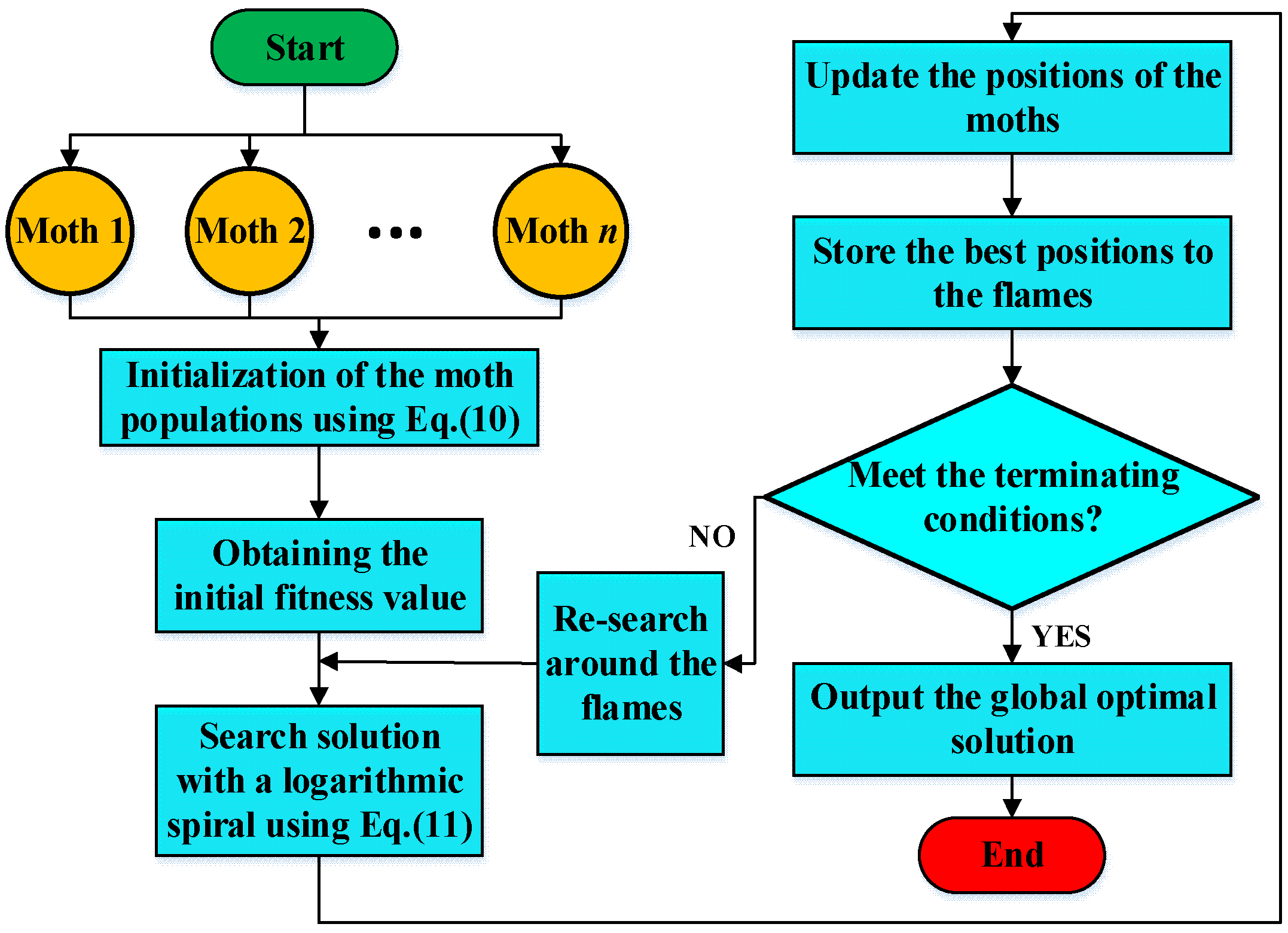
3.3. Moth-Flame Optimization Algorithm

The moth-flame optimization (MFO) algorithm is a nature-inspired optimization proposed by Seyedali Mirjalili in 2015 [23]. Many examples show that the MFO algorithm has the advantages of strong convergence, fast convergence, and wide application, and it is suitable for solving the problem of high dimensional optimization. In the MFO algorithm, it was assumed that the candidate solutions were moths and the problem’s variables were the position of moths in the space. Other key components in the MFO were flames. The set of moths and flames are represented in the following matrices:
M = [ M 1 , 1 M 1 , 2 M 1 , d M 2 , 1 M 2 , 2 M 2 , d M n , 1 M n , 2 M n , d ] ,   F = [ F 1 , 1 F 1 , 2 F 1 , d F 2 , 1 F 2 , 2 F 2 , d F n , 1 F n , 2 F n , d ]  
where n is the number of moths and flames, and d is the number of variables.
For all the moths and flames, we assumed that there were two arrays for storing the corresponding fitness values, as follows:
O M = [ O M 1 O M 2 O M n ] ,   O F = [ O F 1 O F 2 O F n ]  
In the MFO, a random initial solution to calculate the objective function values can be described as follows:
M i , j = ( u b i l b i ) r a n d (   ) + l b i  
where u b i and l b i are the upper and lower bounds of the variables. r a n d (   ) is a random function.
The position of each moth was updated with respect to a flame using the following equation:
M i = S ( M i , F j ) = | F j - M i | e b t cos ( 2 t ) + F j  
where b is a constant, and t is a random number in [−1, 1]. S is the spiral function.
Figure 3 shows the flow chart of the MFO algorithm. The terminating conditions included the maximum iteration times and the solution accuracy to meet the setup requirements.
In order to verify the performance of the MFO algorithm and select the most suitable identification algorithm, five well-known algorithms in five categories, as shown in Table 3, were chosen to identify the parameters of the ECMs shown in Table 2. For concise description, the other algorithms are not described here.
Moreover, the whole SOC (0–100%) was divided into 10 subarea, and the parameters in each subarea were identified by the above optimization algorithms, respectively. Therefore, 10 groups of model parameters, which vary with SOC, were obtained as the model parameters of ECM.

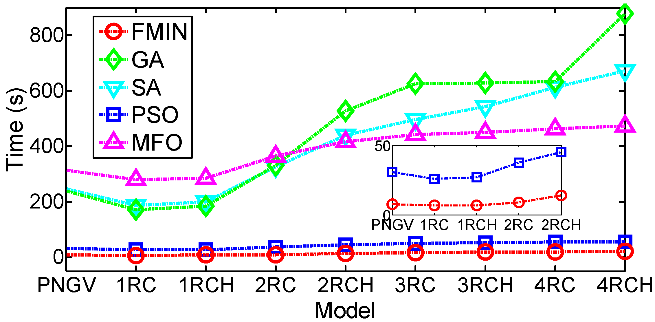
3.4. Comparative Study of Optimization Methods

In this study, the above five optimization methods were used to identify the nine ECMs, respectively, then the appropriate models and algorithms were selected by comparing the identification accuracy and time cost.
Figure 4a shows the RMSE of model error in the entire SOC area. It can be seen that the PNGV had a great accuracy advantage. For the nRC model, the model accuracy of the MFO increased with the increase of n, and the accuracy of the other optimization algorithms did not increase or even decrease when the order was greater than the second. Moreover, MFO had an obvious accuracy advantage for the high-order RC model. The model error distribution in the low SOC area (0–20%) is shown in Figure 4b, indicated that the PNGV model had obvious advantages in the low SOC area, and the FMIN, PSO, and MFO had almost the same identification accuracy. The error distribution comparison between the PNGV model and the 2RC model in the low SOC area is shown in Figure 5. It is clear that the PNGV model had a good accuracy in the low SOC area. The error distribution in the high SOC area (20–100%) is shown in Figure 4c. It can be seen that the second- and higher-order RC models had high accuracy using PSO and MFO, and the accuracy of MFO was slightly higher. The identification time of each identification algorithm is shown in Figure 6. It can be seen that the FMIN had the shortest identification time, and PSO had the second shortest identification time (approximately one-sixth of the time taken by the other algorithms). Therefore, these two algorithms are suitable for on-line identification.
Based on the above analysis, we could see that the PNGV model was the best choice, and the matched identification algorithm was FMIN in the low SOC area. In the high SOC area, if it was on-line identification, 2RC plus PSO was the best choice for the balance between accuracy and time cost. If it was off-line identification, 4RC plus MFO was the best choice for the highest accuracy.

3.5. Multi-Model and Multi-Algorithm Combination

Based on the above analysis, a multi-model and multi-algorithm combination (MM-MA) method, considering SOC distribution, was developed to improve the global accuracy of the ECM. As shown in Figure 7, the whole SOC area was divided into low SOC area and high SOC area, and different ECMs and optimization algorithms were used in different SOC areas. In the SOC estimation, different ECMs and corresponding model parameters were selected.
Figure 8 shows the identification results of the MM-MA method, which indicated that this method had obvious advantages compared with 2RC, especially in the low SOC area. Moreover, the accuracy of off-line identification was higher than that of on-line identification. It was shown that the MM-MA method could effectively improve the accuracy of the model, and could lay the foundation for accurate SOC estimation.

4. SOC Estimation Method

4.1. EKF Method

For the second-order RC model, the state variables (x) can be written as:
x = [ SOC E K F , U 1 , U 2 ] T  
From Table 2, the following expressions can be obtained:
f ( x k , u k ) = [ 1 0 0 0 exp ( Δ t / τ 1 ) 0 0 0 exp ( Δ t / τ 2 ) ] [ SOC E K F , k U 1 , k U 2 , k ]       + [ η Δ t / C n R 1 ( 1 exp ( Δ t / τ 1 ) ) R 2 ( 1 exp ( Δ t / τ 2 ) ) ] I k
g ( x k , u k ) = U o c ( SOC E K F , k ) I k R 0 U 1 , k U 2 , k  
where Δ t is the sample period.
The form of the state-space expression of the fourth-order RC and PNGV models was similar to (7)–(9), which is not given here for brevity. According to the reference [27], the standard EKF equations for the battery system are listed in Algorithm 1.
Many studies have confirmed that the EKF method produces a good convergence and satisfactory estimation accuracy for small model and sensor errors [14,16,28,29,30]. However, in actual EV operation, the ECM model error increased with battery ageing, temperature, and other adverse factors. Moreover, the sensor measurement error existed objectively, and the random error of the statistical characteristics of the noise is unknown. Under these circumstances, the accuracy of the SOC estimation error determined by the EKF method would decrease. Therefore, model and sensor errors must be considered for designing SOC estimation algorithm to improve the robustness.
Algorithm 1. Summary of the extended Kalman filter (EKF) method for SOC estimation.
The nonlinear state-space model:
{ x k + 1 = f ( x k , u k ) + w k y k = f ( x k , u k ) + v k
where the first equation is the state equation, the second one is the output equation. f ( x k , u k ) is a state transition function and g ( x k , u k ) is a measurement function; w k and v k are independent zero-mean white Gaussian stochastic processes with covariance matrices w and v respectively.
Step 1. Initialization.
For k = 0 , set
x ^ 0 + = E [ x ^ 0 ] ,   x , 0 + = E [ ( x 0 x ^ 0 + ) ( x 0 x ^ 0 + ) T ] .
Step 2. Computation.
For k = 1 , 2 , , compute:
(a)
Time update:
x ^ k = f ( x ^ k 1 + , u k 1 ) + w k 1 ; x , k = A k 1 x , k 1 + A k 1 T + w .
(b)
Measurement update:
Error innovation: e k = y k y ^ k = y k g ( x ^ k , u k ) .
Kalman gain matrix: L k x = x , k ( C k x ) T [ C k x Χ k x x , k ( C k x ) T + v ] 1
Measurement update: x ^ k + = x ^ k + L k x [ y k y ^ k ]
Error covariance measurement update: x , k + = ( I L k x C k x ) x , k
where A k = f ( x k , u k ) x | x = x ^ k + , C k = g ( x k , u k ) x | x = x ^ k

4.2. Ampere-Hour Counting Method

The AH method can be expressed as follows [31]:
SOC A H ( t ) = SOC ( t 0 ) + η c t 0 t i ( ξ ) d ξ C N  
where SOC A H ( t ) is the SOC value at time t , SOC ( t 0 ) is the SOC value at the initial time t 0 , C N is the nominal capacity, i ( ξ ) denotes the current at time ξ (positive for charging and negative for discharging), and η c denotes the columbic efficiency.
Although the AH method is very simple and quite useful, it is an open-loop prediction method, thus it suffers from accumulated errors caused by initial SOC value errors, and noise and measurement errors. Moreover, the battery capacity might change in applications, which can lead to SOC error.

4.3. Fuzzy Fusion Algorithm

From the above analysis, we can see that the EKF method had high accuracy, but it was easy to be influenced by ECM model parameters and voltage sensor errors. The AH method had relatively low accuracy, but the estimation results were relatively stable because relatively few parameters were affected. Based on the characteristics of the above two algorithms, a fuzzy fusion method, combining AH and EKF, was developed to calculate SOC in this paper. In our algorithm, the SOC was estimated by the AH and EKF methods, respectively. Then, the SOC increments were calculated using the following equations:
Δ SOC A H ( k ) = SOC A H ( k ) SOC A H ( k 1 )  
Δ SOC E K F ( k ) = SOC E K F ( k ) SOC E K F ( k 1 )  
where Δ SOC A H ( k ) and Δ SOC E K F ( k ) are the SOC increments for the AH and EKF methods, respectively.
Then, EKF and AH methods can be fused through the following incremental form:
S O C f ( k ) = S O C f ( k 1 ) + k F L C Δ S O C E K F ( k ) + ( 1 k F L C ) Δ S O C A H ( k )  
where S O C f ( k ) is the SOC value determined by the fusion algorithm, k F L C is ratio coefficient ( 0 k F L C 1 ) .
The most critical step of the fusion algorithm is the determination of the more credible SOC increments between Δ SOC A H ( k ) and Δ SOC E K F ( k ) . In other words, the key to SOC estimation in (13) is to select suitable k F L C based on the relationship between Δ SOC A H ( k ) and Δ SOC E K F ( k ) . We assume that the incremental ratio of SOC estimated by the two methods at time k is Δ K S O C ( k ) , and it can be expressed as follows:
Δ K S O C ( k ) = | Δ SOC E K F ( k ) | | Δ SOC A H ( k ) |  
In this study, the fuzzy logic control was used to determine the appropriate k F L C based on Δ K S O C ( k ) . The range of Δ K S O C ( k ) was set as 0 to 3 in this paper. In the fuzzy logic control, the input and output were divided into fuzzy subsections and expressed by a linguistic variable.
As shown in Figure 9, we chose Δ K S O C ( k ) and its derivative Δ K S O C ( k ) as input variables and k F L C as output variables. The fuzzy variable of Δ K S O C ( k ) was divided into very large (VL), large (L), medium (M), small (S), and very small (VS). Δ K S O C ( k ) was divided into positive (P), zero (Z), and negative (N). The fuzzy variable of output with respect to k F L C was divided into VL, L, M, S, and VS. The triangular fuzzy membership function was chosen in this paper because the triangular membership function has the characteristics of simplified calculation and good control performance. The membership function of FLC is shown in Figure 10.
Considering the sensor and model errors, the AH method may not be very accurate, but it had higher reliability increments due to less affected parameters. The EKF method had good accuracy, but it may not be stable. Therefore, we can choose the SOC increment with high reliability and accuracy based on the relative relationship between Δ SOC A H ( k ) and Δ SOC E K F ( k ) to calculate SOC according to the value of Δ K S O C ( k ) . Based on the above characteristics, the following rules were proposed for determining the higher credibility SOC increment between the two methods: (1) If Δ K S O C ( k ) 1 , then Δ SOC E K F ( k ) is considered to be more credible (large k F L C should be chosen); (2) if Δ K S O C ( k ) > 1 , then Δ SOC A H ( k ) is considered to be more credible (small k F L C should be chosen); and (3) if Δ K S O C ( k ) < 0 , it means that Δ K S O C ( k ) has a decreasing trend, otherwise there is an increasing trend. Therefore, the fuzzy rule of the fuzzy fusion algorithm can be expressed as follows:
  • When Δ K S O C ( k ) is relatively small and Δ K S O C ( k ) is negative, very large k F L C should be chosen to ensure that Δ SOC E K F ( k ) is more credible in the fuzzy fusion algorithm.
  • When Δ K S O C ( k ) is relatively large and Δ K S O C ( k ) is positive, very small k F L C should be chosen to ensure that Δ SOC A H ( k ) is more credible in the fuzzy fusion algorithm.
  • When Δ K S O C ( k ) is relatively large and Δ K S O C ( k ) is negative, small k F L C should be chosen.
  • When Δ K S O C ( k ) is relatively small and Δ K S O C ( k ) is positive, medium k F L C should be chosen to improve the stability of the control system.
Based on the above four rules, 15 control rules for linguistic variables were obtained, shown in Table 4. The fuzzy linguistic output is an unavailable signal for the SOC estimation system. Therefore, the defuzzification is necessary, which is the process of relating the output membership function to a value. The centroid defuzzification method was utilized in this paper, and it can be expressed as follows:
k F L C = z μ ( z ) d z μ ( z ) d z  
The proposed fuzzy fusion algorithm uses the incremental features of EKF and AH to design fuzzy characteristics, which effectively avoids the shortcomings of the two algorithms and takes advantage of their advantages.

5. Results and Discussion

5.1. Estimation Results Based on EKF

The SOC estimation error based on EKF is shown in Figure 11. It can be seen that the SOC accuracy based on the PNGV model in the low SOC area was higher than that based on the 2RC model, and that SOC estimation accuracy based on off-line identification was higher than that based on on-line identification. The results indicate that the proposed MM-MA method can improve the accuracy of the model and the SOC estimation significantly.
The reason why the accuracy of off-line identification was higher than that of on-line identification is that the more complex model and more suitable identification algorithm (4RC plus MFO) were used for off-line identification. However, greater computing burden and more identification time were needed for off-line identification, which is shown in Figure 6.

5.2. Case Studies for the Fuzzy Fusion Algorithm

To verify and evaluate the effectiveness of the proposed fuzzy fusion algorithm, six simulated cases of real LIBs, considering sensor and model errors, were set, as shown in Table 5. The fuzzy fusion algorithm was carried out based on these cases. In addition, the AH and EKF methods were applied to the same cases for comparison. In Table 5, e S O C 0 is the initial SOC error, ECM d r i f t is the ECM error, I d r i f t is the drift current of the current sensor, U d r i f t is the drift voltage of the voltage sensor, and e O C V is the SOC–OCV curve error. In this study, SOH is expressed as Equation (16), where S O H i means the SOH value in the ith cycle, Ci represents the capacity at the ith cycle, C0 represents the initial capacity. With aging of the cell, the cell capacity shows a downward trend.
S O H i = C i C 0 × 100 %  
To evaluate the performance of different SOC estimation methods, the root-mean-square errors (RMSE) of SOC were calculated as follows:
RMSE = 1 m k = 1 m ( S O C r e l ( k ) S O C E s t i m a t e d ( k ) ) 2  
where S O C r e l and S O C E s t i m a t e d denote the real and estimated values of the SOC, respectively.
Figure 12 shows the SOC estimation results for Case A. It indicated the influence of initial SOC error ( e S O C 0 ) on the AH, EKF, and fuzzy fusion algorithm (fuzzy). It was clear that e S O C 0 had no effect on the EKF method, but significantly affected the AH and the fuzzy methods. Figure 12a,c show that the fuzzy fusion algorithm had a higher estimation accuracy when the initial SOC error was more accurate ( | e S O C 0 | < 3 % ). When e S O C 0 was large, the fuzzy fusion algorithm had a larger estimation error than the other algorithms (Figure 12b). However, the initial SOC correction methods, such as the full-charge calibration method or the OCV method (e.g., with a 3 h rest for the LIBs), were used in the practical EV applications. Therefore, an accurate initial SOC could be ensured, improving the feasibility of the fuzzy fusion method for real EVs.
Moreover, Figure 12c shows that the SOC estimation accuracy based on the MM-MA method was higher than that based on the 2RC model, which validates the effectiveness of the proposed MM-MA method to improve the SOC estimation accuracy by improving the model accuracy.
Figure 13 shows the SOC estimation results for Case B, including the relationship between the model error and the SOC error, for the three methods. Figure 13a shows that the SOC accuracy of the fuzzy fusion algorithm exceeded that of the EKF when the model error was large. As shown in Figure 13b, the SOC accuracy of the fuzzy fusion algorithm was lower than the EKF when the model error was very small. Figure 13c shows the relationship between the SOC errors based on three algorithms and model errors of ECM. It was obvious that the accuracy of the fuzzy fusion algorithm was higher than that of both the EKF and AH methods for most conditions, except when the model error was very small ( ECM d r i f t < 10    mV ) . However, even for a very small ECM d r i f t , the estimation accuracy of the fuzzy fusion algorithm was acceptable. Moreover, the accuracy of the SOC estimation based on the MM-MA method was better than that of the 2RC model in the whole model error area.
In actual EVs, battery aging and adverse environmental temperatures adversely affect the ECM’s accurate reflection of the LIB characteristics, resulting in increased model error. From the above results, we can see that the proposed fuzzy fusion algorithm significantly outperformed the EKF and AH methods.
Figure 14 compares the SOC estimation results of the three algorithms for Case C. Figure 14a,b show the SOC errors of the three algorithms with small and large voltage sensor error ( U d r i f t ). Figure 14c shows the relationship between SOC error based three algorithms and the U d r i f t . It can be seen that the SOC estimation accuracy of the fuzzy fusion algorithm was better than that of the EKF method, except for very small U d r i f t values. Moreover, the superiority of the fuzzy fusion algorithm increased with the increase of U d r i f t . However, even for small U d r i f t values, the accuracy of the fuzzy fusion algorithm was within the acceptable range.
Figure 15a depicts the relationship between the RMSE of SOC estimation and the error of the current sensor. We can see that the fuzzy fusion algorithm was better than others in considering the sensor error. Figure 15b shows the relationship between the RMSE of SOC estimation and the SOH. It is clear that the SOC estimation accuracy of the fuzzy fusion algorithm exceeded that of the EKF when the SOH fell from 100% to 80%. Thus, it is deduced that the Comb algorithm is highly adaptable to the capacity decay of an LIB. Figure 15c shows the RMSE of SOC estimation for e O C V values of −100 to 100 mV. We can see that the fuzzy fusion algorithm was better than the EKF when model and sensor errors were considered. When the current sensor error existed, the SOC obtained by the AH had a larger cumulative error. Therefore, our proposed method was better than that of the EKF and AH in cases D, E, and F.
The above case study indicated that the EKF was slightly better than the fuzzy fusion algorithm under ideal conditions of no or very small model and sensor errors. However, the results of the fuzzy fusion algorithm were also within the acceptable range for these conditions. Under practical conditions involving significant model, sensor, and SOC–OCV curve errors, the fuzzy fusion algorithm significantly outperformed the EKF and AH. Moreover, the proposed MM-MA method not only improved the accuracy of the model, but also improved the accuracy of the SOC estimation.
In an actual BMS, the computation time of the SOC estimation is as important as the estimation accuracy. The computation time of various SOC estimation algorithms was performed in MATLAB 2016a on a computer with INTEL Core i5-4440 CPU (3.1 GHz) and 8 GB RAM. Table 6 lists the calculation results under NEDC in the entire SOC area (0–100%). It is noted that the computation time was the time of SOC estimation in the entire SOC area (0–100%) using our proposed algorithm, based on the current and voltage curves obtained from experiments and the identified model parameters. It can be seen that the computation time of the fuzzy fusion algorithm was only slightly larger than the computation time of EKF. Therefore, the proposed algorithm greatly improved the estimation accuracy, without increasing the complexity, in the case of large model and sensor errors, and it was highly suitable for practical EV applications.

6. Conclusions

In this study, nine ECMs and five commonly used model parameter identification algorithms were compared in the whole SOC area, and the most suitable ECM and matched parameter identification algorithm, in the high and low SOC area, were obtained, respectively. Based on this, a MM-MA method was proposed. To improve the robustness and accuracy of SOC estimation based on MM-MA in practical application, a fuzzy fusion SOC estimation algorithm based on EKF and AH was proposed. The experimental results show that the satisfactory estimation accuracy can still be maintained even when large model errors and sensor errors exist, and that the accuracy and robustness of the fuzzy fusion algorithm is better than that of EKF and AH.
The proposed method did not consider the aging of the battery, and the calculations were carried out using the MATLAB software on a computer. Further works include: (1) Verification and application of the MM-MA method and the fuzzy SOC estimation algorithm in actual BMS; (2) building a new battery model that considers battery aging; (3) verification of the effectiveness of the proposed method under other working conditions.

Author Contributions

All authors contributed to the paper. Conceptualization, X.L. and Y.Z.; data curation, D.Q.; investigation, X.L. and L.Z.; methodology, X.L.; project administration, X.L. and Y.Z.; software, X.L.; validation, X.L. and L.Z.; writing—original draft, X.L. and D.Q.; writing—review and editing, X.L. and Y.Z.

Funding

This research was funded by the National Natural Science Foundation of China, grant number 51505290.

Conflicts of Interest

The authors declare no conflict of interest.

References

  1. Hannan, M.A.; Lipu, M.S.H.; Hussain, A.; Mohamed, A. A review of lithium-ion battery state of charge estimation and management system in electric vehicle applications: Challenges and recommendations. Renew. Sustain. Energy Rev. 2017, 78, 834–854. [Google Scholar] [CrossRef]
  2. Ouyang, M.G.; Liu, G.M.; Lu, L.G.; Li, J.Q.; Han, X.B. Enhancing the estimation accuracy in low state-of-charge area: A novel onboard battery model through surface state of charge determination. J. Power Sources 2014, 270, 221–237. [Google Scholar] [CrossRef]
  3. Patil, M.S.; Panchal, S.; Kim, N.; Lee, M.-Y. Cooling performance characteristics of 20 ah lithium-ion pouch cell with cold plates along both surfaces. Energies 2018, 11, 2550. [Google Scholar] [CrossRef]
  4. Panchal, S.; Mcgrory, J.; Kong, J.; Fraser, R.; Fowler, M.; Dincer, I.; Agelin-Chaab, M. Cycling degradation testing and analysis of a lifepo4 battery at actual conditions. Int. J. Energy Res. 2017, 41, 2565–2575. [Google Scholar] [CrossRef]
  5. Zou, C.F.; Hu, X.S.; Wei, Z.B.; Wik, T.; Egardt, B. Electrochemical estimation and control for lithium-ion battery health-aware fast charging. IEEE Trans. Ind. Electron. 2018, 65, 6635–6645. [Google Scholar] [CrossRef]
  6. Lai, X.; Zheng, Y.J.; Zhou, L.; Gao, W.K. Electrical behavior of overdischarge-induced internal short circuit in lithium-ion cells. Electrochim. Acta 2018, 278, 245–254. [Google Scholar] [CrossRef]
  7. Tang, X.P.; Wang, Y.J.; Chen, Z.H. A method for state-of-charge estimation of lifepo4 batteries based on a dual-circuit state observer. J. Power Sources 2015, 296, 23–29. [Google Scholar] [CrossRef]
  8. Xiong, R.; Cao, J.Y.; Yu, Q.Q.; He, H.W.; Sun, F.C. Critical review on the battery state of charge estimation methods for electric vehicles. IEEE Access 2018, 6, 1832–1843. [Google Scholar] [CrossRef]
  9. Li, Z.; Huang, J.; Liaw, B.Y.; Zhang, J.B. On state-of-charge determination for lithium-ion batteries. J. Power Sources 2017, 348, 281–301. [Google Scholar] [CrossRef]
  10. Zheng, Y.J.; Ouyang, M.G.; Han, X.B.; Lu, L.G.; Li, J.Q. Investigating the error sources of the online state of charge estimation methods for lithium-ion batteries in electric vehicles. J. Power Sources 2018, 377, 161–188. [Google Scholar] [CrossRef]
  11. Xiong, R.; Zhang, Y.Z.; He, H.W.; Zhou, X.; Pecht, M.G. A double-scale, particle-filtering, energy state prediction algorithm for lithium-ion batteries. IEEE Trans. Ind. Electron. 2018, 65, 1526–1538. [Google Scholar] [CrossRef]
  12. Wang, Y.J.; Zhang, C.B.; Chen, Z.H.; Xie, J.; Zhang, X. A novel active equalization method for lithium-ion batteries in electric vehicles. Appl. Energy 2015, 145, 36–42. [Google Scholar] [CrossRef]
  13. Lu, L.G.; Han, X.B.; Li, J.Q.; Hua, J.F.; Ouyang, M.G. A review on the key issues for lithium-ion battery management in electric vehicles. J. Power Sources 2013, 226, 272–288. [Google Scholar] [CrossRef]
  14. Barillas, J.K.; Li, J.H.; Gunther, C.; Danzer, M.A. A comparative study and validation of state estimation algorithms for Li-ion batteries in battery management systems. Appl. Energy 2015, 155, 455–462. [Google Scholar] [CrossRef]
  15. Li, Y.W.; Wang, C.; Gong, J.F. A wavelet transform-adaptive unscented kalman filter approach for state of charge estimation of LiFePo4 battery. Int. J. Energy Res. 2018, 42, 587–600. [Google Scholar] [CrossRef]
  16. Yang, F.F.; Xing, Y.J.; Wang, D.; Tsui, K.L. A comparative study of three model-based algorithms for estimating state-of-charge of lithium-ion batteries under a new combined dynamic loading profile. Appl. Energy 2016, 164, 387–399. [Google Scholar] [CrossRef]
  17. Hu, X.S.; Li, S.B.; Peng, H. A comparative study of equivalent circuit models for Li-ion batteries. J. Power Sources 2012, 198, 359–367. [Google Scholar] [CrossRef]
  18. Liu, X.T.; He, Y.; Zheng, X.X.; Zhang, J.F.; Zeng, G.J. A new state-of-charge estimation method for electric vehicle lithium-ion batteries based on multiple input parameter fitting model. Int. J. Energy Res. 2017, 41, 1265–1276. [Google Scholar] [CrossRef] [Green Version]
  19. Wang, Q.Q.; Wang, J.; Zhao, P.J.; Kang, J.Q.; Yan, F.; Du, C.Q. Correlation between the model accuracy and model-based SOC estimation. Electrochim. Acta 2017, 228, 146–159. [Google Scholar] [CrossRef]
  20. Lai, X.; Zheng, Y.J.; Sun, T. A comparative study of different equivalent circuit models for estimating state-of-charge of lithium-ion batteries. Electrochim. Acta 2018, 259, 566–577. [Google Scholar] [CrossRef]
  21. Mesbahi, T.; Khenfri, F.; Rizoug, N.; Chaaban, K.; Bartholomeus, P.; Le Moigne, P. Dynamical modeling of Li-ion batteries for electric vehicle applications based on hybrid Particle Swarm-Nelder-Mead (PSO-NM) optimization algorithm. Electr. Power Syst. Res. 2016, 131, 195–204. [Google Scholar] [CrossRef]
  22. Dai, H.F.; Xu, T.J.; Zhu, L.T.; Wei, X.Z.; Sun, Z.C. Adaptive model parameter identification for large capacity Li-ion batteries on separated time scales. Appl. Energy 2016, 184, 119–131. [Google Scholar] [CrossRef]
  23. Mirjalili, S. Moth-flame optimization algorithm: A novel nature-inspired heuristic paradigm. Knowl. Based Syst. 2015, 89, 228–249. [Google Scholar] [CrossRef]
  24. Holland, J.H. Building blocks, cohort genetic algorithms, and hyperplane-defined functions. Evol. Comput. 2000, 8, 373–391. [Google Scholar] [CrossRef] [PubMed]
  25. Ferreira, K.M.; de Queiroz, T.A. Two effective simulated annealing algorithms for the location-routing problem. Appl. Soft Comput. 2018, 70, 389–422. [Google Scholar] [CrossRef]
  26. Bratton, D.; Kennedy, J. Defining a standard for particle swarm optimization. In Proceedings of the 2007 IEEE Swarm Intelligence Symposium, Honolulu, HI, USA, 1–5 April 2007; p. 120. [Google Scholar]
  27. Wei, J.; Dong, G.; Chen, Z.; Kang, Y. System state estimation and optimal energy control framework for multicell lithium-ion battery system. Appl. Energy 2017, 187, 37–49. [Google Scholar] [CrossRef]
  28. Li, Y.W.; Wang, C.; Gong, J.F. A combination kalman filter approach for State of Charge estimation of lithium-ion battery considering model uncertainty. Energy 2016, 109, 933–946. [Google Scholar] [CrossRef]
  29. Shen, P.; Ouyang, M.G.; Lu, L.G.; Li, J.Q.; Feng, X.N. The co-estimation of state of charge, state of health, and state of function for lithium-ion batteries in electric vehicles. IEEE Trans. Veh. Technol. 2018, 67, 92–103. [Google Scholar] [CrossRef]
  30. Wang, Y.J.; Zhang, C.B.; Chen, Z.H. On-line battery state-of-charge estimation based on an integrated estimator. Appl. Energy 2017, 185, 2026–2032. [Google Scholar] [CrossRef]
  31. Fotouhi, A.; Auger, D.J.; Propp, K.; Longo, S. Lithium-sulfur battery state-of-charge observability analysis and estimation. IEEE Trans. Power Electron. 2018, 33, 5847–5859. [Google Scholar] [CrossRef]
Figure 1. Battery test bench and experimental results under the New European Driving Cycle (NEDC) working cycles. (a) Schematic of the test bench; (b) current profile; and (c) voltage profile.
Applsci 08 02028 g001
Figure 2. Schematics of equivalent circuit models (ECMs): (a) Resistance-capacitance (nRC) model and (b) the Partnership for a New Generation of Vehicle (PNGV) model.
Applsci 08 02028 g002
Figure 3. Flow chart of the moth-flame optimization (MFO) algorithm.
Applsci 08 02028 g003
Figure 4. Comparison of identification results. (a) In the entire state-of-charge (SOC) area; (b) in the low SOC area (0–20%); and (c) in the high SOC area (20–100%).
Applsci 08 02028 g004aApplsci 08 02028 g004b
Figure 5. The error distribution comparison between the PNGV model and the 2RC model.
Applsci 08 02028 g005
Figure 6. Comparison of identification time.
Applsci 08 02028 g006
Figure 7. Schematic diagram of multi-model and multi-algorithm combinations.
Applsci 08 02028 g007
Figure 8. Identification results of the multi-model and multi-algorithm combination (MM-MA) method.
Applsci 08 02028 g008
Figure 9. Block diagram of the fuzzy logic control.
Applsci 08 02028 g009
Figure 10. Membership function. (a) Δ K S O C ( k ) ; (b) Δ K S O C ( k ) ; and (c) kFLC.
Applsci 08 02028 g010
Figure 11. SOC estimation results using EKF method. (a) Comparison between the PNGV model and the 2RC model; and (b) SOC error based on MM-MA.
Applsci 08 02028 g011
Figure 12. SOC estimation results for Case A. (a) e S O C 0 = 0.5 % ; (b) e S O C 0 = 5.0 % ; and (c) root-mean-square error (RMSE) of SOC in different initial SOC errors.
Applsci 08 02028 g012
Figure 13. SOC estimation results for Case B. (a) E C M d r i f t = 50   mV ; (b) E C M d r i f t = 2   mV ; and (c) RMSE of SOC in different model errors.
Applsci 08 02028 g013
Figure 14. SOC estimation results for Case C. (a) U d r i f t = 3   mV ; (b) U d r i f t = 50   mV ; and (c) RMSE of SOC in different drift voltages.
Applsci 08 02028 g014
Figure 15. RMSE of SOC for cases D, E, and F. (a) Case D: RMSE of SOC in different drift currents; (b) case E: RMSE of SOC in different SOHs; and (c) Case F: RMSE of SOC in different SOC–OCV curve errors.
Applsci 08 02028 g015aApplsci 08 02028 g015b
Table 1. Main parameters of the test cell (Cell#1).
Nominal
Capacity (Ah)
Nominal
Voltage (V)
Lower Cut-Off
Voltage (V)
Upper Cut-Off
Voltage (V)
Maximum Charge Current (A)
32.53.752.54.1565
Table 2. Equations of the ECMs.
ModelsEquations
nRC { U L ( k ) = U O C V ( k ) + I ( k ) R 0 + i = 1 n U i ( k ) U i ( k + 1 ) = U i ( k ) e T s τ i + I ( k ) R i ( 1 e T s τ i )
nRCH { U L ( k ) = U O C V ( k ) + I ( k ) R 0 + i = 1 n U i ( k ) + u h , k U i ( k + 1 ) = U i ( k ) e T s τ i + I ( k ) R i ( 1 e T s τ i ) u h , k = H ( 1 - e - | k p I ( k ) t | ) , H = { M I ( k ) 0 M I ( k ) > 0
PNGV { U L ( k ) = U O C V ( k ) + I ( k ) R 0 + U 1 ( k ) + U cb ( k ) U 1 ( k + 1 ) = U 1 ( k ) e T s τ 1 + I ( k ) R 1 ( 1 e T s τ 1 ) U c b ( k + 1 ) = U c b ( k ) + 1 C b I ( k ) ( 1 e T s τ 1 )
Table 3. Optimization algorithms.
Method TypeAlgorithm NameInspirationYear of Proposal
Nonlinear programmingFind minimum of constrained nonlinear (FMIN)N/A1951
Evolution-based Genetic Algorithm (GA) [20,24] Biological evolution1992
Physics-basedSimulated annealing algorithm (SA) [25]Solid annealing1983
Swarm-basedParticle Swarm optimization (PSO) [26]Bird flock1995
Nature-inspiredMoth-flame optimization (MFO) [23]Moth2015
Table 4. Rules of the fuzzy logic control for linguistic variable.
k F L C   Δ K S O C ( k )  
VSSMLVL
Δ K S O C ( k ) NVLLMSVS
ZLMSVSVS
PMSSVSVS
Table 5. Case and parameter setting.
Case Name DescribeParameters Setting
Case AThe influence of initial SOC error ( e S O C 0 ) on fuzzy algorithm S O H = 90 % , I d r i f t = 0.1 A , U d r i f t = 5   mV ,
ECM d r i f t = 3   mV , e O C V = 5   mV
Case BThe influence of model error ( ECM d r i f t ) on fuzzy algorithm e S O C 0 = 0.3 % , SOH = 95 % , I d r i f t = 0.08 A ,
U d r i f t = 5   mV , e O C V = 5   mV ;
Case CThe influence of voltage measurement error ( U d r i f t ) on fuzzy algorithm e S O C 0 = 0.3 % , SOH = 90 % , I d r i f t = 0.1 A ,
ECM d r i f t = 3   mV , e O C V = 5   mV
Case DThe influence of current measurement error ( I d r i f t ) on fuzzy algorithm e S O C 0 = 0.5 % , SOH = 95 % , U d r i f t = 5   mV ,
ECM d r i f t = 5   mV , e O C V = 5   mV
Case EThe influence of the SOH on fuzzy algorithm. e S O C 0 = 0.3 % , I d r i f t = 0.1 A ,
U d r i f t = 5   mV ,
ECM d r i f t = 5   mV , e O C V = 5   mV
Case FThe influence of SOC–OCV curve error ( e O C V ) on fuzzy algorithm. e S O C 0 = 0.3 % , SOH = 95 % , I d r i f t = 0.1 A ,
ECM d r i f t = 5   mV U d r i f t = 5   mV
Table 6. Computing time (s) of various SOC estimation algorithms in the entire SOC area.
SOC Estimation AlgorithmTime (s)
AH0.0479
EKF65.8570
Fuzzy fusion65.8793

