Article

The Influence of Crack Modes on the Elastic Wave Propagation Characteristics in a Non-Uniform Rotating Shaft

National and Local Joint Engineering Research Center of Reliability Analysis and Testing for Mechanical and Electrical Products, Zhejiang Sci-Tech University, Hangzhou 310016, China
*
Author to whom correspondence should be addressed.
Appl. Sci. 2018, 8(11), 2105; https://doi.org/10.3390/app8112105
Submission received: 2 October 2018 / Revised: 26 October 2018 / Accepted: 30 October 2018 / Published: 1 November 2018
(This article belongs to the Section Mechanical Engineering)

Abstract

:

Featured Application

The results of this paper can help to detect and locate the transverse crack in a non-uniform rotating shaft, such as the shaft of a rotating machinery, by studying the central frequencies and the bandwidths of the stopbands of the elastic waves propagating in it.

Abstract

The transverse crack in a non-uniform shaft possesses different crack modes, and it can affect the propagation characteristics of the elastic waves in the shaft. The influence of the crack mode as well as the location and the depth of the crack and the rotating speed to the propagation characteristics is investigated in this paper. Firstly, the transfer matrix for the elastic wave in a non-uniform shaft is obtained by deducing the local flexibility coefficients of the three typical crack modes, in which the transverse crack is modeled as a local spring. After that, the influence of the crack mode to the propagation characteristics is studied both in a numerical and an experimental way. Finally, the influence of the location and the depth of the transverse crack as well as the rotating speed of the shaft is studied too. It is found that Mode III is the most suitable mode in this paper, the location of the crack will make the stopbands fluctuating, the depth mainly affects the bandwidth of the stopbands, and the increase of the rotating speed will shift up the stopbands without changing the bandwidths. The results can help to detect and locate a transverse crack.

1. Introduction

Rotating machinery is extensively used in today’s industries such as power plants, automobiles etc. and a crack in the rotating shaft can cause a costly failure, even a significant accident [1]. The detection of cracks in structures is a very important issue and more effective detection methods allowing assessment of the location and depth of the cracks are continuously investigated [2,3,4]. The vibration of the shaft caused by the rotation or the activation from the transducers can stimulate the elastic waves, and the propagation characteristics of the which are affected by the cracks, thus, the research into the propagation characteristics can help to detect the cracks. The study of the cracks and the propagation characteristics of the elastic waves has drawn wide attention [5,6,7,8].
Recently, wave-based damage-detection techniques have been employed prevalently in the health-monitoring of structural components, such as in 1-D structure [9], in a plate [10], in metamaterial rods [11], in a square pile [12], or in a non-uniform cross-section pile [13] etc. The damage in the structures can affect the propagation characteristics of the elastic waves, thus, the damage can be detected by studying the change of the propagation characteristics. In another aspect, the wave-based techniques can offer advantages in terms of robustness and higher sensitivity, which make these techniques increasingly popular [14,15].
The transfer matrix is often used to indicate the propagation process of the waves when studying the crack with the elastic wave method [16], and the propagation characteristics of the waves can be obtained by calculating the eigenvalues of the matrix [17]. The transverse cracks are often modeled as local springs in the transfer matrix [2,16,18]. The stiffness coefficient of the local spring is determined by the flexibility of the crack tip, i.e., the crack modes, which have been studied widely [19,20,21]. Usually, the transverse cracks on the rotating shaft possess different crack modes due to the different external loads, and there are three typical modes: the opening mode (Mode I), the edge-sliding mode (Mode II) and the tearing mode (Mode III) [22]. In a real practice, the crack mode can be a single one or a mixed one [23,24,25], and mode conversion may happen due to the damage and the boundary [26]. When a crack appears, the crack-tip plastic zone will affect the propagation characteristics, for example, the propagating speed of the waves may change [5] and the reflected and transmitted energy is related to the size of crack size or the magnitude of the loads [6], and the energy of the wave may dissipate due to the internal wave component reflections when the waves pass through a crack [27].
Recently, the authors of this paper also studied the propagation characteristics of the elastic waves in a non-uniform shaft by using the transfer matrix method with only considering Mode I [28,29]. Mode II and Mode III do exist in a real application, and the crack modes will affect the local flexibility of the transverse crack which is modeled as a local spring, thus, the characteristics of the transfer matrix for the elastic waves will be affected too. The recent studies of the authors have researched the influence of the geometry of the shaft as well as the rotating speed to the propagation characteristics of the elastic waves. It is of great importance to study the propagation characteristics with different crack modes as well as the crack locations and depths.
The influence of three typical crack modes, the location and depth of the transverse crack as well as the rotating speed of the non-uniform shaft to the propagation characteristics of the elastic wave is studied in this paper. The local stiffness coefficients are deduced firstly in Section 2, under different external loads and only considering the individual mode for simplicity. In Section 3, the transfer matrix equation is built, and the most suitable mode is then chosen by using the numerical and experimental methods. The relationship between the propagation characteristics and the location, the depth of the crack, as well as the rotating speed are also studied both in numerical and experimental ways with the chosen mode. A conclusion and discussion are made in Section 4.

2. Theoretical Study

2.1. Transfer Matrix for a Shaft with Transverse Cracks

A rotating shaft is often with variable cross-section area and there might be several transverse cracks, see Figure 1. In the figure, E is the elastic modulus, ρ is the density of the shaft, v is the Poisson’s ratio and L is the length of the shaft. As can be seen in Figure 1a, the area of the cross-section of the shaft S(x) varies with the location of the x-axis. Usually, the motion status of the elements on the shaft can be expressed by a state vector y = [ u   ϕ   Q   M ] T , where, u , ϕ , Q , M indicate displacement, slope, force and moment for a shaft [29]. Here, two vectors y0 and yl are used to represent the status of location x0 and xl, separately. Suppose that there are n transverse cracks, locating at xc1, …xcixcn, the shaft is then divided into n + 1 segments, see Figure 1b.
As for the transverse cracks shown in Figure 1, the deformation of the crack varies, even though for the same material and with the same external load conditions. Usually, the crack modes can be divided into three typical types: the opening mode (Mode I), the edge-sliding mode (Mode II) and the tearing mode (Mode III) according to the departure type, the external loads and the deformation, see Figure 2 [22].
As shown in Figure 1, suppose that the elastic waves propagate from location x0 (x = 0) to location xl (x = L), the propagation process can then be expressed by [17]
y ( x l ) = T y ( x 0 )
where, T is the transfer matrix. Suppose the i-th eigenvalues of the matrix T to be λ i , and the eigenvalue λ i is usually a complex number and can be expressed as λ i = e μ i , where μ i = α i + j β i is known as the propagation constants, j = 1 , α i is known as the attenuation factor, indicating the attenuation of the amplitude of the elastic waves varying with the frequency of the wave component, β i is the phase angle indicating the phase difference of the wave components during the propagation. When the phase angle β i equals 0 or ± π , it means that the transmitted waves encounter the reflected ones cancelling out each other and the waves with corresponding frequencies could not pass through the shaft [17].
As shown in Figure 1b, the shaft is divided into n + 1 segments. For the i-th segment, the transfer matrix can be written as [29]
T i = G ( x i ) e 0 L i H ( x ) d x G ( x i 1 ) 1
where, H(x), G(x) are H ( x ) = [   0   1   0   0       0   0     0 1 ρ S ( x ) ω 2 E I ( x )   0   0   0 0 ρ I ( x ) Ω + E I ( x ) , x x E I ( x ) 1   0 ] , G ( x ) = [ 1 1 0 1   0   0     0   0 0 0 0 0 E I ( x )   0   0   E I ( x ) ] , where, I ( x ) is the inertia momentum at location x, ω is the angular frequency of the components of the elastic waves. For the transverse cracks in a single non-uniform shaft, it is often treated as a local spring and the transfer matrix for the i-th crack can be written as: C i = [ 1 0 0 1 0 0 0 c i 0 0 0 0 1 0 0 1 ] , where, ci is the local stuffiness coefficient of the transverse crack, i.e., the stiffness coefficient of the local spring, which can be calculated according to the crack modes. It can be inferred that the transfer matrix for the whole shaft is [29]:
T = T n + 1 C n T i C i C 1 T 1
Equation (3) is the transfer matrix for a non-uniform rotating shaft with n transverse cracks, the eigenvalues of which can be used to indicate the propagation characteristics of the elastic waves.

2.2. Local Stiffness Coefficient

Figure 3 is a schematic of the transverse crack. Figure 3a is the free body diagram, and P 1 , P 1 , P 2 , P 2 , P 3 , P 3 are the external loads that the shaft suffering. Figure 3b is the section view of the crack, where, a is the crack depth, the width of the crack is 2b, Rc is the radius of cross-section. The crack mode is determined by the external loads P 1 , P 1 , P 2 , P 2 , P 3 , P 3 and only the individual mode is considered for simplicity in the paper. Similar analysis can be performed for the mixed mode.
The additional strain energy Uc and the additional displacement u i c of the transverse crack shown in Figure 3 can be expressed in the following way [30]
U c = A J ( A ) dA , u i c = U c P i
where, A is the area of the crack shown in Figure 3b, J ( A ) is the strain energy density function, which can be expressed as
J ( A ) = 1 v 2 E K n 2
where, K n (n = I, II, III) is the stress-intensity factor with three different crack modes. According to the definition, the local stiffness coefficients can be written as:
c i = u i c P i = 2 P i P i 0 a b b J ( A ) d ξ d η
where, i is the index of the external loads. Equation (6) is the equation for the local stiffness coefficients, substituting related loads into which, the coefficients can be obtained.
For Mode I, only the loads P 1 and P 1 re needed to be considered, see Figure 3b. It can be deduced that the local stiffness coefficient along the crack direction is [31]
c 1 = 2 1 v 2 E 0 b 0 η 32 π R 8 ( R 2 ξ 2 ) η F 1 2 ( η / h ) d η d ξ
where, h is the height of infinitesimal local area, and h = 2 R 2 ξ 2 , F 1 ( η h ) = 1.125 + 1.4 ( η h ) + 7.33 ( η h ) 2 + 13.08 ( η h ) 3 + 14 ( η h ) 4 .
For Mode II, only the loads P 2 and P 2 are needed to be considered. In addition, K 2 = k P 2 π R 2 π η F ( η h ) , k = 6 ( 1 + v ) / ( 7 + 6 v ) , substituting all the related parameters into Equation (6), it can be deduced that
c 2 = u i c P i = 2 P 1 P 1 b b 0 η J ( A ) d η d ξ = 2 1 v 2 E 36 ( 1 + v ) 2 ( 7 + 6 v ) 2 b b 0 η η π R 4 F 2 ( η h ) d η d ξ
where, η = ( a R ) + R 2 ξ 2 , F ( η h ) = 1.122     0.561 ( η h )   +   0.085 ( η h ) 2   +   0.18 ( η h ) 3 1 ( η h ) . Considering that Equation (8) is even symmetric, thus it can be further rewritten as
c 2 = 4 1 v 2 E 36 ( 1 + v ) 2 ( 7 + 6 v ) 2 b b 0 η η π R 4 F 2 ( η h ) d η d ξ
For Mode III, the strain energy density function and stress stiffness factor for the crack can be expressed as
J ( A ) = ( 1 v 2 ) ( 1 + v ) E K 2
K = P 2 π R 4 R 2 ξ 2 π η F ( α h )
Substituting Equations (10) and (11) into Equation (6), the local stiffness coefficient along the crack direction is then obtained
c 3 = u i c P i = u 2 c P 3 = 2 P 3 2 b b 0 η J ( A ) d η d ξ = 2 ( 1 v 2 ) ( 1 + v ) E b b 0 η 1 π R 8 ( R 2 ξ 2 ) d η d ξ  
where, F ( η h ) = ( 2 h π η ) tan ( π η 2 h ) . Similarly, considering that the equation is even symmetric, thus, Equation (12) can be further rewritten as
c 3 = 4 ( 1 + v ) ( 1 v 2 ) E 0 b 0 η ( R 2 ξ 2 ) π R 8 η F 2 ( η h ) d η d ξ
Substituting Equations (7), (8) or (12) into Equation (3) separately, the transfer matrix of the elastic wave with different crack mode can then be deduced. Furthermore, the eigenvalues of the transfer matrix can be studied, and then the propagation characteristics of the elastic waves can be obtained.

3. Numerical Simulation and Experimental Analysis

It can be seen that the transfer matrix expressed by Equation (3) is related with the crack modes, the crack location and depth, as well as the rotating speed, and all of these factors might have an influence on the propagation characteristics of the elastic waves. In this section, the crack mode will be analyzed firstly, the most suitable mode will be chosen out, and then, the influence of the location and the depth of the transverse crack as well as the rotating speed to the propagation characteristics is then thoroughly studied with the chosen mode.
The numerical method is used to obtain the eigenvalues of the transfer matrix, making clear the relationship between the crack mode and the crack depth with the changing of the propagation characteristics. An experimental rig is built up and experiments are performed accordingly. The rig is shown in Figure 4.
As shown in Figure 4, the shaft to be tested is supported by two sliding bearings which are fixed on a steel base, and the shaft is driven by a servo motor (2.5 Kw, 3000 RPM). The acceleration sensors (PCB LW16 series) are fixed on the bearings and the steel base. An exciter is used to stimulate the elastic waves in the shaft by acting a pulse force to the shaft. The pulse force is measured by a force sensor too.
Suppose that the elastic waves propagate from location x0 to xl, and there is only one transverse crack, located at xc, for simplicity. The transverse crack is artificially generated by sawing a normal shaft with a hacksaw, as shown in Figure 5.
The linear variation form of the shaft S(x) = S(0)(1 + x/L) is chosen in this paper. The radius of the little end (x0 = 0) of the selected shaft is 15.00 mm and the area ratio of the shaft is S(xl)/S(x0) = 2/1. As for other variation forms and area ratios, similar analysis can be performed in the same manner. A uniform shaft having the same mass with the non-uniform shaft is also studied for better comparison, the diameter of the uniform shaft is 36.74 mm, which can be easily calculated. The material of shaft is 45# steel, the density ρ is 7.8 × 10 3 kg m 3 , the elastic modulus E is 2.06 × 10¹¹ Pa, the Poisson’s ratio ν is 0.3 and the shear modulus G is 80 GPa. The study is divided into 4 parts, as shown in Table 1.
Table 1 shows the scheme for the numerical simulation and the experimental analysis. In the table, Rc is the radius of the shaft at location xc and L is the length of the shaft. Part 1 is for choosing the suitable crack mode, the transverse crack is set to locate at xc = 0.3L with a depth of 0.5Rc. Part 2 is to study the relationship between the crack depth and the change of the propagation characteristics, the crack is set to locate at xc = 0.3L with the crack depth 0.1Rc, 0.2Rc, 0.3Rc, 0.4Rc and 0.5Rc. Part 3 is for finding the relationship between the crack location and the change of the propagation characteristics, the crack is set to locate at xc = 0.1L, 0.2L, 0.3L, 0.4L, 0.5L, 0.6L, 0.7L, 0.8L and 0.9L with crack depth 0.5Rc. To avoid possible influence from others, the rotating speeds of the shaft in the first three parts are set to be an ordinary speed 3000 rpm (50 Hz), and similar analysis can be performed for other speeds too. Part 4 is for analyzing the relationship between the rotating speed and the change of the propagation characteristics, the crack locates at 0.3L from x0 with depth 0.5Rc, and the rotating speeds are set to be 0, 10, 20, 30, 40 and 50 Hz, according to the restriction of the experimental conditions.

3.1. Crack Mode

3.1.1. Numerical Analysis

Substituting the physical properties as well as other parameters into Equation (3), the transfer matrix can be derived. It can be noticed that the matrix is an exponential one which means the analytical solution of the eigenvalues cannot be obtained. Thus, the MATLAB software is used in this paper to gain the numerical solutions of the eigenvalues. The propagation characteristics of the elastic wave can then be derived from the eigenvalues and be shown in Figure 6.
Figure 6a–c are the numerical propagation constants derived with Mode I, II and III, respectively. There are three stopbands for each mode, and which are known as the first, the second and the third stopband, respectively. The upper part of each figure shows the attenuation factor varying with time, and the lower part indicates the phase angle varying with time. The stop bands are identified in the figure, according to the definition that the band with phase angle equals 0 or ±π is a stopband. All the stopbands are listed in Table 2 for easy comparison.
It can be known from the above table that different mode will result in different stopbands. The results for Mode I and Mode II are similar, but they are obviously different with the results for Mode III. Thus, it is of great importance to choose the most suitable mode. Furthermore, related experiments will be performed to choose out the most suitable one for the transverse crack in the non-uniform shaft. A very simple linear variation form of the shaft is chosen to be studied as an example here, other variation cases can be studied this way too.

3.1.2. Experimental Analysis

Experiments are performed in the rig according to the conditions listed in Table 2. The shaft is driven by a servo motor and rotate at 3000 rpm. The stimulator gives the shaft an instant force to stimulate the elastic waves, and then the wave begins to propagate from the stimulated end to the other, just as propagating from location x0 to location xl in Figure 1b. Acceleration sensors are set on both ends of the shaft, which can capture the waves. As mentioned before, the uniform shaft having the same mass with the non-uniform shaft is also studied here for deducing the propagation constants by comparison. The propagation characteristics of the elastic waves in the real shafts can be deduced by comparing the spectrum of the signals of the uniform shaft and the non-uniform shaft [17]. The result is shown in Figure 7.
As shown in the upper of Figure 7, the time history of the acceleration signals at location xl shown in Figure 1 is truncated to 0.01 s for analysis, and these signals are captured after propagating through the shaft. The lower part is the spectrum of the time history, and the spectrum are derived by FFT (Fast Fourier Transform). The real lines stand for the uniform shaft while the dotted ones stand for the non-uniform shaft. In the spectrum curve, if the real line is higher than the dotted line, which means the energy distributed in the range is much higher, then, the corresponding range can be treated as a stopband [17]. In the above figure, three stopbands can be found, and they are [30, 120], [335, 520] and [810, 1275] separately.
Only the individual mode is considered, and the crack is supposed to be a transverse one in the paper. It can be found by comparing the experimental result with the numerical one listed in Table 2 that the experimental result matches well with the numerical result deduced with Mode III, though there are errors between them. Thus, it can be inferred that Mode III is the most suitable for the non-uniform shaft in the experiment. In addition, it is of great importance to study the crack mode in a real practice.

3.2. Crack Location

3.2.1. Numerical Analysis

In this subsection, the influence of the location of the transverse crack to the propagation characteristics of the elastic waves is studied. Mode III is chosen for the aforementioned reason. The non-uniform shaft is still the same one but with different crack locations as listed in Table 1. Similarly, substituting all the parameters into Equation (3), the transfer matrix can then be derived. The propagation characteristics of the elastic waves are obtained in a numerical manner, and the results are shown in Figure 8.
As can be seen in the figure, the results for different locations are indicated by different colors, and the real line and the dotted line of the same color are a pair of conjunct propagation constant. There are still three stopbands for each location. Obviously, the propagation characteristics are affected by the crack location. The stopbands are not signed out in the figure for conciseness, instead, all of which are listed in Table 3.
It can be seen from Table 3 that the bandwidths of the three stopbands fluctuate with the location. For locations from 0.1L to 0.9L, the bandwidth of the first stopbands change slightly compared with the other two stopbands. For the bandwidth of the second stopband, it will reach a maximum value when the crack locates at 0.5L. In addition, the bandwidth of the third stopband will be the widest for locations 0.3L and 0.7L. The second and the third stopbands vary with the crack location more obviously than the first one.

3.2.2. Experimental Analysis

Experiments are performed in the rig according to the conditions listed in Table 1. As mentioned before, the uniform shaft possessing the same mass with the non-uniform shaft is also studied here for deducing the propagation characteristics by spectrum comparison. The results of the experiments are shown in Figure 9.
The time histories of the acceleration signals are truncated to 0.01 s for all cases, and these signals were captured after propagating through the shaft. The real lines stand for the uniform shaft while the dotted ones stand for the non-uniform shaft. All the stopbands shown in Figure 9 are listed in Table 4 for comparison. The case of location 0.3L has already been studied in Section 3.1 and the result of which is listed in the table too.
From Table 4, it can be found that the experimental results match well with the numerical ones. The bandwidths of the first stopbands vary slightly with the location, while the bandwidths of the second and third stopbands fluctuate with the location obviously. For the second stopband, the bandwidth of which will reach a peak when the crack locates at 0.5L, while, the bandwidth of the third stopbands will reach a peak at locations 0.3L and 0.7L. The bandwidths of the three stopbands for each crack location do reflect the location changing of the crack.
Since only one transverse crack is considered in the paper, it is difficult to locate the transverse crack in one shaft by directly using the above conclusion in a real practice, for the comparison cannot be made within a single shaft. However, if a set of cracked shafts with the same geometries can be measured and then different stopbands can be obtained for each of the shafts. By comparing the differences of the three stopbands for the individual shaft, the above conclusion can be helpful to locate the cracks.

3.3. Crack Depth

3.3.1. Numerical Analysis

It is researched in this subsection that how the depth of transverse crack affects the propagation characteristics of the elastic waves. Mode III is adopted here for the conclusion of Section 3.1. The non-uniform shaft is still the same one but with different crack depths as listed in Table 1. Similarly, substituting all the parameters into Equation (3), the transfer matrix is then derived. In addition, the numerical method is adopted to obtain the numerical results of the propagation characteristics of the elastic waves, the numerical results are shown in Figure 10.
As can be seen in Figure 10, the numerical results derived at different depth are signed by different symbols and colors, while the real line and the dotted line of the same color are a pair of conjunct propagation constants. The stopbands are not directly identified in the figure for conciseness, instead, they are listed in Table 5.
It can be seen from Table 5 that there are three stopbands for each crack depth. The three stopbands vary with the crack depth: the bandwidths of all the three stopbands become wider with the increase of the depth of the transverse crack, while the central frequencies of the three stopbands become lower and lower with the increase of the crack depth.

3.3.2. Experimental Analysis

Experiments are performed in the rig according to the conditions listed in Table 2. The propagation characteristics of the elastic waves in the real shaft can be deduced by comparing the spectrum of the signals. The results are shown in Figure 11.
Figure 11 shows the experimental stop bands derived at different crack depth (a/Rc = 0.1, 0.2, 0.3, 0.4). As mentioned before, the uniform shaft having the same mass with the non-uniform shaft is also studied here for deducing the propagation characteristics by comparison. Similarly, the time histories of the acceleration signals are truncated to 0.01 s. The real lines stand for the uniform shaft while the dotted ones stand for the non-uniform shaft. As for the crack depth a/Rc = 0.5, the experimental results have been shown in Figure 7. All the experimental results are listed in Table 6.
As can be seen in Table 6, there are only two stopbands for the cases 0.1 and 0.2, while the number of the stopbands becomes three for the cases 0.3, 0.4 and 0.5. All the three stopbands become wider with the increase of the depth, and the central frequency will be lower. The results of the experiments match well with the numerical ones. For the case 0.1 and 0.2, the lower stopbands are missing, the main reason is due to the constriction of experimental conditions. Thus, it can be verified that the bandwidths of the three stopbands become wider with the increase of the depth of the transverse crack, while the central frequencies of the three stopbands become lower and lower at same time.
The change in the central frequencies and the bandwidths of the three stopbands can help to detect a transverse crack online in a real practice. The central frequencies and the bandwidths of the stopbands for a normal shaft can be obtained firstly, the central frequencies and the bandwidths of the three stopbands will change if a transverse crack occurs. As the central frequencies and the bandwidths vary with the depth of the crack, they can also provide a reference to study the depth growth too.

3.4. Rotating Speed

3.4.1. Numerical Analysis

It is researched in this subsection that how the depth of transverse crack affects the propagation characteristics of the elastic waves. Crack Mode III is adopted here too. The non-uniform shaft is still the same one but with different rotating speeds as listed in Table 1. Similarly, substituting all the parameters into Equation (3), the transfer matrix is then be derived. In addition, numerical method is adopted to obtain the numerical results of the propagation constants of the elastic waves, the numerical results are shown in Figure 12.
As can be seen in the figure, the three stopbands are affected by the rotating speeds. Different colors indicate different rotating speeds, while the real line and the dotted line of the same color are a pair of conjunct propagation constants. All the stopbands are listed in Table 7 for better comparison.
It can be found in Table 7 that there are three stopbands for each case. The central frequencies of the second and the third stopbands will be higher and higher with the increase of the rotating speed, while the bandwidth of which remain the same, and they are 170 Hz, 435 Hz, separately. For the first stopband, it starts with 0 Hz when the rotating speed is lower than 30, while the bandwidth will be the same for the cases 30 Hz, 40 Hz and 50 Hz. It can be thought that the central frequency and bandwidth of the first stopband vary the same manner with the other two. The rotating speed will shift up the stopbands with the increase of the rotating speed, while, without changing the bandwidths.

3.4.2. Experimental Analysis

Experiments are performed in the rig according to the conditions listed in Table 2. The uniform shaft possessing the same mass with the non-uniform shaft is also studied. The shafts are set to rotate at different speeds. The propagation characteristics will be obtained by comparing the spectrum of the signals. The results of the experiments are shown in Figure 13.
Figure 13 shows the experimental stopbands derived at different rotating speeds. Similarly, the time histories of the acceleration signals from both the uniform and non-uniform shafts are truncated to 0.01 s. The real lines and the dotted lines stand for the uniform shaft and the non-uniform shaft, separately. As for the case of 50 Hz, the experimental results have been shown in Figure 7. All the experimental results are listed in Table 8.
From Table 8, it can be found that the experimental results match well with the numerical ones. The central frequencies of all the three stopbands will be higher and higher with the increase of the rotating speed, while the bandwidth of which remain the same.
There is a similarity in the change of the central frequencies between the case of crack occurring and the case of rotating speed varying, and the difference lies at the bandwidths of the three stopbands. In a real practice, if only the central frequencies of the three stopbands vary, it might be caused by the changing in rotating speed, while if the bandwidths change at the same time, it might be interpreted as the occurrence of a transverse crack.

4. Conclusions

The propagation characteristics of the elastic waves propagating in a non-uniform rotating shaft with a transverse crack is studied considering the three individual crack modes in this paper. The influence of crack mode, crack location, crack depth and the rotating speed to propagation characteristics is thoroughly studied. It is found that:
(1)
Different crack modes will lead to different propagation characteristics of the elastic waves. Mode III is the most suitable mode for the cracked shafts in this paper and it is of great importance to study the crack mode in a real practice.
(2)
The location of the crack will make the three stopbands fluctuate. The first stopbands vary slightly with the location of the crack. The bandwidth of the second stopband will reach a peak when the crack locates at the middle location 0.5L, while the bandwidth of the third stopband will reach a peak at locations 0.3L and 0.7L. The change in bandwidth can be helpful to locate the transverse crack.
(3)
The bandwidths of the stopbands become wider with the increase of the depth of the transverse crack while the central frequencies of the stopbands become lower at the mean time. The central frequency and the bandwidth can be helpful for transverse crack detection.
(4)
The increase of rotating speed will shift up the three stopbands, while the bandwidths of them remain the same.
For a real rotating shaft, such as the shaft of a rotating machinery, the results of this paper can provide a reference for detecting and locating the transverse crack in it by studying the central frequencies and the bandwidths of the stopbands. In real applications, the cracks may have mixed mode and the crack orientation may be not transverse, and there might be more than one crack in the shaft, thus, the combination of the three typical modes as well as the multi-crack cases and the crack orientation need to be studied further.

Author Contributions

Y.W. developed the original concept and wrote the paper. X.S. performed the experiments. Q.L. and X.S. conducted experimental data analysis. W.C. verified the results.

Acknowledgments

This research was supported by National Natural Science Foundation of China with grant No. 51505430, Public Project of Zhejiang Province with grant No. LGG18E050021, NSFC-Zhejiang Joint Fund for the Integration of Industrialization and Informatization with grand No. U1709210, International S&T Cooperation Program of China with grant No. 2015DFA71400.

Conflicts of Interest

The authors declare no conflict of interest.

References

  1. Gómez, M.J.; Castejón, C.; García-Prada, J.C. Crack detection in rotating shafts based on 3× energy: Analytical and experimental analyses. Mech. Mach. Theory 2016, 96, 94–106. [Google Scholar] [CrossRef]
  2. Neves, A.C.; Simões, F.M.F.; Pinto da Costa, A. Vibrations of cracked beams: Discrete mass and stiffness models. Comput. Struct. 2016, 168, 68–77. [Google Scholar] [CrossRef]
  3. Oswald-Tranta, B. Induction Thermography for Surface Crack Detection and Depth Determination. Appl. Sci. 2018, 8, 257. [Google Scholar] [CrossRef]
  4. Bovsunovsky, A.P. Efficiency analysis of vibration based crack diagnostics in rotating shafts. Eng. Fract. Mech. 2017, 173, 118–129. [Google Scholar] [CrossRef]
  5. Ravi-Chandar, K.; Schneider, E. Ultrasonic Detection and Sizing of Plastic Zones Surrounding Fatigue Cracks. Res. Nondestruct. Eval. 1994, 5, 191–209. [Google Scholar] [CrossRef]
  6. Rathod, V.T.; Roy Mahapatra, D. Estimation of fatigue damage parameters using guided wave technique. In Proceedings of the SPIE Health Monitoring of Structural and Biological Systems 2014, San Diego, CA, USA, 9 March 2014; pp. 1–10. [Google Scholar]
  7. Lee, J.W.; Lee, J.Y. A transfer matrix method capable of determining the exact solutions of a twisted Bernoulli–Euler beam with multiple edge cracks. Appl. Math. Model. 2017, 41, 474–493. [Google Scholar] [CrossRef]
  8. Stawiarski, A.; Barski, M.; Pająk, P. Fatigue crack detection and identification by the elastic wave propagation method. Mech. Syst. Signal Process. 2016, 89, 119–130. [Google Scholar] [CrossRef]
  9. Bahrami, A.; Teimourian, A. Free vibration analysis of composite, circular annular membranes using wave propagation approach. Appl. Math. Model. 2015, 39, 4781–4796. [Google Scholar] [CrossRef]
  10. Jingpin, J.; Xiangji, M.; Cunfu, H.; Bin, W. Nonlinear Lamb wave-mixing technique for micro-crack detection in plates. NDT E Int. 2017, 85, 63–71. [Google Scholar] [CrossRef]
  11. Nobrega, E.D.; Gautier, F.; Pelat, A.; Dos Santos, J.M.C. Vibration band gaps for elastic metamaterial rods using wave finite element method. Mech. Syst. Signal Process. 2016, 79, 192–202. [Google Scholar] [CrossRef]
  12. Qu, L.; Ding, X.; Zheng, C.; Liu, H. An analytical solution for wave propagation in a square pile due to transient point load. Comput. Geotech. 2017, 83, 77–82. [Google Scholar] [CrossRef]
  13. Tavasoli, O.; Ghazavi, M. Wave propagation and ground vibrations due to non-uniform cross-sections piles driving. Comput. Geotech. 2018, 104, 13–21. [Google Scholar] [CrossRef]
  14. Joglekar, D.M.; Mitra, M. Analysis of flexural wave propagation through beams with a breathing crack using wavelet spectral finite element method. Mech. Syst. Signal Process. 2016, 76–77, 576–591. [Google Scholar] [CrossRef]
  15. Joglekar, D.M.; Mitra, M. Nonlinear analysis of flexural wave propagation through 1D waveguides with a breathing crack. J. Sound Vibr. 2015, 344, 242–257. [Google Scholar] [CrossRef]
  16. Nandakumar, P.; Shankar, K. Structural crack damage detection using transfer matrix and state vector. Measurement 2015, 68, 310–327. [Google Scholar] [CrossRef]
  17. Toso, M. Wave Propagation in Rods, Shells, and Rotating Shafts with Non-Uniform Geometry. Ph.D. Thesis, University of Maryland, College Park, MA, USA, 2004. [Google Scholar]
  18. Behzad, M.; Ghadami, A.; Maghsoodi, A.; Michael Hale, J. Vibration based algorithm for crack detection in cantilever beam containing two different types of cracks. J. Sound Vibr. 2013, 332, 6312–6320. [Google Scholar] [CrossRef]
  19. Liu, J.; Zhu, W.D.; Charalambides, P.G.; Shao, Y.M.; Xu, Y.F.; Fang, X.M. A dynamic model of a cantilever beam with a closed, embedded horizontal crack including local flexibilities at crack tips. J. Sound Vibr. 2016, 382, 274–290. [Google Scholar] [CrossRef] [Green Version]
  20. Broda, D.; Pieczonka, L.; Hiwarkar, V.; Staszewski, W.J.; Silberschmidt, V.V. Generation of higher harmonics in longitudinal vibration of beams with breathing cracks. J. Sound Vibr. 2016, 381, 206–219. [Google Scholar] [CrossRef] [Green Version]
  21. Giannopoulos, G.I.; Georgantzinos, S.K.; Anifantis, N.K. Coupled vibration response of a shaft with a breathing crack. J. Sound Vibr. 2015, 336, 191–206. [Google Scholar] [CrossRef]
  22. Tada, H.; Paris, P.C.; Irwin, G.R. The Stress Analysis of Cracks Handbook; ASME: New York, NY, USA, 2000. [Google Scholar]
  23. Saboori, B.; Ayatollahi, M.R.; Torabi, A.R.; Berto, F. Mixed mode I/III brittle fracture in round-tip V-notches. Theor. Appl. Fract. Mech. 2016, 83, 135–151. [Google Scholar] [CrossRef]
  24. Isidoro, J.; Martins, R.F. Calculation of Stress Intensity Factors K I, K II and K III of Cracked Components Submitted to Flexural and Torsional Loads. Procedia Eng. 2016, 160, 131–136. [Google Scholar] [CrossRef]
  25. Predan, J.; Močilnik, V.; Gubeljak, N. Stress intensity factors for circumferential semi-elliptical surface cracks in a hollow cylinder subjected to pure torsion. Eng. Fract. Mech. 2013, 105, 152–168. [Google Scholar] [CrossRef]
  26. Rathod, V.T.; Panchal, M.; Roy Mahapatra, D.; Gopalakrishnan, S. Lamb Wave Based Sensor Network for Identification of Damages in Plate Structures. In Proceedings of the 50th AIAA/ASME/ASCE/AHS/ASC Structures, Structural Dynamics, and Materials Conference, Palm Springs, CA, USA, 4–7 May 2009; pp. 1–11. [Google Scholar]
  27. Lee, K.; Estivill-Castro, V. Feature extraction and gating techniques for ultrasonic shaft signal classification. Appl. Soft Comput. 2007, 7, 156–165. [Google Scholar] [CrossRef]
  28. Gan, C.; Wei, Y.; Yang, S. Longitudinal wave propagation in a rod with variable cross-section. J. Sound Vibr. 2014, 333, 434–445. [Google Scholar] [CrossRef]
  29. Wei, Y. Equations of Motion and Propagation Characteristics of Elastic Waves Propagating in Rods and Rotating Shafts with Variable Cross-Section. Ph.D. Thesis, Zhejiang University, Hangzhou, China, 2014. [Google Scholar]
  30. Gayen, D.; Chakraborty, D. Variation of Local Flexibility Coefficients of Functionally Graded Cracked Shaft. Procedia Eng. 2016, 144, 1443–1450. [Google Scholar] [CrossRef]
  31. Tsai, T.C.; Wang, Y.Z. Vibration analysis and diagnosis of a cracked shaft. J. Sound Vibr. 1996, 192, 607–620. [Google Scholar] [CrossRef]
Figure 1. A schematic of a non-uniform shaft with transverse cracks, the cross-section varies with the location of x, as shown in (a), the shaft is divided into n + 1 segments by n transverse cracks, as shown in (b).
Applsci 08 02105 g001
Figure 2. Three typical crack modes, (a) is the opening mode (Mode I), (b) is the edge-sliding mode (Mode II) and (c) is the tearing mode (Mode III).
Applsci 08 02105 g002
Figure 3. A schematic of the transverse crack, (a) is the free body diagram and (b) is the section view of the crack.
Applsci 08 02105 g003
Figure 4. The rig built up for the experiments.
Applsci 08 02105 g004
Figure 5. The transverse crack in the non-uniform shaft.
Applsci 08 02105 g005
Figure 6. Numerical propagation constants derived from three different modes, (a) is derived with Mode I, (b) is derived with Mode II and (c) is derived with Mode III.
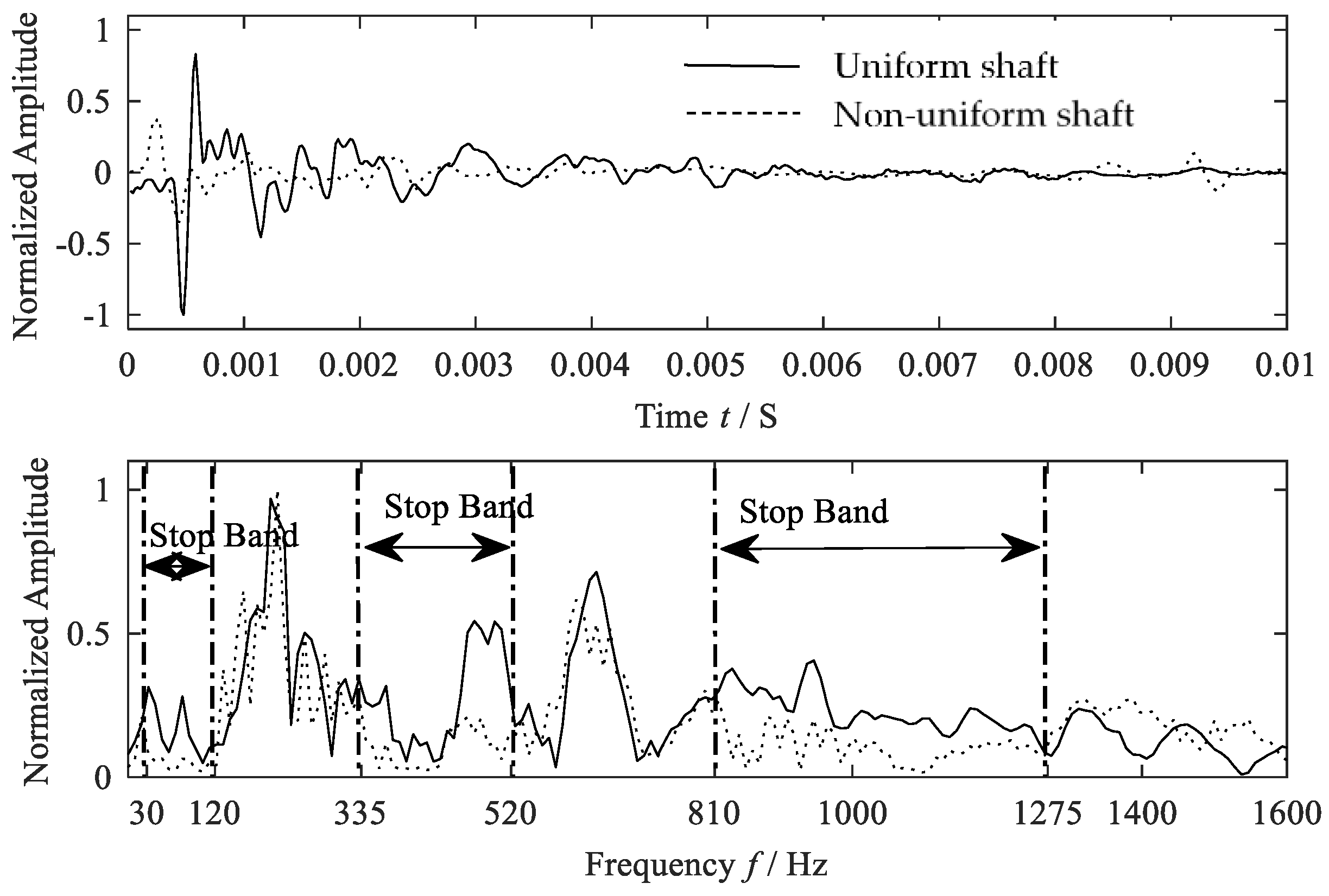
Applsci 08 02105 g006aApplsci 08 02105 g006b
Figure 7. Experimental Stop Bands derived by spectrum comparison.
Applsci 08 02105 g007
Figure 8. Numerical propagation constants derived from different crack locations.
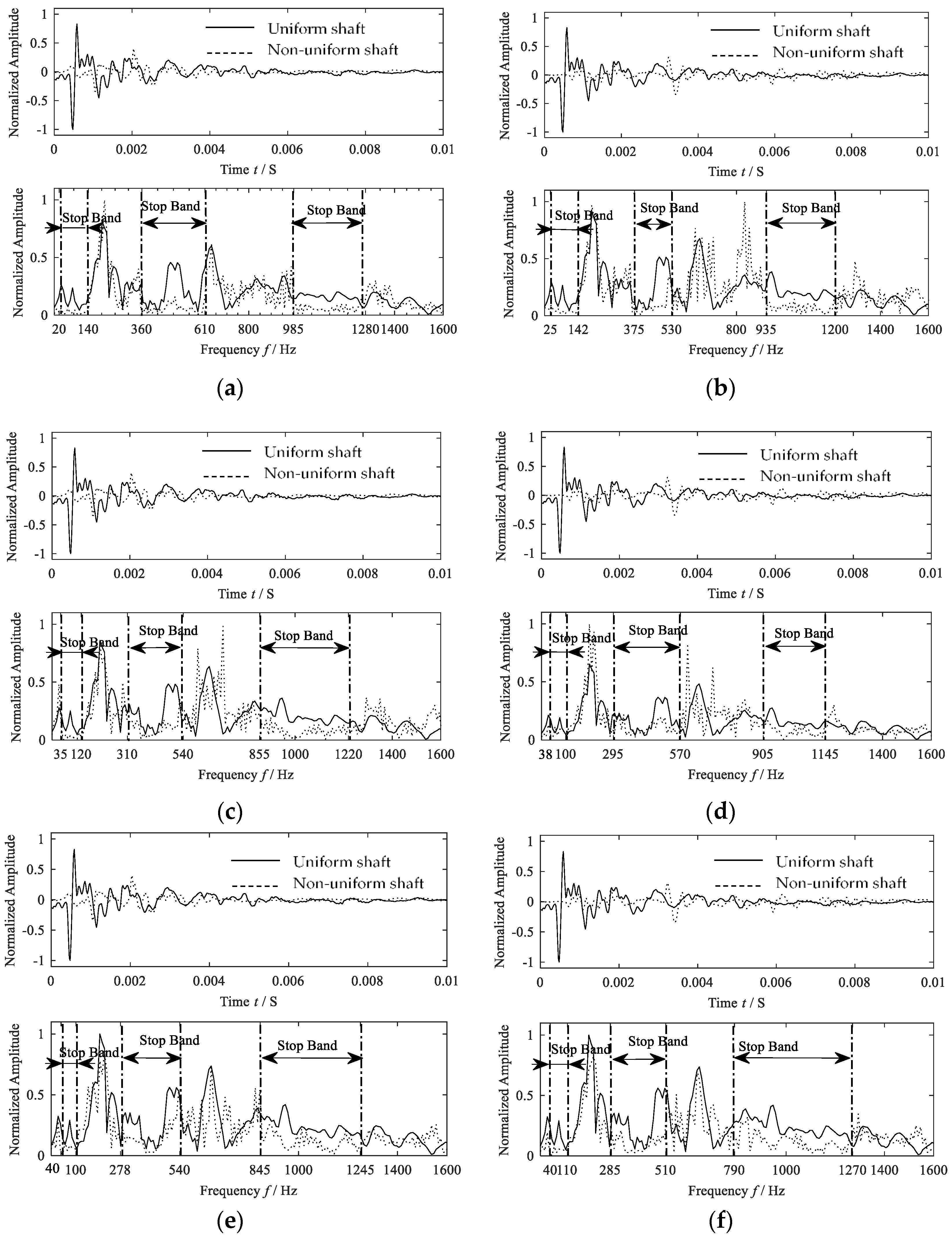
Applsci 08 02105 g008
Figure 9. Experimental Stop Bands derived at different crack locations, where (a) is for location 0.1L, (b) is for location 0.2L, (c) is for location 0.4L, (d) is for location 0.5L, (e) is for location 0.6L, (f) is location 0.7L, (g) is for location 0.8L and (h) is for location 0.9L.
Applsci 08 02105 g009aApplsci 08 02105 g009b
Figure 10. Numerical propagation constants derived from different crack depths.
Applsci 08 02105 g010
Figure 11. Experimental stopbands derived from different crack depth, where (a) is for the case a/Rc = 0.1, (b) is for the case a/Rc = 0.2, (c) is for the case a/Rc = 0.3 and (d) is for the case a/Rc = 0.4.
Applsci 08 02105 g011
Figure 12. Numerical propagation constants derived from different rotating speeds.
Applsci 08 02105 g012
Figure 13. Experimental propagation characteristics derived from different rotating speeds, where (a) is for 0 Hz, (b) is for 10 Hz, (c) is for 20 Hz, (d) is for 30 Hz and (e) is for 40 Hz.
Applsci 08 02105 g013
Table 1. The numerical and experiment scheme.
Location of the Crack (xc) Depth of the Crack (a)RPM (Hz)
Part 10.3L0.5Rc50
Part 20.3L0.1Rc, 0.2Rc, 0.3Rc, 0.4Rc, 0.5Rc50
Part 30.1L, 0.2L, 0.3L, 0.4L, 0.5L, 0.6L, 0.7L, 0.8L, 0.9L0.5Rc50
Part 40.3L0.5Rc0, 10, 20, 30, 40, 50
Table 2. Numerical stopbands derived from different crack modes.
Crack ModeStopbands (Hz)
Mode I[106, 138], [492, 546], [1100, 1261]
Mode II[110, 141], [499, 564], [1157, 1261]
Mode III[34, 124], [346, 516], [826, 1261]
Table 3. Numerical stopbands derived at different crack locations.
Locations Stopbands (Hz)
0.1L[26, 148], [352, 592], [976, 1284]
0.2L[30, 142], [384, 526], [926, 1194]
0.3L[34, 124], [346, 516], [826, 1261]
0.4L[36, 116], [316, 542], [848, 1220]
0.5L[38, 106], [288, 562], [896, 1140]
0.6L[40, 106], [278, 540], [842, 1226]
0.7L[40, 112], [282, 502], [790, 1262]
0.8L[42, 122], [290, 496], [798, 1188]
0.9L[44, 136], [294, 544], [830, 1210]
Table 4. Experimental stopbands derived from different crack locations.
Locations Stopbands (Hz)
0.1L[20, 140], [360, 610], [985, 1280]
0.2L[25, 142], [375, 530], [935, 1200]
0.3L[30, 120], [335, 520], [810, 1275]
0.4L[35, 120], [310, 540], [855, 1220]
0.5L[38, 100], [295, 570], [905, 1145]
0.6L[40, 100], [278, 540], [845, 1245]
0.7L[40, 110], [285, 510], [790, 1270]
0.8L[45, 120], [290, 500], [805, 1195]
0.9L[50, 130], [295, 550], [830, 1220]
Table 5. Numerical Stopbands derived at different crack depths.
Depth (a/Rc)Stopbands (Hz)
0.1[102, 134], [480, 534], [1060, 1261]
0.2[80, 126], [412, 518], [918, 1261]
0.3[58, 124], [372, 516], [860, 1261]
0.4[42, 124], [354, 516], [838, 1261]
0.5[34, 124], [346, 516], [828, 1261]
Table 6. Experimental stopbands derived at different crack depths.
Depth (a/Rc)Stopbands (Hz)
0.1[455, 540], [1000, 1270]
0.2[421, 522], [920, 1270]
0.3[42, 143], [337, 528], [880, 1270]
0.4[35, 130], [335, 525], [850, 1275]
0.5[30, 120], [335, 520], [810, 1275]
Table 7. Numerical stopbands derived from different rotating speeds.
RPMStopbands (Hz)
0 Hz[0, 71], [285, 455], [743, 1181]
10 Hz[0, 82], [297, 467], [758, 1196]
20 Hz[0, 91], [309, 479], [772, 1210]
30 Hz[8, 100], [322, 492], [787, 1225]
40 Hz[23, 113], [332, 502], [808, 1243]
50 Hz [33, 124], [346, 516], [826, 1261]
Table 8. Experimental stopbands derived from different rotating speeds.
RPMStopbands (Hz)
0 Hz[0, 50], [270, 440], [735, 1175]
10 Hz[0, 75], [280, 450], [750, 1185]
20 Hz[0, 80], [305, 480], [760, 1210]
30 Hz[0, 95], [325, 500], [790, 1235]
40 Hz[18, 110], [330, 510], [805, 1250]
50 Hz[30, 120], [335, 520], [810, 1275]

