Sub-Pixel Chessboard Corner Localization for Camera Calibration and Pose Estimation

College of Mechanical and Electrical Engineering, Hunan University of Science and Technology, Taoyuan Rd, Xiangtan 411201, China
*
Author to whom correspondence should be addressed.
Appl. Sci. 2018, 8(11), 2118; https://doi.org/10.3390/app8112118
Submission received: 30 September 2018
/
Revised: 24 October 2018
/
Accepted: 26 October 2018
/
Published: 1 November 2018
(This article belongs to the Special Issue Precision Dimensional Measurements)
Abstract
:This work describes a novel approach to localize sub-pixel chessboard corners for camera calibration and pose estimation. An ideally continuous chessboard corner model is established, as a function of corner coordinates, rotation and shear angles, gain and offset of grayscale, and blurring strength. The ideal model is evaluated by a low-cost and high-similarity approximation for sub-pixel localization, and by performing a nonlinear fit to input image. A self-checking technique is also proposed by investigating qualities of the model fits, for ensuring the reliability of addressing perspective-n-point problem. The proposed method is verified by experiments, and results show that it can share a high performance. It is also implemented and examined in a common vision system, which demonstrates that it is suitable for on-site use.
1. Introduction
Computer vision is an interdisciplinary field that deals with how computers can be made for gaining high-level understanding from digital images or videos. From the perspective of engineering, it seeks to automate assignments that the human eyes can do. As a sub-domain of computer vision, visual measurement is employed for some applications involving dimensional survey tasks, and it always utilizes one or more cameras with exactly known intrinsic parameters for addressing perspective-n-point problem [1] and, therefore, camera calibration is pivotal for ensuring the system accuracy [2].
Most camera calibration approaches require a certain number of correspondences between world and image frames, which are also known as control points, and they usually are called “targets” in photogrammetry [3]. These approaches are performed with planar or non-planar targets with exactly known geometries. After the targets are photographed, their corresponding image points need to be localized for solving intrinsic and extrinsic parameters based on bundle adjustment or other optimization models [4]. As a result, the accuracy of camera calibration is largely dependent on the localization of image points, and usually evaluated by re-projection errors [5].
Circular dots and chessboards are the most common target types. Without a loss of generality, projecting the center of a circle yields an image point that is not necessary to be the center of a pattern projected from the circle, unless the pattern is still circular. Contrarily, the corner of a chessboard is scarcely subjected to projective transformations. For that reason, chessboards are more convenient for achieving targets in visual measurements [6]. In addition, since Zhang [2] proposed a flexible calibration approach employing a planar rig with chessboard patterns, this approach has been cited more than ten thousand times, and made chessboards the most frequently used targets for camera calibration.
Chessboard corners can be detected at pixel level using conventional detectors, such as Harris [7] and Kanade-Lucas-Tomasi (KLT) [8]. These detectors usually extract a set of redundant points from one corner, due to user-defined parameters. Some modified means [9,10,11] are contributed to make arbitrary points converge into nearby corners, but their operational accuracy is still at pixel level. In many application scenarios [12,13,14], however, pixel resolution is not yet accurate enough and, therefore, mathematical techniques, such as interpolations or approximations, are used to localize sub-pixel corners. In this paper, a novel approach for sub-pixel corner localization is proposed, and experiments are conducted to verify the new approach.
2. Related Work
During the last two decades, a quantity of sub-pixel localization approaches have been proposed for ensuring the accuracy of camera calibration and pose estimation, which can be roughly divided into three categories discussed in this section.
2.1. Approaches Based on Image Gradient
Sroba [15] shares a sub-pixel localization technique based on the observation that a vector from a corner to any part of its adjacent area is perpendicular to the image gradient of the corner. Points from the adjacent area are used to apply some mathematical treatments for solving a location iteratively; this location is taken as the new center of the adjacent area, until the center stays within a set threshold. Bok [16] adopts a sub-pixel finder algorithm based on Harris detector. From the given initial corner locations, the algorithm iteratively updates the individual corner locations to the largest gradient values using patch-based structure tensor calculation. The algorithm calculates the structure tensor by directly interpolating the gradients, instead of first interpolating the image and second computing the gradients for reducing computational costs. The first mentioned category has been implemented by a toolbox [17] and a library function [18] and, therefore, frequently employed in many application scenarios. These approaches can achieve high efficiency, but they are sensitive to image noise, and often lead to unstable results for on-site use.
2.2. Approaches Based on Grayscale Symmetry
Chu [19] introduces a sub-pixel detector using a round template under image physical coordinates. The round template is employed to pass through a dilated image, and corners are ultimately determined by calculating the centroid of redundant points based on the symmetry of chessboard patterns. Zhao [20] proposes a method based on the property that the symmetry of a square region is more significant when the central pixel of it is closer to a corner. Symmetric factors of all pixels in a selected area are calculated for obtaining a weighted sub-pixel corner position. These approaches can achieve better results when detecting blurred or overexposed images. However, they need a bigger region of interest (ROI), and come at a higher computation cost due to the determination of symmetric factors using a sliding template or window and, therefore, they are subject to certain constraints of lens distortions and expensive for real-time use.
2.3. Approaches Based on Polynomial Fitting
Lucchese [21] performs a least-squares fit of a quadratic polynomial to a low-pass version of the input image. The approach obtains saddle points from the polynomial coefficients and is invariant to affine transformations. Chen [22] computes intermediate values in the Harris-corner-like detection phase to obtain a second-order Taylor expansion of input image, saddle points are found based on a corner model restricted to orthogonal corners. Mallon [23] proposes an edge-based nonlinear corner localizer. The localizer performs a least-squares fit of a parametric edge model to an edge version of input image. Placht [24] develops a modified strategy inspired by the method mentioned in [21]. A corner is refined to sub-pixel accuracy by filtering the adjacent region around it using a 2-D cone filter for an intensity surface amenable to fitting a quadratic polynomial. On the premise of selecting a reasonably small neighborhood, these approaches can yield a suitable approximation in the presence of nonlinear distortions and projective transformations, due to the affine invariance [25]. However, they require a filtered version of the input image for polynomial fitting, because their corner models are not accurate enough for direct processing, which still need to be optimized for improving reliability and efficiency of sub-pixel localization.
3. Methodology
In this section, an accurate model of chessboard images is established for localizing sub-pixel corners; the methodology is based on polynomial fitting and without being dependent on image filtering.
3.1. Ideally Continuous Corner Model
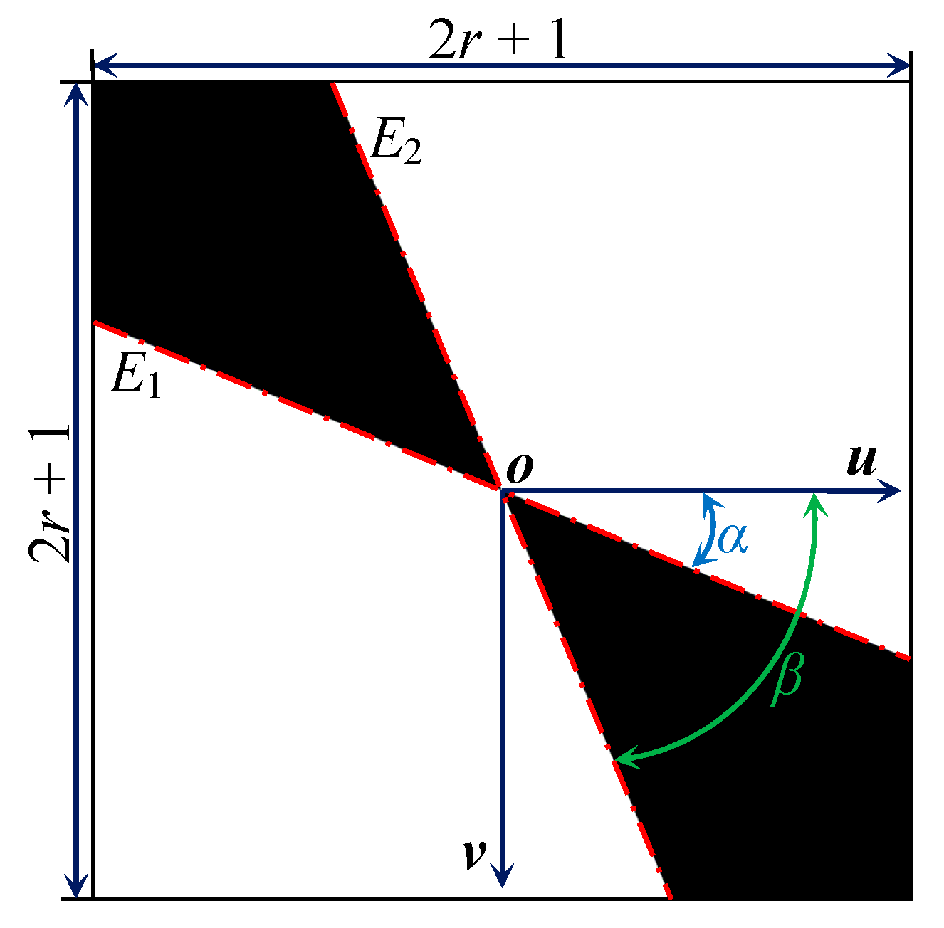
It is intuitive to imagine that a corner is located at a junction of two edges, and has the smallest radius of curvature; pixels around it appear as a high change of brightness in all directions. As represented in Figure 1, a square region C with a center o = [0, 0] and an area of (2r + 1)2 pixels is observed to analyze a chessboard image for the following description. Geometrically, a straight line L passing through o can be given as
where ω is the angle of inclination. Using the sign function sgn(x) yields an ideal edge E related to L via
An ideally continuous chessboard image, with a gray value +1 in the white and −1 in the black regions, is then defined:
where α and β are the angles similar to ω, and determine two edges E1 and E2. It is worth mentioning that Equation (3) is subject to a reasonably small r. Otherwise, E1 and E2 may be re-defined by two curve functions for a suitable approximation of lens distortions.
In actual imaging, however, Ci is inevitably blurred by the lens of a vision system. A point input, represented as a single pixel in Ci, will be reproduced as a spread region in a blurred image Cf. For practical purposes, the blurring response described by the point spread function (PSF) is always approximated by a radio-symmetrical Gaussian kernel [26]. Similarly, Cf is modeled by convolving Ci with a 2-D Gaussian filter:
with σ effectively denoting the blurring strength.
Distinctly, the gray level of Cf is not in the same range as that of a digital image in the common use. Under the assumption that the vision system has a linear response to the light intensity within a reasonable range, Cf can be transformed by
with κ and λ related to the maximum and minimum gray values gmax and gmin of Cs via
3.2. Sub-Pixel Corner Localization
According to the existing techniques discussed in Section 2.3, since a real region R is detected with a known corner position cp = [up, vp] at pixel level, the ideal model, Cs, most similar to R (the highest PSNR), can be found by determining
where μ and υ form a vector d from the ideal corner position to the center of Cs. It is evident that the closed expression of Cf is required to address the above optimization by common means, e.g., the Gauss–Newton method. Despite the fact that Equation (4) cannot be directly analyzed by anti-derivatives, it is approximately evaluated by separating the Gaussian kernel and using integration by parts, given as
where Δ(u, v) is the integral remainder term, erf(x) denotes the Gaussian error function, and θ1 and θ2 are also known as the angles of shear and rotation in image plane. The corner model, approximated in Equations (8) and (9), share a high similarity with the ideal one in Equation (4), due to an effective estimation and compensation of Δ(u, v) (Figure 2).
However, there is still a lack of the closed form for the Gaussian error function; an accurate but expensive way is replacing it by piecewise polynomials [27]. Considering that most applications utilize 8-bit gray images (256 gray-levels), this replacement should be a balance between the computational accuracy and efficiency. Alternatively, a low-cost approximation tanh(ρx) is used, and leads to an acceptable result by selecting a suitable value for the coefficient ρ (Figure 3).
Finally, Equation (7) can be achieved using a linear optimization in iterations. μ and υ are initialized to 0 and σ to 1. α and β are initialized based on edge extraction [28]. κ and λ are initialized using the gray values in the black and white areas close to cp. Generally, about 14 pixels are suitable for r with an overall consideration of the lens distortions, image noise, and computational efficiency. After sufficient iterations for the system convergence, sub-pixel corner cs can be calculated from
3.3. Self-Checking for Perspective-n-Point
Resulting from a maximum likelihood estimation of Cs, the residual εi, j can be used to evaluate the quality of model fit. Let Ё be similar to the root-mean-square error (RMSE), and expressed as
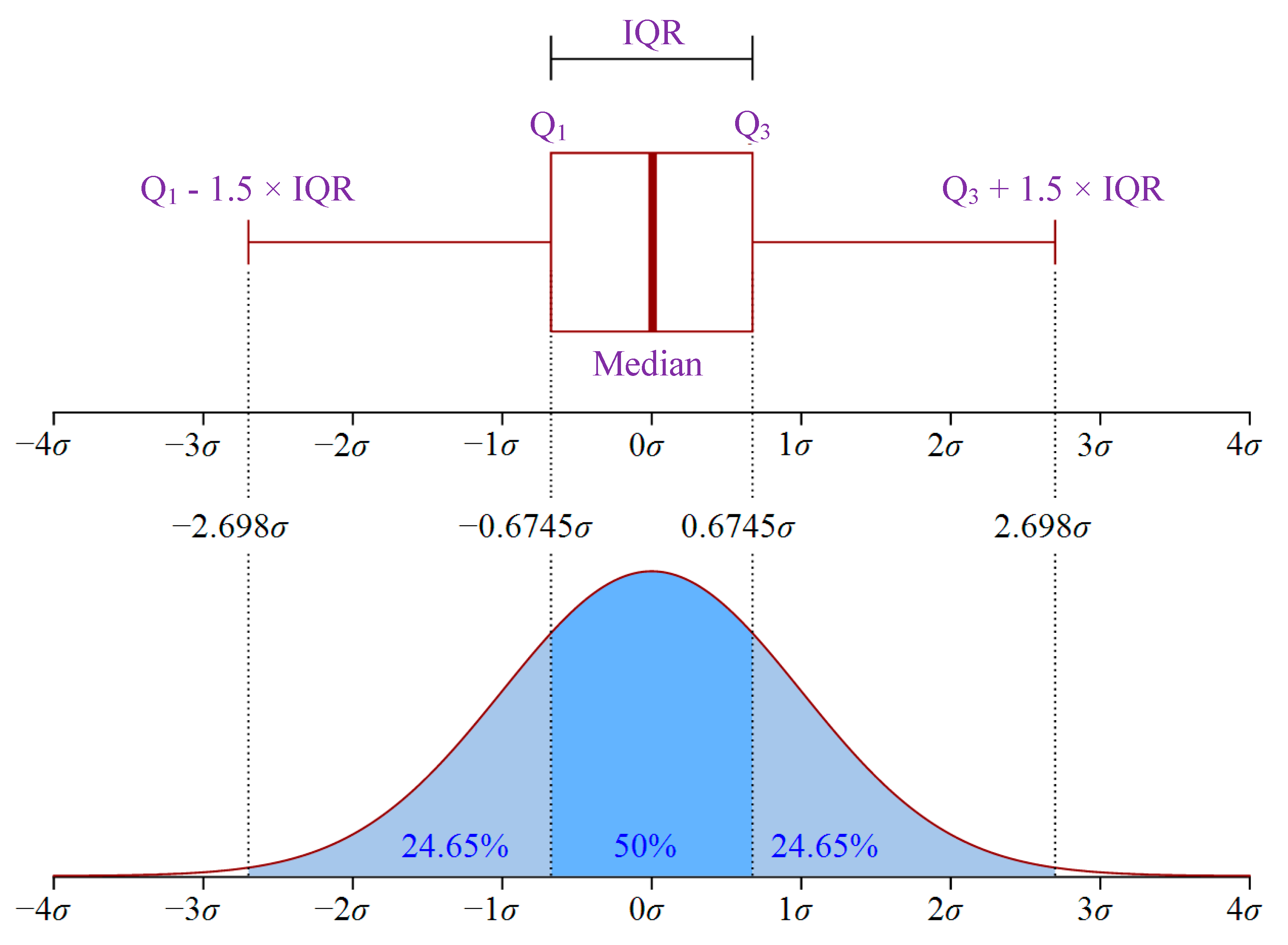
The factor Ё is slightly and unavoidably affected by the lens distortions and image noise, but remarkable when there is a great deal of light pollution (or imbalanced illumination) brought into a chessboard image, which often happens in on-site applications. Thus, it can also be considered as a metric to reflect the reliability of sub-pixel localization. In order to achieve a self-checking technique for perspective-n-point, boxplot analysis is more appropriate than conventional means, e.g., 3-sigma rule [29]. The boxplot distinguishes outliers using quantiles (Figure 4), rather than depending on a prior knowledge about the distribution of actual dataset and, therefore, it has a higher flexibility.
It is assumed that a chessboard image is detected with an array of sub-pixel corners (the array size is M × N). Using Equation (11) gives a corresponding metric Ёm,n for the corner cm,n = [um,n vm,n], m ∈ {1, …, M}, n ∈ {1, …, N}. As illustrated in Figure 4, since the quantiles Q1 and Q3 are obtained by investigating all the metrics, the factor wm,n, standing for the reliability of cm,n, is then determined:
Perspective-n-point is the problem of estimating a 3-D rotation r and a translation t of a calibrated camera, with respect to the world frame. Since the chessboard mentioned above is defined in the world frame accurately, 3-D points in it and their corresponding image points follow a pin-hole model for the camera [2]:
where qm,n is the (m, n)th 3-D point and sm,n the corresponding scale factor. fx and fy are the scaled focal lengths, [u0 v0] is the principal point. An optimal solution of sm,n is related to the given r and t via
Considering wm,n as the penalty factor in association with the above estimator yields
Rodrigues parameters, instead of Euler rotations, are recommended for simplifying the above optimization [30]. It is worth being pointed out that sub-pixel corners obtained according to Section 3.2 cannot be directly taken as image points, which need to be corrected beforehand, due to lens distortions [2].
4. Evaluation
In this section, experiments on synthetic and real datasets are conducted to verify the proposed method with three references detailed in literatures [16,20,24]. In order to decrease the influence on localization result due to different parameter settings, for both the proposed and referenced methods, each chessboard corner is detected with the same initial pixel coordinates, and refined from the same local neighborhood with a square size of 31 × 31 pixels.
4.1. Synthetic Data
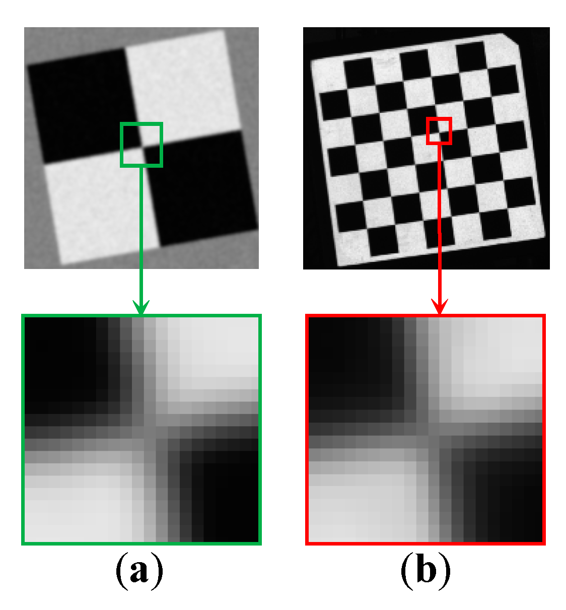
In order to acquire synthetic chessboard image, a pin-hole camera is simulated with the properties: [fx, fy] = [7000, 7000], [u0, v0] = [1296, 972]. The image resolution is set to 2592 × 1944. A single chessboard pattern with 20 mm cell size in both directions is projected to the image plane. Since optical paths are reversible, an ideal projection from the pattern center can be found and defined as ground truth. Gaussian blur with the window parameter σf and Gaussian noise with 0 mean and standard deviation σn are added to make the image similar in appearance to a real one (Figure 5). For each given σf and σn, 100 independent trials are performed, with other simulation parameters varied and limited in their ranges (Table 1), under the premise of ensuring faultless projections.
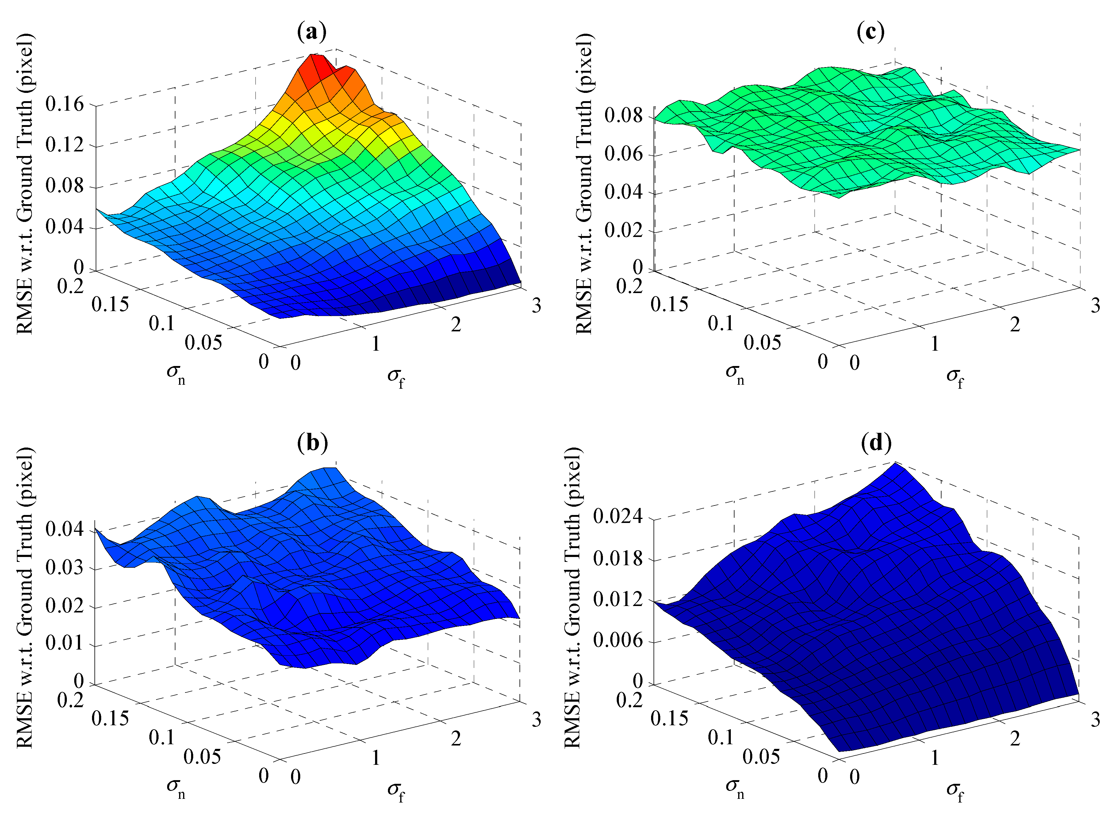
Figure 6 depicts the RMS error of sub-pixel localization as a function of σf and σn. The proposed technique performs significantly better than the referenced ones. Although it results in a higher error due to the increase of σf and σn, the performance drop is not as pronounced as for the others. Concretely, for the poorest image quality (σf = 3, σn = 0.2), the result shows that the errors are about 0.154, 0.041, 0.077, and 0.024 pixels for [16,20,24], and the proposed technique, respectively. Remarkably, Placht et al. [24] yields a stable, but significant, error in the presence of the change of σf and σn for taking filtered images as inputs. That is to say, it not only eliminates noise distinctly, but also leads to an extra uncertainty of sub-pixel localization.
In addition, sub-pixel localization errors from all trials (the total number is 40,000) are gathered for an overall evaluation represented by boxplots. As shown in Figure 7, for the proposed and referenced methods, interquartile ranges (IQRs) are highly symmetrical about medians pretty close to zero. In detail, the IQRs are about 0.18, 0.13, 0.32, and 0.04 pixels in both directions for [16,20,24], and the proposed method, respectively. The smaller IQR reflects the better performance of sub-pixel localization. Again, using filtered images as inputs lead to a particular outcome, that there are no outliers to be distinguished with the largest IQR for [24].
The above simulation relies on the assumption that edges defining a corner are completely straight in the observation area, or region of interest, where the corner is going to be found. However, it is well known that lenses inevitably have distortions. To obtain maximum allowable distortions for the method, another simulation is conducted, with the fixed blur strength and noise level (σf = 1.5, σn = 0.1), and the first order radial distortion with the degree k1 is added to the image (Figure 8). Again, for each given k1, 100 independent trials are performed, with other simulation parameters varied and limited in their ranges (Table 1), except for [tx, ty, tz] set to [115, 80, 1000], for ensuring the projections farther away from the principal point.
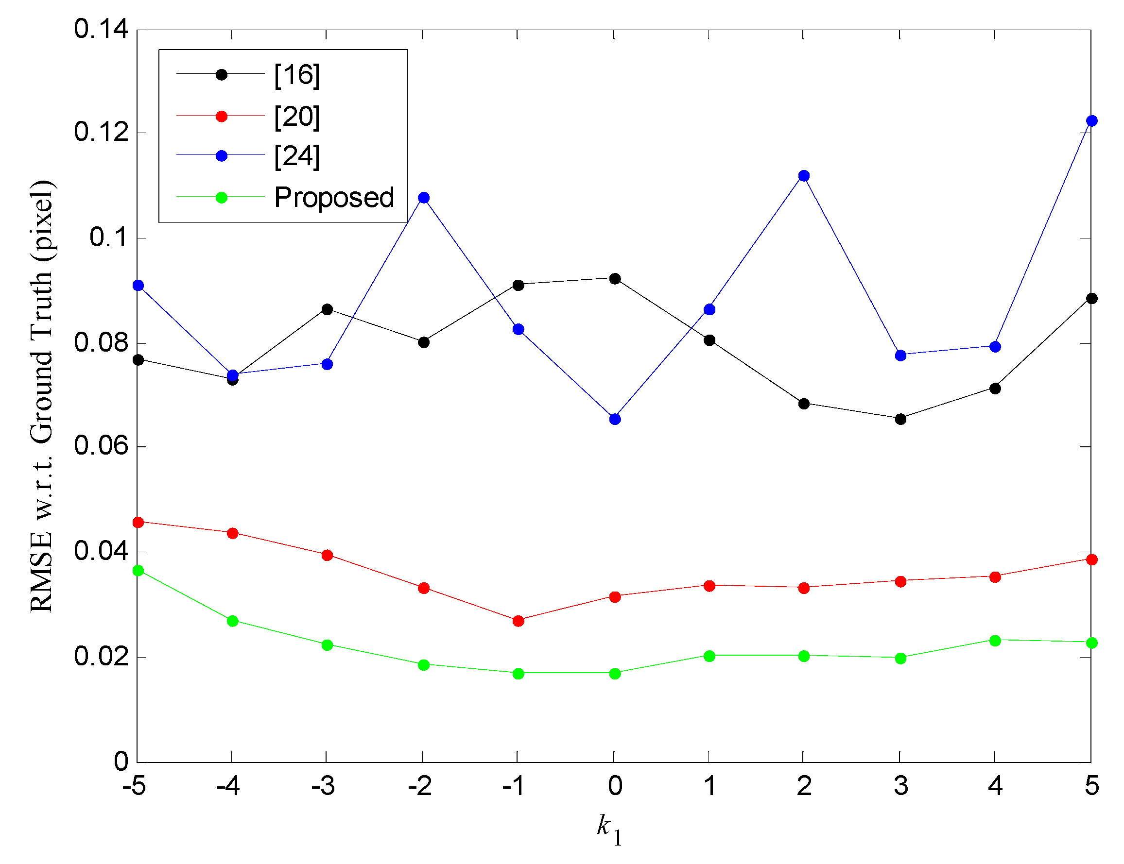
Figure 9 depicts the RMS error of sub-pixel localization as a function of k1. The highest errors are 0.089 pixels for [16], 0.046 pixels for [20], 0.123 pixels for [24], and 0.037 pixels for the proposed method. Again, the proposed method performs significantly better than the referenced ones when k1 varies from −5 to 5. Different from [20] and the proposed method, Bok et al. and Placht et al. [16,24] show a distinct variability due to the limitation of their methodologies; the blur strength and noise level in the simulation have greater impact on the localization result than the distortion. For practical applications, however, cameras with the coefficient k1 larger than 5 are lesser used in photogrammetry because the pinhole model is no longer applicable for them. Therefore, for calibrating a camera for common use, the proposed method can be effectively performed without any pretreatment.
4.2. Real Data
In contrast to simulations, real data experiments cannot directly evaluate the accuracy of sub-pixel localization via the observed corner coordinates, due to their undetermined ground truth data. An alternative and indirect way is examining it based on camera calibration technique. Figure 10 shows that a camera (JPLY, G1GD05C) with 16 mm lens and 2592 × 1944 image resolution is employed for conducting a camera calibration experiment based on a coordinate measuring machine (CMM) (Brown & Sharpe, Global Image 7107) with a single chessboard pattern (20 × 20 mm cell size) mounted on the end of its probe. 3-D control points are achieved by programmatically driving the probe to a set of specially designed positions, and provided with a dimensional error of less than 0.003 mm in both directions. For each position, the chessboard pattern is recorded by the camera for capturing a corresponding corner. Since all corners are located at the sub-pixel level, the camera can be calibrated based on bundle adjustment [4,6].
Table 2 lists the result of intrinsic parameters calibrated from the corners based on four different approaches. According to the definition of radial distortion coefficients detailed in [2], for [16,20,24] and the proposed method, the maximum distortions evaluated using the image point furthest from the principal point are 22.78, 25.92, 29.33, and 24.54 pixels in the radial direction, respectively. Among them, the contributions of k2 are 2.03 pixels for [16], 6.06 pixels for [20], 10.06 pixels for [24], and 4.62 pixels for the proposed method. Therefore, k2 has a much smaller influence on the pixel offsets than k1. Or rather, the estimator of k2 is more sensitive to noise in the corner coordinates. In spite of the fact that the result cannot intuitively demonstrate the performance of each approach, it is pivotal for the following investigations.
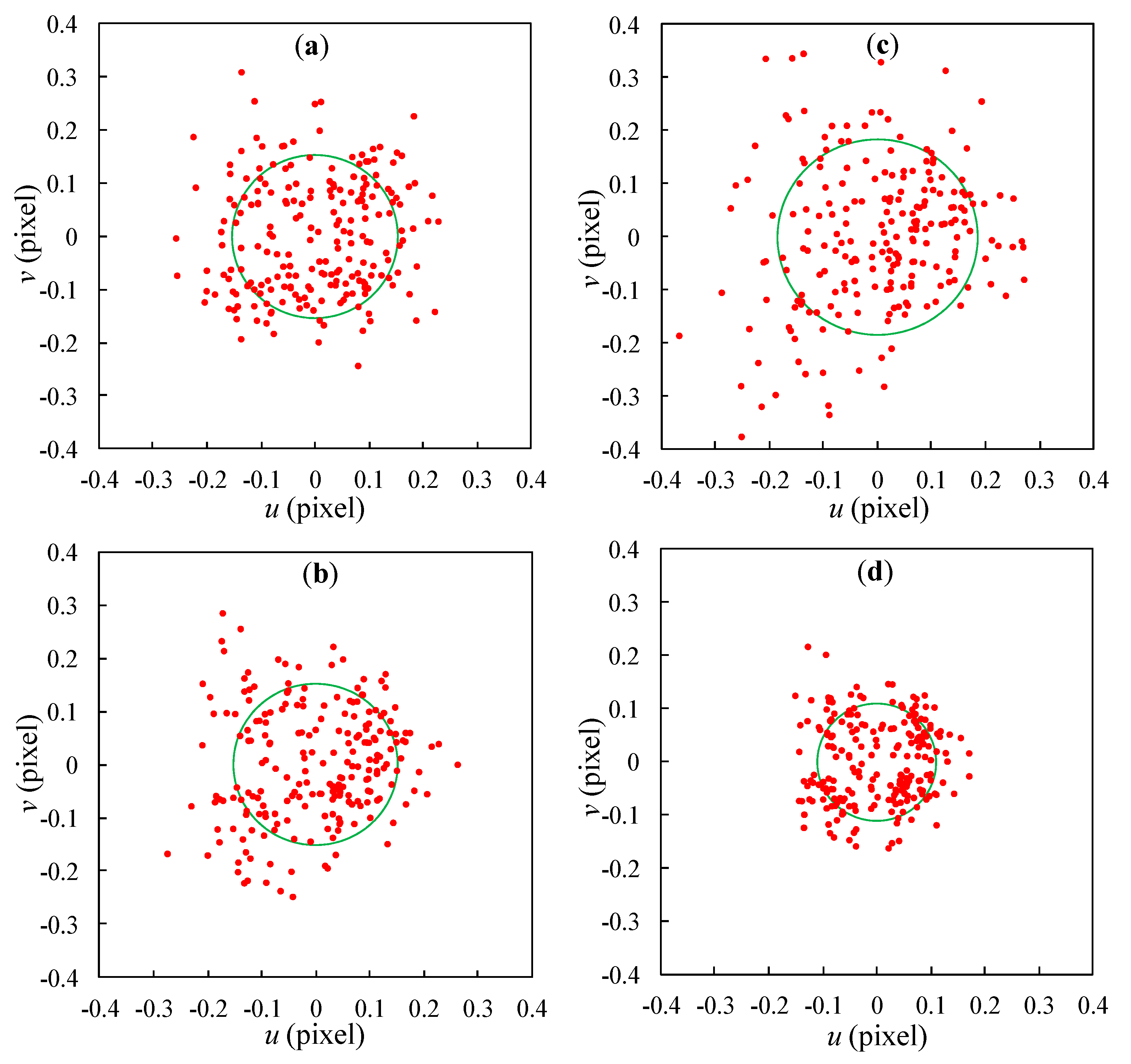
Figure 11 represents four scatter plots of re-projection errors. For general examinations, the maximum and mean re-projection errors for the proposed method are 0.22 pixels and 0.11 pixels, evidently less than 0.32 pixels and 0.15 pixels for [16], 0.29 pixels and 0.15 pixels for [20], 0.39 pixels and 0.18 pixels for [24]. From the standpoint of addressing perspective-n-point problem, the re-projection errors, assessing the validity of calibration, are subjected to some optical indications, e.g., image and lens resolutions, and integrated with certain methodologies, including calibration model, target geometry, and sub-pixel localization. The mentioned experiment employs a robust model with stereo points establishing correspondences between world and image frames accurately and, therefore, the lower re-projection errors not only reflect the better solution of perspective-n-point, but also testify the higher accuracy of sub-pixel localization. Therefore, the corners obtained using the proposed technique are better suited for camera calibration.
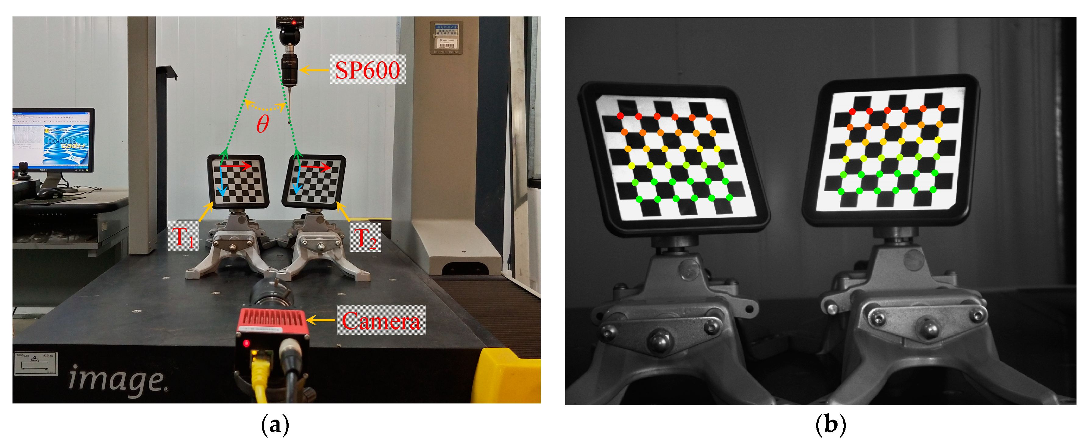
In order to alternatively examine the proposed technique, different measurements on displacement and attitude are carried out using the CMM and camera mentioned above. Firstly, for displacement measurement, a target (6 × 6 grid of points, 20 × 20 mm cell size) fixed on the end of the probe is moved with the guide and imaged by the camera placed in front of the CMM, for measuring a distance d between two different positions as an evaluation factor (Figure 12). Secondly, for attitude measurement, two targets, T1 and T2, mounted on the base with the same grid and cell as that of the above measurement, are imaged by the camera (Figure 13). Among the three axis vectors, only the one in the z direction can be perfectly measured using the probe (Renishaw, SP600), by scanning the pattern plane of each target, due to a restriction that makes it hard to capture 3-D coordinates of a corner accurately, by means of contact measurements. Thus, the included angle θ between two normal vectors is adopted as another evaluation factor more suitably. Fifteen independent trials are performed to localize sub-pixel corners, employing both the proposed and referenced methods, and estimate the camera poses from their respective intrinsic parameters listed in Table 2. The metrics d and θ are then computed for investigating discrepant deviations with respect to the CMM data.
Figure 14 presents the results from the above measurements. Under the premise that the CMM provides baselines with a higher accuracy, the RMS errors of d and θ are 0.032 mm and 0.010° for [16], 0.021 mm and 0.009° for [20], 0.037 mm and 0.013° for [24], and 0.014 mm and 0.006° for the proposed approach. Although there are many estimable and inestimable influences during the experiments, the results are mainly dependent on the accuracies of intrinsic parameters and corner coordinates, and essentially subject to the performance of each sub-pixel localization method because the camera is also calibrated from the respective corner set. From a synthetical point of view, exact values of d and θ are derived from reliable estimations of camera poses predetermined by accurate corner coordinates. As an apparent outcome of the comparison, the proposed technique presents a higher performance than others.
As shown in Figure 15, in order to test the proposed approach in terms of its robustness to real-world data gathering, four images of a stationary chessboard are captured by the mentioned camera under underexposed, overexposed, indoor light interfered, and outdoor light interfered scenarios. For each corner in a 6 × 6 array, its maximin deviation between different scenarios is computed and gathered for an overall evaluation.
Table 3 lists the overall evaluation result for four different approaches. The RMS deviations are 0.419 pixels for [16], 0.287 pixels for [20], 0.396 pixels for [24], and 0.241 pixels for the proposed approach. Considering the fact that the relative pose between the target and camera is stationary, the variability of each detected corner is mainly subject to the robustness of corner localization in the presence of the ambient light changes. The smallest RMS deviation proves that the proposed approach has higher interference immunity, resulting from a more robust corner model.
4.3. Practical Application
The proposed approach is implemented in a visual measurement system called 3D four-wheel aligner (3Excel, T50). The system, designed for aligning four automobile wheels, mainly consists of an upper computer and four cameras and chessboard targets (Figure 16). Each camera is equipped with infrared filter and illuminant, for ensuring a high immunity to the complicated imaging conditions at customer sites. During an initial operation, the automobile under test is driven up to a certain distance by external force. Meanwhile, the cameras C1 to C4 are triggered in synchronous mode to capture image sequences of the targets T1 to T4 mounted on the front-left, front-right, rear-left, and rear-right wheels, respectively. For each image sequence, sub-pixel corners are detected for estimating a wheel attitude with respect to the corresponding camera; two alignment parameters toe-in/toe-out and camber are then determined by decomposing angles of the wheel attitude unified in a global frame defined by the bodywork. During a real-time alignment, the parameters are dynamically calculated from continuous estimations of the wheel attitude changes with respect to their initial values.
As demonstrated in Figure 17, an automobile (Ford Focus) in healthy condition is used for on-site alignment. The introduced aligner can capture chessboard images with black backgrounds due to the usage of infrared filters and illuminants. After finishing the initial operation, the alignment is carried out and divided into two periods: one performs normally, and the other is interfered by infrared pollution sources. During each period, the alignment parameters are incessantly computed based on both the proposed and built-in techniques, until the number of their recorded values reaches 120.
Figure 18 shows two boxplots of total toe-in/toe-out for the front and rear wheel-sets. This parameter, called toe-in for positive and toe-out for negative values, is defined for investigating the symmetry of each wheel-set about the geometric centerline (or thrust line). For both normal and interfered periods, the proposed method results in a median closer to zero and IQR of minor scope, compared with the built-in algorithm. Considering the fact that two total values should be pretty small because of the healthy condition of the automobile, the boxplots prove that the proposed method shows better central tendency, due to the accurate corner localization. When comparing the medians of the proposed method during two periods, the deviations between them are about 0.003° and 0.002° for the front and rear wheel-sets, significantly less than that of the built-in algorithm (0.009° and 0.003°), which also shows that the proposed method has a higher interference immunity resulting from the self-checking technique.
Figure 19 depicts four curve plots of camber as a function of time stamp for the front-left, front-right, rear-left, and rear-right wheel positions, which are divided into two parts, according to two different periods of the alignment. This parameter is defined for measuring the inclination of a wheel with respect to vertical line of the bodywork. Different from toe-in/toe-out, it is separately investigated using the wheel attitude, and weakly restricted to the absolute symmetry about its baseline for the corresponding wheel-set and, therefore, a total value makes poor sense for the evaluation. However, when observing the median change between two periods of each front wheel, there is a strong comparison that the difference is less than 0.003° for the proposed method, and more than 0.008° for the built-in algorithm.
It should be remarked that both methods yield median changes of the rear positions smaller than that of the front ones. This can be found from both Figure 18 and Figure 19, and especially for the built-in technique. There is a logical explanation, as follows: the distances from the front and rear wheels to the infrared pollution source are about 1.5 m and 3.9 m, respectively. The energy of interference is in a state of decay when the distances become larger and, therefore, has no pivotal influence on corner localization and pose estimation for the rear wheels. That is to say, when there is a lack of robust localization technique, a direct way to improve system accuracy is enhancing image quality. Or rather, perspective-n-point is prone to errors if there are outliers in the set of point correspondences. Thus, the self-checking technique can be used in conjunction with existing solutions to make the final solution for the camera pose more robust to outliers.
4.4. Computational Efficiency Test
One hundred real images are obtained using the camera and 6 × 6 chessboard mentioned in Section 4.2, for testing computational efficiency of the proposed method. An optimized dynamic library of it is implemented in C++ code (available online: https://pan.baidu.com/s/1PgRl3qG8HDi49f8n8Jwe3Q), to make a more objective analysis in terms of processing time compared with two mature functions “findChessboardcorners” and “cornerSubPix” built-in OpenCV. The test is run in VS2010 installed on a desktop computer (CPU: Intel Core i7-6700; RAM: DDR4-2133 16GB; HDD: 1TB). All the images are preloaded in the RAM for an undifferentiated access performance, instead of an unstable reading speed of the HDD.
Table 4 lists the result of the processing time for three different algorithms. Although “cornerSubPix” runs two times as fast as the proposed method due to a low-cost computation based on image gradient, it is not essential for real-time detection, because sub-pixel corners are refined from their pixel coordinates located by expensive pretreatments. There is a common view that “findChessboardcorners” has high performance for rough detection. When comparing with two sub-pixel algorithms, however, it costs 41,715 ms, almost 32 and 14 times longer than that of “cornerSubPix” and the proposed algorithm. Therefore, the present efficiency bottleneck is the pixel detection, not the sub-pixel refinement. What can be expected is that this bottleneck is not unbreakable; some state-of-the-art techniques, such as CUDA and multithread computing, are powerful for addressing this kind of problem.
5. Summary
In this work, a new approach is proposed to localize chessboard corners at sub-pixel level. The proposed approach is based on an ideal chessboard model, established as a function of corner coordinates, rotation and shear angles, gain and offset of grayscale, and blurring strength. In order to localize the sub-pixel corner using a nonlinear fit to input image directly, the ideal chessboard model is approximated by a low-cost and high-similarity expression in the closed form. In order to ensuring the reliability of perspective-n-point, a self-checking technique for pose estimation is proposed by investigating qualities of model fits. The proposed approach has the following superiorities: (1) the methodology is effective without being dependent on image filtering employed as the pretreatment in the references; (2) the approximated corner model is more accurate than that in the references and has a high performance; (3) the self-checking technique, in association with existing solutions, is powerful for on-site use.
Author Contributions
Conceptualization, T.Y. and Q.Z. (Qiancheng Zhao); Methodology, T.Y.; Software, X.W.; Writing—review and editing, Q.Z. (Quan Zhou) and T.Y.
Funding
This work was supported by the National Nature Science Foundation of China [No: 51405154, 51275169]; the Hunan Provincial Natural Science Foundation of China [No: 2015JJ5012]; and the Hunan Provincial Innovation Foundation for Postgraduate of China [No: CX2016B545].
Acknowledgments
The authors are very grateful to Shenzhen 3Excel Tech. Co., Ltd. for providing experimental resources and technical supports.
Conflicts of Interest
The authors declare no conflict of interest.
References
- Penate-Sanchez, A.; Andrade-Cetto, J.; Moreno-Noguer, F. Exhaustive Linearization for Robust Camera Pose and Focal Length Estimation. IEEE Trans. Pattern Anal. Mach. Intell. 2013, 35, 2387–2400. [Google Scholar] [CrossRef] [PubMed] [Green Version]
- Zhang, Z. A flexible new technique for camera calibration. IEEE Trans. Pattern Anal. Mach. Intell. 2000, 22, 1330–1334. [Google Scholar] [CrossRef] [Green Version]
- Sužiedelytė-Visockienė, J. Accuracy analysis of measuring close-range image points using manual and stereo modes. Geodesy Cartogr. 2013, 39, 18–22. [Google Scholar] [CrossRef]
- Bundle Adjustment. Available online: http://en.wikipedia.org/wiki/Bundle_adjustment/ (accessed on 5 April 2018).
- Lepetit, V.; Moreno-Noguer, F.; Fua, P. EPnP: An Accurate O(n) Solution to the PnP Problem. Int. J. Comput. Vis. 2009, 81, 155–166. [Google Scholar] [CrossRef] [Green Version]
- Wang, Y.; Yuan, F.; Jiang, H.; Hu, Y. Novel camera calibration based on cooperative target in attitude measurement. Optik 2016, 127, 10457–10466. [Google Scholar] [CrossRef]
- Harris, C.; Stephens, M. A combined corner and edge detector. In Proceedings of the Alvey Vision Conference, Manchester, UK, 31 August–2 September 1988; pp. 147–151. [Google Scholar]
- KLT: An Implementation of the Kanade-Lucas-Tomasi Feature Tracker. Available online: http://cecas.clemson.edu/~stb/klt/ (accessed on 26 October 2018).
- Escalera, A.D.; Armingo, J.M. Automatic chessboard detection for intrinsic and extrinsic camera parameter calibration. Sensors 2010, 10, 2027–2044. [Google Scholar] [CrossRef] [PubMed] [Green Version]
- Tu, D.; Zhang, Y. Auto-detection of chessboard corners based on grey-level difference. Opt. Precis. Eng. 2011, 19, 1360–1365. [Google Scholar]
- Liu, Y.; Liu, S.; Cao, Y.; Wang, Z. Automatic chessboard corner detection method. IET Image Process 2016, 10, 16–23. [Google Scholar] [CrossRef]
- Yang, S.; Scherer, S.A.; Yi, X.; Zell, A. Multi-camera visual SLAM for autonomous navigation of micro aerial vehicles. Robot. Auton. Syst. 2017, 93, 116–134. [Google Scholar] [CrossRef]
- Song, L.; Wang, M.; Lu, L.; Huan, H. High precision camera calibration in vision measurement. Opt. Laser Technol. 2007, 39, 143–1420. [Google Scholar] [CrossRef]
- Zhang, T.; Liu, J.; Liu, S.; Tang, C.; Jin, P. A 3D reconstruction method for pipeline inspection based on multi-vision. Measurement 2017, 98, 35–48. [Google Scholar] [CrossRef]
- Sroba, L.; Ravas, R.; Grman, J. The Influence of Sub-pixel Corner Detection to Determine the Camera Displacement. Procedia Eng. 2015, 100, 834–840. [Google Scholar] [CrossRef]
- Bok, Y.; Ha, H.; Kweon, I.S. Automated checkerboard detection and indexing using circular boundaries. Pattern Recognit. Lett. 2016, 71, 66–72. [Google Scholar] [CrossRef]
- Camera Calibration Toolbox for Matlab. Available online: http://www.vision.caltech.edu/bouguetj/calib_doc/ (accessed on 1 September 2018).
- Camera Calibration and 3D Reconstruction. Available online: http://docs.opencv.org/2.4/modules/imgproc/doc/ (accessed on 5 September 2018).
- Chu, J.; Lu, A.G.; Wang, L. Chessboard corner detection under image physical coordinates. Opt. Laser Technol. 2013, 48, 599–605. [Google Scholar] [CrossRef]
- Zhao, Q.; Chen, Z.; Yang, T.; Zhao, Y. Detection of sub-pixel chessboard corners based on gray symmetry factor. In Proceedings of the SPIE Ninth International Symposium on Precision Engineering Measurement and Instrumentation, Changsha, China, 8–11 August 2014; Volume 9446, p. 94464S. [Google Scholar]
- Lucchese, L.; Mitra, S.K. Using saddle points for sub-pixel feature detection in camera calibration targets. In Proceedings of the Asia-Pacific Conference on Circuits and Systems, Denpasar, Indonesia, 28–31 October 2002; Volume 2, pp. 191–195. [Google Scholar]
- Chen, D.; Zhang, G. A New Sub-Pixel Detector for X-Corners in Camera Calibration Targets. In Proceedings of the 13th International Conference in Central Europe on Computer Graphics, Visualization and Computer Vision, Plzen, Czech Republic, 31 January–4 February 2005. [Google Scholar]
- Mallon, J.; Whelan, P.F. Which pattern? biasing aspects of planar calibration patterns and detection methods. Pattern Recognit. Lett. 2007, 28, 921–930. [Google Scholar] [CrossRef]
- Placht, S.; Fürsattel, P.; Mengue, E.A.; Hofmann, H.; Schaller, C.; Balda, M.; Angelopoulou, E. ROCHADE: Robust Checkerboard Advanced Detection for Camera Calibration. In Proceedings of the European Conference on Computer Vision, Zurich, Switzerland, 6–12 September 2014; Fleet, D., Pajdla, T., Schiele, B., Tuytelaars, T., Eds.; Springer: Cham, Switzerland, 2014. [Google Scholar]
- Alturki, A.S.; Loomis, J.S. X-Corner Detection for Camera Calibration Using Saddle Points. In Proceedings of the International Conference on Image Analysis and Processing, Boston, MA, USA, 25–26 April 2016. [Google Scholar]
- Wang, C.; Sun, T.; Wang, T.; Miao, X.; Wang, R. Multi-PSF fusion in image restoration of range-gated systems. Opt. Laser Technol. 2018, 103, 219–225. [Google Scholar] [CrossRef]
- Chang, S.H.; Cosman, P.C.; Milstein, L.B. Chernoff-Type Bounds for the Gaussian Error Function. IEEE Trans. Commun. 2011, 59, 2939–2944. [Google Scholar] [CrossRef]
- Wang, Z.; Wu, W. Recognition and location of the internal corners of planar checkerboard calibration pattern image. Appl. Math. Comput. 2007, 185, 894–906. [Google Scholar] [CrossRef]
- Hubert, M.; Vandervieren, E. An adjusted boxplot for skewed distribution. Comput. Stat. Data Anal. 2008, 52, 5186–5201. [Google Scholar] [CrossRef]
- Yang, T.; Zhao, Q.; Wang, X.; Huang, D. Accurate calibration approach for non-overlapping multi-camera system. Opt. Laser Technol. 2018. [Google Scholar] [CrossRef]
Figure 1.
Definition of a chessboard image.

Figure 2.
Gray images simulated by the ideal model, approximated model, and Δ(u, v), with different values of θ1 and θ2. The image size is 41 × 41 pixels, σ = 4.
Figure 2.
Gray images simulated by the ideal model, approximated model, and Δ(u, v), with different values of θ1 and θ2. The image size is 41 × 41 pixels, σ = 4.

Figure 3.
Function curve plots of (a): y = erf(x) (dashed), y = tanh(ρx) (solid), and (b): y = tanh(ρx) − erf(x). The coefficient ρ is set to 1.0 (red), 1.1 (purple), and 1.2 (green).
Figure 3.
Function curve plots of (a): y = erf(x) (dashed), y = tanh(ρx) (solid), and (b): y = tanh(ρx) − erf(x). The coefficient ρ is set to 1.0 (red), 1.1 (purple), and 1.2 (green).

Figure 4.
Boxplot with respect to a probability density function of N(0, σ2).

Figure 5.
Chessboard images captured by (a) simulation and (b) real device.

Figure 6.
Localization error with respect to blur strength σf and noise level σn for (a) [16], (b) [20], (c) [24], and (d) the proposed technique.

Figure 7.
Boxplots of the errors between localized and standard values in u (red boxes) and v (blue boxes) directions, regarding (a) [16], (b) [24], (c) [20], and (d) the proposed method.

Figure 8.
Chessboard image captured by simulation with the first order radial distortion, k1 = −5.

Figure 9.
RMS error between localized and standard values as a function of k1 for four different approaches.
Figure 9.
RMS error between localized and standard values as a function of k1 for four different approaches.

Figure 10.
Camera calibration using (a) single chessboard and CMM for achieving (b) 3-D control points with specially designed positions.
Figure 10.
Camera calibration using (a) single chessboard and CMM for achieving (b) 3-D control points with specially designed positions.

Figure 11.
Scatter plots of re-projection errors (red dots) for (a) [16], (b) [20], (c) [24], and (d) proposed method. In each sub-figure, green circle is rendered with a radius equal to the mean re-projection error.

Figure 12.
Experiment for measuring displacement. (a) Determining d via CMM and camera. (b) A merged image of two positions with located corners.
Figure 12.
Experiment for measuring displacement. (a) Determining d via CMM and camera. (b) A merged image of two positions with located corners.

Figure 13.
Experiment for measuring attitude. (a) Determining θ via CMM and camera. (b) One shot in 15 trials with located corners.
Figure 13.
Experiment for measuring attitude. (a) Determining θ via CMM and camera. (b) One shot in 15 trials with located corners.

Figure 14.
Measurement results of (a) displacement d and (b) attitude angle θ.

Figure 15.
Four images of a stationary chessboard captured under (a) underexposed, (b) overexposed, (c) indoor light interfered, and (d) outdoor light interfered scenarios.
Figure 15.
Four images of a stationary chessboard captured under (a) underexposed, (b) overexposed, (c) indoor light interfered, and (d) outdoor light interfered scenarios.

Figure 16.
3D four-wheel alignment. (a) System composition. (b) Initial operation.

Figure 17.
On-site aligning experiment. (a) Using infrared light as pollution source. (b) One shot in image sequence with located corners for each wheel position.
Figure 17.
On-site aligning experiment. (a) Using infrared light as pollution source. (b) One shot in image sequence with located corners for each wheel position.

Figure 18.
Boxplots of (a) front and (b) rear toe-in/toe-out values for the proposed (red boxes) and built-in (blue boxes) techniques. Regarding normal and interfered periods.
Figure 18.
Boxplots of (a) front and (b) rear toe-in/toe-out values for the proposed (red boxes) and built-in (blue boxes) techniques. Regarding normal and interfered periods.

Figure 19.
Camber as a function of time stamp for each wheel position. Solid curves (dashed lines) in red and blue denote function values (medians) for the proposed and built-in techniques, respectively. Regarding normal and interfered periods.
Figure 19.
Camber as a function of time stamp for each wheel position. Solid curves (dashed lines) in red and blue denote function values (medians) for the proposed and built-in techniques, respectively. Regarding normal and interfered periods.


Table 1.
Range set of simulation parameters. yaw, pitch, and roll are the Euler angles related to r. tx, ty, and tz are the dimensional elements of t.
Table 1.
Range set of simulation parameters. yaw, pitch, and roll are the Euler angles related to r. tx, ty, and tz are the dimensional elements of t.
| gmax | gmin | yaw, pitch, roll | tx (mm) | ty (mm) | tz (mm) |
|---|---|---|---|---|---|
| [191, 255] | [0, 63] | [−π/4, π/4] | [−40, 40] | [−30, 30] | [950, 1050] |
Table 2.
Calibration result for four different approaches. k1 and k2 denote the 1st and 2nd order radial distortion coefficients.
Table 2.
Calibration result for four different approaches. k1 and k2 denote the 1st and 2nd order radial distortion coefficients.
| [u0, v0] | [fx, fy] | [k1, k2] | |
|---|---|---|---|
| [16] | [1344.42, 937.37] | [7296.06, 7298.85] | [0.2332083, 0.4313581] |
| [20] | [1342.78, 936.71] | [7298.67, 7302.12] | [0.2237942, 1.2905459] |
| [24] | [1340.02, 937.04] | [7297.59, 7300.76] | [0.2118124, 2.2750773] |
| Proposed | [1343.70, 936.62] | [7299.13, 7302.50] | [0.2253345, 0.9926340] |
Table 3.
Overall evaluation result for four different approaches.
| [16] | [20] | [24] | Proposed | |
|---|---|---|---|---|
| RMSD (pixel) | 0.419 | 0.287 | 0.396 | 0.241 |
Table 4.
Processing time of detecting 100 chessboard images for three different algorithms.
| findChessboardcorners | cornerSubPix | Proposed | |
|---|---|---|---|
| Time (ms) | 41,715 | 1296 | 3051 |
© 2018 by the authors. Licensee MDPI, Basel, Switzerland. This article is an open access article distributed under the terms and conditions of the Creative Commons Attribution (CC BY) license (http://creativecommons.org/licenses/by/4.0/).
Share and Cite
MDPI and ACS Style
Yang, T.; Zhao, Q.; Wang, X.; Zhou, Q. Sub-Pixel Chessboard Corner Localization for Camera Calibration and Pose Estimation. Appl. Sci. 2018, 8, 2118. https://doi.org/10.3390/app8112118
AMA Style
Yang T, Zhao Q, Wang X, Zhou Q. Sub-Pixel Chessboard Corner Localization for Camera Calibration and Pose Estimation. Applied Sciences. 2018; 8(11):2118. https://doi.org/10.3390/app8112118
Chicago/Turabian StyleYang, Tianlong, Qiancheng Zhao, Xian Wang, and Quan Zhou. 2018. "Sub-Pixel Chessboard Corner Localization for Camera Calibration and Pose Estimation" Applied Sciences 8, no. 11: 2118. https://doi.org/10.3390/app8112118
Note that from the first issue of 2016, this journal uses article numbers instead of page numbers. See further details here.