Aircraft Air Compressor Bearing Diagnosis Using Discriminant Analysis and Cooperative Genetic Algorithm and Neural Network Approaches

Abstract

Monitoring and diagnosis of rotating machines has become an effective and indispensable tool for the efficient and timely detection of defects, avoiding then incidents that can have serious economic and human consequences. Bearings are the most sensitive parts of these machines; this is why special attention must be paid to its monitoring. This paper presents a methodology for diagnosing an aircraft air compressor bearing using neural networks that have been optimized by genetic algorithms. We used in our study a database of vibratory signals that were recorded on a test bench from bearings with different defects. The faults features are extracted from these noisy signals using the estimate of the spectral density. The diagnostic capacity of obtained model has been demonstrated by a comparative study with two other automatic classifiers, which are discriminant analysis and neural networks whose training has been done with the Back-Propagation algorithm. This approach has the advantage of simultaneously ensuring the optimal structure of the neural network and accomplishing its learning. The importance of this study is the construction of a diagnostic tool that is characterized by efficiency, speed of decision making and ease of implementation not only on the computers on the ground, but also on the mounted calculators on aircraft.

1. Introduction

Rotating machines play an important role in industrial and transport applications. They have become more complicated, precise and costly. Thanks to technological progress, fault diagnosis techniques, are increasingly being used. Most rotating machines operate by means of bearings, gears and other rotating parts which can often cause defects. These defects can lead the machine to fail, reducing performance and even causing very serious accidents [1,2,3].

Bearings are the most critical elements parts of rotating machines because they support the dynamic forces of a shaft. Therefore they must be closely monitored to detect and locate defects at an early stage.

By using some vibration signal processing methods, it is possible to obtain decisive diagnostic information. These methods are used to characterize, extract and identify fault signatures. Many conventional techniques such as time domain analysis and Fourier analysis are investigated in recent research and performed in many applications. The method, based on scalar features such as Root Mean Square, Crest Factor, and Kurtosis, can detect the presence of faults and their locations but the diagnosis is still imprecise [4,5]. The second approach is based on the application of the Fast Fourier Transform algorithm. However, the total spectrum of the vibration signal (shaft and bearings) obtained does not exhibit an obvious characteristic frequency generated by the defects. This technique is quite limited and it works efficiently only for periodic signals [6].

The autocorrelation function is a statistical average suitable for characterizing random signals in the time domain. The Fourier transform of the autocorrelation function is the Power Spectral Density (PSD). It gives the power distribution of a signal in the frequency domain and is used to characterize random signals. The Welch power density estimation gives the spectral characteristics of signals characterized as random processes [7,8].

However, continuous monitoring of the damage indicative variables is tedious because it is a procedure that requires a good deal of expertise to successfully apply them. It is therefore necessary to have simpler approaches that enable relatively low-skilled operators to make reliable decisions in the absence of diagnostic experts.

Statistical techniques such as Principal Component Analysis (PCA), Linear Discriminant Analysis (LDA) were the first to be used in this field [9,10,11]. The Random Forest Algorithms are based on the decision trees classifier; it has been considered significantly in development of fault machine diagnostics methods through a powerful method for classification and predictions [12,13,14]. Support Vector Machine (SVM) is also used; it is a very precise classifier, robust to noise and overfitting, but expensive in terms of computation [15,16].

Subsequently, artificial intelligent techniques, such as Genetic Algorithms, Fuzzy Logic, and Artificial Neural Networks, have been applied successfully to automatic detection and to diagnosis [17,18,19,20,21,22,23,24,25,26].

In this paper, we aim to diagnose vibration failure occurring on a bearing mounted on the aircraft air compressor. This study concerns two aspects: we seek first to acquire the vibratory signals and to characterize the defects of the compressor bearing. The chosen signal analysis method is the Welch spectral density estimate for its efficiency on signals embedded in noise. The second part allows building a model which facilitates the monitoring and the diagnosis.

We used neural networks with optimization based on genetic algorithms. The diagnostic results obtained by this approach were compared with two other traditional diagnostic methods.

The first model that has been tried is based on statistical methods. The results obtained motivate the choice of another more efficient approach based on Artificial Neural Network.

Then we used neural networks with the Back-Propagation algorithm to accomplish the training. We had to perform several tests with changing at each time the number of neurons in the hidden layer. This method is tedious and it is not sure to find the optimal architecture and the best performance.

To overcome this problem, genetic algorithms have been used. This optimizer uses all the search space to find the neural network architecture that will give the maximum classification rate. This hybrid method of neural networks and genetic algorithms has the advantage of performing both learning and optimization of the network architecture. The results of the diagnosis were very satisfactory.

This method is distinguished from previous work and research by the efficiency, speed of calculations and the option of being implemented in flight systems.

To address the issues discussed above, this paper is organized as follows: Section 2 describes the case of study, the experimental set-up and the vibration signals processing with the method of Welch spectral density estimation. Section 3 is devoted to a brief description of the Linear Discriminant Analysis, Artificial Neural Networks techniques and Genetic Algorithm. The results of the vibration signal processing and the use of these fault monitoring methods are discussed in Section 4. Finally, the main conclusions of this paper are given in Section 5.

2. Data and Signal Processing

The data used in our investigation were recorded on a test bench of an aircraft turbojet engine. Two accelerometers are used to measure vibration in front and rear bearing housing. We used only the signals acquired at the accelerometer mounted on the front bearing housing since the faults to be considered are located at turbojet air compressor bearing.

The acquisition of the signals was carried out through 348 experiments on healthy bearings and defective bearings. These experiments are classified into 4 groups:

• 60 were fault-free
• 96 had inner race bearing fault
• 96 had outer race bearing fault
• 96 had ball bearing fault.

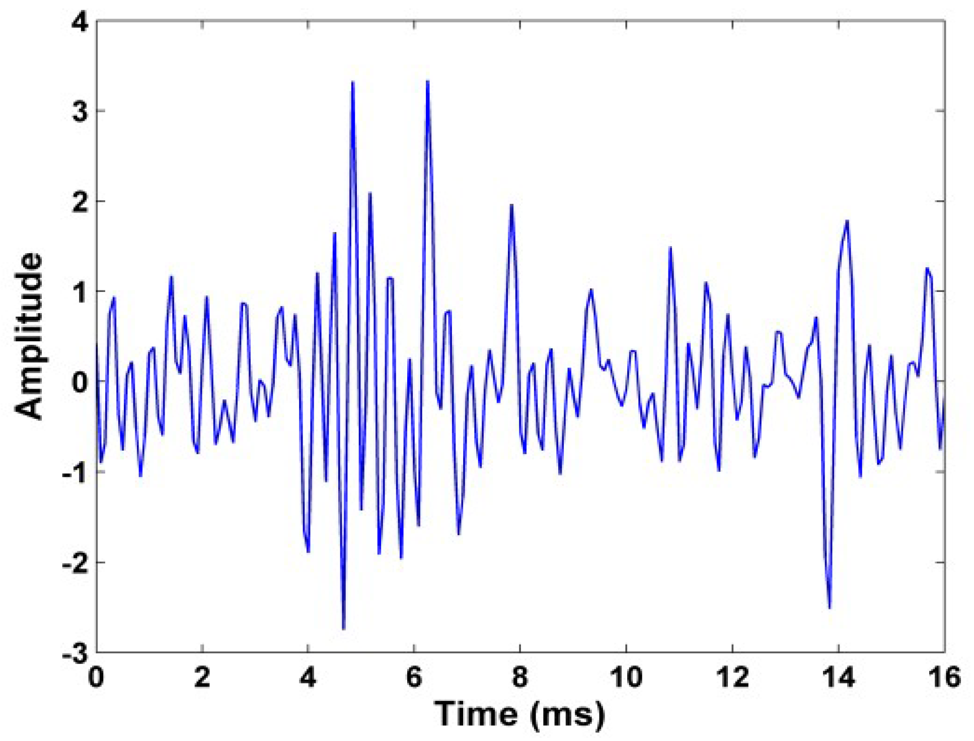
All the signals recorded with a sampling frequency equal to 12,000 Hz. To increase the number of elements in each class, we divided each signal into 3 segments. We got 1044 signal overall. An illustration in the time domain of an inner ring faulty bearing signal is illustrated in Figure 1.

Estimating spectral power density is a very important area in the field of digital signal processing. This study explores the Welch estimation method. It is a nonparametric method which provides a consistent estimator of power spectral density [27]. This method consists to subdividing the records, taking modified periodograms for each subdivision and averaging these modified periodograms. In many cases, this method requires less calculation than other methods because it involves transforming the signal into shorter sequences.

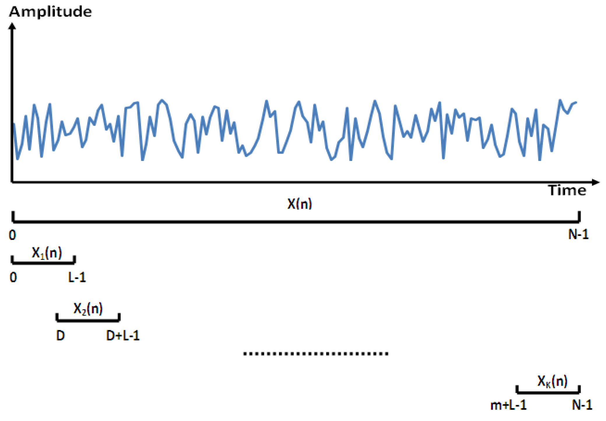
For X(n), a second-order stationary random discrete signal of zero mean $\left(n = 0, 1, 2,\dots , N-1\right)$, we take overlapping segments of length L. The starting points of these segments are multiples of D as illustrated in Figure 2. We assume that we have K segments, $X_1\left(n\right), X_2\left(n\right),\dots , X_K\left(n\right)$ and that they cover the entire record, as described in Equation (1).

$$\begin{gathered} \left(K-1\right) D + L = N \\ X_1\left(n\right)=X\left(n\right) \\ X_2\left(n\right) =X\left(n+D\right) \\ \dots \\ X_K\left(n\right) =X\left(n+\left(K-1\right)D\right) \end{gathered}$$

(1)

To obtain the spectral estimation, we calculate first a dependent frequency (f) modified periodogram ${\widehat{P}}_m^{\left(i\right)}$ for each segment,

$${\widehat{P}}_m^{\left(i\right)}\left(f\right)=\frac{1}{LV}{\left\{{\displaystyle \sum }_{n=0}^{L-1}{W}_S\left(n\right)X\left(n+iD\right)\exp \left(-2\pi jnf\right)\right\}}^2$$

(2)

where $W_s\left(n\right)$ is the window function and V is defined in (3).

$$V=\frac{1}{n}{\displaystyle \sum }_{n=0}^{N-1}{\left|W_s\left(n\right)\right|}^2$$

(3)

The spectral estimate ${\widehat{P}}_{W_S}\left(f\right)$ is the average of these periodograms as given in (4).

$${\widehat{P}}_{W_S}\left(f\right)=\frac{1}{K}{\displaystyle \sum }_{i=0}^{K-1}{\widehat{P}}_m^{\left(i\right)}\left(f\right)$$

(4)

Finally:

$${\widehat{P}}_{W_S}\left(f\right)= \frac{1}{KLV}{\displaystyle \sum }_{i=0}^{K-1}{\left\{{\displaystyle \sum }_{n=0}^{L-1}{W}_S\left(n\right)X\left(n+iD\right)\exp \left(-2\pi jnf\right)\right\}}^2$$

(5)

Thus, the estimation of the spectrum consists in estimating ${\widehat{P}}_{W_S} \left(f\right)$ from a finite number of noisy data. Welch’s method reduces noise at the expense of frequency resolution [28].In our case, we used the hamming window function with a length 100 and an overlap of 30.

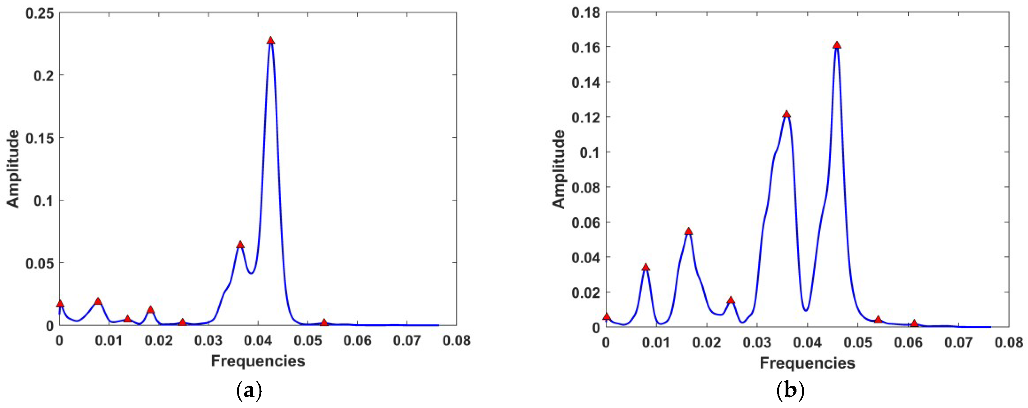
The representation of the spectral density of 2 faulty bearings signals are illustrated in Figure 3. (Frequency and Amplitude are normalized).

After analyzing the 1044 available signals, we extracted the 8 most predominant peaks of the power spectral density (pointed out by triangles in Figure 3). Two values were used for each peak: the characteristic frequency and the value of the spectral density, which gave 16 features for each signal. The data were then organized in a matrix of 16 columns and 1044 rows.

If the generated data is used directly without any processing before starting the training phase, the input variables of the highest value may tend to suppress the influence of the most small. Thus, normalized data will be treated with the same priority. We normalized each line of the data matrix. The 16 features of each line were then scaled between −1 and 1.

After this step, the data was then subdivided into two parts to build the LDA model (60% for learning and 40% for testing) and three parts for building the two others models based on neural networks (60% for learning, 20% for validation and 20% for tests).

3. Methodology

To construct a diagnostic model that automatically classifies defects, three techniques were used: Linear Discriminant Analysis and two other different techniques of Artificial Neural Networks.

3.1. Linear Discriminant Analysis (LDA) Method

LDA is a classification method that has been successfully applied in many fields. For a sample of n observations distributed in M groups, the objective of the LDA is to produce a new representation space where we can better distinguish the M groups [29,30]. It uses the between-class scatter matrix $S_B$ to evaluate the separability of different classes and within-class scatter matrix $S_W$ evaluates the compactness within each class.

Let $X=\left(x_1, x_2,\dots , x_n\right)$ be the training set, each $x_i$ xi belongs to a class $C_l\left(l=1, 2,\dots ,M\right)$.

Between-class scatter matrix $S_B$, within-class scatter matrix $S_W$, and total-class scatter matrix S are defined by (6), (7) and (8).

$$S_W={\displaystyle \sum }_{\mathrm{l}=1}^{\mathrm{M}}{\displaystyle \sum }_{\mathrm{i}=1}^{{\mathrm{n}}_{\mathrm{l}}}(x_i-{\mu }_l)(x_i-{\mu }_l{)}^{\prime }$$

(6)

$$S_B={\displaystyle \sum }_{l=1}^M\left({\mu }_l-\mu \right)({\mu }_l-\mu {)}^{\prime }$$

(7)

$$S=S_w+S_B$$

(8)

with:

• $n_l$ is the number of data points in class L,
• ${\mu }_l$: The center of gravity of class L,
• $\mu$: The center of gravity of all observation.

The principle of LDA is to find vector projection $v_1$ that maximizes the ratio: between-class/within-class scatter. For this purpose, the objective function of LDA is defined by (9).

$$F\left(v_1\right)=\frac{v_1{S}_B{v}_1^{\prime }}{v_1{S}_W{v}_1^{\prime }}$$

(9)

It can be shown that the optimal vector projection $v_1$ is the eigenvector corresponding to the largest eigenvalues of $S_W^{-1}{S}_B$. The projection with maximum class separability information corresponds to the eigenvectors whose eigenvalues are the highest.

We will present in Section 4.1 the bearing fault diagnosis by using LDA approach.

3.2. Back-Propagation Neural Networks

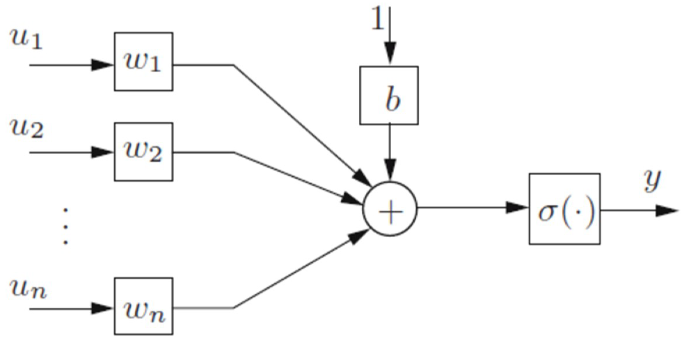
The second method used in our work is based on artificial neural networks (ANN). Their principles mirror the organization and mechanism of the human brain (10 billion neurons) based on learning and memory [31,32]. ANN are composed of a specified number of single processing units called neurons (See Figure 4).

The classical neuron model is described by (10).

$$y=\sigma \left({\displaystyle \sum }_{i=1}^n{w}_i{u}_i+b\right)$$

(10)

where $u_i \left(i = 1, 2,\dots , \mathrm{n}\right)$ denotes the neuron inputs, b is the bias (threshold), $w_i$ denotes the synaptic weight coefficients, σ is the nonlinear activation function such that sigmoid and hyperbolic tangent functions.

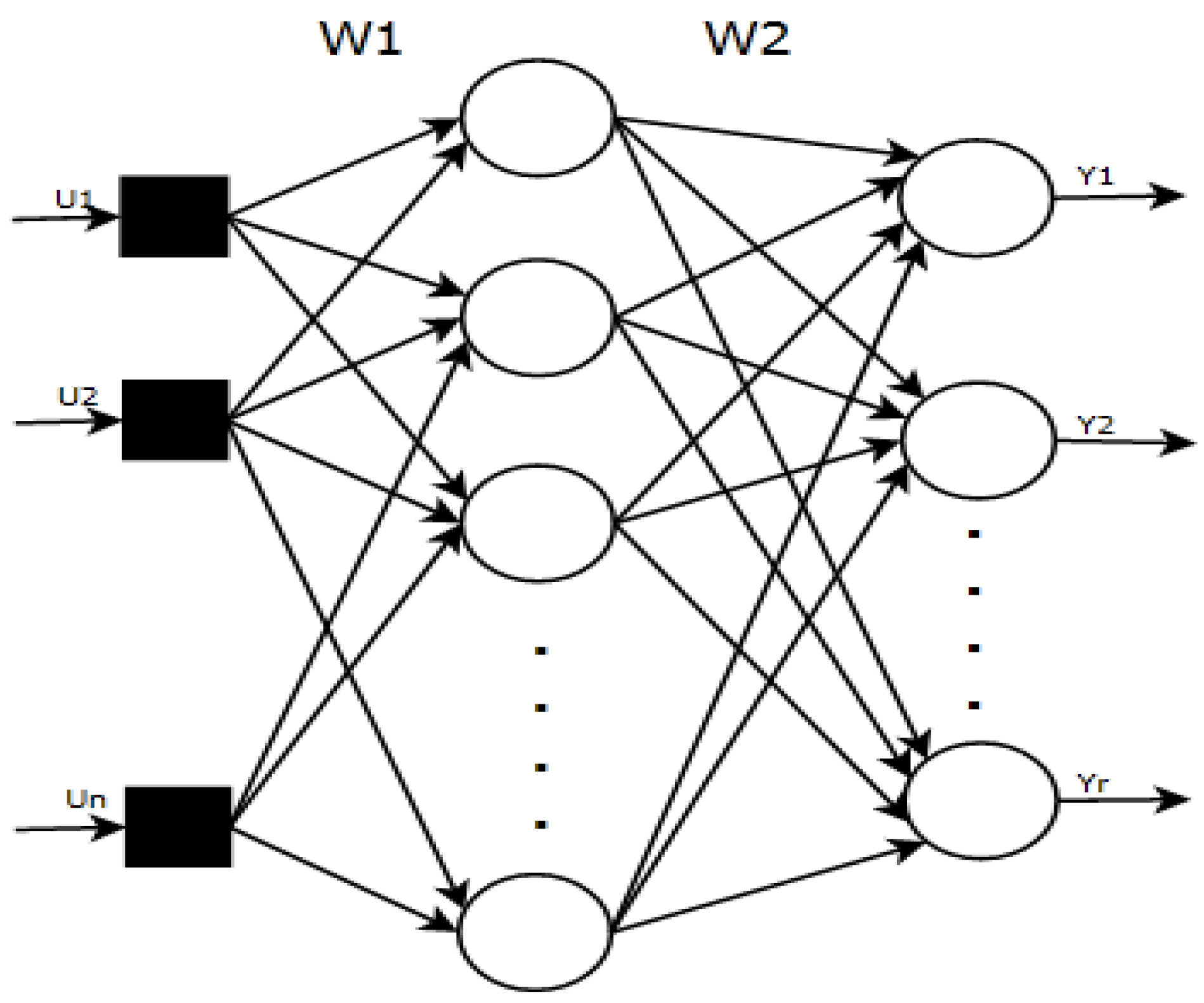
The multilayer neural network is a network in which the neurons are grouped into layers. Such a network has an input layer, one or more hidden layers, and an output layer (Figure 5). The fundamental neural data processing is carried out in hidden and output layers.

The neurons constituting each layer are linked to all the neurons of the following layer. For each connection, a weighting coefficient is assigned which is determined according to the tasks that should be solved by this neural network.

The output layer generates the network response vector $Y$. Non-linear neural computing performed by the network shown in (Figure 5) can be expressed by (11).

$$Y={\sigma }_2\left\{W_2{\sigma }_1\left(W_{1}U\right)\right\}$$

(11)

where:

• ${\sigma }_1$ and ${\sigma }_1$ are vector-valued activation functions which define neural signal transformation through the 1st and output layers;
• $W_1$ and $W_2$ are the matrices of weight coefficients which determine the intensity of connections between neurons in the neighboring layers;
• U, Y are the input and output vectors, respectively.

One of the fundamental advantages of neural networks is that they have the ability of learning and adapting. The training of a neural network is the determination of weight coefficient values between the neighboring processing units.

The Back-propagation (BP) is a popular feedforward multi-layered network learning algorithms. It optimizes the value of synaptic weights between neurons by minimizing the sum-squared error using the gradient descent method. The modification of the weights is performed according to the Formula (12).

$$W\left(k+1\right)=W\left(k\right)-\eta ∆J\left(W\left(k\right)\right)$$

(12)

where:

• $W\left(k\right)$ denotes the weight vector at the discrete time k,
• η is the learning rate,
• $J(W\left(k\right)$ is sum-squared error:

  $$J\left(W\left(k\right)\right)=\left|\right|d^k-y^k{\left|\right|}^2$$

  (13)

$y^k$ is the output vector and $d^k$ is the desired output vector.

The standard BP has proven its performance in practical applications. But the disadvantage of these methods requires fixing the architecture of the network before starting the learning phase. The diagnosis using the Back-Propagation Neural Network method will be seen in Section 4.2.

3.3. Genetic Algorithm based Neural Network

The first methods that have been implemented to avoid defining in advance the neural network architecture are based on the technique of the extension of geometry. These methods begin the training phase with a limited number of hidden layers and neurons and increase their numbers progressively. But they were used without reaching the optimal architecture [33,34,35].

In this article, we apply genetic algorithms for a dual purpose. Find both the ideal architecture of the neuron network (number of hidden layers) and the good values of the neural weights and thresholds. The principle of the approach is to assign to each layer, during the codification of chromosomes, a value between 0 and 1. The layer will only be activated if this value is greater than a threshold defined in advance (in our case at 0.3).

We will see in the following the general principles of genetic algorithms and how we combined them with neural networks.

GAs were created by analogy with natural phenomena. They simulate the natural evolution of organisms (individuals), generation after generation, respecting heredity phenomena during reproduction by crossover, mutation and replacement. In a population of individuals, these are the best adapted to the environment, who survive and give offspring. Such algorithms were developed in 1950 by biologists, and then these algorithms were adapted for the search of solutions of optimization problems [36,37,38,39].

The GAs are then based on the following phases:

• Initialization: An initial population of N chromosomes is randomly drawn.
• Evaluation: Each chromosome is decoded and evaluated.
• Selection: Creation of a new population of N chromosomes by the use of an appropriate selection method.
• Reproduction: Possibility of crossover and mutation within the new population.
• Return to the evaluation phase until the algorithm stops.

After briefly seen the principle of genetic algorithms, we will look closely how to implement it through the coding of individuals and the application of genetic operators.

3.3.1. Initial Population Codification:

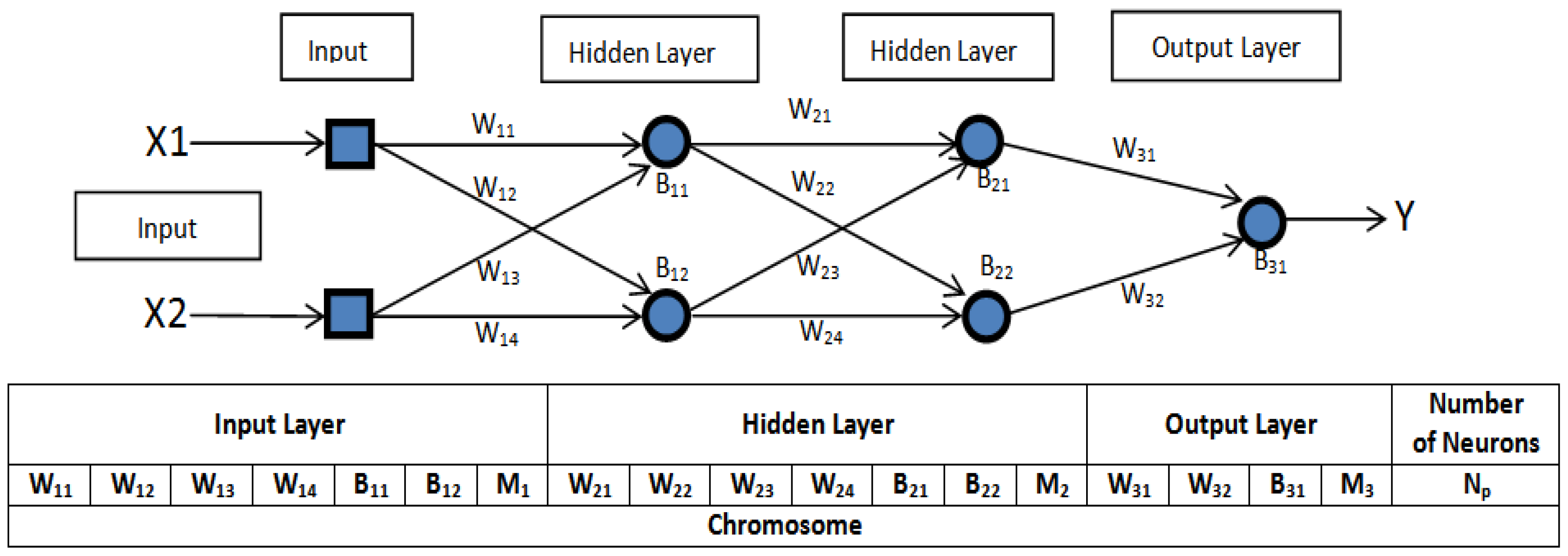
With regard to the coding of the elements of a population, it is necessary to represent the different individuals in a usable form for a GA. This form, called the chromosome, is composed of genes that correspond to the different parameters of the solution. In the case of our study, the solution corresponds to the optimal neural network which is coded in the form of a chromosome encompassing all the data necessary for its implementation.

The algorithm used in our research has the particularity of being able to find the optimal number of hidden layers ($N_l$) and the optimal number of neurons in each of these layers ($N_p$). The same number of neurons in each layer is fixed and it is equal to $N_p$. This method is an improved version of the one proposed by [40].

Let $W_i$ and $B_i$ respectively the matrices of weights and biases of each layer. (‘i’ is the layer number) To be able to codify neural networks with a constant length chromosome, we have added to each field coding a network layer “i” a number $M_i$. The layer will only be activated if the value of this field is greater than the threshold value $M_i$≥ 0.3. Regarding the number of neurons in each hidden layer ($N_p$), the code is added at the end of the chromosome.

As an example, consider a network with three layers of neurons with two inputs, two neurons in each hidden layers and one neuron in the output layer (Figure 6). We set the maximum number of layers to 3 and the maximum number of neurons in each layer to 2. The length of the chromosome is therefore 19.

3.3.2. Fitness Function

Whenever a new individual has been created, it must be associated with a value (called fitness or evaluation function) that measures the quality of the solution. This value will be used by selection processes to favor the best suited individuals who are the best solutions to the problem. Evaluation therefore represents the performance of the individual in relation to the problem to be solved.

In our case, we try to quantify the ability of an ANN to learn. The individual will have a fitness function value as low as it will be a good solution to the problem of optimization. We choose a fitness function $FF$ in our case that equals the Mean Squared Error expressed by (14) [41].

$$FF={\displaystyle \sum }_i{\left(d_i-a_i\right)}^2$$

(14)

$d_i$ and $a_i$ are the desired and calculated outputs of a ANN.

3.3.3. Selection Operator

A selection process is necessary to choose the chromosomes that ensure an improvement in the quality of the solutions. Selection is a process of choosing among all individuals in the population those who will participate in the construction of a new generation. This choice is essentially based on the values of the fitness function of each individual. A member with a low value of the fitness function will have a better chance of being selected to participate in the reproduction of the next generation.

There are different techniques to implement selection in Genetic Algorithms. In the case of our study, we chose the Tournament Selection. It consists of a meeting between several individuals randomly selected from the population. The winner of the tournament is the individual of better quality.

3.3.4. Crossover Operator

In general, crossover consists of applying procedures to selected individuals to reproduce one or more children who must inherit certain characteristics of the parents. This operator is used with a certain probability called the crossover rate ($P_C\in \left[0,1\right])$ which represents the proportion of the parent population that will be used for reproduction [42]. The most commonly used rates are in the range [0.45, 0.95].

We can mention some types of crossover operators as: One Point Crossover, Multi Point Crossover, Uniform Crossover, and Whole Arithmetic Recombination. In our case, we used a two-point crossover operator with a rate of 0.7.

3.3.5. Mutation Operator

A mutation can be defined as a small random adjustment in the chromosome, to obtain a new solution [43]. It is used to maintain and introduce diversity into the genetic population and is generally applied with low probability. If the probability is high, the GA is reduced to a random search. The mutation operator allows in other words the exploration of the entire research space. In the case of our study, the mutation operator is applied to 3% of the population at each generation.

3.3.6. Replacement Operator

This last step in the iterative process consists of incorporating new solutions into the current population. New solutions are added to the current population to replace partial old solutions. Generally, the best solutions replace the worst ones; this results in an improvement of the population [43].

Section 4.3 will be devoted to the bearing fault diagnosis by the use of this modified neural networks technique.

4. Vibration Fault Diagnosis

4.1. Linear Discriminant Analysis Based Fault Diagnosis

The purpose of the LDA is to automatically classify the bearings into one of the following 4 categories (Healthy Bearing, Inner Ring Fault, Ball Fault, Outer Ring Fault). For this purpose, we used the data obtained from the analysis of the 1044 available signals: Matrix of 1044 lines and 16 columns including 731 lines for learning and 313 lines for testing. For this model we used only learning and test data.

The global classification rate for training and test data has reached a F1-Score of 96.26% (

Table 1. Classification rate of LDA model (Training data).

		Predicted Class
		Healthy Bearing	Inner Ring Fault	Ball Fault	Outer Ring Fault	Recall
ActualClass	Healthy Bearing	119	0	0	1	99.17%
	Inner Ring Fault	0	196	2	2	98.00%
	Ball Fault	0	2	200	3	97.56%
	Outer Ring Fault	1	2	2	201	97.57%
	Precision	99.17%	98.00%	204%	97.10%

and

Table 2. Classification rate of LDA model (Test data).

		Predicted Class
		Healthy Bearing	Inner Ring Fault	Ball Fault	Outer Ring Fault	Recall
ActualClass	Healthy Bearing	57	0	1	2	95.00%
	Inner Ring Fault	0	85	2	1	96.59%
	Ball Fault	1	3	75	4	90.36%
	Outer Ring Fault	2	3	5	72	87.80%
	Precision	95.00%	93.41%	90.36%	91.14%

). For the test data it can be deduced that the best classification rate is obtained for the inner ring faults with a Recall value which is equal to 96.59% (85 faults from 88 that have been identified). The worst misclassification rate is recorded for outer ring faults with a rate of false discovery equal to 12.20% (10 faults among 82 have not been identified). The F1-score for the test data is equal to 92.33%.

The classification rate obtained by the LDA model remains insufficient for a model that is called to recognize defects on flying systems and whose consequences of a bad diagnosis can cause catastrophic results. Thus, to improve the obtained results, we extend our investigation with another more efficient diagnostic model. The model that will be used is based on Artificial Neural Networks.

4.2. Back-Propagation Neural Network Based Fault Diagnosis

The purpose of this subsection is to classify the bearings in the categories (Healthy bearing, Inner Ring Fault, Ball Fault, Outer Ring Fault) but with a better efficiency. The same database as above was used. It consists of 1044 lines corresponding to the number of signals and 16 columns corresponding to the descriptor extracted from the signal analysis. The data were subdivided as follows: 60% for Training (626 lines), 20% for validation (210 lines), and 20% for the test (210 lines).

We used a neural network with one hidden layer. The number of neurons in the input layer is 16 corresponding to the number of the descriptors. The Back-propagation algorithm has been tested to train the neural network.

The particularity of this network is that it contains 2 neurons in the output layer instead of 4. This choice allows decreasing the number of weights and consequently the calculation will be faster.

The neurons in the output layer will take values 1 or −1 depending on the desired classification decision. The set of possibilities is summarized in

Table 3. Output layer classification.

Fault	Output 1	Output 2
Healthy Bearing	1	1
Inner Ring Fault	−1	1
Ball Fault	1	−1
Outer Ring Fault	−1	−1

. We used the neural transfer function “tansig” to calculate the outputs of each layer.

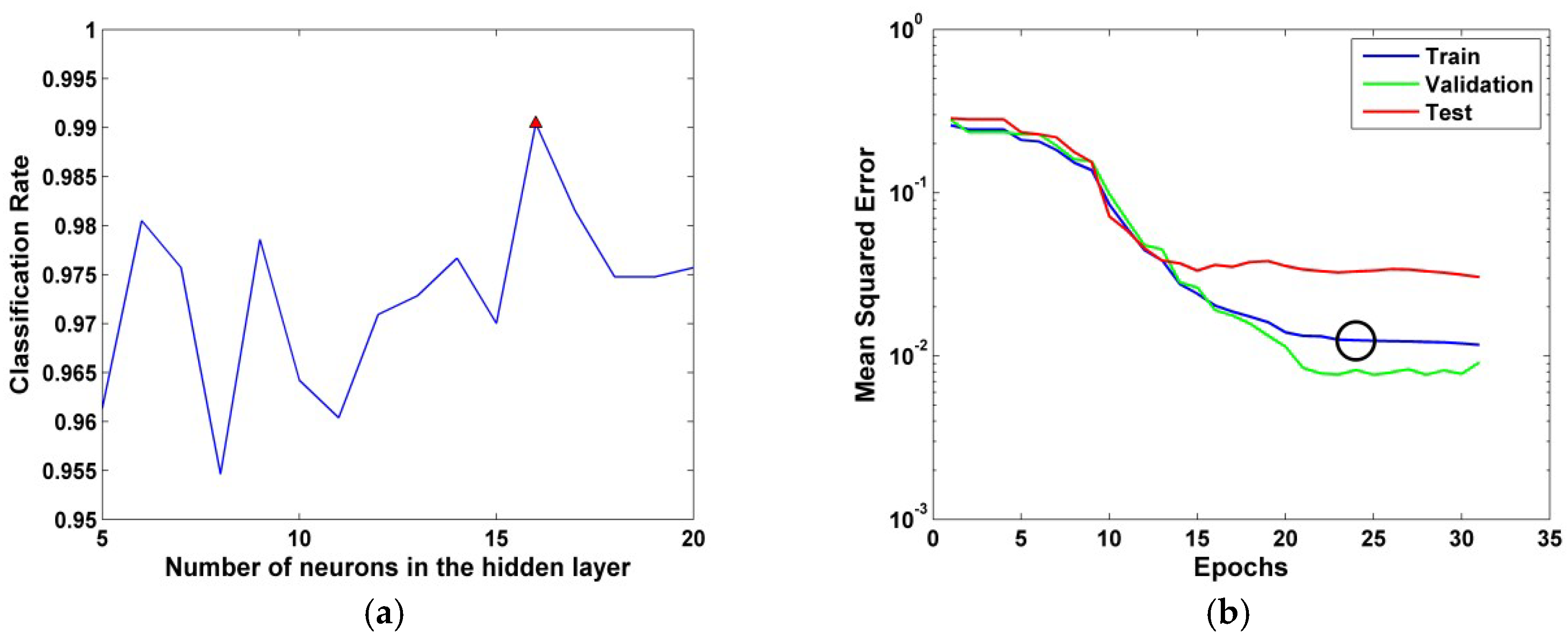
Several tests were performed by changing the number of neurons in the hidden layer each time. The optimal neural network is composed of 16 neurons in its hidden layer (Figure 7a). This network converged after 24epochs with Mean Squared Error MSE = 0.0124 (Figure 7b).

As noted above, the data were subdivided to 3 parts. For the training data the F1-Score obtained is 99.04%, the validation data the score is 97.62% and for the test data the score is 96.67% (

Table 4. Classification rate for Back-Propagation neural network (Training data).

		Predicted Class
		Healthy Bearing	Inner Ring Fault	Ball Fault	Outer Ring Fault	Recall
ActualClass	Healthy Bearing	98	0	0	0	100%
	Inner Ring Fault	0	177	0	1	99.44%
	Ball Fault	0	0	171	2	98.84%
	Outer Ring Fault	0	0	3	167	98.31%
	Precision	100%	100%	98.28%	98.31%

,

Table 5. Classification rate for Back-Propagation neural network (Validation data).

		Predicted Class
		Healthy Bearing	Inner Ring Fault	Ball Fault	Outer Ring Fault	Recall
ActualClass	Healthy Bearing	35	0	0	0	100%
	Inner Ring Fault	0	62	0	1	98.41%
	Ball Fault	0	0	57	2	96.61%
	Outer Ring Fault	0	1	1	51	96.23%
	Precision	100%	98.41%	98.28%	94.44%

and

Table 6. Classification rate for Back-Propagation neural network (Testing data).

		Predicted Class
		Healthy Bearing	Inner Ring Fault	Ball Fault	Outer Ring Fault	Recall
ActualClass	Healthy Bearing	47	0	0	0	100%
	Inner Ring Fault	0	47	0	1	97.92%
	Ball Fault	0	0	53	3	94.64%
	Outer Ring Fault	0	1	2	56	94.92%
	Precision	100%	97.92%	96.36%	93.33%

). It can be seen from the test data that among the 56 cases of ball faults bearing, 3 were misclassified with a rate of false discovery is equal to 5.36%. Regarding the 59 defects of the outer ring, 3 of them were not well predicted. The rate of false discovery is equal to 5.08%.

The tests show a classification rate improvement compared to the LDA method. These results are obtained with a network having 16 neurons in a single hidden layer.

The disadvantage of this approach is that we made several tests by changing each time the number of hidden layers and the number of neurons without being sure to reach the optimal value. To achieve this goal, we have chosen genetic algorithms as a method of optimizing the neural network.

4.3. Cooperative GA-Neural Network Based Fault Diagnosis

Like the two methods previously used, we used the same database with the same repartition of data (626 lines for training, 210 for validation and 210 for testing). We have kept the same goal which is classifying bearings in the four categories mentioned in previous chapters.

As indicated in Section 3.3, we will use modified artificial neural networks to achieve this goal. The number of maximal hidden layers and neurons are respectively set at N_l = 5 and N_p = 20. This choice is largely sufficient to build this network.

The optimization method we adopted allowed us to determine not only the structure of the neural network (number of hidden layers and neurons) but also the weights and thresholds values of neurons. According to the coding method adopted, the length of the chromosome will not depend on the architecture of the neural network but only on the maximum numbers of hidden layers and neurons that have been fixed in advance (N_l and N_p). This length is equal to 2069 divided according at the

Table 7. Chromosome codification length.

Input Layer			Hidden Layer			Output Layer			Length of Number of Neurons Code
Weights	Bias	Activation Threshold	Weights	Bias	Activation Threshold	Weights	Bias	Activation Threshold
320	20	1	1600	80	4	40	02	1	1

.

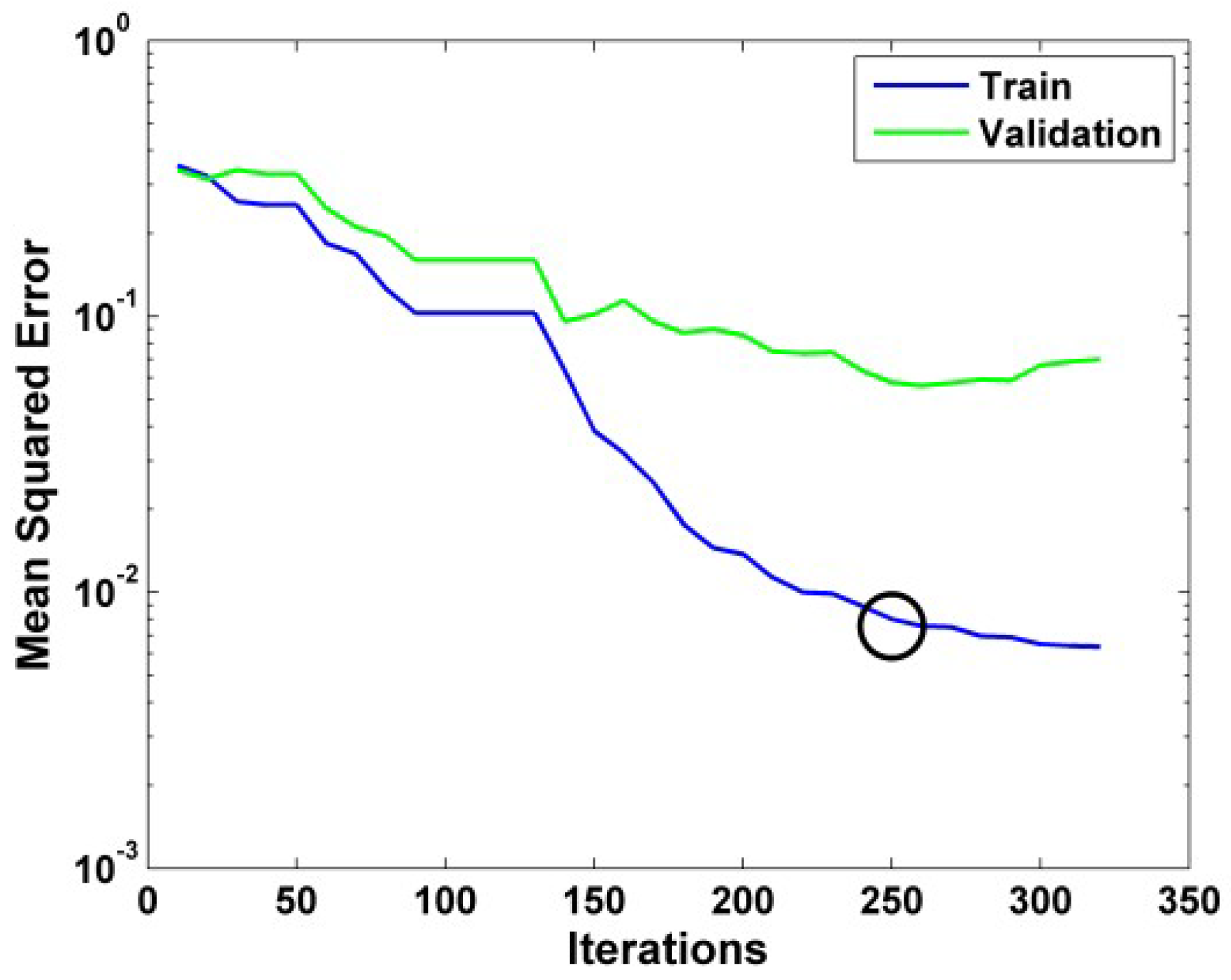
The best performances were obtained by gradually increasing the population size and the number of iteration. The Best global GA parameters are shown in

Table 8. Genetic Algorithm Parameters.

Population Size	100	Crossover Percentage (Pc)	0.7
Numberof Max Iteration	1000	Mutation Percentage (Pm)	0.3

. This optimization allows us to retain the optimal network that consists of 3 hidden layers and 13 neurons in each layer. The algorithm has converged after 25 iteration with Mean Squared Error MSE = 0.076 (Figure 8).

The classification results obtained by this model are as follows: For learning data, the F1-Score is 100% and for validation and test data, the scores are respectively 99.14% and 99.12%. From the test data we can deduce that only one ball bearing defect on 55 has not been identified and only one outer ring bearing fault on 53 has not been identified. For healthy bearings and bearings with inner ring defects, the classification rate is 100% (

Table 9. Classification rate for Cooperative GA-neural network based Fault Diagnosis (Training data).

		Predicted Class
		Healthy Bearing	Inner Ring Fault	Ball Fault	Outer Ring Fault	Recall
ActualClass	Healthy Bearing	113	0	0	0	100%
	Inner Ring Fault	0	163	0	0	100%
	Ball Fault	0	0	179	0	100%
	Outer Ring Fault	0	0	0	171	100%
	Precision	100%	100%	100%	100%

,

Table 10. Classification rate for Cooperative GA- neural network based Fault Diagnosis (Validation data).

		Predicted Class
		Healthy Bearing	Inner Ring Fault	Ball Fault	Outer Ring Fault	Recall
ActualClass	Healthy Bearing	33	0	0	0	100%
	Inner Ring Fault	0	59	0	0	100%
	Ball Fault	0	0	53	1	98.15%
	Outer Ring Fault	0	0	1	62	98.41%
	Precision	100%	100%	98.15%	98.41%

and

Table 11. Classification rate for Cooperative GA- neural network based Fault Diagnosis (Test data).

		Predicted Class
		Healthy Bearing	Inner Ring Fault	Ball Fault	Outer Ring Fault	Recall
ActualClass	Healthy Bearing	34	0	0	0	100%
	Inner Ring Fault	0	66	0	0	100%
	Ball Fault	0	0	54	1	98.18%
	Outer Ring Fault	0	1	0	53	98.15%
	Precision	100%	98.51%	100%	98.15%

).

Compared to the LDA and the classical ANN classifiers, the Neural Network based model optimized with Genetic Algorithms was more effective in classifying vibration bearings defects. These results have been validated by test data with a F1-Score of 99.12%. The global score for training, validation and testing data is 99.65%. These results are obtained thanks to this approach which has the capacity to optimize the architecture of the neural network.

All experiments were performed with Matlab R2017b software on a machine having the following characteristics: Intel Core i5 2.4 GHz processor with 4.0 GB of RAM. The execution time of the algorithm is 13 min 15.03 s.

It should be noted that this time which has been calculated is not the diagnosis time, but the time which is necessary for the optimization and the learning of the neural network. This operation is carried out only once to build the model.

In addition to its ability to accurately classify defects, this method provides a quick diagnosis for making decisions in time. This ability is very useful for flight systems which require a high operational safety. This model is validated to ensure an automatic diagnosis of the vibration defects of the aircraft air compressor bearings.

5. Conclusions

In this paper, we present an approach to diagnose vibratory failures of a bearing mounted on an aircraft air compressor. Vibratory signals were acquired on the test bench at the front bearing housing. The Welch spectral power estimate was used efficiently to analyze these signals and extract the characteristic frequencies. The data obtained are grouped into 4 classes (Healthy Bearing, Inner race fault, Ball fault, Outer race fault) and they were used for learning two fault monitoring models.

The first method used is Linear Discriminant Analysis; its classification rate remains insufficient in our case study.

Regarding the second method, the Feed Forward neural network has been tested with the Back-Propagation algorithm for training. Compared to the LDA method, the results have been improved without attaining the maximum rate of classification.

Regarding the third method, we have opted for genetic algorithms to find the optimal neural network architecture to improve classification performance. The classification rate has reached a F1-Score of 99.65. Thus, this model has been validated for the diagnosis of vibratory defects of bearings.

The contribution of this work is to set up a method of diagnosis of vibratory defects based on a modified version of the neural networks. The optimization of ANN by Genetic Algorithms has significantly improved the classification performance of bearing faults.

Moreover, this method is characterized by rapid diagnostic decision making and ease of implementation on ground-based computers or in-flight systems. Its advantage lies in its ability to know the state of the rolling elements without disassembling the turbojets.