Effective Prediction of Bearing Fault Degradation under Different Crack Sizes Using a Deep Neural Network


1
School of IT Convergence, University of Ulsan, Ulsan 44610, Korea
2
School of Electronics and Computer Engineering, Chonnam National University, Gwangju 61186, Korea
*
Author to whom correspondence should be addressed.
Appl. Sci. 2018, 8(11), 2332; https://doi.org/10.3390/app8112332
Submission received: 24 October 2018
/
Revised: 12 November 2018
/
Accepted: 19 November 2018
/
Published: 21 November 2018
(This article belongs to the Special Issue Fault Detection and Diagnosis in Mechatronics Systems)
Abstract
:Exact evaluation of the degradation levels in bearing defects is one of the most essential works in bearing condition monitoring. This paper proposed an efficient evaluation method using a deep neural network (DNN) for correct prediction of degradation levels of bearings under different crack size conditions. An envelope technique was first used to capture the characteristic fault frequencies from acoustic emission (AE) signals of bearing defects. Accordingly, a health-related indicator (HI) calculation was performed on the collected envelope power spectrum (EPS) signals using a Gaussian window method to estimate the fault severities of bearings that served as an appropriate dataset for DNN training. The proposed DNN was then trained for effective prediction of bearing degradation using the Adam optimization-based backpropagation algorithm, in which the synaptic weights were optimally initialized by the Xavier initialization method. The effectiveness of the proposed degradation prediction approach was evaluated through different crack size experiments (3, 6, and 12 mm) of bearing faults.
1. Introduction
Rotary machines are the most important constituents in industrial production due to their popularity, reliability, and economic benefits. However, unexpected failures of these machines can cause unanticipated interruptions, sudden breakdowns, and economic losses in industrial production. In rotary machines, the rolling bearing elements are the components most responsible for making systems operations flexible and smooth. Bearings are ubiquitous components and billions of these are used in different machines operating under different conditions. Unfortunately, bearing-related faults account for many mechanical failures due to frequent contamination from working environment conditions and other influences such as overloading or misalignment in assembly. About 50% of bearing faults are related to bearing defects [1,2]. Consequently, the unexpected failure of bearings is the fundamental cause of sudden mechanical interruptions in industry, leading to heavy economic losses and even to catastrophic consequences, especially in critical systems [3,4]. Hence, the correct detection and prediction of bearing fault severity at an early stage of bearing lifetime is urgently needed for dependable bearing condition monitoring and period maintenance decision of rotary machines in industry.
Some outstanding signal processing technologies have been extensively used to extract the characteristic fault frequencies from obtained bearing data for an effective incipient fault detection in critical mechanical systems [5,6,7,8]. The envelope analysis method is an effective technique to extract the low-frequency fault components from the high-frequency carrier signal recording bearing conditions [4,6]. One of the main advantages of using envelope analysis is the fact that it is more robust to different sorts of noises that may affect the raw signal of bearings. If we directly process this raw data, then even minor sources of noise cause a huge problem resulting in decreasing the fault detection performance. Furthermore, power spectrum estimation approaches have also been widely studied in [9,10], which employ the multivariate divergence calculation techniques to effectively approximate signal power spectrum density. However, construction of an appropriate spectrum estimation model for evaluating bearing degradation still remains a significant challenge. Otherwise, condition monitoring systems usually collect a massive amount of data after machines have been operating for a long time, resulting in the instant requirement of intelligent processing solutions that can efficiently analyze the data and provide a highly accurate result [11]. Moreover, the advent of cloud computing and the internet is set to usher in the era of mechanical big data. With more and more data available to us, it is essential to use intelligent learning models that can extract useful information from the measured data for fault detection and diagnosis. The developed techniques based on machine learning [12,13] and deep learning [14,15,16] have generally been applied in estimating the defect severity of bearings and in diagnosing those defects under varying conditions. These approaches are an effective solution for big data analytics, which are common nowadays [17,18,19,20,21].
Based on deep learning methods, this paper proposes an efficient comprehensive methodology for correct prediction of fault degradation levels of bearings under different crack size conditions using the signal envelope spectrum analysis technique and deep neural network (DNN). Envelope analysis is an effective signal demodulation technique which exactly detects abnormal symptoms to obtain the bearing defect signal. Afterward, a Gaussian window method is exploited only to accurately capture the characteristic fault frequencies from the envelope spectrum domain, in which a health-related indicator (HI) is first measured by computing the ratio of defect spectrum components to original spectrum components for estimating the fault severity of bearings. These HI values are learning databases for DNN training. In this work, a proposed DNN was trained to predict the degradation levels of bearings based on the original envelope power spectrum (EPS) at the input of the neural network. The DNN training processing was performed using the Adam optimization-based backpropagation algorithm, which supplies fast learning speed and high accuracy. Moreover, a Xavier initialization method was also proposed to optimally set the synaptic weights and biases of neural networks that enhance convergence of the DNN. The methodology proposed in this paper was expected to yield higher performance than the existing methods.
The remaining sections of this paper are organized as follows. Section 2 describes an experimental system for bearing data acquisition. Section 3 presents a proposed comprehensive methodology for effective prediction of bearing degradation levels, and Section 4 presents and discusses the achieved results. Finally, the conclusion is given in Section 5.
2. Fault Data Acquisition System
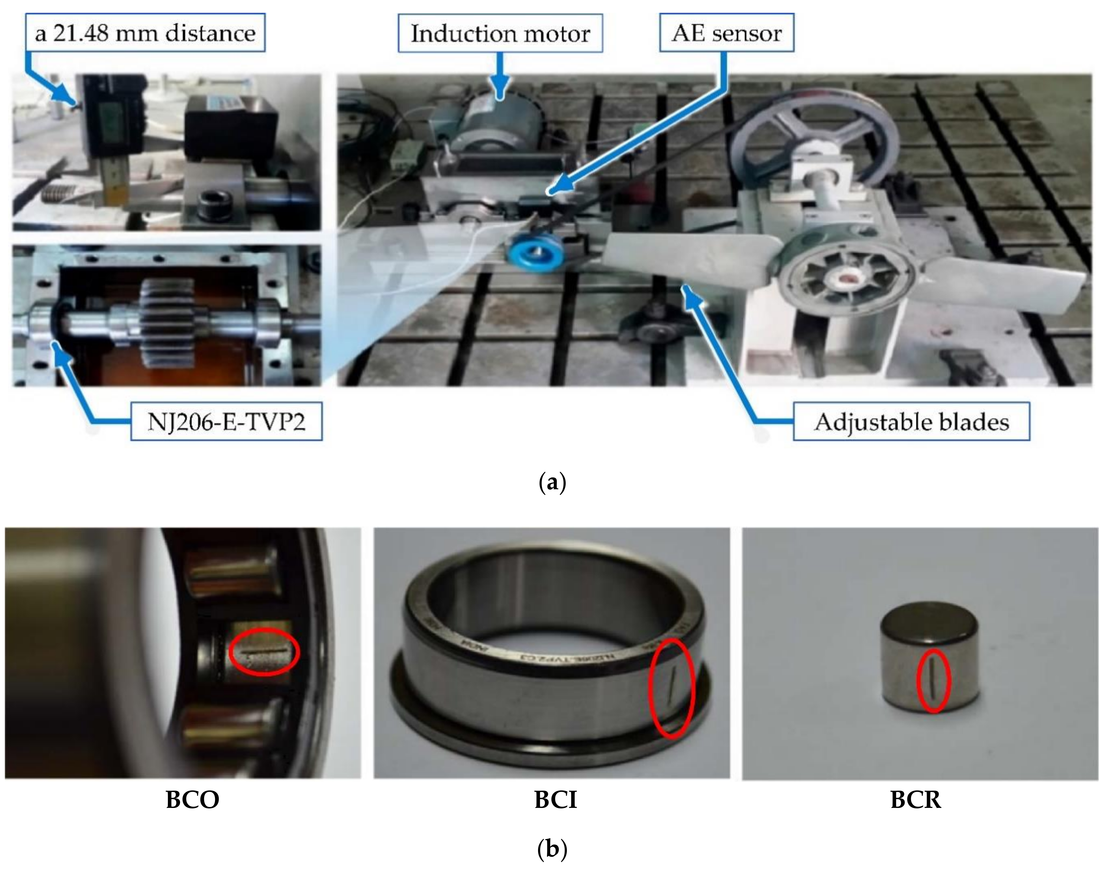
An experimental system of bearing fault simulation in machinery is illustrated in Figure 1a. This experimental model for bearing condition acquisition has been widely used in previous research and has supplied satisfactory performance in bearing fault detection and diagnosis. Basically, the system setup consists of two driven and nondriven end shafts, which are linked together via a gearbox on the inside and fastened on the framework using NJ206-E-TVP2 bearings. The nondriven end shaft is loaded by two adjustable blades connected using a pulley and belt.
An acoustic emission (AE) sensor with a wideband operation is attached on top of the nondriven end bearing housing at a 21.48-mm distance to capture the continuous information of bearing conditions in the time domain. This AE sensor is directly connected to a PCI-2 based data acquisition system to digitize the signals for further processing. In this study, AE signals of bearing conditions were acquired for a duration of 5 s and a sampling frequency of 250 KHz. The bearings used for condition monitoring were seeded with three primary defect types generated at various positions on the bearing’s surface, consisting of a bearing crack on the outer surface (BCO), a bearing crack on the inner surface (BCI), and a bearing crack on the roller (BCR), as shown in Figure 1b. The bearing characteristic defect frequencies were computed and are described in Table 1. They included a ball pass frequency of the outer surface (BPFO), a ball pass frequency of the inner surface (BPFI), and two times of ball spin frequency (2 × BSF (ball spin frequency)). Mathematical formulas for calculating these characteristic frequency components are given particularly in [22]. In this work, the AE data of bearing defects were obtained under different crack size conditions (i.e., 3, 6, and 12 mm) for experimental verification.
3. The Proposed Methodology for Prediction of Bearing Defect Degradation Using Deep Neural Network
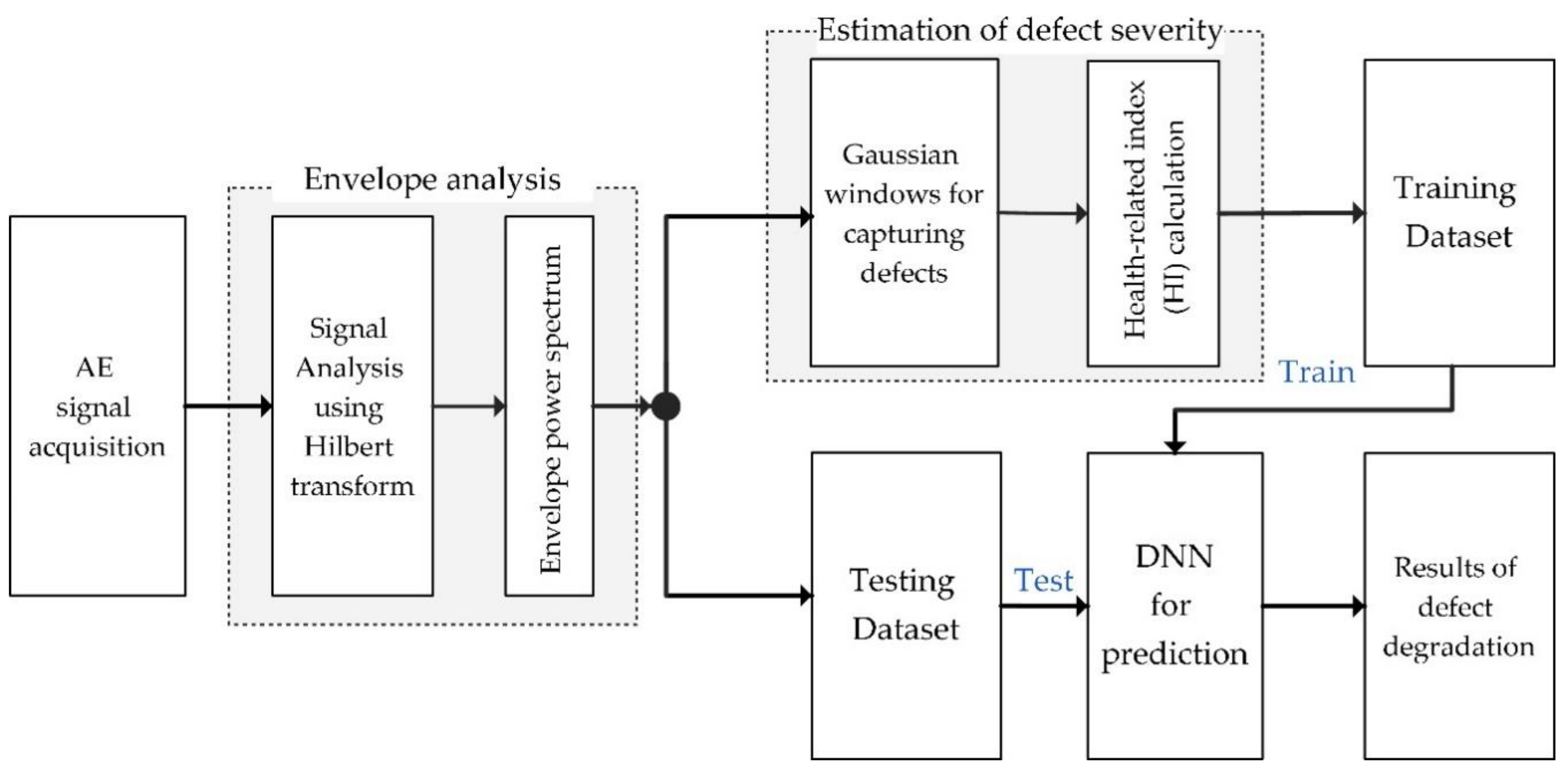
The comprehensive methodology for effective prediction of defect degradation in bearings under different crack size conditions consisted of two main steps: first, a Gaussian distribution model (GDM)-based window was set up for the envelope power spectrum (EPS) calculation to estimate the defect severity, then a DNN-based method was performed to effectively predict the fault severity of a series of defect degradations in bearings, as shown in Figure 2.
3.1. Estimation of Bearing Defect Severity Using the Gaussian Window Method
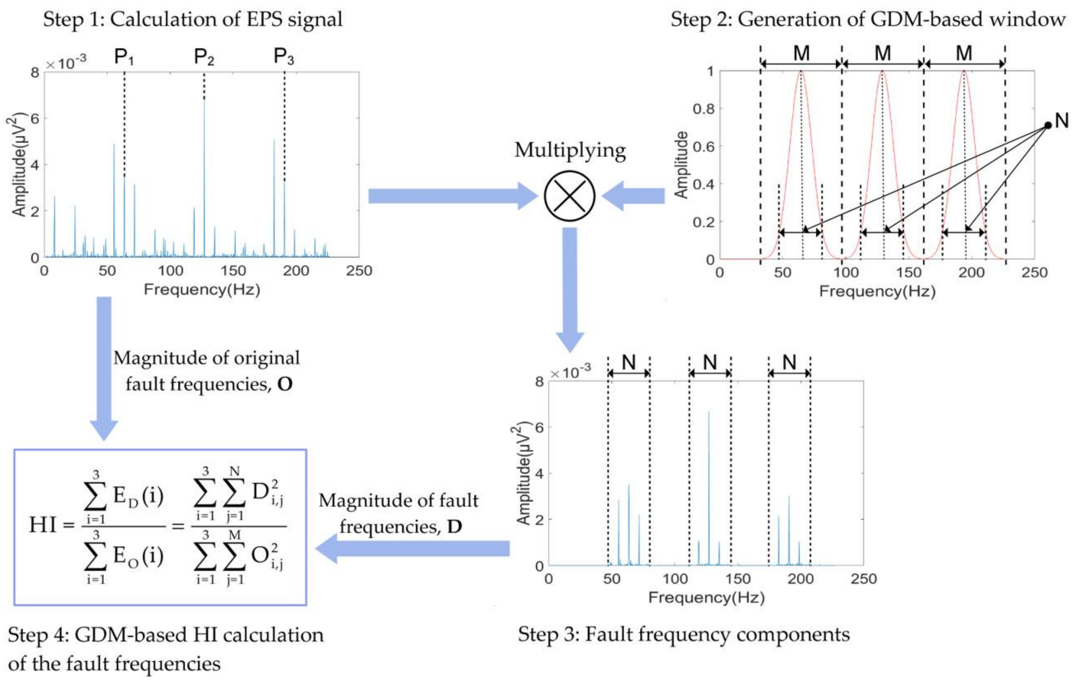
Through the observation of the abnormal symptoms at the harmonic frequencies of BPFO, BPFI, and 2 × BSF, an optimal approach for evaluating the defect severity of bearings was applied to correctly measure the defective degree, which was computed by using the GDM-based window method around harmonics of the fault frequencies, respectively. This GDM-based method has been extensively used for HI calculation to estimate the defect severity of bearings [8] and results in detecting and diagnosing the bearing defects. Figure 3 describes the process of estimating fault severity based on the Gaussian window method.
Step 1: The recorded AE signals related to the bearing conditions were processed by envelope analysis technique to detect the characteristic defect frequency components showing the abnormal symptoms in signal. The EPS signals were first calculated using the Hilbert transform [23] and delivered by the following equations:
where is the Hilbert transform of the time signal x(t), z(t) is the analytical signal, and the the envelope signal is illustrated by . The EPS signal was then determined by calculating the absolute value square of the fast Fourier transform (FFT) of the envelope signal, .
Step 2: A GDM-based window was used to catch the bearing fault frequencies and other around harmonics from their envelope spectrum domain. The values of the window were then determined as follows:
where is a parameter of Gaussian distribution, indicates the ith harmonic of the bearing defect frequencies, is an index term of each frequency bin, and represents the frequency bins around each defect frequency harmonic. In this study, was given for the outer surface, whereas or were defined for the inner surface and roller. Hence, the Gaussian windows for capturing the fault frequencies had a bell shape because of the appearance of the sidebands around the defect harmonics in their spectrum analysis domain.
Step 3: The original EPS signals were filtered by multiplying the GDM-based window values to select only the characteristic fault frequency components around the harmonics of bearing defect frequencies and to remove the redundant components in their spectrum signals, as presented in step 3 of Figure 3.
Step 4: After properly capturing the characteristic fault frequencies in step 3, a GDM window-based HI was calculated, as shown in Equation (5), which was based on measuring the energy of the defect frequency component to estimate the defect severity of bearings:
where is the amplitude of the frequency bin around the harmonic of the fault frequencies from the original signal spectrum domain, the corresponding energy defined by , is the amplitude of the frequency bin around the harmonic of the defect frequencies clearly obtained from the defective spectrum domain, and the corresponding energy defined by , and is the number of frequency bins exactly containing the defects. The HI calculation was performed in the range from 0 to 1 (i.e., 0 ≤ HI ≤ 1), which was suitable for DNN training in further processing, as given in step 4 of Figure 3.
3.2. DNN for Defect Degradation Prediction
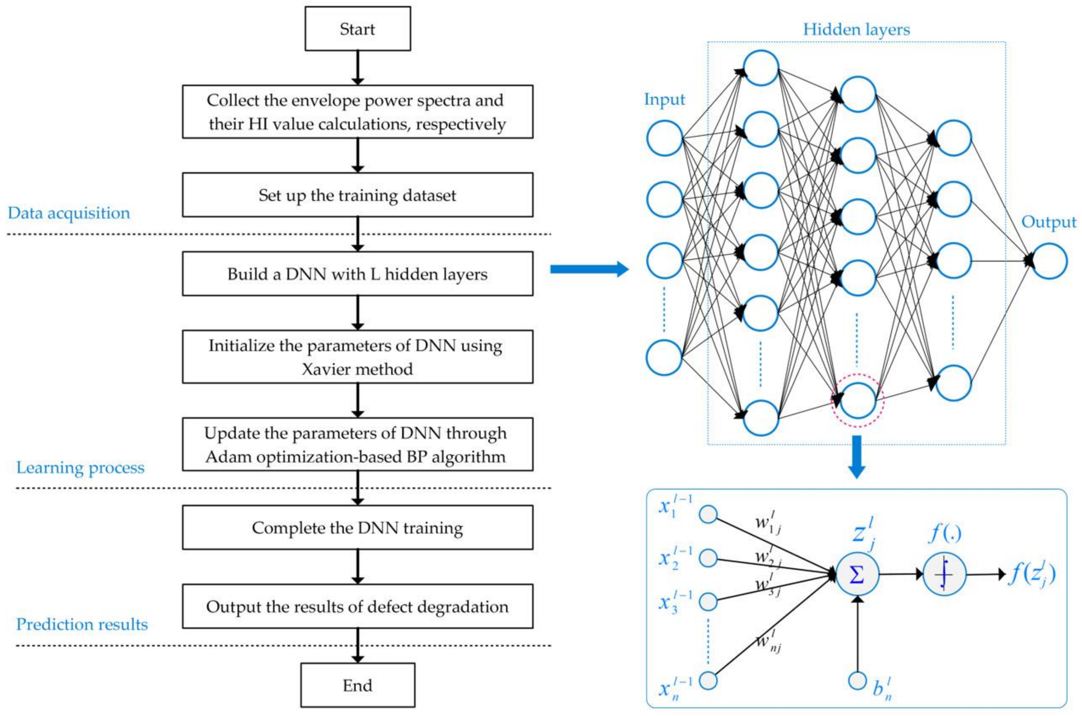
A deep learning technique was firstly applied for image classification [24], which was utilized to minimize the dimensionality of data representation and recognize targets effectively. For outstanding learning capability, the deep learning method has also been used successfully for image enhancement [25], in which a deep convolution neural network was presented to improve the contrast of low-quality images collected from under- or overexposed images. Consequently, a DNN can be trained to learn useful feature information directly from a dataset without requiring expert knowledge in the specified fields. In this paper, the proposed effective DNN-based method for predicting bearing fault degradation levels included three procedures: data acquisition of bearing defects under different crack size conditions, a learning process for DNN training, and evaluation of predicted results of bearing degradation levels, as illustrated in Figure 4. The DNN training process is thoroughly presented in the following sections.
DNN is a stacked layer model in which the layers are connected together and there are no connections of nodes within the same layer [16]. A DNN includes an input layer, an output layer, and a few hidden layers placed between them in the model. The number of nodes of an input layer is set corresponding to the dimensionality of the input data. Similarly, the number of nodes of an output layer is defined corresponding to the dimensionality of the target data. The number of nodes of every hidden neural layer is set in accordance with the network function, for which there are no required strict regulations. Each node in the next layer is directly linked to all nodes in the previous layer. Nodes of the first layer receive the input data and transmit them to other layers, while nodes of the last layer output the targets. The nonlinear relationship between the DNN layers is indicated by the following equations:
where is the activation value of neuron in layer ; is a linear activation combination of neurons in the previous layer; is the bias value of neuron in layer ; is the weight parameter between nodes in layer and in layer ; and is the activation function, which is usually chosen to be sigmoidal of the form and mostly used in DNN. Given the fixed setting of the model parameters to our data, a nonlinear form of hypotheses denoted the output of the neural network, which gave us a real number. The network outputs were serially calculated layer by layer on the model’s parameters, which were initialized appropriately.
3.3. Adam Optimization-Based Backpropagation Algorithm and Xavier Weight Initialization
To train the network, it is necessary to gain optimal operation parameters in DNN. In this study, the backpropagation algorithm was a good choice owing to the fact that it is a common method of training artificial neural networks used in conjunction with an Adam optimization method [26]. Backpropagation calculates the gradient of a loss function with respect to all the weights in the network. Suppose we have a fixed training set of training datasets. Then, the output target of the is . In detail, the loss function with the model’s parameters can be defined by calculating the mean square error (MSE), as in the following equation:
where J(W,b) is the loss function, M is the number of training dataset samples, is the target sample, and is the output sample of the neural network. Calculation of the loss function using MSE is simple and effective for linear regression problems.
In this paper, the loss function for estimating the undesired error ratio was calculated by average squaring the reconstruction error term, as given in Equation (8), which is widely used in measuring the difference between predicted and actual values. The main objective of DNN training is to minimize this loss function, making the error of the DNN outputs close or equal to zero. Hence, an Adam optimization algorithm was utilized and the pseudocode of method was given as
- ▪
- Set the learning rate: exponential decay rates for the moment: the loss function with the model’s parameters .
- ▪
- Start at time step : initialization of , 1st moment , and 2nd moment .While do not converge, do: calculating gradient of the loss function at: updating the first moment estimation: updating the second moment estimation: calculating the bias-corrected first moment: calculating the bias-corrected second moment.Update the parameters:end while, return .
Adam optimization is derived from adaptive moment estimation. This algorithm works better in practice compared to other learning methods due to its fast convergence that makes the learning speed of a model quite fast and efficient. The key step is computing the first and second moments of the gradients above. Backpropagation is a popular technique for neural network training, which gives an efficient way to compute these moments. We first propagated forward calculating the activations for all layers up to the output layer using the equations defining the forward propagation steps. Then, we propagated backward in the network carrying the squared error terms and updating the values using the Adam algorithm, in which we computed the first and second moments of the gradients of the loss function with respect to the model’s parameters and updated their values in the descent direction of the gradient to obtain the loss function minimum. Once the moments of the gradient were calculated, the DNN parameters were updated as follows:
Thus, to approximate properly the output targets, the backpropagation algorithm was used to minimize the undesired error at output via a loss function by adjusting the model’s parameters on the backward procedure of DNN. The process of calculating the gradient of a loss function and updating the model’s parameters was performed in a DNN training epoch. Training and adjusting the network parameters were an over and over again process until the error ratio of the DNN outputs had reduced to the minimum values.
The synaptic weights of a DNN are usually initialized random values and its biases are set to zero. A proper initialization of the weights in a neural network is critical to its convergence. If these weights are set too small, the variance of the input data starts to diminish as it goes through each layer of the neuron network. Hence, the input finally falls to a very low value that can be no longer useful. If the weights are set too large, the variance of input data has a tendency to rapidly increase after passing each layer. Consequently, the input gets so large that it also becomes useless. Because the nonlinear activation function might saturate for larger values, the network activations become saturated. As a result, random initialization does poorly with DNN.
Actually, the assignment of the initial network weights is usually a random process for DNN training because nothing is known about the data and how to assign the weights that are suitable for the particular cases. An appropriate initialization of the weights is very important for a neural network to function properly. Thus, we made certain that the weights were set in a reasonable value range. Xavier initialization is derived from the idea of keeping the input and output of a layer with the same variance and the zero mean [27]. Supposing a neuron layer and its variance (Var) are considered as
when each signal passes through a layer, we want to keep the same variance. Assume that the inputs and weights are independent and identically distributed Gaussians of zero mean, to obtain
The above equation shows that the variance of the output is the variance of the input but scaled by . To keep the variance of the input and output unchanged, set , which results in . Hence, we have arrived at the final Xavier initialization formula. The weights should be initialized using Gaussian distributions with a zero mean and a variance of , where denotes the number of neurons in a layer. This method works extremely well in many cases that are extensively used in the initialization of neural networks.
4. Experimental Results
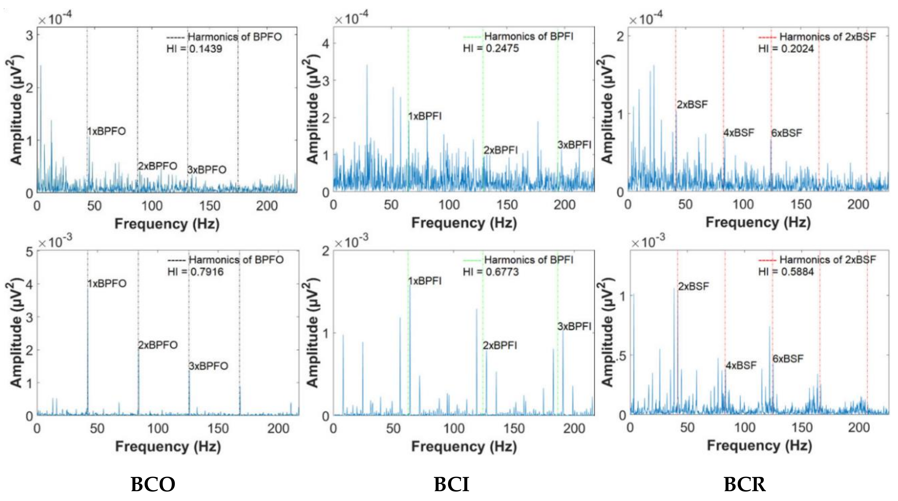
In this section, the authors present and discuss the achieved results of proposed research. The capability of the proposed DNN was evaluated through experimental results predicting the bearing degradation levels in the fault conditions of BCO, BCI, and BCR, which were collected under different crack size conditions. The 5-s AE signals of each bearing defect related to variable crack sizes were acquired at the sampling frequency of 250 KHz. Consequently, three datasets of bearings were given to verify the performance of the proposed approach. The detailed description of these datasets is given in Table 1. Each dataset contained 90 samples for each bearing health condition considered in this work. With three varying crack sizes of 3, 6, and 12 mm, there were 270 samples of each bearing condition collected for evaluation of degradation levels. Firstly, the EPS signals of bearing defects were calculated using the envelope analysis technique to detect the abnormal frequencies of bearings from the obtained spectral signals. A GDM-based window method was effectively applied only to capture the fault frequencies of BPFO, BPFI, and 2 × BSF in bearings for correct estimation of the fault severity via the HI computations. These obtained HI values for each bearing condition were the first training dataset for teaching the DNN to precisely predict the bearing degradation levels under the varying conditions used in this study. Figure 5 presents the obtained EPS signals of the bearing defects at different crack sizes and the correlated HI values representing the severity of those defects. The analysis results show that as the crack sizes generated in bearings became larger, the protrusion of periodic impulses around the harmonics at the characteristic defect frequencies became clearer, resulting in increasing HI values.
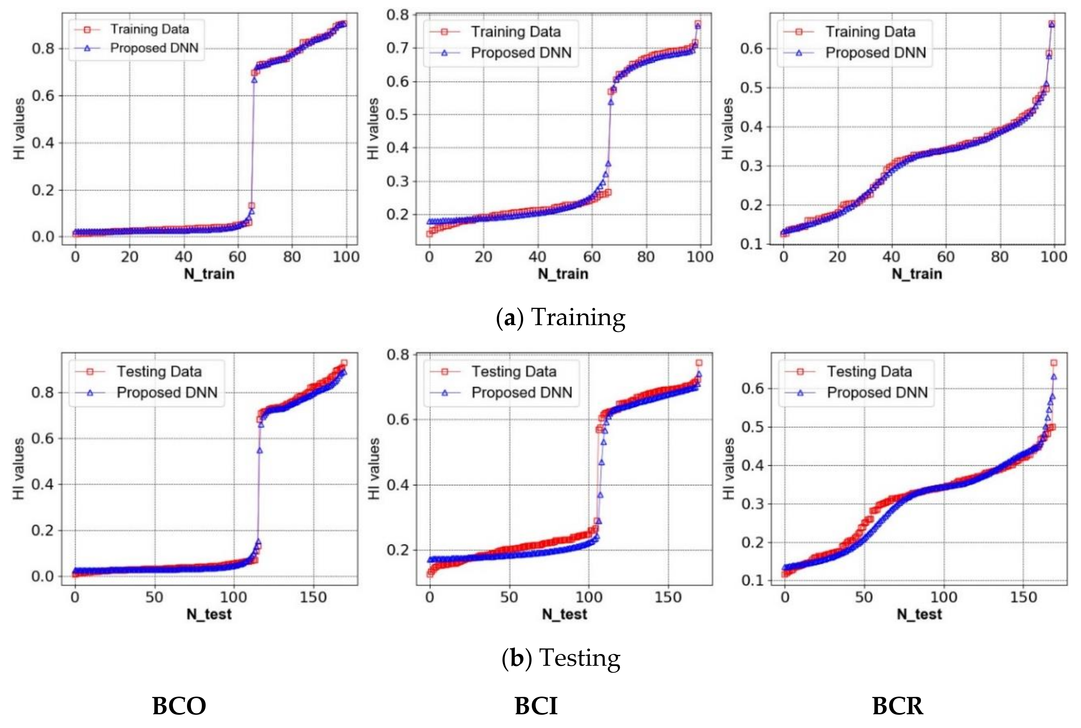
The proposed DNN was designed with five layers of neural networks consisting of one input layer, three hidden layers, and one output layer. The number of nodes in the input layer was determined based on the dimension of the input signal samples, and the number of nodes in the hidden layers were 800, 200, and 100, respectively. The output layer, however, was only one single node, which gave us the degradation levels of bearing defect conditions, as displayed in Figure 4. The neural layers of the proposed DNN used a sigmoidal function for activation. The synaptic weights and biases of the DNN were optimally initialized by the Xavier initialization method. The proposed DNN was trained using the Adam optimization-based backpropagation algorithm. The number of training iterations was set to 1000. This DNN was implemented using TensorFlow framework. As mentioned above, the dataset included three primary bearing defect conditions (BCO, BCI, and BCR) which were collected under three different crack sizes (3, 6, and 12 mm) for evaluation. Furthermore, the appropriate configuration of training and testing datasets was an essential aspect for evaluating DNN performance. In this study, 100 signal samples were selected randomly for training the DNN, and the remaining 170 signal samples were used to test the performance of the DNN. The number of training samples was kept less than the number of testing samples to ensure the high reliability of the prediction performance of the proposed DNN method. Each signal sample contained 2500 data points in the envelope spectrum analysis domain. The training and testing processes were accomplished for each bearing health condition, respectively. The prediction results of the bearing degradation using the proposed DNN method are shown in Figure 6, demonstrating that the proposed approach was able to efficiently predict the degradation levels of each bearing defect under varying crack size conditions.
In this work, to validate the effectiveness of the proposed DNN methodology in predicting the degradation levels of each bearing defect, the prediction accuracy (PA) was determined by the average absolute percentage error calculation, which is one of the most popular measures for prediction models [28]. This PA is computed as follows:
where Ai and Pi are the actual estimated and predicted values, respectively, and N is the number of data samples (i.e., Ntrain = 100, and Ntest = 170).
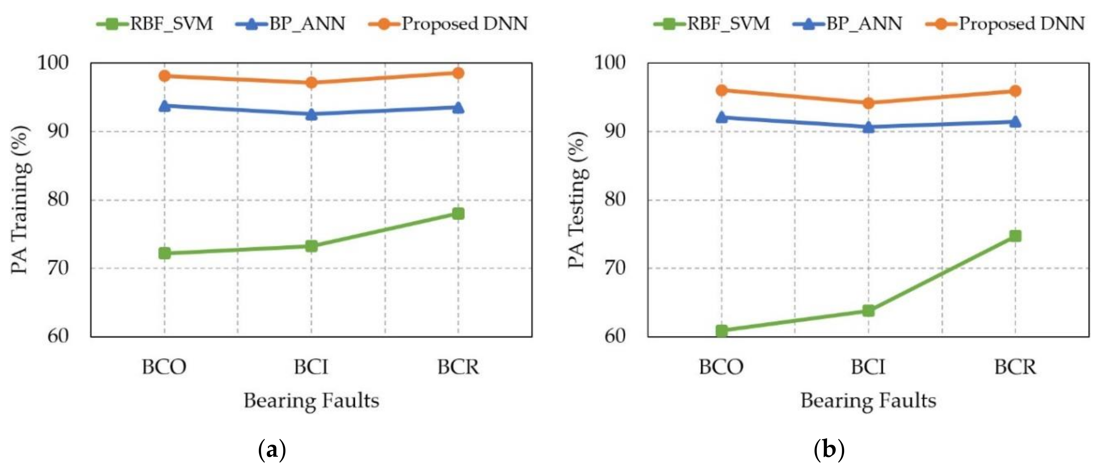
A comparison of the prediction performance of the proposed DNN method with state-of-the-art approaches is presented in Table 2, including the radial-basis-function-based support vector machine regression (RBF_SVM) [29] and the backpropagation-based artificial neural network (BP_ANN) [14]. The RBF_SVM employs the support vector regression (SVR) method using the RBF kernel, which is suitable for a prediction case of the degradation level of bearing conditions. This RBF_SVM trained the same datasets preprocessed by the envelope analysis technique. The obtained results are obvious that the RBF_SVM performed poorly at predicting bearing degradation compared to others methods, as illustrated in Figure 7. Similarly, the same datasets of bearing EPS signals were provided as inputs to the BP_ANN for the training process using the backpropagation algorithm. This BP_ANN had the same hierarchical architecture as the proposed DNN, in which its weights were initialized with random values and the biases of the neurons were set up to zero. Its performance was lower than the proposed method, as demonstrated in Figure 7. The aforementioned approaches were trained and tested with the same datasets to provide a fair and suitable comparison. As a result, the proposed DNN approach outperformed the existing methods in predicting the degradation level of each bearing defect collected simultaneously under different crack size conditions with a high average accuracy of 97.93% for training and 95.38% for testing.
5. Conclusions
Correct assessment of the degradation of bearing defects is urgent for reliable bearing condition monitoring and appropriate period maintenance decision in rotary machines. This paper proposed a DNN-based method to provide an effective solution for bearing fault prediction using a large number of data samples collected from bearing defects. It is necessary to precisely estimate the fault severities of bearings which make up a dataset for training the DNN. Thus, an effective GDM-based window method was used only to obtain the characteristic fault frequency components from the obtained EPS signals for the HI calculation, which served as an efficient quantitative metric for estimation of the severity of bearing defects. These obtained HI values were then used as appropriate templates for training the DNN. Moreover, the proposed DNN was trained using the Adam optimization-based backpropagation algorithm and Xavier initialization method for enhancing the learning speed and accuracy of the DNN. Experimental results indicated that the proposed DNN method yielded better performance and higher average accuracy compared to state-of-the-art approaches in predicting the degradation level of primary bearing defect conditions (BCO, BCI, and BCR) under different crack sizes.
Author Contributions
All the authors have contributed equally to the conception and idea of the paper, implementing and analyzing the processing methods, evaluating and discussing the experimental results, and writing and revising this manuscript.
Funding
This work was supported by the Korea Institute of Energy Technology Evaluation and Planning (KETEP) and the Ministry of Trade, Industry & Energy (MOTIE) of the Republic of Korea (Grant No. 20181510102160). It was also supported in part by the Ministry of SMEs and Startups (MSS), Korea, under the “Regional Specialized Industry Development Program (R&D, P006800689)” supervised by the Korea Institute for Advancement of Technology (KIAT), and in part by the Leading Human Resource Training Program of Regional Neo industry through the National Research Foundation of Korea (NRF) funded by the Ministry of Science, ICT and future Planning (NRF-2016H1D5A1910564).
Conflicts of Interest
The authors declare no conflict of interest.
References
- Jardine, A.K.S.; Lin, D.; Banjevic, D. A review on machinery diagnostics and prognostics implementing condition-based maintenance. Mech. Syst. Signal Process. 2006, 20, 1483–1510. [Google Scholar] [CrossRef]
- Nguyen, P.; Kang, M.; Kim, J.-M.; Ahn, B.-H.; Ha, J.-M.; Choi, B.-K. Robust condition monitoring of rolling element bearings using de-noising and envelope analysis with signal decomposition techniques. Expert Syst. Appl. 2015, 42, 9024–9032. [Google Scholar] [CrossRef]
- Climente-Alarcon, V.; Antonino-Daviu, J.A.; Riera-Guasp, M.; Vlcek, M. Induction Motor Diagnosis by Advanced Notch FIR Filters and the Wigner-Ville Distribution. IEEE Trans. Ind. Electron. 2014, 61, 4217–4227. [Google Scholar] [CrossRef]
- Leite, V.C.M.N.; Silva, J.G.B.D.; Torres, G.L.; Veloso, G.F.C.; Silva, L.E.B.D.; Bonaldi, E.L.; Oliveira, L.E.d.L.D. Bearing Fault Detection in Induction Machine Using Squared Envelope Analysis of Stator Current. In Bearing Technology; Darji, P.H., Ed.; InTech: Rijeka, Croatia, 2017; 67145p. [Google Scholar] [Green Version]
- Tian, J.; Morillo, C.; Azarian, M.H.; Pecht, M. Motor Bearing Fault Detection Using Spectral Kurtosis-Based Feature Extraction Coupled With K-Nearest Neighbor Distance Analysis. IEEE Trans. Ind. Electron. 2016, 63, 1793–1803. [Google Scholar] [CrossRef]
- Kang, M.; Kim, J.; Wills, L.M.; Kim, J.M. Time-Varying and Multiresolution Envelope Analysis and Discriminative Feature Analysis for Bearing Fault Diagnosis. IEEE Trans. Ind. Electron. 2015, 62, 7749–7761. [Google Scholar] [CrossRef]
- Du, Y.; Chen, Y.; Meng, G.; Ding, J.; Xiao, Y. Fault Severity Monitoring of Rolling Bearings Based on Texture Feature Extraction of Sparse Time–Frequency Images. Appl. Sci. 2018, 8, 1538. [Google Scholar] [CrossRef]
- Nguyen, H.; Kim, J.; Kim, J.-M. Optimal Sub-Band Analysis Based on the Envelope Power Spectrum for Effective Fault Detection in Bearing under Variable, Low Speeds. Sensors 2018, 18, 1389. [Google Scholar] [CrossRef] [PubMed]
- Zorzi, M. A New Family of High-Resolution Multivariate Spectral Estimators. IEEE Trans. Autom. Control 2014, 59, 892–904. [Google Scholar] [CrossRef]
- Zorzi, M. An interpretation of the dual problem of the THREE-like approaches. Automatica 2015, 62, 87–92. [Google Scholar] [CrossRef] [Green Version]
- Shen, C.; Wang, D.; Kong, F.; Tse, P.W. Fault diagnosis of rotating machinery based on the statistical parameters of wavelet packet paving and a generic support vector regressive classifier. Measurement 2013, 46, 1551–1564. [Google Scholar] [CrossRef]
- Kang, M.; Kim, J.; Kim, J.; Tan, A.C.C.; Kim, E.Y.; Choi, B. Reliable Fault Diagnosis for Low-Speed Bearings Using Individually Trained Support Vector Machines with Kernel Discriminative Feature Analysis. IEEE Trans. Power Electron. 2015, 30, 2786–2797. [Google Scholar] [CrossRef]
- Li, K.; Su, L.; Wu, J.; Wang, H.; Chen, P. A Rolling Bearing Fault Diagnosis Method Based on Variational Mode Decomposition and an Improved Kernel Extreme Learning Machine. Appl. Sci. 2017, 7, 1004. [Google Scholar] [CrossRef]
- Jia, F.; Lei, Y.; Lin, J.; Zhou, X.; Lu, N. Deep neural networks: A promising tool for fault characteristic mining and intelligent diagnosis of rotating machinery with massive data. Mech. Syst. Signal Process. 2016, 72–73, 303–315. [Google Scholar] [CrossRef]
- Chen, Z.; Deng, S.; Chen, X.; Li, C.; Sanchez, R.-V.; Qin, H. Deep neural networks-based rolling bearing fault diagnosis. Microelectron. Reliab. 2017, 75, 327–333. [Google Scholar] [CrossRef]
- Zhang, R.; Peng, Z.; Wu, L.; Yao, B.; Guan, Y. Fault Diagnosis from Raw Sensor Data Using Deep Neural Networks Considering Temporal Coherence. Sensors 2017, 17, 549. [Google Scholar] [CrossRef] [PubMed]
- L’Heureux, A.; Grolinger, K.; Elyamany, H.F.; Capretz, M.A.M. Machine Learning with Big Data: Challenges and Approaches. IEEE Access 2017, 5, 7776–7797. [Google Scholar] [CrossRef]
- Chi, M.; Plaza, A.; Benediktsson, J.A.; Sun, Z.; Shen, J.; Zhu, Y. Big Data for Remote Sensing: Challenges and Opportunities. Proc. IEEE 2016, 104, 2207–2219. [Google Scholar] [CrossRef]
- Yin, J.; Chen, B.; Lai, K.R.; Li, Y. Automatic Dangerous Driving Intensity Analysis for Advanced Driver Assistance Systems From Multimodal Driving Signals. IEEE Sens. J. 2018, 18, 4785–4794. [Google Scholar] [CrossRef]
- Yin, J.; Chen, B. An Advanced Driver Risk Measurement System for Usage-Based Insurance on Big Driving Data. IEEE Trans. Intell. Veh. 2018. [Google Scholar] [CrossRef]
- Xu, Y.; Sun, Y.; Wan, J.; Liu, X.; Song, Z. Industrial Big Data for Fault Diagnosis: Taxonomy, Review, and Applications. IEEE Access 2017, 5, 17368–17380. [Google Scholar] [CrossRef]
- Bediaga, I.; Mendizabal, X.; Arnaiz, A.; Munoa, J. Ball bearing damage detection using traditional signal processing algorithms. IEEE Instrum. Meas. Mag. 2013, 16, 20–25. [Google Scholar] [CrossRef]
- Wang, D.; Miao, Q.; Fan, X.; Huang, H.-Z. Rolling element bearing fault detection using an improved combination of Hilbert and wavelet transforms. J. Mech. Sci. Technol. 2009, 23, 3292–3301. [Google Scholar] [CrossRef]
- Hinton, G.E.; Osindero, S.; Teh, Y.-W. A fast learning algorithm for deep belief nets. Neural Comput. 2006, 18, 1527–1554. [Google Scholar] [CrossRef] [PubMed]
- Cai, J.; Gu, S.; Zhang, L. Learning a Deep Single Image Contrast Enhancer from Multi-Exposure Images. IEEE Trans. Image Process. 2018, 27, 2049–2062. [Google Scholar] [CrossRef] [PubMed]
- Kingma, D.; Ba, J. Adam: A Method for Stochastic Optimization. arXiv, 2014; arXiv:1412.6980. [Google Scholar]
- Krishna Kumar, S. On weight Initialization in Deep Neural Networks. arXiv, 2017; arXiv:1704.08863. [Google Scholar]
- De Myttenaere, A.; Golden, B.; Le Grand, B.; Rossi, F. Mean Absolute Percentage Error for regression models. Neurocomputing 2016, 192, 38–48. [Google Scholar] [CrossRef] [Green Version]
- Soualhi, A.; Medjaher, K.; Zerhouni, N. Bearing Health Monitoring Based on Hilbert-Huang Transform, Support Vector Machine, and Regression. IEEE Trans. Instrum. Meas. 2015, 64, 52–62. [Google Scholar] [CrossRef]
Figure 1.
Experimental setup for machinery fault simulation. (a) Acquisition system of acoustic emission (AE) data; (b) Bearing primary fault conditions. BCO: bearing crack on the outer surface; BCI: bearing crack on the inner surface; BCR: bearing crack on the roller.
Figure 1.
Experimental setup for machinery fault simulation. (a) Acquisition system of acoustic emission (AE) data; (b) Bearing primary fault conditions. BCO: bearing crack on the outer surface; BCI: bearing crack on the inner surface; BCR: bearing crack on the roller.

Figure 2.
An overall flow diagram of the bearing defect degradation monitoring system. DNN: deep neural network.
Figure 2.
An overall flow diagram of the bearing defect degradation monitoring system. DNN: deep neural network.

Figure 3.
An overall description of estimating the bearing fault severity by the health-related indicator (HI) calculation. EPS: envelope power spectrum; GDM: Gaussian distribution model.
Figure 3.
An overall description of estimating the bearing fault severity by the health-related indicator (HI) calculation. EPS: envelope power spectrum; GDM: Gaussian distribution model.

Figure 4.
The flowchart of the proposed deep neural network (DNN) approach for predicting bearing fault degradation.
Figure 4.
The flowchart of the proposed deep neural network (DNN) approach for predicting bearing fault degradation.

Figure 5.
Estimation of the bearing defect severity corresponding to a bearing crack on the outer surface (BCO), a bearing crack on the inner surface (BCI), and a bearing crack on the roller (BCR) using the Gaussian distribution model (GDM)-based HI calculation.
Figure 5.
Estimation of the bearing defect severity corresponding to a bearing crack on the outer surface (BCO), a bearing crack on the inner surface (BCI), and a bearing crack on the roller (BCR) using the Gaussian distribution model (GDM)-based HI calculation.

Figure 6.
The prediction results of the degradation levels for each bearing condition (BCO, BCI, and BCR) under varying crack sizes using the proposed DNN-based method: (a) training and (b) testing.
Figure 6.
The prediction results of the degradation levels for each bearing condition (BCO, BCI, and BCR) under varying crack sizes using the proposed DNN-based method: (a) training and (b) testing.

Figure 7.
Degradation prediction of bearing defects according to varying crack sizes using the proposed DNN approach and other methods: (a) training and (b) testing.
Figure 7.
Degradation prediction of bearing defects according to varying crack sizes using the proposed DNN approach and other methods: (a) training and (b) testing.


Table 1.
The values of the characteristic defect frequencies at different crack sizes. BPFO: ball pass frequency of the outer surface; BPFI: ball pass frequency of the outer surface; BSF: ball spin frequency.
Table 1.
The values of the characteristic defect frequencies at different crack sizes. BPFO: ball pass frequency of the outer surface; BPFI: ball pass frequency of the outer surface; BSF: ball spin frequency.
| Crack sizes | Length (mm) | Width (mm) | Depth (mm) |
| 3 | 0.35 | 0.30 | |
| 6 | 0.49 | 0.50 | |
| 12 | 0.60 | 0.50 | |
| Shaft speed | 500 revolutions per minute (r/min) | ||
| Defect frequencies | BPFO = 43.68 Hz, BPFI = 64.65 Hz, and 2 × BSF = 41.44 Hz | ||
Table 2.
Accuracy of the proposed DNN approach in predicting the degradation levels of bearing defects. RBF_SVM: radial-basis-function-based support vector machine regression; BP_ANN: backpropagation-based artificial neural network.
Table 2.
Accuracy of the proposed DNN approach in predicting the degradation levels of bearing defects. RBF_SVM: radial-basis-function-based support vector machine regression; BP_ANN: backpropagation-based artificial neural network.
| Methodologies | The Prediction Accuracy (PA) of Bearing Fault Degradation Levels | |||||
|---|---|---|---|---|---|---|
| Training (%) | Testing (%) | |||||
| BCO | BCI | BCR | BCO | BCI | BCR | |
| RBF_SVM [29] | 72.19 | 73.26 | 78.01 | 60.88 | 63.79 | 74.70 |
| BP_ANN [14] | 93.76 | 92.53 | 93.50 | 92.08 | 90.67 | 91.45 |
| Proposed DNN | 98.14 | 97.12 | 98.54 | 96.05 | 94.17 | 95.91 |
© 2018 by the authors. Licensee MDPI, Basel, Switzerland. This article is an open access article distributed under the terms and conditions of the Creative Commons Attribution (CC BY) license (http://creativecommons.org/licenses/by/4.0/).
Share and Cite
MDPI and ACS Style
Nguyen, H.N.; Kim, C.-H.; Kim, J.-M. Effective Prediction of Bearing Fault Degradation under Different Crack Sizes Using a Deep Neural Network. Appl. Sci. 2018, 8, 2332. https://doi.org/10.3390/app8112332
AMA Style
Nguyen HN, Kim C-H, Kim J-M. Effective Prediction of Bearing Fault Degradation under Different Crack Sizes Using a Deep Neural Network. Applied Sciences. 2018; 8(11):2332. https://doi.org/10.3390/app8112332
Chicago/Turabian StyleNguyen, Hung Ngoc, Cheol-Hong Kim, and Jong-Myon Kim. 2018. "Effective Prediction of Bearing Fault Degradation under Different Crack Sizes Using a Deep Neural Network" Applied Sciences 8, no. 11: 2332. https://doi.org/10.3390/app8112332
Note that from the first issue of 2016, this journal uses article numbers instead of page numbers. See further details here.