Parameter Identification for Structural Health Monitoring with Extended Kalman Filter Considering Integration and Noise Effect


Abstract
:1. Introduction
2. EKF-Based Parameters Identification
3. Numerical Simulations
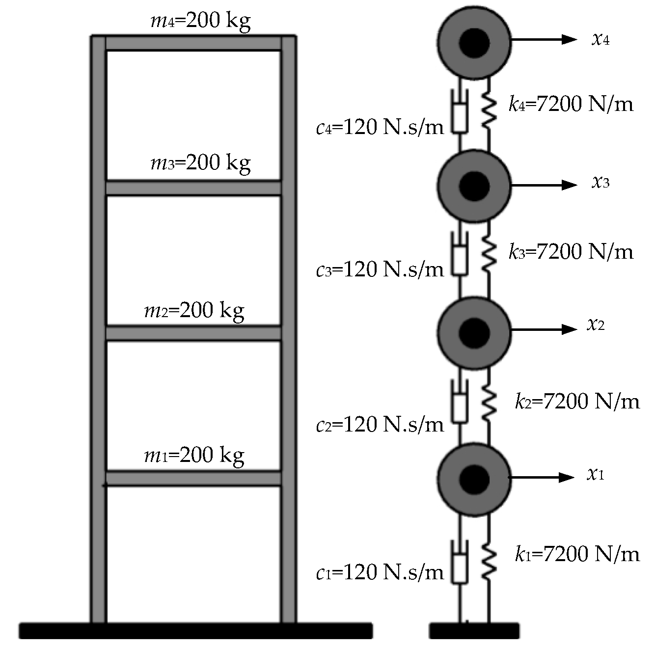
3.1. Numerical Model
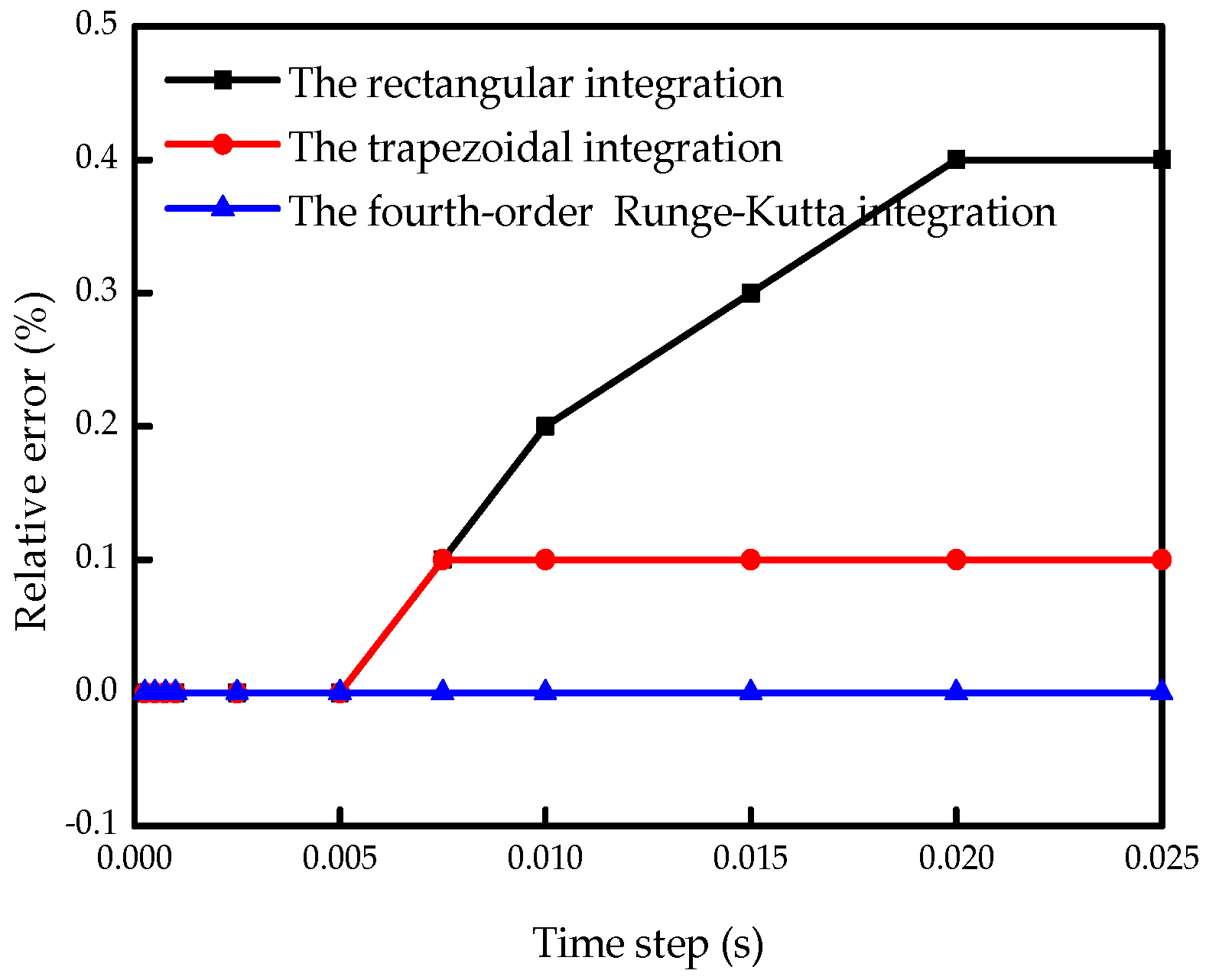
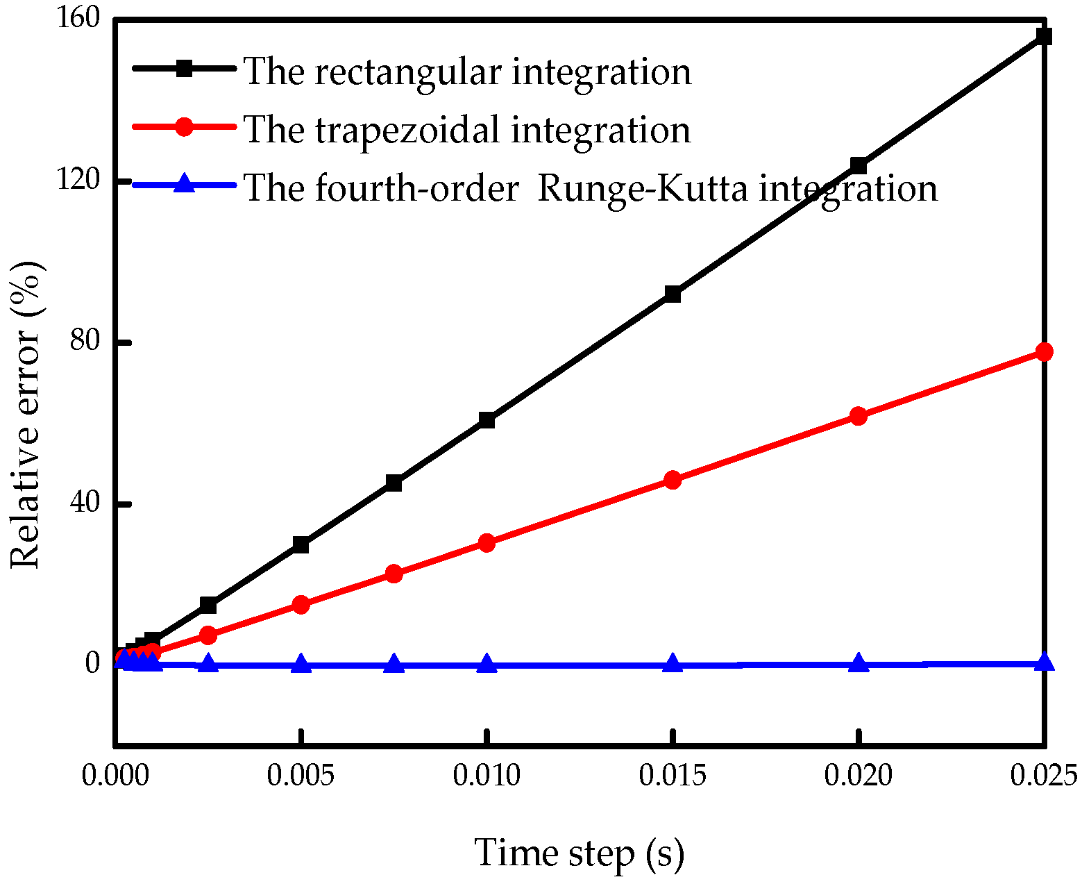
3.2. Parameter Identification with Different Integration Methods
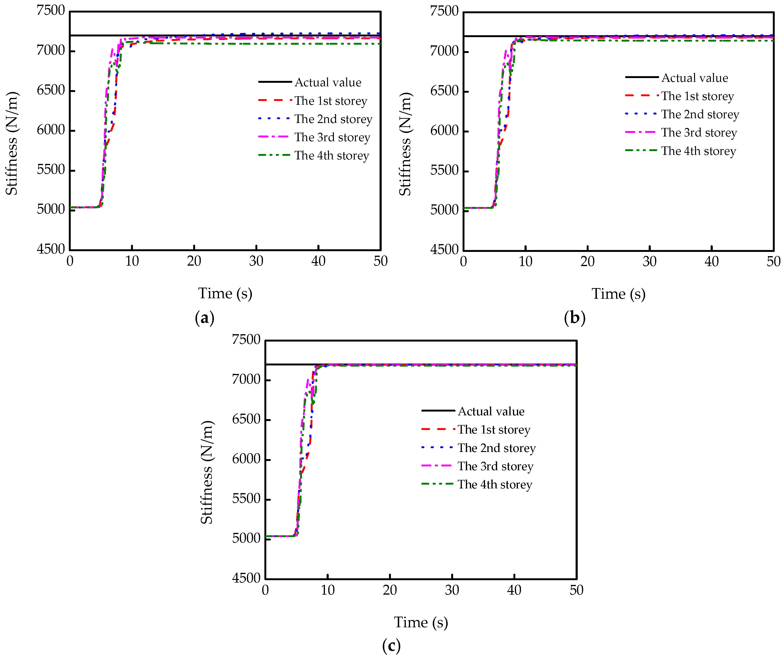
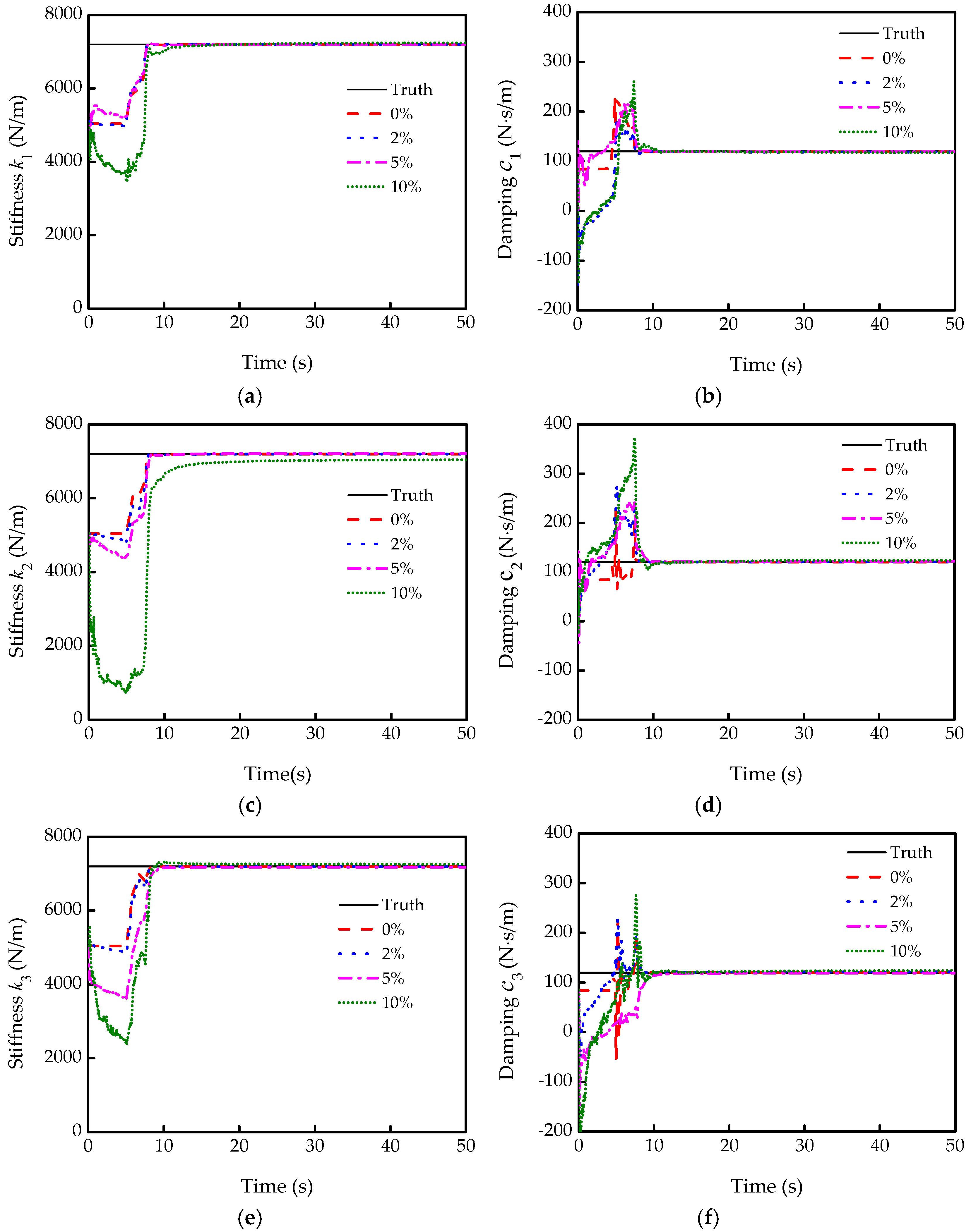
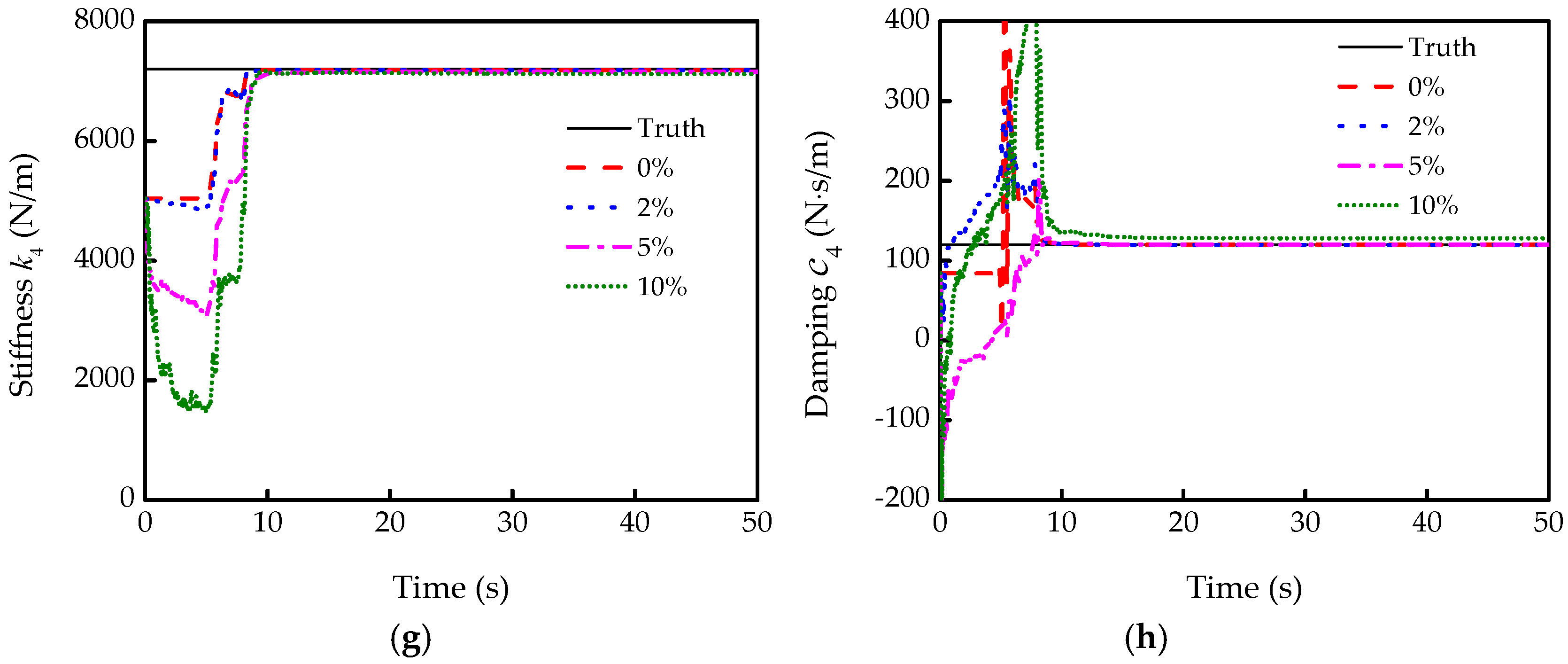
3.2.1. Stiffness Identification
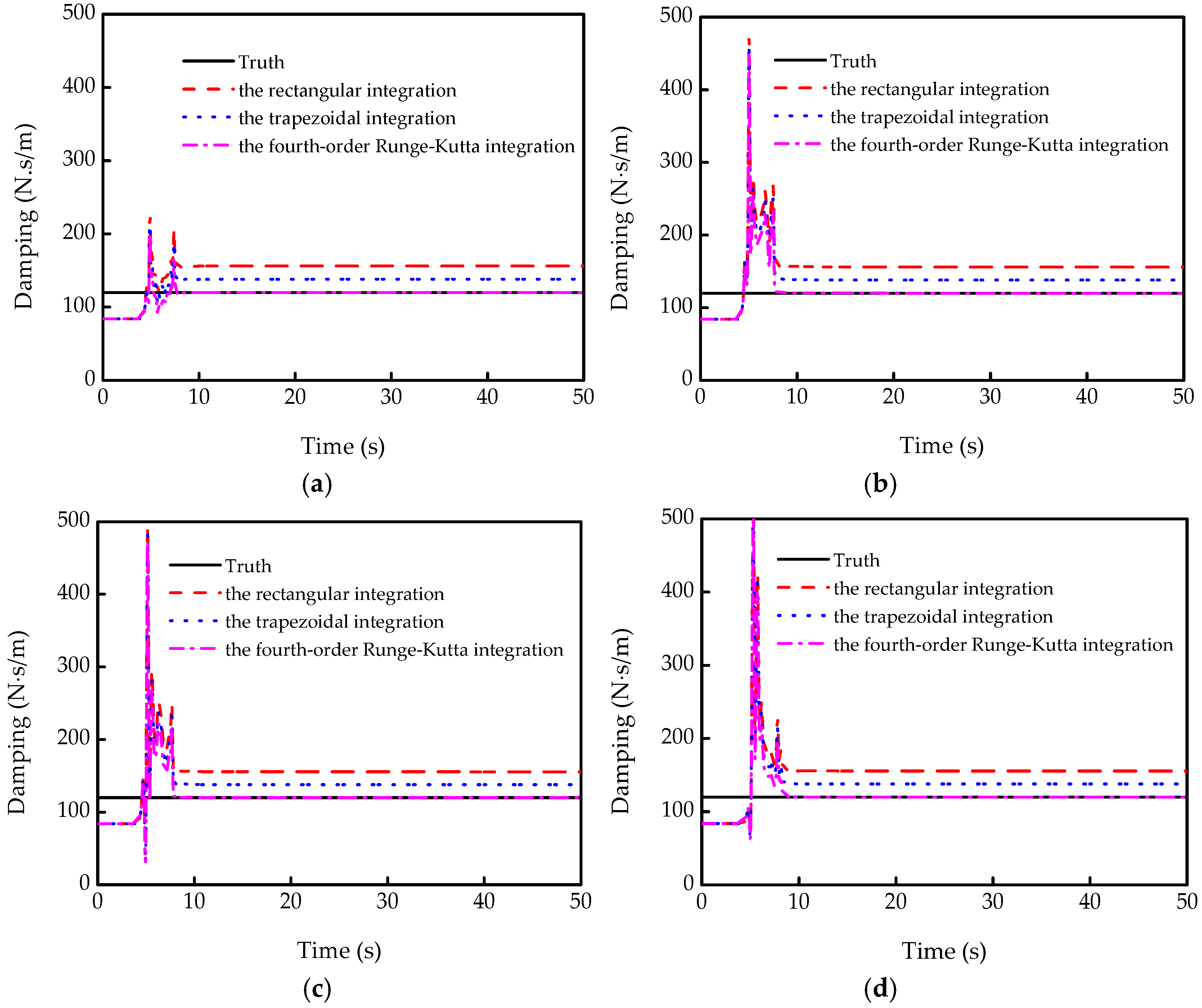
3.2.2. Damping Identification
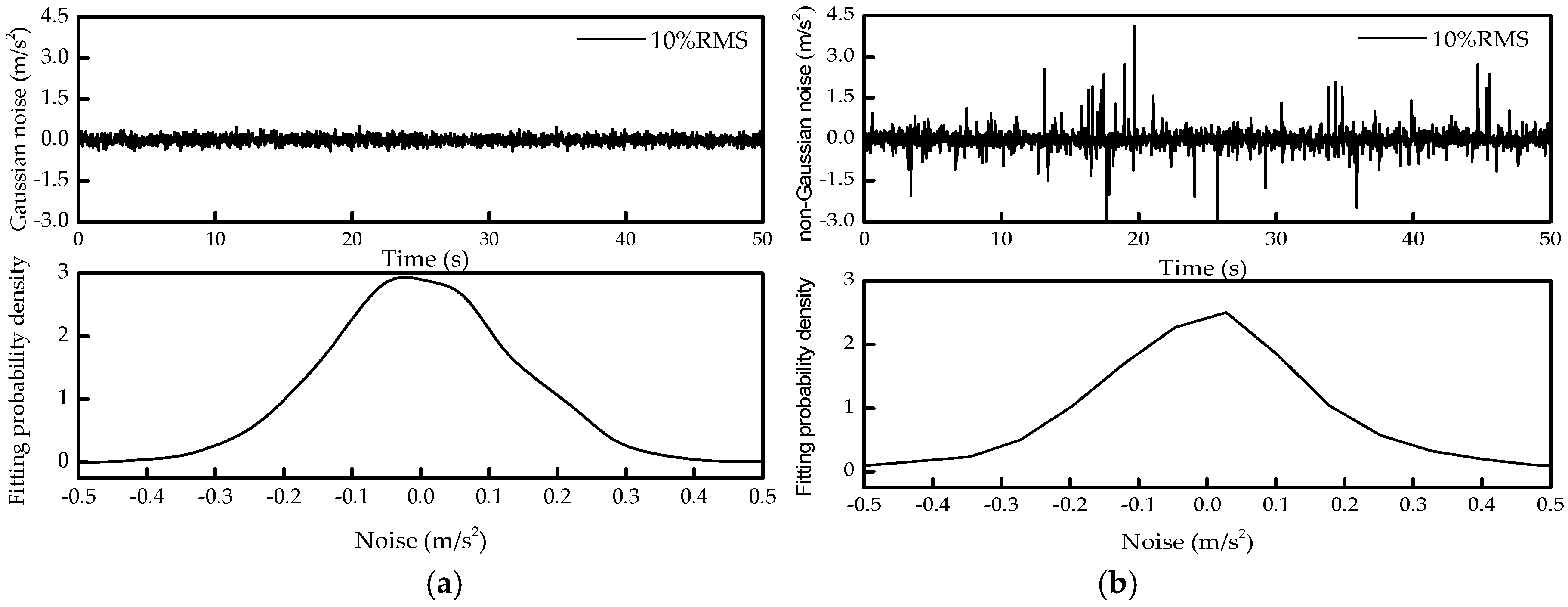
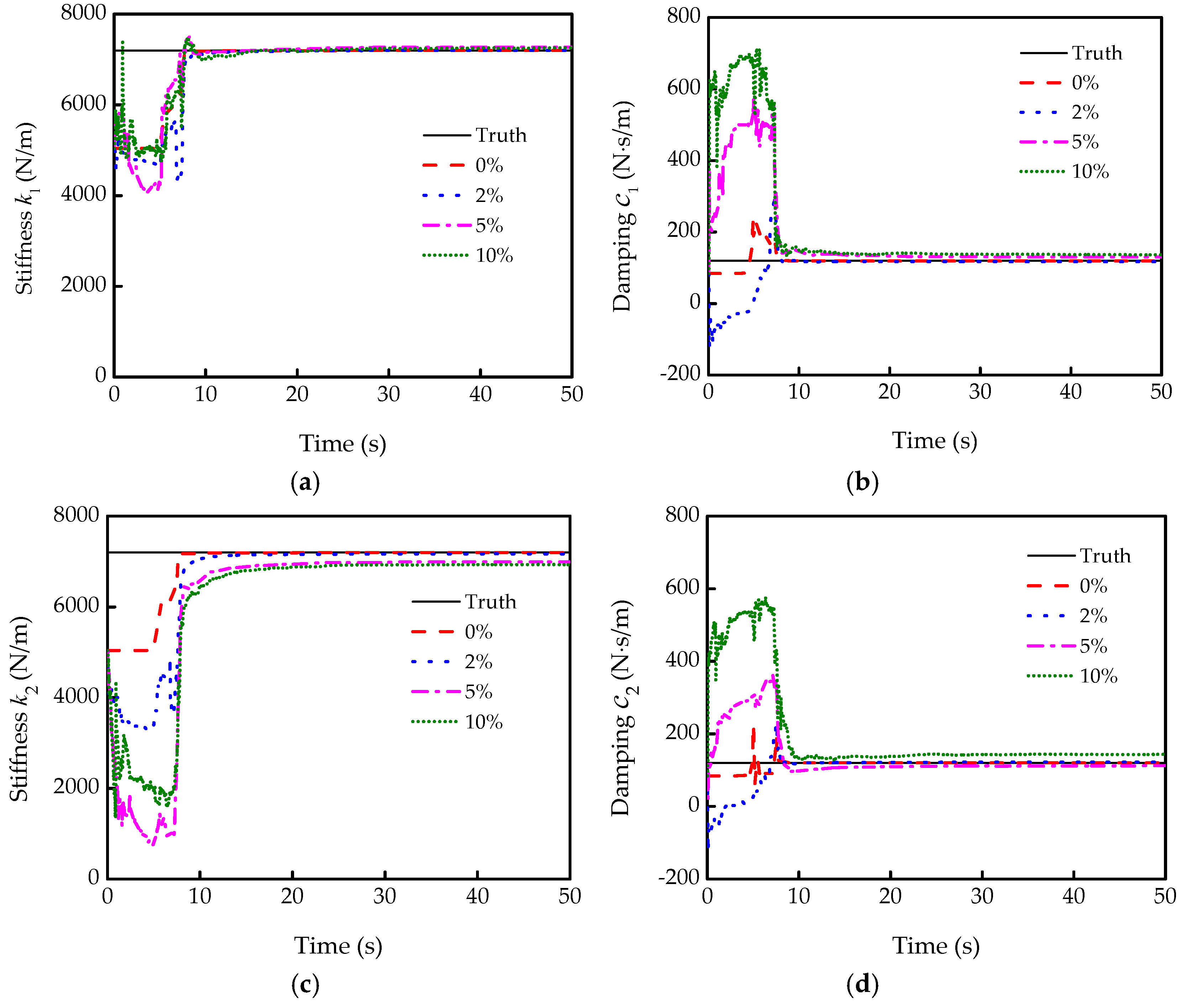
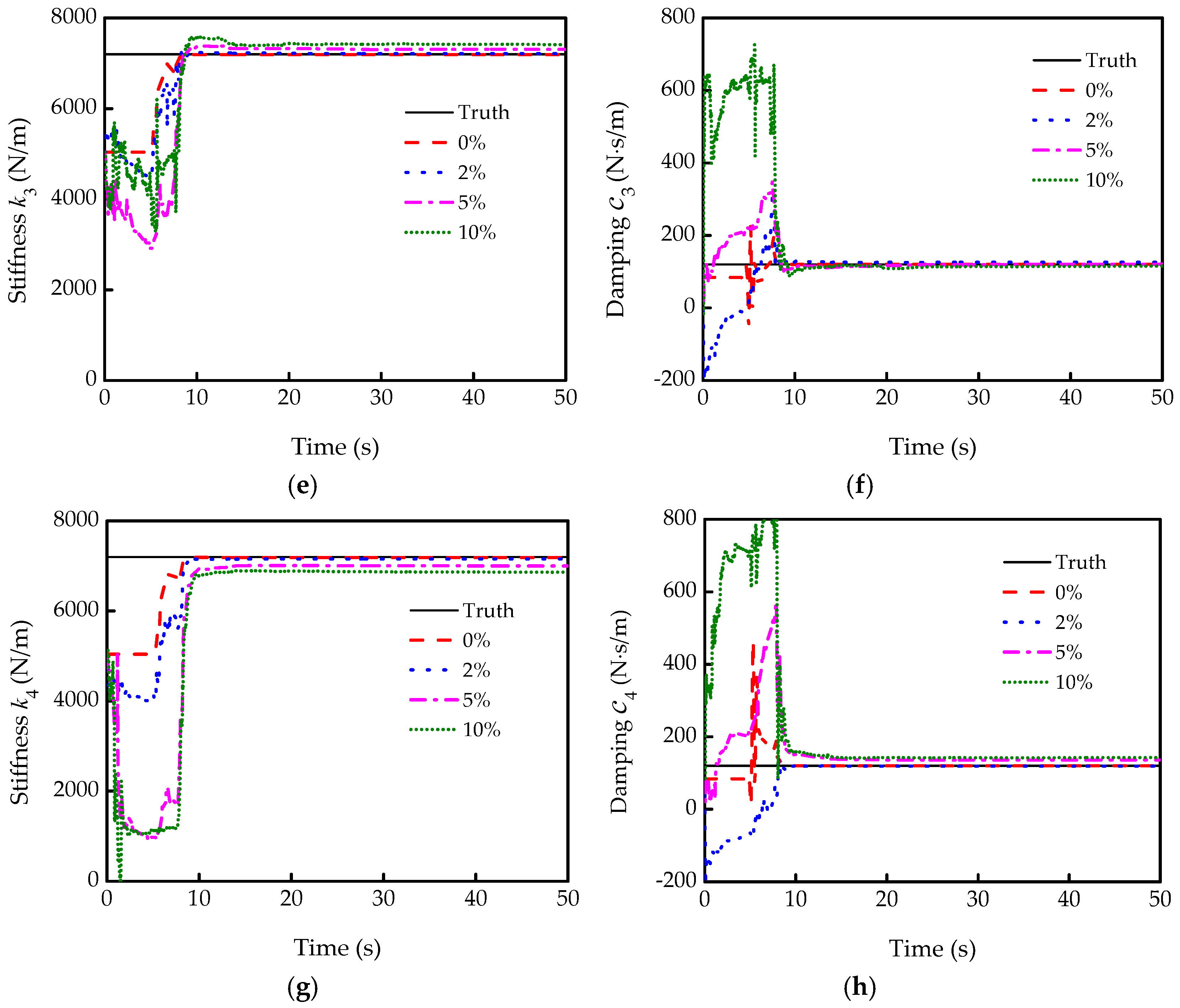
3.3. Parameter Identification under Gaussian and Non-Gaussian Noises
3.3.1. Parameter Identification under Gaussian Noises
3.3.2. Parameter Identification under Non-Gaussian Noises
4. Experiments
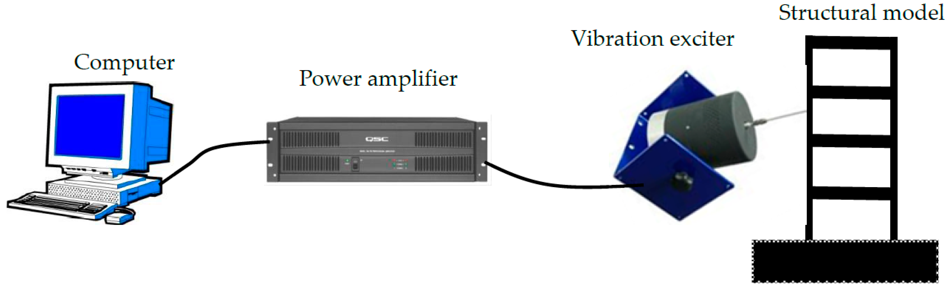
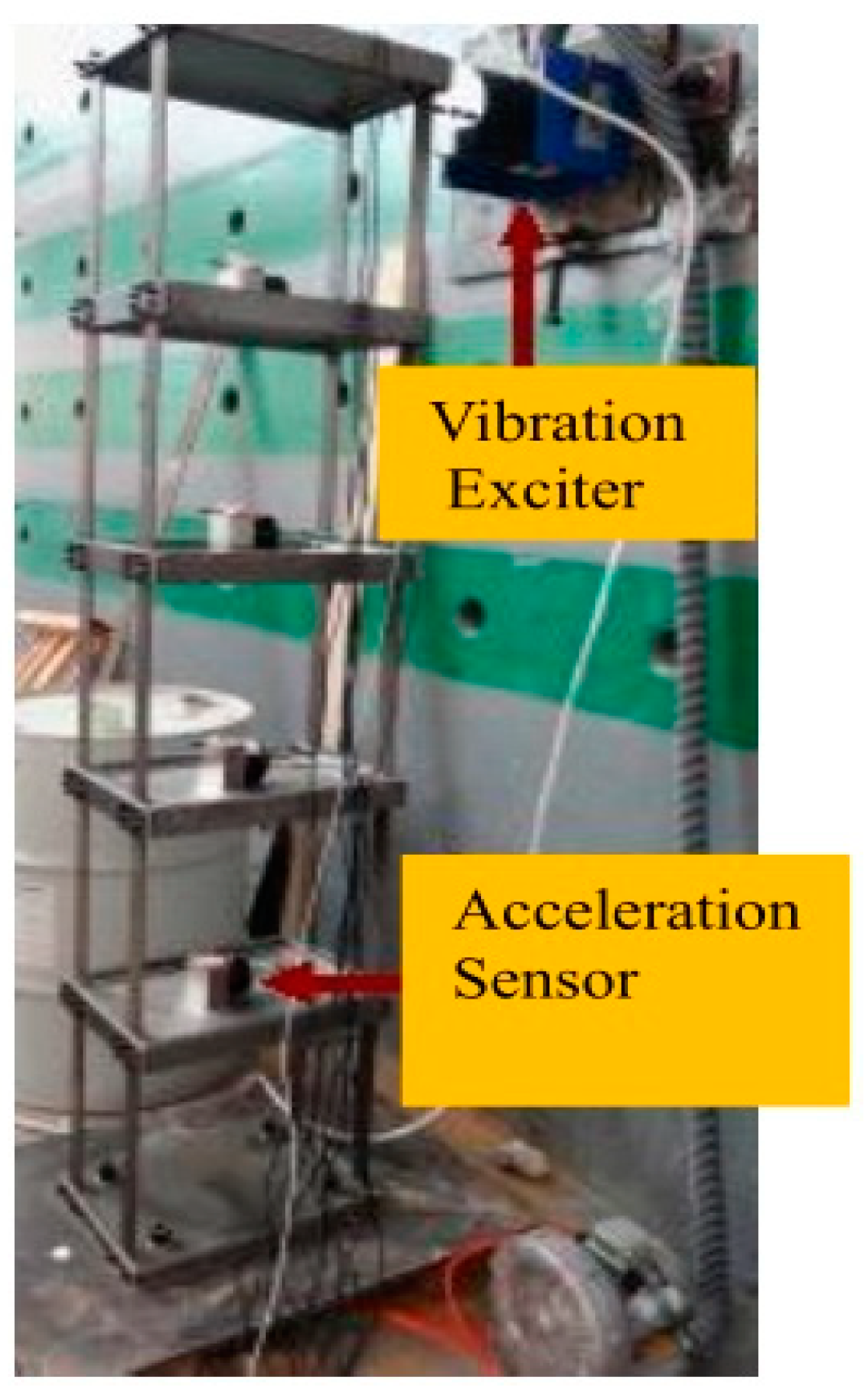
4.1. Excitation System
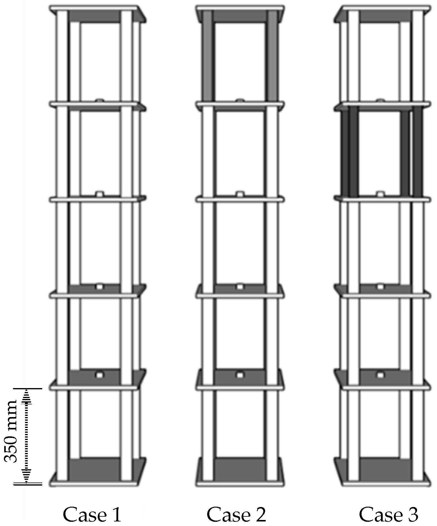
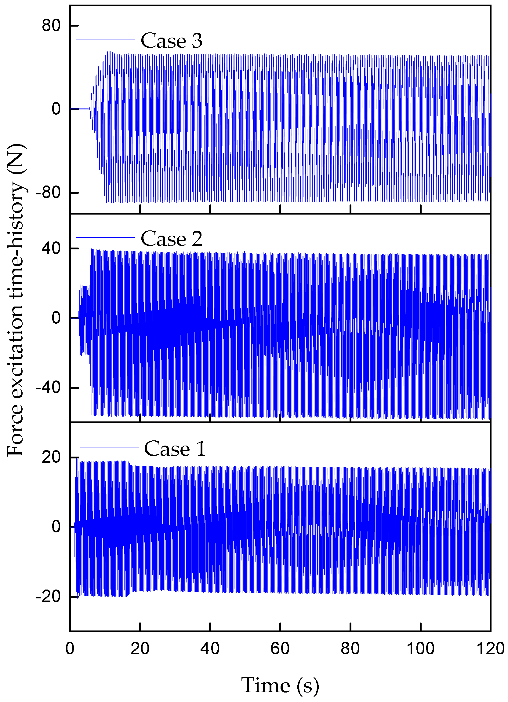
4.2. Experimental Model and Damage Cases
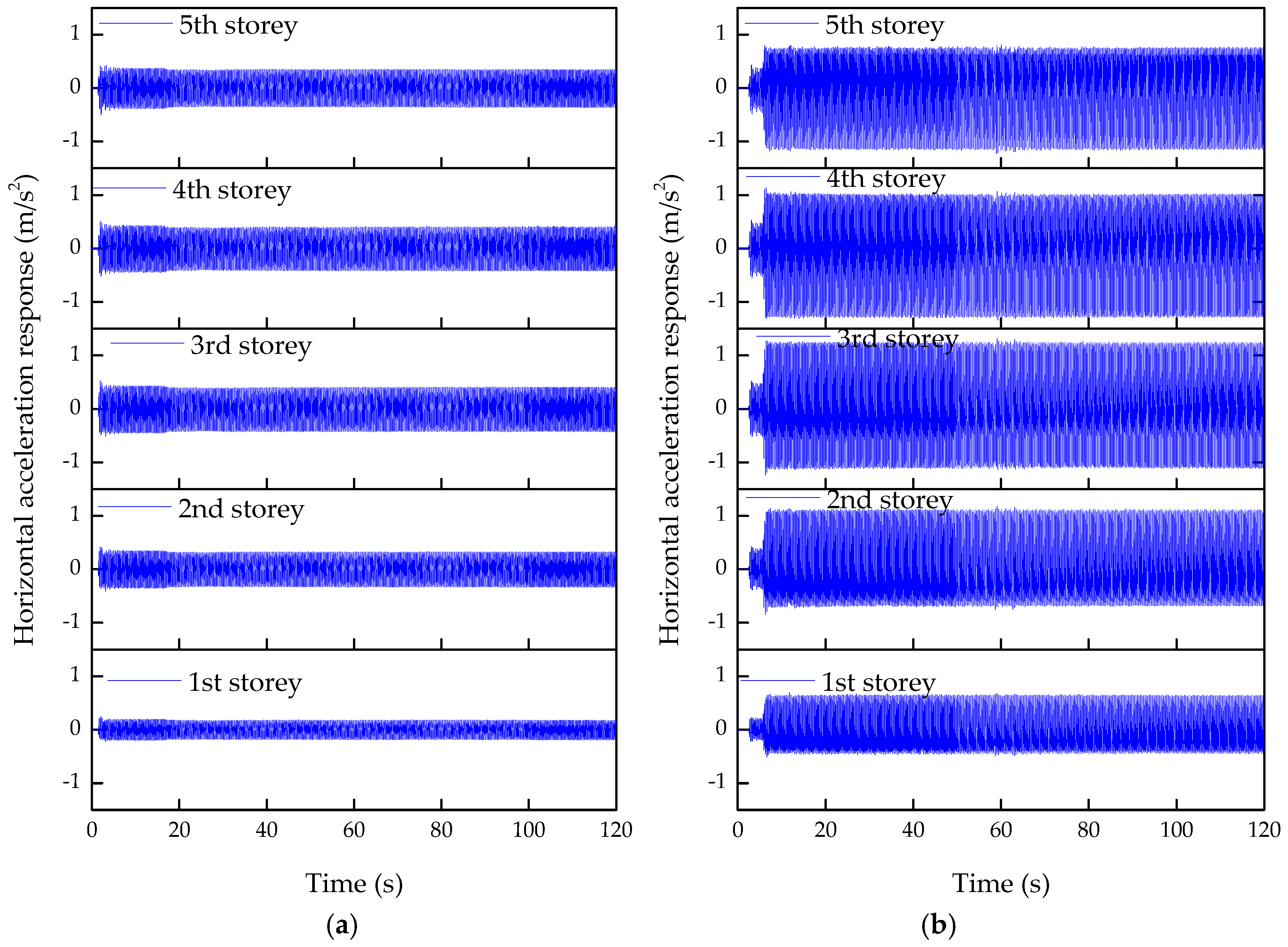
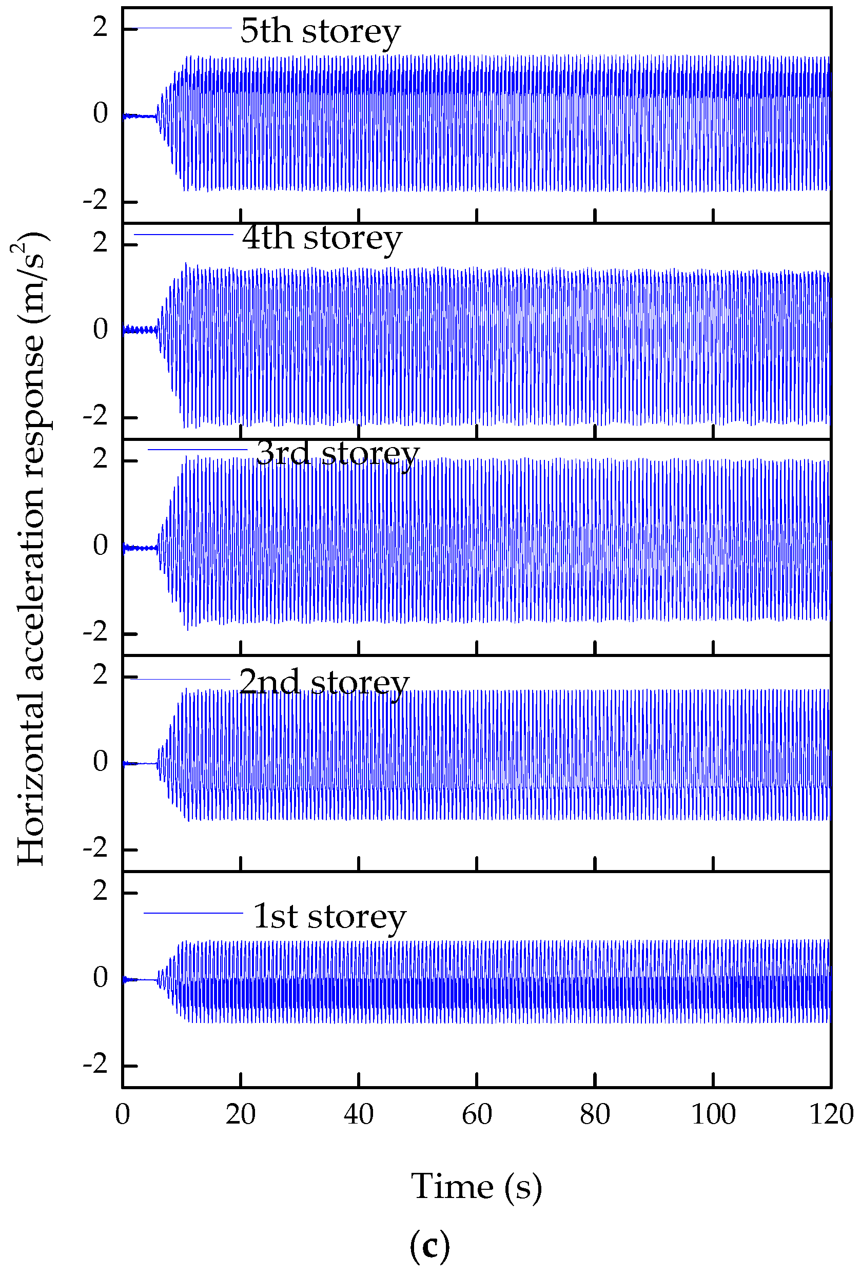
4.3. Experiment Implementation
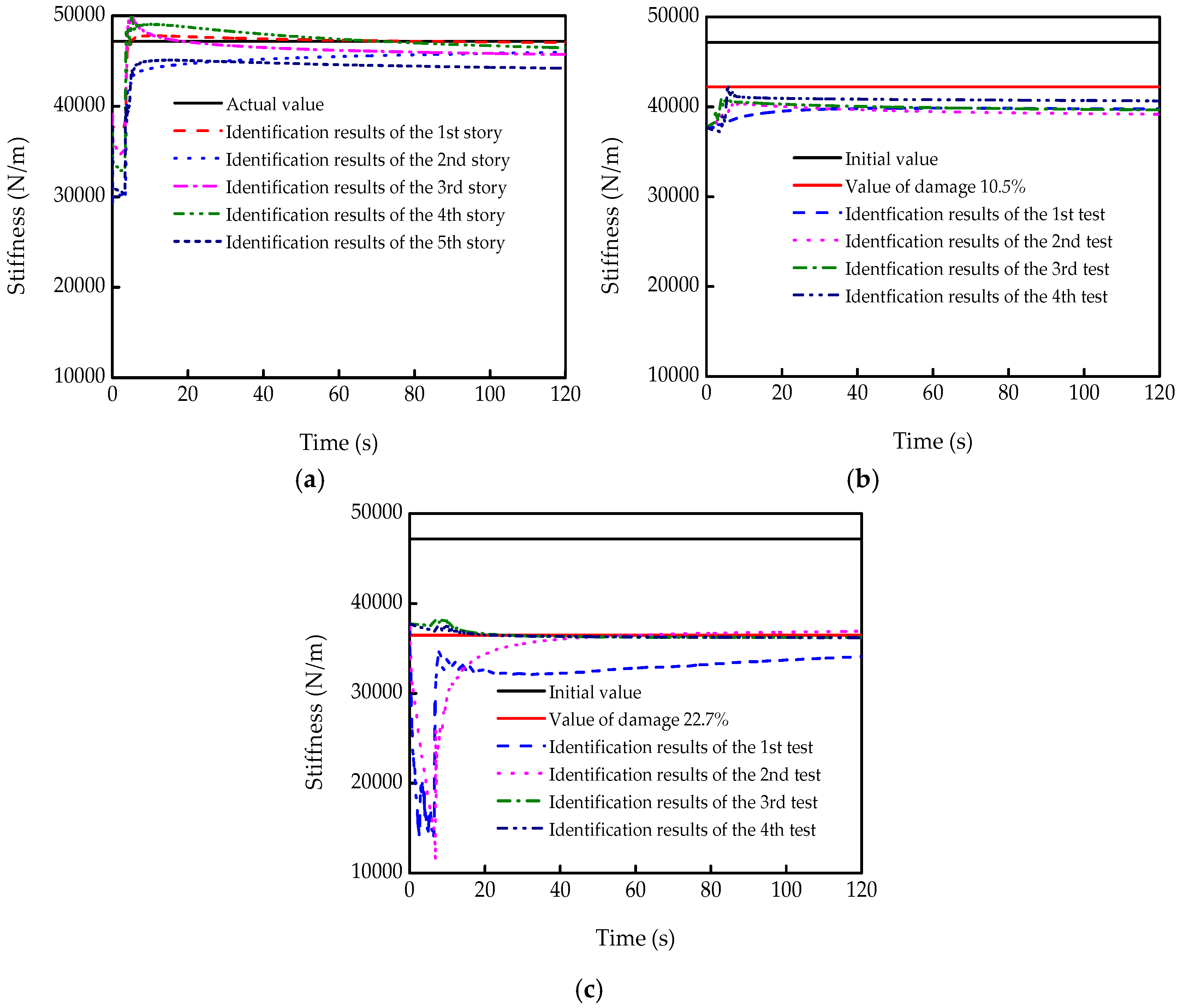
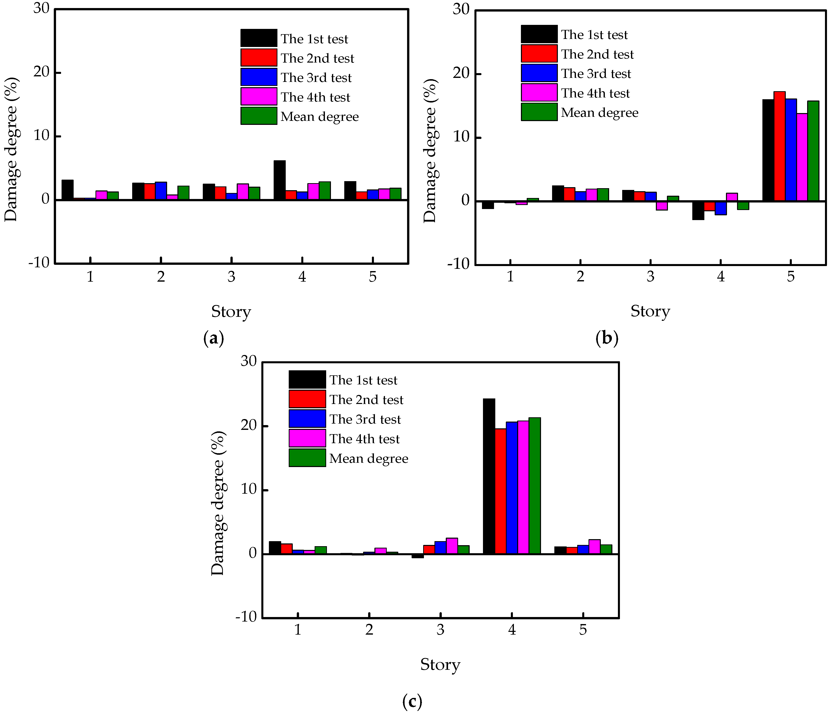
4.4. Structural Parameter Identification
5. Conclusions
Author Contributions
Funding
Conflicts of Interest
References
- Zhang, Z.G.; Guan, D. Experimental Investigation of Feedback Control of The rmoacoustic Oscillations using Least Mean Square-based Algorithms. J. Low Freq. Noise Vib. Act. Control 2015, 34, 153–168. [Google Scholar] [CrossRef]
- Yang, J.N.; Lin, S.L. Identification of Parametric Variations of Structures Based on Least Squares Estimation and Adaptive Tracking Technique. J. Eng. Mech. 2005, 131, 290–298. [Google Scholar] [CrossRef]
- Le, V.P.M.; Meenagh, D.; Minford, P.; Wickens, M. A Monte Carlo procedure for checking identification in DSGE models. J. Econ. Dyn. Control 2017, 76, 202–210. [Google Scholar] [CrossRef] [Green Version]
- Green, P.L.; Maskell, S. Estimating the parameters of dynamical systems from Big Data using Sequential Monte Carlo samplers. Mech. Syst. Signal Proc. 2017, 93, 379–396. [Google Scholar] [CrossRef]
- Nemeth, C.; Fearnhead, P.; Mihaylova, L. Sequential Monte Carlo Methods for State and Parameter Estimation in Abruptly Changing Environments. IEEE Trans. Signal Process. 2014, 2, 1245–1255. [Google Scholar] [CrossRef]
- Murakami, A.; Shinmura, H.; Ohno, S.; Fujisawa, K. Model identification and parameter estimation of elastoplastic constitutive model by data assimilation using the particle filter. Int. J. Numer. Anal. Methods Geomech. 2018, 42, 110–131. [Google Scholar] [CrossRef]
- Wang, H.Q.; Chen, J.; Brownjohn, J.M.W. Parameter identification of pedestrian’s spring-mass-damper model by ground reaction force records through a particle filter approach. J. Sound Vib. 2017, 411, 409–421. [Google Scholar] [CrossRef]
- Zhu, Z.L.; Meng, Z.Q.; Cao, T.T.; Zhang, Z.J.; Dai, Y.X. Particle filter-based robust state and parameter estimation for nonlinear process systems with variable parameters. Meas. Sci. Technol. 2017, 28, 065003. [Google Scholar] [CrossRef]
- Rakhshan, M.; Moula, E.; Shabani-nia, F.; Safarinejadian, B.; Khorshidi, S. Active noise control using wavelet function and network approach. J. Low Freq. Noise Vib. Act. Control 2016, 35, 4–16. [Google Scholar] [CrossRef] [Green Version]
- Wang, S.; Huang, S.L.; Wang, Q.; Zhang, Y.; Zhao, W. Mode identification of broadband Lamb wave signal with squeezed wavelet transform. Appl. Acoust. 2017, 125, 91–101. [Google Scholar] [CrossRef] [Green Version]
- Le, T.P. Use of the Morlet mother wavelet in the frequency-scale domain decomposition technique for the modal identification of ambient vibration responses. Mech. Syst. Signal Proc. 2017, 95, 488–505. [Google Scholar] [CrossRef]
- Das, B.; Pal, S.; Bag, S. A combined wavelet packet and Hilbert-Huang transform for defect detection and modelling of weld strength in friction stir welding process. J. Manuf. Process. 2016, 22, 260–268. [Google Scholar] [CrossRef]
- Nouri, K.; Loussifi, H.; Braiek, N.B. A comparative study on the identification of the dynamical model of multi-mass electrical drives using wavelet transforms. Int. J. Syst. Sci. 2014, 45, 2223–2241. [Google Scholar] [CrossRef]
- Chen, B.; Zhao, S.L.; Li, P.Y. Application of Hilbert-Huang Transform in Structural Health Monitoring: A State-of-the-Art Review. Math. Probl. Eng. 2014, 2014, 1–22. [Google Scholar] [CrossRef]
- Kalman, R.E. A new approach to linear filtering and prediction problems. J. Basic Eng. 1960, 82, 35–45. [Google Scholar] [CrossRef]
- Kalman, R.E.; Bucy, R.S. New Results in Linear Filtering and Prediction Theory. J. Basic Eng. 1961, 83, 95–108. [Google Scholar] [CrossRef] [Green Version]
- Jazwinsky, A.H. Stochastic Process and Filtering Theory; Mathematics in Science and Engineering: New York, NY, USA, 1970; p. 1730. [Google Scholar]
- Yun, C.B.; Shinozuka, M. Identification of nonlinear structural dynamic systems. J. Struct Mech. 1980, 8, 187–203. [Google Scholar] [CrossRef]
- Corigliano, A.; Mariani, S. Parameter identification in explicit structural dynamics: Performance of the extended Kalman filter. Comput. Meth. Appl. Mech. Eng. 2004, 193, 3807–3835. [Google Scholar] [CrossRef]
- Best, M.C.; Bogdanski, K. Extending the Kalman filter for structured identification of linear and nonlinear systems. Int. J. Model. Identif. Control 2017, 27, 114–124. [Google Scholar] [CrossRef] [Green Version]
- González, D.; Badías, A.; Alfaro, I.; Chinesta, F.; Cueto, E. Model order reduction for real-time data assimilation through Extended Kalman Filters. Comput. Meth. Appl. Mech. Eng. 2017, 326, 679–693. [Google Scholar] [CrossRef]
- Sen, S.; Bhattacharya, B. Online structural damage identification technique using constrained dual extended Kalman filter. Struct. Control Health Monit. 2017, 24, e1961. [Google Scholar] [CrossRef]
- Zhang, C.; Huang, J.Z.; Song, G.Q.; Chen, L. Structural damage identification by extended Kalman filter with l1-norm regularization scheme. Struct. Control Health Monit. 2017, 24, e1999. [Google Scholar] [CrossRef]
- Jin, C.H.; Jang, S.; Sun, X.R. An integrated real-time structural damage detection method based on extended Kalman filter and dynamic statistical process control. Adv. Struct. Eng. 2016, 20, 549–563. [Google Scholar] [CrossRef]
- Bedon, C.; Bergamo, E.; Izzi, M.; Noè, S. Prototyping and validation of MEMS accelerometers for structural health monitoring-The case study of the Pietratagliata cable-stayed bridge. J. Sens. Actuator Netw. 2018, 7, 30. [Google Scholar] [CrossRef]
- Bedon, C.; Morassi, A. Dynamic testing and parameter identification of a base-isolated bridge. Eng. Struct. 2014, 60, 85–99. [Google Scholar] [CrossRef]


| 2% Noise | 5% Noise | 10% Noise | ||||
|---|---|---|---|---|---|---|
| Gaussian | Non-Gaussian | Gaussian | Non-Gaussian | Gaussian | Non-Gaussian | |
| k1 | −0.008 | 0.024 | −0.018 | −0.360 | 0.554 | 0.744 |
| k2 | −0.010 | −0.418 | 0.163 | −2.881 | −2.236 | −3.701 |
| k3 | −0.118 | 0.161 | −0.381 | 1.504 | 0.822 | 3.013 |
| k4 | −0.231 | −0.656 | −0.632 | −2.782 | −1.112 | −4.697 |
| c1 | −1.223 | −2.519 | −0.676 | 8.475 | −2.091 | 13.992 |
| c2 | 0.515 | 1.678 | 1.547 | −6.665 | 3.140 | 19.436 |
| c3 | 1.147 | 5.020 | −0.911 | 0.398 | 3.356 | −4.037 |
| c4 | −0.292 | −0.749 | 0.078 | 13.508 | 6.556 | 18.886 |
| Specification | Size (mm) | Theoretical Story Stiffness (N/mm) | Measured Actual Story Stiffness (N/mm) |
|---|---|---|---|
| 1 | 350 × 40 × 4 | 49.20 | 47.17 |
| 2 | 350 × 36 × 4 | 44.28 | 42.22 |
| 3 | 350 × 32 × 4 | 39.36 | 36.48 |
| Damage Cases | Initial Stiffness | Damaged Stiffness | Damage Location | Damage Degree (%) |
|---|---|---|---|---|
| Case 1 | 47.17 | 47.17 | None | 0 |
| Case 2 | 47.17 | 42.22 | 5th story | 10.5 |
| Case 3 | 47.17 | 36.48 | 4th story | 22.7 |
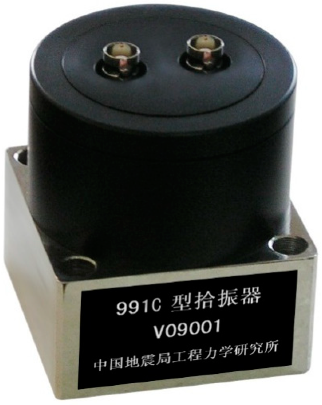
| Technical Indicators | Acceleration | Velocity |
|---|---|---|
| Sensitivity | 0.3 V·s2/m | 0.7 V·s/m |
| Maximum range | 20 m/s2 | 0.6 m/s |
| Passband | 0.1–100 Hz | 0.1–100 Hz |
| Resolution | 5 × 10⁻⁶ m/s2 | 2 × 10⁻⁶ m/s |
| Temperature range | −10 °C–+50 °C | −10 °C–+50 °C |
© 2018 by the authors. Licensee MDPI, Basel, Switzerland. This article is an open access article distributed under the terms and conditions of the Creative Commons Attribution (CC BY) license (http://creativecommons.org/licenses/by/4.0/).
Share and Cite
Xie, L.; Zhou, Z.; Zhao, L.; Wan, C.; Tang, H.; Xue, S. Parameter Identification for Structural Health Monitoring with Extended Kalman Filter Considering Integration and Noise Effect. Appl. Sci. 2018, 8, 2480. https://doi.org/10.3390/app8122480
Xie L, Zhou Z, Zhao L, Wan C, Tang H, Xue S. Parameter Identification for Structural Health Monitoring with Extended Kalman Filter Considering Integration and Noise Effect. Applied Sciences. 2018; 8(12):2480. https://doi.org/10.3390/app8122480
Chicago/Turabian StyleXie, Liyu, Zhenwei Zhou, Lei Zhao, Chunfeng Wan, Hesheng Tang, and Songtao Xue. 2018. "Parameter Identification for Structural Health Monitoring with Extended Kalman Filter Considering Integration and Noise Effect" Applied Sciences 8, no. 12: 2480. https://doi.org/10.3390/app8122480