An Experimental Investigation into Combustion Fitting in a Direct Injection Marine Diesel Engine

College of Power and Energy Engineering, Harbin Engineering University, Harbin 150001, China
*
Author to whom correspondence should be addressed.
Appl. Sci. 2018, 8(12), 2489; https://doi.org/10.3390/app8122489
Submission received: 16 November 2018
/
Revised: 29 November 2018
/
Accepted: 30 November 2018
/
Published: 4 December 2018
(This article belongs to the Special Issue Direct Injection Reciprocating Internal Combustion Engines)
Abstract
:The marine diesel engine combustion process is discontinuous and unsteady, resulting in complicated simulations and applications. When the diesel engine is used in the system integration simulation and investigation, a suitable combustion model has to be developed due to compatibility to the other components in the system. The Seiliger process model uses finite combustion stages to perform the main engine combustion characteristics and using the cycle time scale instead of the crank angle shortens the simulation time. Obtaining the defined Seiliger parameters used to calculate the engine performance such as peak pressure, temperature and work is significant and fitting process has to be carried out to get the parameters based on experimental investigation. During the combustion fitting, an appropriate mathematics approach is selected for root finding of non-linear multi-variable functions since there is a large amount of used experimental data. A direct injection marine engine test bed is applied for the experimental investigation based on the combustion fitting approach. The results of each cylinder and four-cylinder averaged pressure signals are fitted with the Seiliger process that is shown separately to obtain the Seiliger parameters, and are varied together with these parameters and with engine operating conditions to provide the basis for engine combustion modeling.
1. Introduction
Diesel engine combustion is an unsteady and discontinuous process, in which the fuel chemical energy is transferred to the work medium internal energy. Due to its complicated energy conversion process, modeling the diesel engine combustion is quite challenging to both engine designers and users [1]. When the engine is applied in an integrated system such as the diesel engine control system, after-treatment system, ship propulsion system, etc., the combustion details are not the main concern, but the main performance parameters of the engine, such as engine work, peak pressure, peak temperature, are strongly affected by the engine combustion process. A suitable approach on fitting diesel engine combustion process with a few parameters is useful for combustion modeling, where the mathematics analysis is essentially required to solve the rooting finding problems in particular for the experimental investigation, because plenty of experimental data needs to be handled and used in the multi-dimensional system of equations [2,3].
Diesel engine combustion process is varied in comparison with the other combustion machines, resulting in the specific theoretical investigation method. Recently there has been lots of diesel engine combustion research using both theoretical and experimental approaches. With the rapid development of three-dimension numerical calculation technology, the diesel engine combustion can be simulated in quite detailed ways to obtain the detailed combustion information [4,5]. A three-dimension simulation of diesel engine combustion requires the turbulence flow model, spray model and combustion model, among which the turbulence flow model plays an important role. Normally there are three ways to model the turbulence flow of the engine: Large Eddy Simulation (LES), Direct Numerical Simulation (DNS) and Reynolds-Averaged Navier-Stokes (RANS) [6]. Kahila et al. developed the LES together with a finite-rate chemistry model to investigate the engine dual-fuel ignition process [7]. Knudsen et al. proposed the compressible Eulerian numerical model to describe how liquid fuel injector nozzle geometry and operation strategies influence gas phase fuel distribution [8]. An et al. used the renormalization group K-epsilon model to describe the turbulent flow field and predict the soot particles evolution [9]. When modeling the turbulent flow, it is important to calculate the average chemical reaction rate and the turbulent combustion rate of fuel [10,11]. Yu et al. used the characteristic time combustion model coupled with the chemical kinetic mechanism to study the mixture formation’s influence on the smoke [12]. Cheng et al. studied the methyl esters of soybean and coconuts formed by spray combustion and related emissions of the diesel engine and further to the effect of EGR on these biodiesel fuel combustion [13]. The diesel engine spray models are mainly divided into homogeneous gaseous jet models and gas-liquid two phase models, and the latter use the gas and liquid two phases in modeling engine spray process [14,15,16].
Besides the three-dimension approaches in modeling the engine combustion process, the multi-zone models are also efficient tools. Compared with the commonly used single-zone models, the multi-zone models take into account the instantaneous details of combustion process, such as the formation and development of fuel spray, the relative motion of fuel droplets and air. A popularly used multi-zone combustion model is Hiroyasu’s fuel droplet evaporation combustion model [17], which includes the fuel injection sub-model, combustion thermodynamic calculation sub-model and emission generation sub-model. Zhang et al. used the in-cylinder steam injection method to establish a two-zone combustion model to research the waste heat recovery and NOx emission control [18]. Fang et al. built a two-dimension combustion model to study the effect of electric fields on the combustion characteristics of a lean-burning methane air mixture [19]. Xiang et al. proposed a two-zone combustion model in nature gas engine application and used this model for engine knocking predictions [20].
The diesel engine combustion measurement techniques include visualization, PIV (particle image velocimetry), LIF (laser induced fluorescence) and PDPA (phase Doppler particle anemometry). The PIV velocity measurement is a non-contact, transient and full-flow velocity measurement method, which has the advantages of not interfering with the quantitative information of the measured field and fast dynamic response [21,22]. LIF method produces relatively strong light signals with high spatial resolution and the fluorescence intensity is proportional to the incident light intensity so that it can be used to measure the concentration of substances [23]. The PDPA method depends on the frequency difference between the scattered light and the irradiated light of the moving particles, whose size is determined by analyzing the phase shift of the scattered light reflected or refracted by the spherical particles passing through the laser measuring body [24]. The diesel engine combustion experimental research supplemented with the theoretical investigation improve the engine combustion performance and reduces emissions.
Although the detailed engine combustion models are developed rapidly with the progress of simulation tool and experimental facilities, when the engine is used as a component of systems such as the control system, after treatment system and propulsion system, the engine combustion process has to meet the requirement of the system real-time characteristics. Mean value model is a time-domination model with cyclic time scale instead of the crank angle time scale, having the characteristics of fast calculation to get the engine main performance parameters, and it is commonly used in the control system and real-time dynamic simulation. Yin et al. introduced a turbocharged diesel engine model for hardware-in-the-loop simulation, which has the capability of observing engine state parameters and capturing engine transient response [25]. Sui et al. introduced a two finite stages Seiliger process model and simulates the engine combustion process by several parameters, which were applied in the ship propulsion system simulation [26]. Baldi et al. combined the zero-dimension and mean value models to calculate the engine performance parameters including the in-cylinder ones in relatively short simulation time [27]. Theotokatos et al. developed an extended engine mean value model to predict the thermodynamic parameters of two-stroke marine engine at different injection times [28]. Meanwhile, plenty of “black-box” methods such as multi-level hierarchical, neural networks, fuzzy logic, and wavelet networks are also applied in the modeling engine combustion process [29,30,31].
During the modeling engine combustion process, the experimental methods are frequently used together with theoretical analysis to parameterize the combustion process, in which the mathematics analysis is necessary to find the roots in the systems of equations deriving from the balance in the engine combustion process. Heat release rate calculation based on the measured in-cylinder pressure, energy conservation equation and empirical heat transfer formula is a fundamental method to obtain the engine combustion phenomena. On the other hand, when the heat release is known, the statistical analysis of a large amount of actual heat release can be used to build the heat release models based on the empirical formula or curve fitting [32]. The general semi-empirical formula for calculating heat release rate is Vibe formulas and the isosceles triangle combustion model [33,34]. In addition, if one only needs to know the engine in-cylinder main operating parameters under various conditions instead of the engine combustion details, the Seiliger process is the appropriate method for engine combustion modeling [26,35,36].
Nevertheless, it is critical to the mean value simulation model research that the derivation of Seiliger parameters such as the combustion parameters to give a global description of the combustion process obtains lots of experimental data or a deep theoretical investigation. Most of the researchers merely focused on obtaining the Seiliger parameters according to the engine experiments and ignoring the mathematics applications during the fitting process, resulting in the low accuracy. On the other hand, the Seiliger parameters of only one engine operating point, normally the nominal operating point, were used in these literatures, and the others were obtained based on the mathematical interpolation methods.
In the case of getting Seiliger parameters based on the combustion fitting process, the multiple variables non-linear system of equations has to be set up with equivalence criteria. When solving non-linear equations in engineering problems, the Bisection method, Secant method, Newton-Raphson method, etc. are usually used [37,38]. Sciniaka et al. introduced several iterative algorithms for solving equations and proposed an adaptive method based on the Newton-Raphson rooting method, which can better control the algorithm dynamics [39]. Furthermore, when more variables are chosen, the system of equivalence criteria becomes a multi-variable function and the Newton-Raphson method is a suitable way to find the roots of the system of equations. The Newton-Raphson method has a prominent advantage in that it has a square convergence around a single root of the equation f(x) = 0. It can also be used to find the multiple roots and the complex roots of the equation [40,41]. Meanwhile, the method converges linearly but can be super linear convergence by some conversions.
In this paper, an experimental investigation into combustion fitting is carried out based on the in-cylinder pressure signals measurement. With the processed measurement data, the Seiliger process model is introduced, and after determining the Seiliger parameters and equivalence criteria, the diesel engine measurement is fitted with Seilgier process model for engine combustion analysis. The fitting results of engine running at nominal point are shown in both single cylinder and four-cylinder average signals, in which the discrepancy of cylinder working condition can be obtained. Last but not least, the results of engine running at constant speed are discussed for further research on combustion fitting models on the systematic simulation of marine diesel engine applications.
2. Experiments
Diesel engine in-cylinder pressure measurement is the fundamental method to investigate the combustion process and an effective way to get insight into the combustion phenomena. In order to obtain the heat release, in-cylinder temperature, etc., a plenty of other engine measurements should be carried out, such as fuel consumption, inlet pressure, and engine speed.
2.1. Engine Test Bed Installation
The engine test bed is a MAN4L 20/27 diesel engine, which is a commonly used medium speed, direct injection marine diesel engine. The general data of the engine are listed in Table 1.
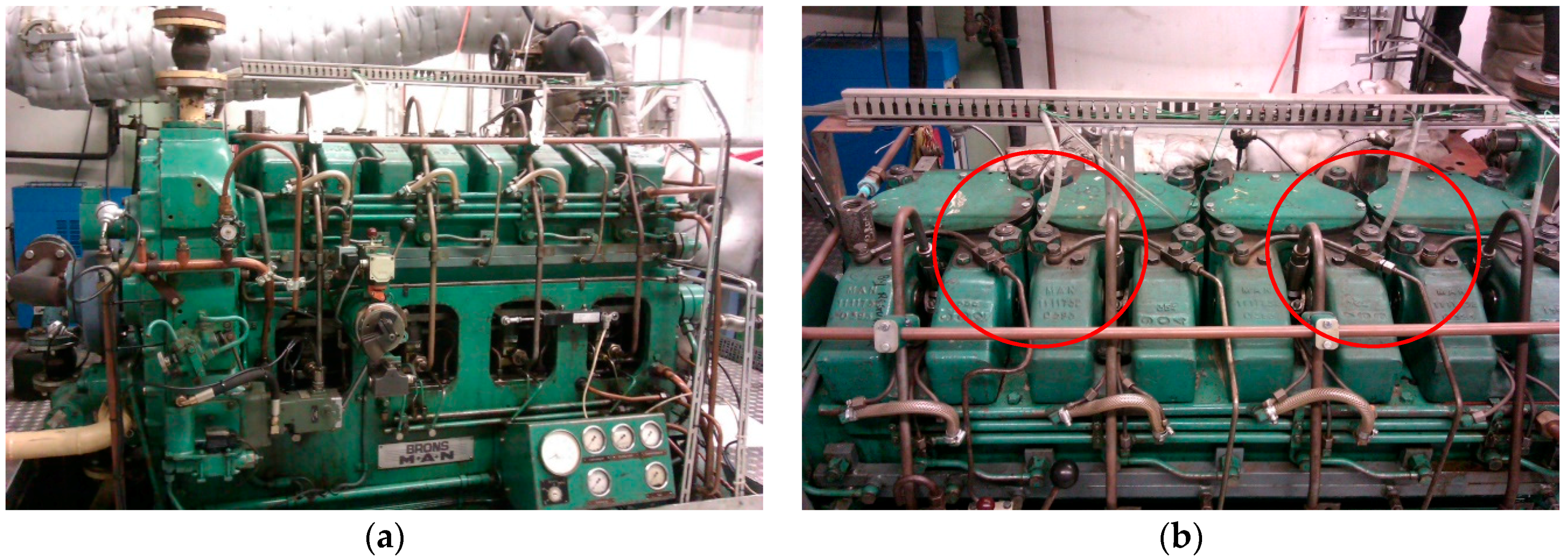
Figure 1 illustrates the engine test bed layout, which is installed in the laboratory with a hydraulic dynamometer for applying the engine load. The pressure sensors with a water cooling system are arranged in the cylinder head of each cylinder. Due to the two in-cylinder pressure sensors using one cooling tubule, in the two red circles, there are two pressure sensors mounted in each circle. There are also inlet receiver pressure and temperature, pressure and temperature before turbine, fuel consumption measurements, etc. Together with these measurements, the engine main performance parameters can be obtained to investigate the engine combustion process.
2.2. Measurements Procedures
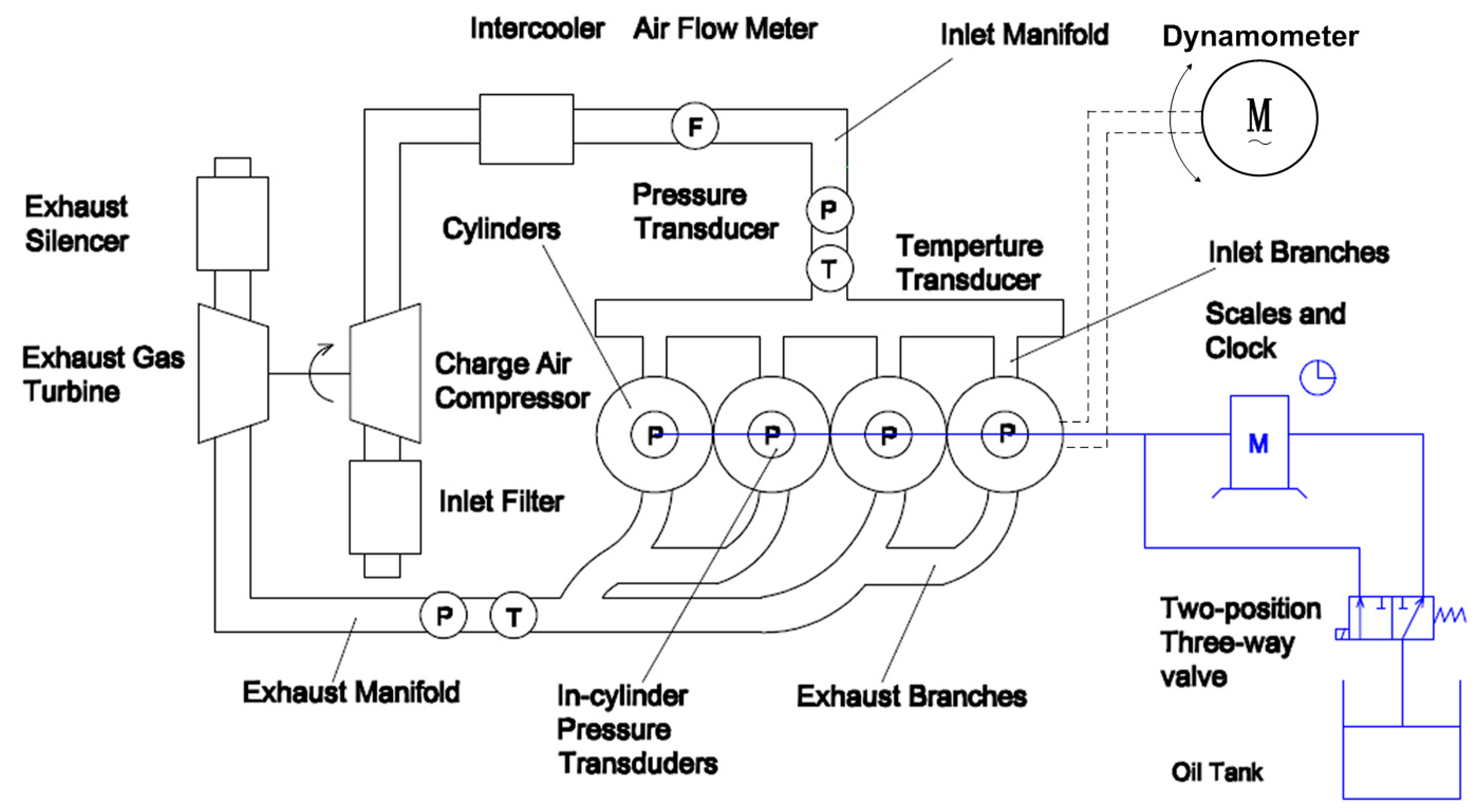
Figure 2 illustrates the engine test bed layout. The sensors arranged on the test bed are: in-cylinder pressure sensors, inlet pressure and temperature sensors, exhaust pressure and temperature sensors, air flow meters, hydraulic dynamometer, etc. The fuel flow measurement in the test bed uses the weighing scale and clock with a two-position three-way valve instead of a flow meter, which is a traditional method but ensures the accuracy of the fuel flow measurement.
2.3. Measurements samples Preparations
The marine diesel engine investigated in this paper is frequently used to drive a generator, therefore, two engine speed 900 rpm and 1000 rpm are selected in the measurement, and four operating points for each engine speed are measured (see Figure 3). In order to get the engine running points to be as thermodynamically stable as possible, the operating points at constant speeds were traversed alternatively up and down, as indicated by the arrows.
When the diesel engine is used for power generation, the engine speed has to be kept constant in order to ensure the constant frequency of current. Due to fixed current frequency f used in the marine power generation such as 50 Hz in China and 60 Hz in US, together with the number of poles P, the engine speed can be determined by Equation (1).
Therefore, the 50 Hz and 60 Hz are corresponding to 1000 r/min and 900 r/min when the poles numbers are selected to be 3 and 4 separately.
3. Methodology
3.1. In-Cylidner Measured Pressure Signals Processing
The measured in-cylinder pressure signals fluctuate especially in the peak pressure region, which will easily bring calculation errors during the combustion fitting process. Therefore, the measured pressure signals have to be processed firstly based on mathematics methods. On the other hand, some useful and effective methods can be used to improve the accuracy such as a pressure signals smooth approach based on the heat release calculation proposed by the author to ensure the accuracy of the signals’ application to some extent [32].
3.2. Seiliger Process and Seliger Process Parameters Obtain
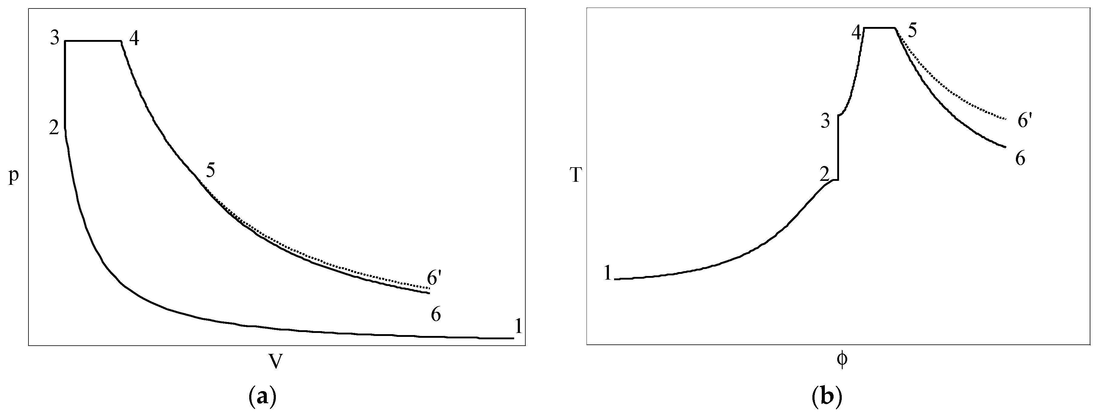
The Seiliger process is an efficient way to characterize the diesel engine combustion process, which divides the combustion process into finite stages to describe main phenomena of combustion characteristics. The definition and interpretation of Seiliger process and Seiliger parameters were described in author’s previous articles. Based on the stages number definition, there are 5-point Seiliger and 6-point Seiliger cycles [42]. Figure 4 shows the six-point Seiliger process model with both the basic and the advanced Seiliger process. The stages can be described as follows:
- 1–2:
- polytropic compression;
- 2–3:
- isochoric combustion;
- 3–4:
- isobaric combustion and expansion;
- 4–5:
- isothermal combustion and expansion;
- 5–6:
- polytropic expansion indicating a net heat loss, used when there is no combustion in this stage (basic);
- 5–6′:
- polytropic expansion indicating a net heat input caused by late combustion during expansion (advanced).
The Seiliger process can be described by a finite number of parameters that fully specify the process together with the initial (trapped) condition and the working medium properties. The definition of the Seiliger stages and the Seiliger parameters are given in Table 2. Among these Seiliger parameters a, b and c are the combustion parameters indicating the isochoric combustion stage, isobaric combustion stage and isothermal combustion stage respectively. The polytropic compression exponent ncomp and effective compression ratio rc model the polytropic compression process while the polytropic expansion exponent nexp and expansion ratio re model the polytropic expansion process. In the case that all the Seiliger parameters are known, the pressures, temperatures, work and heat in the various stages of the Seiliger cycle can be calculated.
Figure 5 shows how to obtain the Seiliger parameters based on measures in-cylinder pressure signals. The first line is the fit procedure to smooth the in-cylinder pressure signals, after which the Seiliger parameters are determined according to the combination of equivalence criteria between Seiliger process and in-cylinder process of the real engine. The Seiliger parameters are obtained from the ‘Seiliger fit model’ (model (4)), in which the fitting algorithms have to be investigated to improve the accuracy and speed the simulation time. Finally, the in-cylinder performance based on the Seiliger process characterizes the cylinder process and in particular the ‘combustion shape’ in order to compare the fitting results to the real engine (smoothed signals).
3.3. Combustion Fitting Approach
The Newton-Raphson method applied for a single variable function is briefly introduced. If the initial estimate of the root is xn, a tangent can be extended from the point [xn, f(xn)]. The point where this tangent crosses the x-axis represents an improved estimate of the root. The first derivative f′(xn) is equivalent to the slope of the tangent and can be derived on the basis of a geometrical interpretation (Figure 6) and an iteration scheme is constructed:
Then
While |xn+1 − xn+1| ≤ tolerance, the xn+1 can be considered to be the root of function f(x).
Furthermore, the Newton-Raphson method can be used to acquire the solution for a multi-variable function f(x). If the zero was considered to occur at x = x*, where x* is a vector, then the Taylor series for multi-variable function is applied. If xn is assumed to be the current estimation of the functions and xn+1 = xn + h, due to the demand that f(x*) = 0, the Taylor series is acquired:
If is assumed small enough to neglect, Equation (4) becomes:
When is replaced by matrix A:
Finally, the next estimate of xn+1 is obtained and used as the initial value of the next iteration and the iteration is terminated when the stop criteria are met.
3.4. Implementation in the Combustion Fitting Based on Seiliger Process
The Newton-Raphson multi-variable root finding method is applied to find the solution for the fitting of the (real) engine equivalence values by means of varying Seiliger process parameters. The Seiliger process is an engine combustion model to divide the engine working cycle into finite stages based on different Seiliger parameter numbers choosing. The case with four equivalence criteria as functions of four variables (Seiliger parameters) is taken as an example.
Seiliger parameters a, b, c and nexp are the variables in these equations and the differences between the calculated result from the equivalence criteria functions of the Seiliger process (pmax, Tmax, qin,Seiliger and wi,Seiliger) and the measured engine cycle(p3, T4, qin,measured and wi,measured) are the functions for which the zero has to be found. The other parameters in Equations (8)–(11) are considered to be constant but changed with engine working conditions. Therefore, the simulation model is important to determine them at different iteration steps rather than analytical method.
In summary, the Equations (8)–(11) are expressed by standard equation form
The five functions are set to a column vector as func:
A matrix PDE then is set to solve the derivatives:
Vect = −PDE/func
Vect is the increment or decrement of the root that is obtained from the previous step:
xi = xi + Vect (i) 1, 2, 3, 4
The partial derivatives of the elements in matrix PDE are obtained with numerical analysis rather than with an analytical method. The latter is impossible because some parameters in equivalence criteria functions are interdependent and a numerical method is used to avoid this problem.
Variable xi is changed one percent and then the partial derivatives are obtained relying on the local linearity.
4. Results and Analysis
4.1. The Process Pressure Signals of Four Cylinders
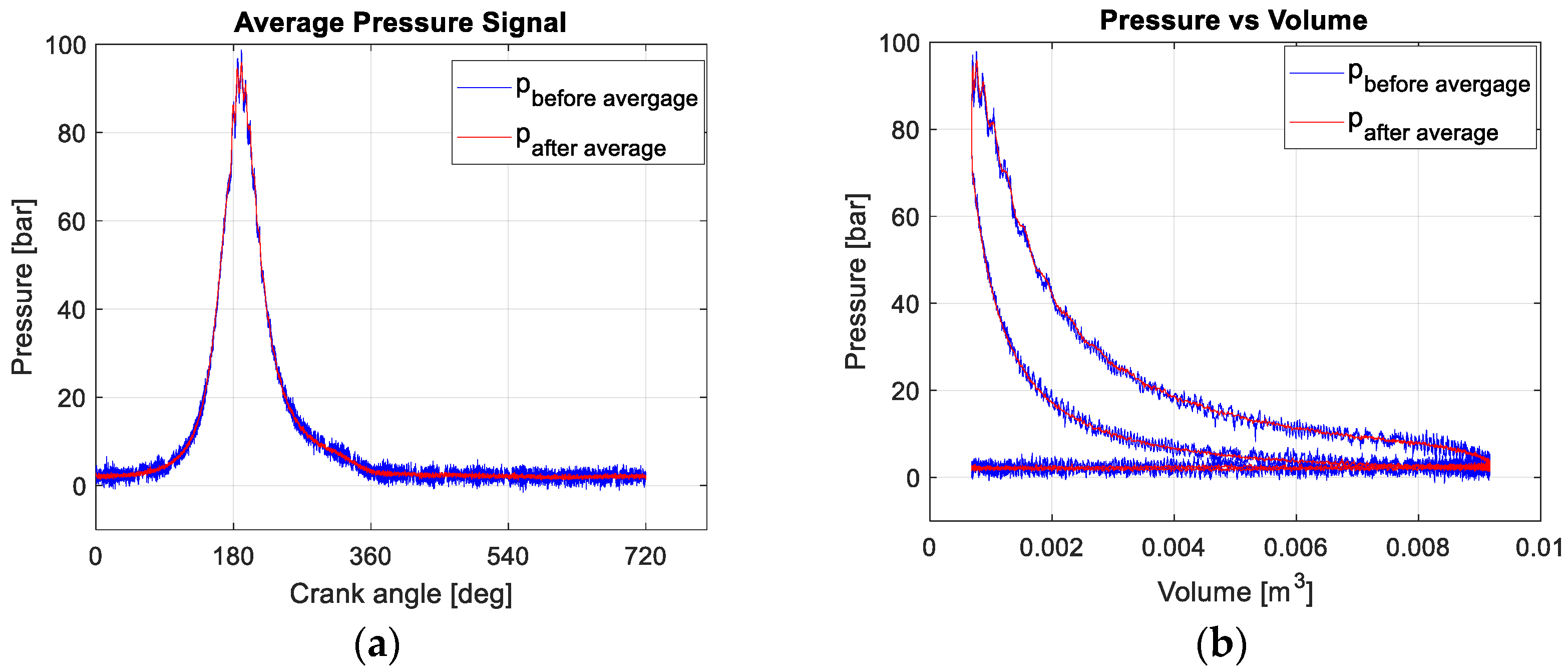
The frequency of logging the in-cylinder pressure signals is 0.02 ms meaning that there are around 6000 samples per cycle for this engine operating at 1000 rpm. Following the in-cylinder pressure measurements, the signals have to be processed first. In this engine test, 25 cycles were recorded for one operating point measurement selecting from the total measured cycle (around 200 cycles) and the in-cylinder pressure signals are averaged cycle by cycle to eliminate the fluctuation. Figure 7 shows the pressure signals before and after the cycle’s average in the p-φ and p-V diagram respectively, in which it is obvious to see that the in-cylinder pressure signals after 25 cycle’s average are smoother than before but the fluctuation still remains, especially in the peak pressure region.
Figure 8 shows the in-cylinder pressure signals of 4 cylinders. Due to the fire order in the multi-cylinder to keep the engine operating stable, this 4-cylinder diesel engine has 90 °CA differences between two cylinders and the fire order is 1-3-4-2 as shown in Figure 8a. In Figure 8b, the 4-cylinder pressure signals are moved together along with them being averaged on point by point in the overall cycle (the red curve). Figure 8c shows the zoom-in curves in the peak pressure region. Due to the pressure sensors mounted position, there are regular-looked waves in the peak pressure region. The tendency of the four cylinders is same in regards to the wave crest position and frequency, from which it seems that the four in-cylinder pressure signals average is necessary to eliminate the fluctuation effect in order to get the signals close to the reality.
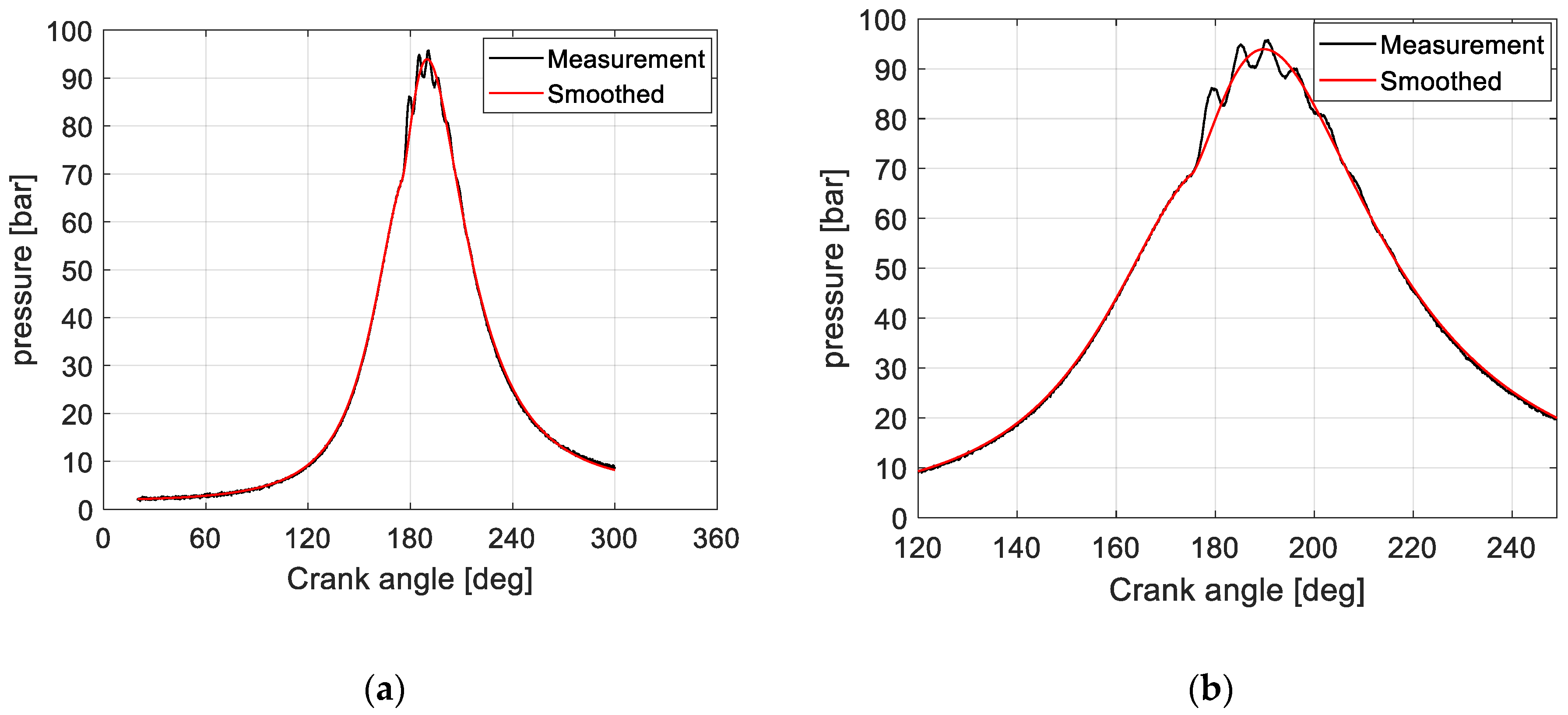
Although the in-cylinder pressure signals are smoothed according to cycle by cycle average and the four-cylinder average, the fluctuations still exist in particular in the peak pressure region. Since the waves are caused by the channel effect, the averaged method cannot solve these wave problems resulting in the difficulties for combustion fitting research. Therefore, the smoothing procedure has to continue to eliminate the channel effect’s influence as much as possible. Figure 9 compares the final smoothed pressure signals with measurement based on the new smooth method presented in reference [32]. According to Figure 9b, there is only one wave of the peak in-cylinder pressure region and for the other parts the pressure curve is smoothed sufficiently for the following combustion fitting investigation.
Regarding to the smoothing accuracy, as shown in Table 3, in the aspect of mathematics, there are ‘sum of squares due to error (SSE)’, ‘R-square’, ‘Adjusted R-square’, ‘Degrees of freedom in the error (DFE)’ and ‘Root mean squared error (RMSE)’ to evaluate the quality of fit. Also, the raw data and the smoothed results of the engine main performance parameters, such as Pmax, Tmax, PEO, TEO and Pi, are compared with each other to verify the signals processing accuracy.
4.2. The Combustion Fit Results of Engine Nominal Operating Point
With smoothed in-cylinder pressure signals and the definition of Seiliger process model, the engine combustion fitting can be carried out using the Newton-Raphson root finding method. The combustion fitting results of the nominal operating point are discussed firstly to validate and verify the approaches, after which the fitting results of engine running at generator conditions are presented for the further application of marine diesel engine combustion modelling.
4.2.1. Four-Cylinder Averaged Pressure Signals
According to definition of the basic and advanced Seiliger process presented in Section 3, the combustion fitting results of these two Seiliger process types are compared and analyzed in terms of the four-cylinder averaged pressure signals at engine nominal operating point. Table 4 shows the Seiliger parameters and engine performance parameters chosen in the system of equations as variables and equivalence criteria for basic and advanced Seiliger process models, which actually are the same as each other, although the engine performance parameter qin includes a different heat input definition as explained in Section 3.
Before combustion fitting numerical calculation, the Seiliger parameters ncomp, rc and ∆EO, which are not taken into account as the variables in the fitting process, have to be set as constants. Considering the engine operating conditions in reality, the ncomp is set to be 1.36 to indicate proper heat loss during engine compression process; the rc 13.107 means constant volumetric process occurring at top dead centre and ∆EO is 0 without regarding the effect of exhaust valve open. Then based on Equations (12)–(15), the system of equations of combustion fitting is set up. During the system of equations root finding procedure, the mathematic setting should be thought over, including initial values, iterations, termination criteria, etc.
The termination criteria for the iteration in this paper, which affect the accuracy and the calculation speed, in both basic and advanced Seiliger process models fitting is set as follows:
|p3 − pmax| ≤ 1 bar,
|T4 − Tmax| ≤ 1 K,
|qin,Seiliger − qin,measured| ≤ 10 J/kg,
|wi,Seiliger − wi,measured| ≤ 10 J/kg.
The combustion fitting results of both basic and advanced Seiliger process models are shown in Table 5, in which the Seiliger parameters values and heat input during the Seiliger parameters effect stages are compared. The values of a and b are the same of these two types, the latter’s small difference is caused by the numerical calculation errors. The value of c is quite different between these two Seiliger process models, together with heat input ratio in Seiliger stage 4–5 (isothermal process) large differences. In the basic Seiliger process, besides in stage 1–2 (isochoric process), the heat input occurs in isothermal process and the ratio is 36.02%, but in the advanced Seiliger process model it is only 16.53% with the others at 19.51% in stage 5–6 (expansion process), which means there is a very late combustion during operation of the engine.
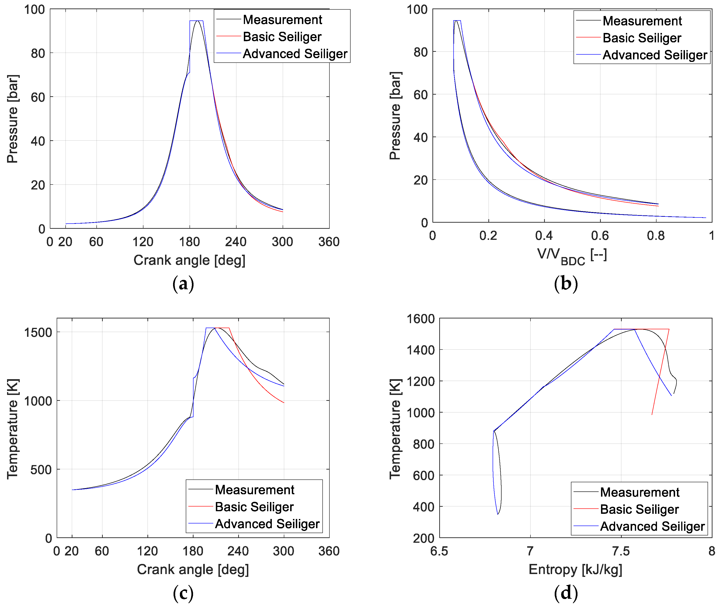
Figure 10 illustrates the basic and advanced Seiliger process models of combustion fitting results compared with the measurements in diversified diagrams. Figure 10a,b presents the comparison between pressure signals, due to relatively small scale, the difference among the three curves are not distinct. However, in the in-cylinder temperature diagram shown in Figure 10c, it is more likely to observe the trend and comparison of these curves, in which the basic and advanced Seiliger process before peak temperature completely coincide with each other and the duration of the isothermal process are different, and have a longer crank angle time with a larger c value in the basic Seiliger process model. The temperature at Exhaust Open (EO) in the basic Seiliger process is lower than that in the advanced Seiliger process model (around 150 K), which is caused by the late combustion occurring during expansion process in advanced Seiliger process model.
Figure 10d shows the fitting results compared with measurement in temperature-entropy diagram, which is even more clear to reveal the differences between the two Seiliger process models. The same trend as the in-cylinder temperature in Figure 10c before peak temperature and the two fitting curves are slightly different from the measurement. Nevertheless, the discrepancy among them in the expansion process is especially evident. The vertical curve in the T-S diagram means adiabatic expansion and the negative slope indicated heat input to the work medium and vice versa. As a result, the advanced Seiliger process model fitted the same case as the measurement with heat input in the expansion process and in the basic Seiliger process model, the result is totally different, i.e., heat loss during expansion.
Based on the fitting definition, when the basic Seiliger process model is used, the basic Seiliger process fitting shares the same equivalence criteria as the advanced Seiliger process model, but some of the heat enters the in-cylinder work medium in the isothermal process instead of the expansion process of advanced Seiliger process. From the fitting diagram, the advanced Seiliger process model fitting seems closer to the measurements, and when the ancient engine is operating with very late combustion, which is not expected, the advanced Seiliger process model is closer to the reality to describe the detailed phenomena of engine combustion. If the Seiliger process model fitting is used in the modern engine without late combustion, the basic process model fitting is preferred to avoid making errors in the heat input analysis with relatively simple modelling.
4.2.2. Each Cylinder Pressure Signals
The combustion fitting results discussed in the previous sections are based on the four-cylinder average pressure signals measurement in order to eliminate the measurement fluctuation effect. In fact, for the 4-cylinder diesel engine, four cylinders behave different performance to some extent in particular for the pressure signals but not too much due to engine operating balance demand. Table 6 shows the fitting results of the four cylinders respectively. The Seiliger parameters a and b are slightly different for the four cylinders, referring to the heat input ratio, there is maximum 2.22% difference for Seiliger parameter a (cylinder 1 and cylinder 2) and maximum 1.24% difference for Seiliger parameter b (cylinder 1 and cylinder 4).
As to Seiliger parameter c and nexp, there is much discrepancy such as 3.97% of Seiliger parameter c and 5.2% of Seiliger parameter nexp. This does not apply to cylinder 3, which has irregular cylinder fitting results. However, the fitting results of averaged in-cylinder pressure signals is not much affected by that of cylinder 3 and closed to the result of cylinders 1, 2 and 4. Although there are irregular cylinder fitting results, which are probably caused by the engine operating in reality or a numerical calculation procedure, the averaged in-cylinder pressure signals are relatively reliable to obtain the fitting results in comparison with reality.
4.3. The Combustion Fit Results of Engine Running with Generator Conditions
After obtaining the Seiliger parameters fitting results of one engine operating point, the overall measurements are calculated. Figure 11 shows the trend of Seiliger parameters a, b, c and nexp as functions of effective power Pe when engine running at 900 r/min and 1000 r/min respectively.
Seiliger parameter a indicates the premixed combustion phase and a large value of a is associated with more premixed combustion. At each engine speed, the value of a increases at low load and reaches a maximum, then decreases when going to higher load. As to the effect of engine speed on the Seiliger parameter a, it can be observed that for a certain load point parameter a is lower for a higher engine speed. At a certain engine speed, b goes up with increasing load. The engine speed seems to have less effect on b, i.e., there is hardly any differences for different engine speeds at the same load.
Seiliger parameter c represents the isothermal combustion stage, to some extent, the large value causing late engine combustion. The value of c goes up with the engine power increasing, which means, for this engine, when the engine is running at higher load, the later combustion occurs more frequently. Seiliger parameter nexp indicates the very late combustion phase during expansion. Due to the polytrophic expansion exponent, the value of nexp varies in a relatively small range (around 1.2 to 1.35) and decreased with engine power going up, representing less heat input during the very late combustion stage.
5. Conclusions
This paper has proposed an approach on engine combustion fitting using the Seiliger process model, in which the in-cylinder pressure data measured from the engine test bed is applied for the experimental investigation. The combustion fitting results of each cylinder and average four-cylinder pressure signals obtaining the Seiliger parameters are discussed to verify that the combustion fitting is suitable to parameterize the engine combustion process and then for investigating the tendency of Seiliger parameters along with engine operating conditions. The conclusions can be drawn as follows:
- (1)
- The Seiliger process provides an efficient way on parameterizing engine combustion process in particular for the engine in system integration simulation. The advanced Seiliger process model takes into account the engine late combustion and extends the basic Seiliger process application.
- (2)
- According to the fitting results on comparison of in-cylinder pressure measurements and Seiliger parameters mathematics solutions, it is verified that Newton-Raphson method is an efficient way to solve multi-variable differential equations, especially for engineering applications.
- (3)
- There is some cylinder performance discrepancy in multi-cylinder diesel engine, where after averaging the overall cylinders, the single cylinder ambiguous data could be eliminated. Therefore, the averaged pressure signals are preferred to be used in the combustion fitting process.
The combustion fitting approach investigated in this paper is applied in diesel engines, but it can be also used in the substitute fueled engine due to the first principle used in the research. The method provides a way to develop a new engine combustion model with fast response when used in the integration system simulations.
Author Contributions
Conceptualization, Y.D.; Data curation, C.S.; Formal analysis, J.L.; Investigation, C.S.; Methodology, Y.D. and J.L.; Project administration, Y.D.; Software, Y.D.; Validation, Y.D. and C.S.; Visualization, C.S.; Writing—original draft, Y.D. and J.L.; Writing—review & editing, C.S.
Funding
This research was funded by ‘International Science & Technology Cooperation Program of China’, 2014DFA71700; Marine Low-Speed Engine Project-Phase I.
Conflicts of Interest
The authors declare no conflict of interest.
Abbreviations
| BDC | bottom dead center |
| DFE | degrees of freedom in the error |
| EGR | exhaust gas recirculation |
| EO | exhaust valve open angle |
| HCCI | homogeneous charge compression ignition |
| IC | intake valve close angle |
| NO | nitric oxide |
| PDE | partial differential equation |
| RMSE | root mean squared error |
| SOI | start of injection |
| SSE | sum of squares due to error |
| Vect | vector quantity |
| Symbols | |
| f | frequency |
| a | Seiliger parameter |
| b | Seiliger parameter |
| c | Seiliger parameter |
| func | functions |
| n | speed |
| ncomp | compression exponent |
| nexp | expansion exponent |
| number of poles | |
| Pe | effective power |
| PEO | pressure of exhaust valve open angle |
| Pi | indication pressure |
| pmax | maximum pressure |
| qin | inlet quantity of heat |
| rc | compression ratio |
| Tmax | maximum temperature |
| wi | indicator work |
References
- Kumar, S.; Kumar Chauhan, M. Varun Numerical modeling of compression ignition engine: A review. Renew. Sustain. Energy Rev. 2013, 19, 517–530. [Google Scholar] [CrossRef]
- Carbot-Rojas, D.A.; Escobar-Jiménez, R.F.; Gómez-Aguilar, J.F.; Téllez-Anguiano, A.C. A survey on modeling, biofuels, control and supervision systems applied in internal combustion engines. Renew. Sustain. Energy Rev. 2017, 73, 1070–1085. [Google Scholar] [CrossRef]
- Nahim, H.M.; Younes, R.; Shraim, H.; Ouladsine, M. Oriented review to potential simulator for faults modeling in diesel engine. J. Mar. Sci. Technol. Jpn. 2016, 21, 533–551. [Google Scholar] [CrossRef]
- Huang, M.; Gowdagiri, S.; Cesari, X.M.; Oehlschlaeger, M.A. Diesel engine CFD simulations: Influence of fuel variability on ignition delay. Fuel 2016, 181, 170–177. [Google Scholar] [CrossRef]
- Benajes, J.; García, A.; Monsalve-Serrano, J.; Boronat, V. Achieving clean and efficient engine operation up to full load by combining optimized RCCI and dual-fuel diesel-gasoline combustion strategies. Energy Convers. Manag. 2017, 136, 142–151. [Google Scholar] [CrossRef]
- Oefelein, J.C.; Drozda, T.G.; Sankaran, V. Large eddy simulation of turbulence-chemistry interactions in reacting flows. J. Phys. Conf. Ser. 2006, 46, 16. [Google Scholar] [CrossRef]
- Kahila, H.; Wehrfritz, A.; Kaario, O.; Vuorinen, V. Large-eddy simulation of dual-fuel ignition: Diesel spray injection into a lean methane-air mixture. Combust. Flame 2019, 199, 131–151. [Google Scholar] [CrossRef]
- Knudsen, E.; Doran, E.M.; Mittal, V.; Meng, J.; Spurlock, W. Compressible Eulerian needle-to-target large eddy simulations of a diesel fuel injector. Proc. Combust. Inst. 2017, 36, 2459–2466. [Google Scholar] [CrossRef]
- An, Y.; Jaasim, M.; Raman, V.; Im, H.G.; Johansson, B. In-Cylinder Combustion and Soot Evolution in the Transition from Conventional Compression Ignition (CI) Mode to Partially Premixed Combustion (PPC) Mode. Energy Fuel 2018, 32, 2306–2320. [Google Scholar] [CrossRef]
- Tay, K.L.; Yang, W.; Mohan, B.; Zhou, D.; Yu, W.; Zhao, F. Development of a reduced kerosene–diesel reaction mechanism with embedded soot chemistry for diesel engines. Fuel 2016, 181, 926–934. [Google Scholar] [CrossRef]
- Petranović, Z.; Sjerić, M.; Taritaš, I.; Vujanović, M.; Kozarac, D. Study of advanced engine operating strategies on a turbocharged diesel engine by using coupled numerical approaches. Energy Convers. Manag. 2018, 171, 1–11. [Google Scholar] [CrossRef]
- Yu, Y.; Song, G. Numerical Study of Diesel Lift-Off Flame and Soot Formation under Low-Temperature Combustion. Energy Fuel 2015, 30, 2035–2042. [Google Scholar] [CrossRef]
- Cheng, X.; Ng, H.K.; Gan, S.; Ho, J.H.; Pang, K.M. Numerical Analysis of the Effects of Biodiesel Unsaturation Levels on Combustion and Emission Characteristics under Conventional and Diluted Air Conditions. Energy Fuel 2018, 32, 8392–8410. [Google Scholar] [CrossRef]
- Lackmann, T.; Kerstein, A.R.; Oevermann, M. A representative linear eddy model for simulating spray combustion in engines (RILEM). Combust. Flame 2018, 193, 1–15. [Google Scholar] [CrossRef]
- Dahms, R.N.; Manin, J.; Pickett, L.M.; Oefelein, J.C. Understanding high-pressure gas-liquid interface phenomena in Diesel engines. Proc. Combust. Inst. 2013, 34, 1667–1675. [Google Scholar] [CrossRef]
- Cung, K.; Moiz, A.; Johnson, J.; Lee, S.; Kweon, C.; Montanaro, A. Spray–combustion interaction mechanism of multiple-injection under diesel engine conditions. Proc. Combust. Inst. 2015, 35, 3061–3068. [Google Scholar] [CrossRef] [Green Version]
- Hiroyasu, H.; Kadota, T.; Arai, M. Development and Use of a Spray Combustion Modeling to Predict Diesel Engine Efficiency and Pollutant Emissions: Part 1 Combustion Modeling. Bull. JSME 1983, 26, 569–575. [Google Scholar] [CrossRef]
- Zhang, Z.; Li, L. Investigation of In-Cylinder Steam Injection in a Turbocharged Diesel Engine for Waste Heat Recovery and NOx Emission Control. Energies 2018, 11, 936. [Google Scholar] [CrossRef]
- Fang, J.; Wu, X.; Duan, H.; Li, C.; Gao, Z. Effects of Electric Fields on the Combustion Characteristics of Lean Burn Methane-Air Mixtures. Energies 2015, 8, 2587–2605. [Google Scholar] [CrossRef] [Green Version]
- Xiang, L.; Song, E.; Ding, Y. A Two-Zone Combustion Model for Knocking Prediction of Marine Natural Gas SI Engines. Energies 2018, 11, 561. [Google Scholar] [CrossRef]
- Zegers, R.P.C.; Luijten, C.C.M.; Dam, N.J.; de Goey, L.P.H. Pre- and post-injection flow characterization in a heavy-duty diesel engine using high-speed PIV. Exp. Fluids 2012, 53, 731–746. [Google Scholar] [CrossRef] [Green Version]
- Rabault, J.; Vernet, J.A.; Lindgren, B.; Alfredsson, P.H. A study using PIV of the intake flow in a diesel engine cylinder. Int. J. Heat Fluid Flow 2016, 62, 56–67. [Google Scholar] [CrossRef]
- Leermakers, C.A.J.; Musculus, M.P.B. In-cylinder soot precursor growth in a low-temperature combustion diesel engine: Laser-induced fluorescence of polycyclic aromatic hydrocarbons. Proc. Combust. Inst. 2015, 35, 3079–3086. [Google Scholar] [CrossRef] [Green Version]
- Payri, R.; Gimeno, J.; Martí-Aldaraví, P.; Giraldo, J.S. Methodology for Phase Doppler Anemometry Measurements on a Multi-Hole Diesel Injector. Exp. Tech. 2017, 41, 95–102. [Google Scholar] [CrossRef]
- Yin, J.; Su, T.; Guan, Z.; Chu, Q.; Meng, C.; Jia, L.; Wang, J.; Zhang, Y. Modeling and Validation of a Diesel Engine with Turbocharger for Hardware-in-the-Loop Applications. Energies 2017, 10, 685. [Google Scholar] [CrossRef]
- Sui, C.; Song, E.; Stapersma, D.; Ding, Y. Mean value modelling of diesel engine combustion based on parameterized finite stage cylinder process. Ocean Eng. 2017, 136, 218–232. [Google Scholar] [CrossRef]
- Baldi, F.; Theotokatos, G.; Andersson, K. Development of a combined mean value–zero dimensional model and application for a large marine four-stroke Diesel engine simulation. Appl. Energy 2015, 154, 402–415. [Google Scholar] [CrossRef] [Green Version]
- Theotokatos, G.; Guan, C.; Chen, H.; Lazakis, I. Development of an extended mean value engine model for predicting the marine two-stroke engine operation at varying settings. Energy 2018, 143, 533–545. [Google Scholar] [CrossRef]
- Shamekhi, A.; Shamekhi, A.H. A new approach in improvement of mean value models for spark ignition engines using neural networks. Expert Syst. Appl. 2015, 42, 5192–5218. [Google Scholar] [CrossRef]
- Nikzadfar, K.; Shamekhi, A.H. An extended mean value model (EMVM) for control-oriented modeling of diesel engines transient performance and emissions. Fuel 2015, 154, 275–292. [Google Scholar] [CrossRef]
- Geertsmaab, R.D.; Negenborna, R.R.; Visserab, K.; Loonstijna, M.A.; Hopman, J.J. Pitch control for ships with diesel mechanical and hybrid propulsion: Modelling, validation and performance quantification. Appl. Energy 2017, 206, 1609–1631. [Google Scholar] [CrossRef]
- Ding, Y.; Stapersma, D.; Knoll, H.; Grimmelius, H.T. A new method to smooth the in-cylinder pressure signal for combustion analysis in diesel engines. Proc. Inst. Mech. Eng. Part A J. Power Energy 2011, 225, 309–318. [Google Scholar] [CrossRef]
- Wang, Z.; Shi, S.; Huang, S.; Huang, R.; Tang, J.; Du, T.; Cheng, X.; Chen, J. Effects of water content on evaporation and combustion characteristics of water emulsified diesel spray. Appl. Energy 2018, 226, 397–407. [Google Scholar] [CrossRef]
- Pagán Rubio, J.A.; Vera-García, F.; Hernandez Grau, J.; Muñoz Cámara, J.; Albaladejo Hernandez, D. Marine diesel engine failure simulator based on thermodynamic model. Appl. Therm. Eng. 2018, 144, 982–995. [Google Scholar] [CrossRef]
- Ding, Y.; Stapersma, D.; Grimmelius, H. Using Parametrized Finite Combustion Stage Models to Characterize Combustion in Diesel Engines. Energy Fuel 2012, 26, 7099–7106. [Google Scholar] [CrossRef]
- Uchida, N.; Okamoto, T.; Watanabe, H. A new concept of actively controlled rate of diesel combustion for improving brake thermal efficiency of diesel engines: Part 1—Verification of the concept. Int. J. Eng. Res. 2017, 19, 474–487. [Google Scholar] [CrossRef]
- Hartmann, S. A remark on the application of the Newton-Raphson method in non-linear finite element analysis. Comput. Mech. 2005, 36, 100–116. [Google Scholar] [CrossRef]
- Smith, M.R.; Lin, Y. Analysis of the convergence properties for a non-linear implicit Equilibrium Flux Method using Quasi Newton–Raphson and BiCGStab techniques. Comput. Math. Appl. 2016, 72, 2008–2019. [Google Scholar] [CrossRef]
- Gościniak, I.; Gdawiec, K. Control of Dynamics of the Modified Newton-Raphson. Commun. Nonlinear Sci. 2018, 67, 76–99. [Google Scholar] [CrossRef]
- Pakdemirli, M.; Boyacı, H. Generation of root finding algorithms via perturbation theory and some formulas. Appl. Math. Comput. 2007, 184, 783–788. [Google Scholar] [CrossRef]
- Abbasbandy, S. Improving Newton–Raphson method for nonlinear equations by modified Adomian decomposition method. Appl. Math. Comput. 2003, 145, 887–893. [Google Scholar] [CrossRef]
- Ding, Y. Characterising Combustion in Diesel Engines: Using Parameterised Finite Stage Cylinder Process Models. Ph.D. Thesis, Delft University of Technology, Delft, The Netherlands, 2011. [Google Scholar]
Figure 1.
Engine test bed: (a) Overview of the test bed; (b) the in-cylinder pressure sensor installation in the test bed (the red circle).
Figure 1.
Engine test bed: (a) Overview of the test bed; (b) the in-cylinder pressure sensor installation in the test bed (the red circle).

Figure 2.
Schematic diagram of engine test bed layout.

Figure 3.
Map of measured points.

Figure 4.
Six-point Seiliger process definition: (a) p-V diagram; (b) T-φ diagram.

Figure 5.
Flow chart of the overall simulation procedure to calculate Seiliger parameters.

Figure 6.
Graphical description of Newton-Raphson method.

Figure 7.
In-cylinder pressure before and after cyclic average: (a) p-φ diagram; (b) p-V diagram.

Figure 8.
In-cylinder pressure of 4 cylinders: (a) pressure of 4 cylinders with fire order; (b) pressure of 4 cylinders after moving; (c) zoom in of peak pressure area.
Figure 8.
In-cylinder pressure of 4 cylinders: (a) pressure of 4 cylinders with fire order; (b) pressure of 4 cylinders after moving; (c) zoom in of peak pressure area.

Figure 9.
In-cylinder pressure of 4 cylinders: (a) The smoothed pressure signals; (b) Zoom in of peak pressure region.
Figure 9.
In-cylinder pressure of 4 cylinders: (a) The smoothed pressure signals; (b) Zoom in of peak pressure region.

Figure 10.
Comparison of basic and advanced Seiliger process models: (a) p-φ diagram; (b) p-V diagram; (c) T-φ diagram; (d) T-s diagram.
Figure 10.
Comparison of basic and advanced Seiliger process models: (a) p-φ diagram; (b) p-V diagram; (c) T-φ diagram; (d) T-s diagram.

Figure 11.
Seiliger parameters at engine constant speed: (a) 900 r/min; (b) 1000 r/min.


Table 1.
The dimensions of engine used in the model.
| Parameter | |
|---|---|
| Model | MAN4L 20/27 |
| Cylinder Number | 4 |
| Bore | 0.20 m |
| Stroke | 0.27 m |
| Connection Rod Length | 0.52 m |
| Nominal Engine Speed | 1000 rpm |
| Maximum Effective Power | 340 kW |
| Compression Ratio | 13.4 [-] |
| Fuel Injection | Plunger pump Direct injection |
| Fuel Injection Pressure | 80 MPa |
| SOI | 4° before TDC |
| IC | 20° after BDC |
| EO | 300° after BDC |
Table 2.
Seiliger process definition and parameters.
| Seiliger Stage | Seiliger Definition | Parameter Definition | Seiliger Parameters |
|---|---|---|---|
| 1–2 | rc, ncomp | ||
| 2–3 | a | ||
| 3–4 | b | ||
| 4–5 | c | ||
| 5–6 (5–6′) | rc, nexp |
Table 3.
The goodness of fit of the pressure signals.
| Fit Indicator | SSE | R-Square | Adjusted R-Square | DFE | RMSE |
|---|---|---|---|---|---|
| 0.4306 | 0.9921 | 0.9921 | 1025 | 0.0205 | |
| Engine parameters | Pmax (bar) | Tmax (K) | PEO (bar) | TEO (K) | Pi (kW) |
| Raw data | 95.87 | 1569.70 | 8.95 | 1159.98 | 83.59 |
| Smoothed | 93.19 | 1513.58 | 8.61 | 1119.60 | 83.32 |
Table 4.
Variables and equivalence criteria in combustion fit functions.
| Seiliger Parameters (Variables) | Engine Performance (Equivalence Criteria) | |
|---|---|---|
| basic Seiliger process | a, b, c, nexp | pmax, Tmax, qin, wi |
| advanced Seiliger process | a, b, c, nexp | pmax, Tmax, qin, wi |
Table 5.
Results of combustion fit of basic and advanced Seiliger process models.
| Basic Seiliger Process | Advanced Seiliger Process | ||||
|---|---|---|---|---|---|
| Constant | ncomp | 1.36 | |||
| rc | 13.107 | ||||
| ∆EO | 0 | ||||
| Seiliger Variables | Value | Heat Input Ratio | Value | Heat Input Ratio | |
| a | 1.331 | 22.11% | 1.331 | 22.11% | |
| b | 1.339 | 41.87% | 1.338 | 41.85% | |
| c | 2.428 | 36.02% | 1.505 | 16.53% | |
| nexp | 1.367 | 0 | 1.197 | 19.51% | |
Table 6.
Results of advanced Seiliger process fit in 4 cylinders.
| Seiliger Variables | Cylinder 1 | Cylinder 2 | Cylinder 3 | Cylinder 4 | Cylinder (average) | |||||
|---|---|---|---|---|---|---|---|---|---|---|
| Value | Heat Input Ratio | Value | Heat Input Ratio | Value | Heat Input Ratio | Value | Heat Input Ratio | Value | Heat Input Ratio | |
| a | 1.311 | 20.83% | 1.349 | 23.05% | 1.329 | 21.04% | 1.338 | 22.44% | 1.331 | 22.11% |
| b | 1.344 | 41.92% | 1.330 | 40.92% | 1.347 | 41.07% | 1.330 | 40.68% | 1.338 | 41.85% |
| c | 1.375 | 12.77% | 1.516 | 16.74% | 1.127 | 4.64% | 1.427 | 14.24% | 1.505 | 16.53% |
| nexp | 1.180 | 24.49% | 1.198 | 19.29% | 1.151 | 33.25% | 1.185 | 22.65% | 1.197 | 19.51% |
© 2018 by the authors. Licensee MDPI, Basel, Switzerland. This article is an open access article distributed under the terms and conditions of the Creative Commons Attribution (CC BY) license (http://creativecommons.org/licenses/by/4.0/).
Share and Cite
MDPI and ACS Style
Ding, Y.; Sui, C.; Li, J. An Experimental Investigation into Combustion Fitting in a Direct Injection Marine Diesel Engine. Appl. Sci. 2018, 8, 2489. https://doi.org/10.3390/app8122489
AMA Style
Ding Y, Sui C, Li J. An Experimental Investigation into Combustion Fitting in a Direct Injection Marine Diesel Engine. Applied Sciences. 2018; 8(12):2489. https://doi.org/10.3390/app8122489
Chicago/Turabian StyleDing, Yu, Congbiao Sui, and Jincheng Li. 2018. "An Experimental Investigation into Combustion Fitting in a Direct Injection Marine Diesel Engine" Applied Sciences 8, no. 12: 2489. https://doi.org/10.3390/app8122489
Note that from the first issue of 2016, this journal uses article numbers instead of page numbers. See further details here.