An Improved Skewness Decision Tree SVM Algorithm for the Classification of Steel Cord Conveyor Belt Defects

Abstract

Skewness Decision Tree Support Vector Machine (SDTSVM) algorithm is widely known as a supervised learning model for multi-class classification problems. However, the classification accuracy of the SDTSVM algorithm depends on the perfect selection of its parameters and the classification order. Therefore, an improved SDTSVM (ISDTSVM) algorithm is proposed in order to improve the classification accuracy of steel cord conveyor belt defects. In the proposed model, the classification order is determined by the sum of the Euclidean distances between multi-class sample centers and the parameters are optimized by the inertia weight Particle Swarm Optimization (PSO) algorithm. In order to verify the effectiveness of the ISDTSVM algorithm with different feature space, experiments were conducted on multiple UCI (University of California Irvine) data sets and steel cord conveyor belt defects using the proposed ISDTSVM algorithm and the conventional SDTSVM algorithm respectively. The average classification accuracies of five-fold cross-validation were obtained, based on two kinds of kernel functions respectively. For the Vowel, Zoo, and Wine data sets of the UCI data sets, as well as the steel cord conveyor belt defects, the ISDTSVM algorithm improved the classification accuracy by 3%, 3%, 1% and 4% respectively, compared to the SDTSVM algorithm. The classification accuracy of the radial basis function kernel were higher than the polynomial kernel. The results indicated that the proposed ISDTSVM algorithm improved the classification accuracy significantly, compared to the conventional SDTSVM algorithm.

1. Introduction

The steel cord belt conveyor is an important transport equipment in modern coal mine transportation. The structure of the steel cord conveyor belt is presented in Figure 1. The main bearing part is the wire rope. Commonly, the steel cord conveyor belt is very long. The vulcanized splice is used for the multi-section connections of the belts. The splices are the weakest parts in the conveyor belt. The steel cord conveyor belt usually suffers from complex loadings and operates under harsh conditions. Therefore, the typical steel cord conveyor belt defects (e.g. splice twitch, broken rope and rope fatigue) are induced leading to the strength reduction of the conveyor belt. The fracture failure of the steel cord conveyor belt could be caused if the defects had not been classified timely. The fracture presented in Figure 2 illustrates the consequence of such a failure. The belt fracture will not only cause huge economic losses, but also even causes casualties [1,2]. Therefore, it is imperative to develop more accurate methods for the classification of steel cord conveyor belt defects, which significantly contributes to prevent fracture accidents.

The SVM algorithm is widely known as a supervised learning model for multi-class classification problems. However, the classification accuracy of the SVM algorithm depends on the perfect choice of its parameters. Some researchers have been trying to optimize the parameters of the SVM algorithm, using grid search method, genetic algorithm (GA) and PSO algorithm [3]. Although the procedure of the grid search method is simple to understand and perform, it costs a lot of computation resources and the optimization efficiency is below expectation [4]. The genetic algorithm is a good method for the optimization of the SVM parameters [5,6]. Compared to the genetic algorithm, the PSO algorithm can usually provide better fitness values with a less complexity of optimization [7,8]. Z. W. Liu et al. [9] studied a wavelet SVM method, based on PSO, to accomplish bearing fault vibration signals classification. J.A. Mohammadi et al. [10] applied the SVM optimized by the PSO (PSO-SVM) to detect the squamous disease, with a recognition accuracy of 98.9%. Due to the weak local optimization ability of the conventional PSO algorithm, the inertia weight factor has been proposed to improve the optimization ability of the PSO algorithm [11].

Regarding the multi-class classification problem, a variety of strategies for the combination of a multi-class classification, using SVM, have been proposed and widely used, for example 1-v-r (one-versus-rest) SVM, 1-v-1 (one-versus-one) SVM and Decision Tree SVM [12,13]. In order to make the SVM algorithm less sensitive to outliers and noise, a variant of SVM, fuzzy SVM (FSVM), was introduced to improve the performance of the conventional SVM [14,15]. For an N-class problem, N(N-1)/2 SVMs need to be trained in the 1-v-1 SVM algorithm and N SVMs need to be trained in the 1-v-r SVM algorithm, while N-1 SVMs need to be trained in the Decision Tree SVM. Although the 1-v-1 SVM algorithm performs with a superior performance, it may require a high computing cost for many realistic problems. The 1-v-r SVM algorithm has less accuracy and demands a higher computing cost [16,17]. The Decision Tree SVM includes the Skewness Decision Tree SVM and the Normal Binary Decision Tree SVM. The Skewness Decision Tree SVM is widely applied because it usually has higher efficiency and accuracy [18,19]. The classification order of the conventional Skewness Decision Tree SVM is determined by the class label sort. The hardest category may be separated first in the conventional SDTSVM algorithm, which would decrease the classification accuracy [20]. In order to improve the classification accuracy, an improved Skewness Decision Tree SVM was proposed by determining the classification order using the Euclidean distance between the nearest sample vectors of the multi-class samples [21]. However, the nearest sample vectors of the multi-class samples may be an interference point, which would decrease the classification accuracy. In order to address such a limitation, an improved SDTSVM algorithm has been proposed with the classification order determined by the sum of the Euclidean distances between the multi-class sample centers. The ISDTSVM algorithm can improve the classification accuracy and overcome the influence of interference point by considering the distribution characteristics of the samples.

In this study, our main contribution is to propose an improved SDTSVM algorithm and the ISDTSVM algorithm has been applied to the classification of the weak magnetic signals of steel cord conveyor belt defects. The classification order of the ISDTSVM algorithm is determined by the sum of the Euclidean distances between the multi-class sample centers and the parameters are optimized by the inertia weight of the PSO algorithm. The ISDTSVM algorithm can efficiently improve the classification accuracy of the steel cord conveyor belt defects. It has an important significance for preventing fracture accidents of the steel cord conveyor belt.

2. Improved Skewness Decision Tree SVM (ISDTSVM) Algorithm

Decision Tree SVM takes advantage of both the efficient computation of the tree structure and the high classification accuracy of the SVM. The Decision Tree SVM includes a Skewness Decision Tree SVM and a Normal Binary Decision Tree SVM. In this paper, the Skewness Decision Tree SVM algorithm has been studied. This section will briefly present an effective multi-class classification algorithm for the Skewness Decision Tree SVM and its improved model has been briefly presented in the subsequent sections.

2.1. Non-Linear Model of the SDTSVM Based on the Kernel Function

This section will briefly describe a non-linear model of the SDTSVM algorithm, based on kernel function [22,23]. In most practical data sets, data are often non-linear and separable. The main idea of the non-linear SVM is to create non-linear kernel classifiers which map the data onto a higher-dimensional feature space, expecting that in the higher-dimensional space, the data could become more easily separated. Equation (2) has been obtained by using the kernel function given in Equation (1).

$$K(x_i,x_j)=(\Phi (x_i),\Phi (x_j))$$

(1)

$$\underset{\alpha }{\max }\begin{array}{cc}& L_D(\alpha )=\end{array}{\displaystyle \sum _{i=1}^m{\alpha }_i}-\frac{1}{2}{\displaystyle \sum _{i=1}^m{\displaystyle \sum _{j=1}^m{y}_i}}{y}_j{\alpha }_i{\alpha }_{j}K(x_i,x_j)$$

(2)

$$\begin{gathered} \mathrm{Subject} \mathrm{to} {\displaystyle \sum _{i=1}^m{y}_i}{\alpha }_i=0 \\ 0\le {\alpha }_i\le C,i=1,2,\cdots ,m \end{gathered}$$

Some widely used kernel functions include polynomial, radial basis function (RBF) and sigmoid kernel, which are presented by Equations (3)–(5) respectively.

Polynomial kernel:

$$K(x_i,x_j)=(1+x_i\cdot x_j{)}^d$$

(3)

Radial basis function kernel:

$$K(x_i,x_j)=\exp (-\gamma {\Vert x_i-x_j\Vert }^2)$$

(4)

Sigmoid kernel:

$$K(x_i,x_j)=\tan \mathrm{h} (\mathrm{k}{x}_i\cdot x_j-\delta )$$

(5)

The RBF kernel function is usually used for two reasons. First, this kernel maps samples onto a higher-dimensional space; thus, it can handle the case when the relation between class labels and the attributes is nonlinear. The second reason is that the RBF kernel only requires two parameters C and$\gamma$, making this an easily-processed method.

2.2. The Classification Order Determination Method of the ISDTSVM Algorithm

2.2.1. The Principle of the Conventional Skewness Decision Tree SVM Algorithm

Figure 3 illustrates the conventional Skewness Decision Tree SVM for a k-class classification problem. The classification order is determined by the class label sort. First, class 1 is separated from classes1, 2, 3, …, k. Then, class 2 is separated from classes 2, 3, …, k. Finally, class k − 1 is separated from classes k − 1, k.

2.2.2. The Realization Method of the ISDTSVM Algorithm

For a k-class classification problem, the classification order is determined by the sum of the Euclidean distances between the multi-class sample centers. The larger the sum of Euclidean distances, the earlier separation. The related calculation expression are presented as follows:

(1) The center of the class

If class $i$ has $n$ samples, the center of the class $\overline{x_i}$ is given by Equation (6).

$$\overline{x_i}={\displaystyle \sum _{j=1}^n{x}_{ij}}/n$$

(6)

where, $x_{ij}$ is the jth simple of class $i$, $x_{ij}\in R^d$.

(2) The Euclidean distances between the class centers

The Euclidean distances between class i and class j is given by Equation (7).

$$d_{ij}=\sqrt{(\overline{x_i}-\overline{x_j}{)}^2},i,j=1,2,\cdots ,k$$

(7)

(3) The sum of the Euclidean distances between the class centers

The sum of Euclidean distances between the class centers is given by Equation (8).

$$Sumd(i)={\displaystyle \sum _{j=1}^k{d}_{ij}}, i=1,2,\cdots ,k$$

(8)

The ISDTSVM algorithm can overcome the influence of the interference points by calculating the Euclidean distances between the classes centers, compared to Euclidean distance between the nearest sample vectors between classes. It is presented as follows:

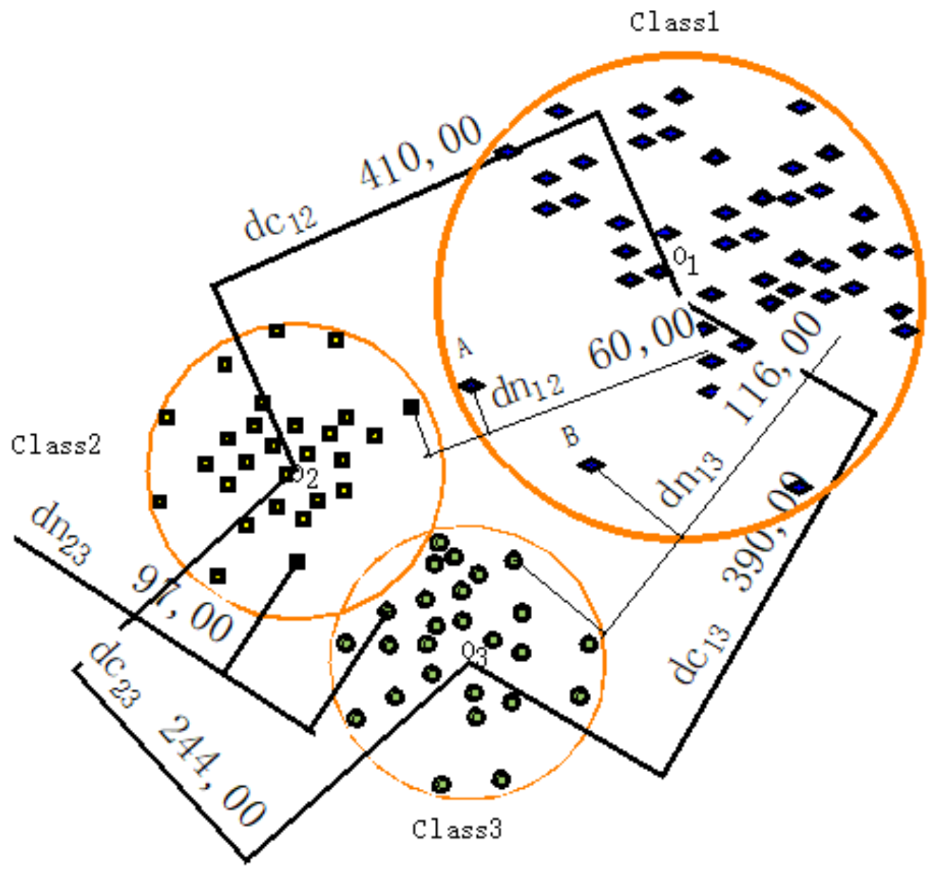
Assuming there are three types of sample signals, one of which has two interference points for points A and B. The two-dimensional spatial distribution of the three types of sample signals is presented in Figure 4. In Figure 4, dc₁₂ is the Euclidean distance between the center of class 1 and class 2, dc₁₃ is the Euclidean distance between the center of class 1 and class 3, dc₂₃ is the Euclidean distance between the center of class 2 and class 3, dn₁₁ is the Euclidean distance between the nearest sample vector of class 1 and class 2, dn₁₃ is the Euclidean distance between the nearest sample vector of class 1 and class 3 and dn₂₃ is the Euclidean distances between the nearest sample vector of class 2 and class 3.

As can be seen in Figure 4, dc₁₂ > dc₁₃ > dc₂₃ and dn₁₃ > dn₂₃ > dn₁₂ can be obtained and class 1 is the easiest to be separated. Due to dc₁₂ > dc₁₃ > dc₂₃ and dn₁₃ > dn₂₃ > dn₁₂ presented in Figure 4, it can be stated that dc₁₂ + dc₁₃ > dc₁₂ + dc₂₃ > dc₁₃ + dc₂₃ and dn₁₃ + dn₂₃ > dn₁₃ + dn₁₂ > dn₁₂ + dn₂₃. Therefore, class 1 is the easiest to be separated by using the sum of the Euclidean distances between the class centers. Whereas, it can be concluded that class 3 is the easiest to be separated by using the sum of the Euclidean distances between the nearest sample vectors between the classes. The result obtained by the sum of the Euclidean distances between the class centers is consistent with what can be seen in reality. It shows that the ISDTSVM algorithm can overcome the influence of the interference points by calculating the Euclidean distances between the class centers.

The procedure of performing the ISDTSVM algorithm is described as follows:

Step 1

According to Equation 6, the center of the classes is obtained, labeli = 0.

Step 2

Calculating the Euclidean distances between the class centers. $d_{ij}$ ($i,j=1,2,\cdots ,k$) are obtained by Equation (7) and a symmetric matrix $D_{k\times k}$ is obtained as well.

Step 3

According to Equation (8), $Sumd(i)$, the sums of the Euclidean distances between classes are obtained by calculating the sum of each row in a symmetric matrix $D_{k\times k}$.

Step 4

Sorting the $Sumd(i)$, labeli = labeli + 1. The class label with maximum $Sumd(i)$ is for the labeli. Elements of line $i$ and column $i$ of $D_{k\times k}$ is assigned to be zero. $k=k-1$, repeating Step 3 to Step 4 until labeli = k.

Step 5

Multi-class classification is conducted using the conventional Skewness Decision Tree SVM.

3. Inertia Weight PSO Algorithm

Let us assume that a population is composed by $m$ particles in D dimension space and a particle is viewed as a point in the D dimension space, representing a solution described by its position and speed. The position of the ith particle can be expressed as $X_i=[X_{i1},X_{i2},\cdots ,X_{{}_{iD}}]$, $i=1,2,\cdots ,m$. The speed can be expressed as $V_i=[V_{i1},V_{i2},\cdots ,V_{iD}]$. The optimal position of ith particle can be expressed as $P_i=[P_{i1},P_{i2},\cdots ,P_{iD}]$. The optimal position of the entire population can be expressed as $P_g=[P_{g1},P_{g2},\cdots ,P_{gD}]$. For the tth iteration, the position and speed of each particle can be updated by Equation (9):

$$\{\begin{array}{l}{V}_{id}^{t+1}={\omega }^t\cdot V_{id}^t+c_1\cdot rand\cdot (P_{id}^t-X_{id}^t)+c_2\cdot rand\cdot (P_{gd}^t-X_{id}^t)\hfill \\ X_{id}^{t+1}=X_{id}^t+V_{id}^{t+1}, d=1,2,\cdots ,D\hfill \end{array}$$

(9)

Equation (9) is so-called as the basic PSO, where t is the number of iterations $\omega$ is the inertia weight coefficient, $c_1$ and $c_2$ are the acceleration constant, the values are generally selected as $c_1=1.5,c_2=1.7$, $rand$ is the random number falling within a normal distribution in [0, 1], $V_{id}$ is the current speed of ith particle and $V_{id}\in [-V_{\max },V_{\max }]$, where $V_{\max }$ is the maximum speed limit. When $V_{id}>V_{\max }$, taking $V_{id}=V_{\max }$; when $V_{id}<-V_{\max }$, taking $V_{id}=-V_{\max }$. The iteration termination criteria of the PSO algorithm is usually given by that the number of iterations reaching to the maximum limit or the tolerance that is less than a specified required value.

The global and local search ability of the particle can be adjusted by changing the size of $\omega$. The larger the $\omega$ value, the stronger the global search ability. On the other hand, it has a stronger local search ability, as its dynamic weight has a better optimization ability than a fixed one. Therefore, the linear decrease dynamic inertia weight strategy is employed. Its formula is given by the Equation (10):

$${\omega }^t={\omega }_{\max }-\frac{{\omega }_{\max }-{\omega }_{\min }}{t_{\max }}\times t$$

(10)

where ${\omega }_{\max }$ and ${\omega }_{\min }$ are the maximum and minimum values respectively, generally ${\omega }_{\max }=0.9$, ${\omega }_{\min }=0.4$. Inertia weight $\omega$ will increase with the number of iterations, as indicated in Equation (10) from the initial value ${\omega }_{\max }$ gradient to ${\omega }_{\min }$ linearly; $t$ and $t_{\max }$ are the current iteration number and the maximum number of iterations.

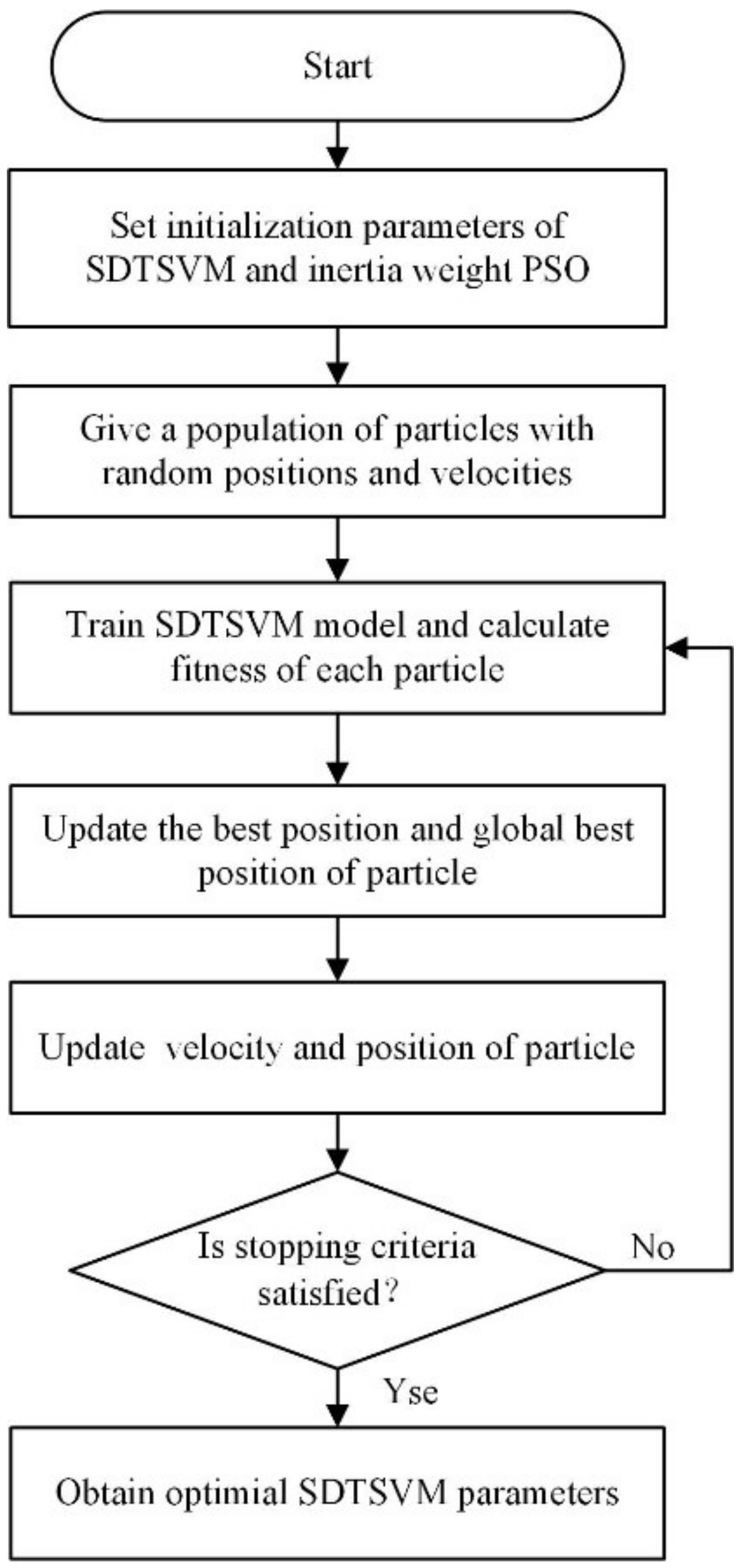
4. ISDTSVM Coupled with an Inertia Weight PSO Algorithm

For the ISDTSVM coupled with Inertia Weight PSO algorithm, the parameter optimization process is presented in Figure 5. The initialization parameters of ISDTSVM and the PSO algorithm, by several test evaluations are as follows: the range of $C$ is 0~100, the range of $\gamma$ is 0~10, the maximum iteration number is 200, the swarm size population number is 20 and ${\omega }_{\max }=0.9$, ${\omega }_{\min }=0.4$and$c_1=1.5,c_2=1.7$.

The initial position and speed of the particle are randomly generated. The fitness function is based on a classification accuracy of the ISDTSVM trained with the data subset. In the five-fold cross-validation, the data set is divided into five data subsets. The position and speed of each particle can be updated by the Equation (9). The iteration termination criteria of the PSO algorithm was given by the number of iterations that reached the maximum iteration number.

5. Experimental Results and Discussion

5.1. Experimental Results of the UCI Datasets

The proposed ISDTSVM algorithm was used for the classification of the multi-class UCI data sets. The features of the multi-class UCI data sets are presented in

Table 1. The features of the University of California Irvine (UCI) data sets.

UCI Data Sets	Samples	Number of Attributes	Data Categories
Vowel	528	10	11
Zoo	104	17	7
Wine	178	13	3

The optimized results of the SVM parameters $C$ and $\gamma$ (replaced by the letter: g) based on the UCI data sets using an inertial weight PSO algorithm are presented in Figure 6.

.

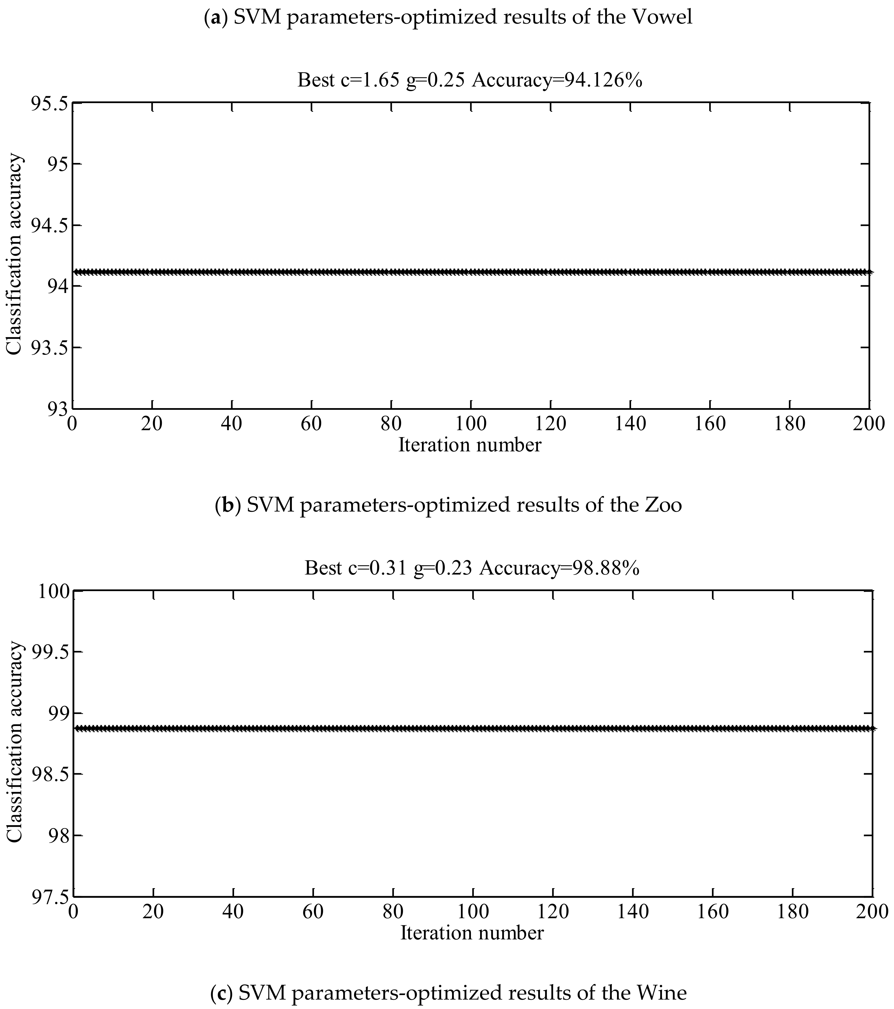
Accuracy of the k-fold cross-validation was taken in to account as a criterion to evaluate the effectiveness of a classification algorithm. The five-fold cross-validation were carried out. The classification testing results of the UCI data sets are presented in

Table 2. The classification results of the UCI data sets using the Improved Skewness Decision Tree Support Vector Machine (ISDTSVM) and the conventional Skewness Decision Tree Support Vector Machine (SDTSVM) algorithm with different kernel functions and a five-fold cross-validation.

UCI Data Sets	Kernel Functions	Average Accuracy of Conventional SDTSVM	Average Accuracy of ISDTSVM	Classification Order of ISDTSVM
Vowel	Radial basis function ($C$ = 4.81, $\gamma$ = 0.86)	96%	99%	1→8→10→2→3→9→7→5→4→6→11
Vowel	Polynomial (d = 3)	95%	97%
Zoo	Radial basis function ($C$ = 1.65, $\gamma$ = 0.25)	95%	98%	6→4→1→2→3 →5→7
Zoo	Polynomial (d = 1)	93%	96%
Wine	Radial basis function ($C$ = 0.31, $\gamma$ = 0.23)	97%	98%	3→1→2
Wine	Polynomial (d = 2)	97%	97%

by using the ISDTSVM algorithm and the conventional SDTSVM algorithm with optimized parameters (Figure 6) and two kinds of kernel functions. As can be observed, for the Vowel, Zoo and Wine data sets, the ISDTSVM algorithm improves the average classification accuracy by 3%, 3% and 1% respectively. The classification accuracy of the radial basis function kernel was higher than the polynomial kernel. The classification results of the Wine data sets are presented in

Table 3. Classification results of the Wine data sets for the three classification orders using the SDTSVM algorithm with a radial basis function and a five-fold cross-validation.

Classification Order	Kernel Functions	Average Accuracy of SDTSVM
1→2→3	Radial basis function ($C$ = 0.31, $\gamma$ = 0.23)	97%
2→1→3	Radial basis function ($C$ = 0.31, $\gamma$ = 0.23)	97%
3→1→2	Radial basis function ($C$ = 0.31, $\gamma$ = 0.23)	98%

using the SDTSVM algorithm with all of the possible classification orders and radial basis function kernel. As can be observed, the determined classification order by the ISDTSVM algorithm has the highest classification accuracy.

5.2. Experimental Results of Steel Cord Conveyor Belt Defects

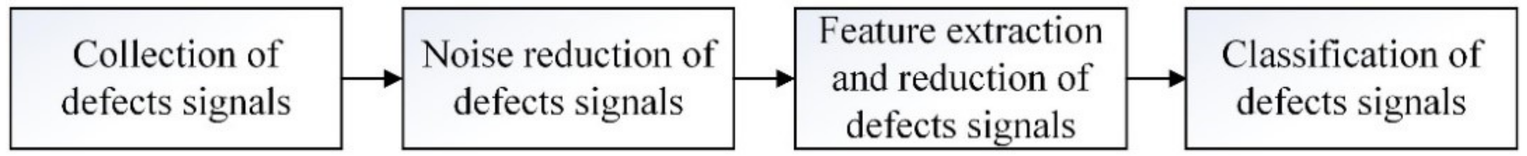
The typical defects of the steel cord conveyor belt include a splice twitch, broken rope and rope fatigue. Splice signals identification is the basis for quantitative detection of the splice twitch. Therefore, the splice signals were identified as a defect signal. The proposed ISDTSVM algorithm with inertia weight PSO algorithm was applied to the classification of steel cord conveyor belt defects. The diagnosis procedure flow chart of steel cord conveyor belt defects is presented in Figure 7. The key steps were noise reduction, feature extraction and classification of defects signals.

5.2.1. Collection of the Defects Signals

The scheme of the weak magnetic signals collection experiment platform is presented in Figure 8. First, the weak magnetic loading module was installed to magnetize the wire rope in the steel cord conveyor belt. Then, the operating velocity of the belt was 0.5 m/s. The signals were collected by the weak magnetic testing device and transmitted to the upper computer by the TCP/IP protocol, as presented in Figure 9. The main parameters of the weak magnetic testing device were defined. More specifically, the sensitivity of the sensor was 0.5 V/Gs, the sample interval was 0.0005 mm and the data transmission rate was 100 Mbps.

5.2.2. Noise Reduction and Normalization of the Defects Signals

Weak magnetic signals of the steel cord conveyor belt defects could easily be disturbed by strong and non-stationary noise in coal mine. Therefore, the noise of the defects signals was reduced using a noise reduction method, combining the wavelet packet and the RLS (Recursive Least Squares) adaptive filtering [24]. The noise reduction principle of the filtering algorithm is presented in Figure 10. $x(n)$ was the input signal that includes the useful signal $s(n)$ and the noise signal $N_1(n)$. The sum of the multi-layer high frequency detail signal for $\mathrm{x}(n)$ was decomposed by the wavelet packet. $N_2(n)$ was used as the noise reference signal of the RLS adaptive filter algorithm. Finally, the noise of the defect signals were reduced by the RLS adaptive filtering algorithm.

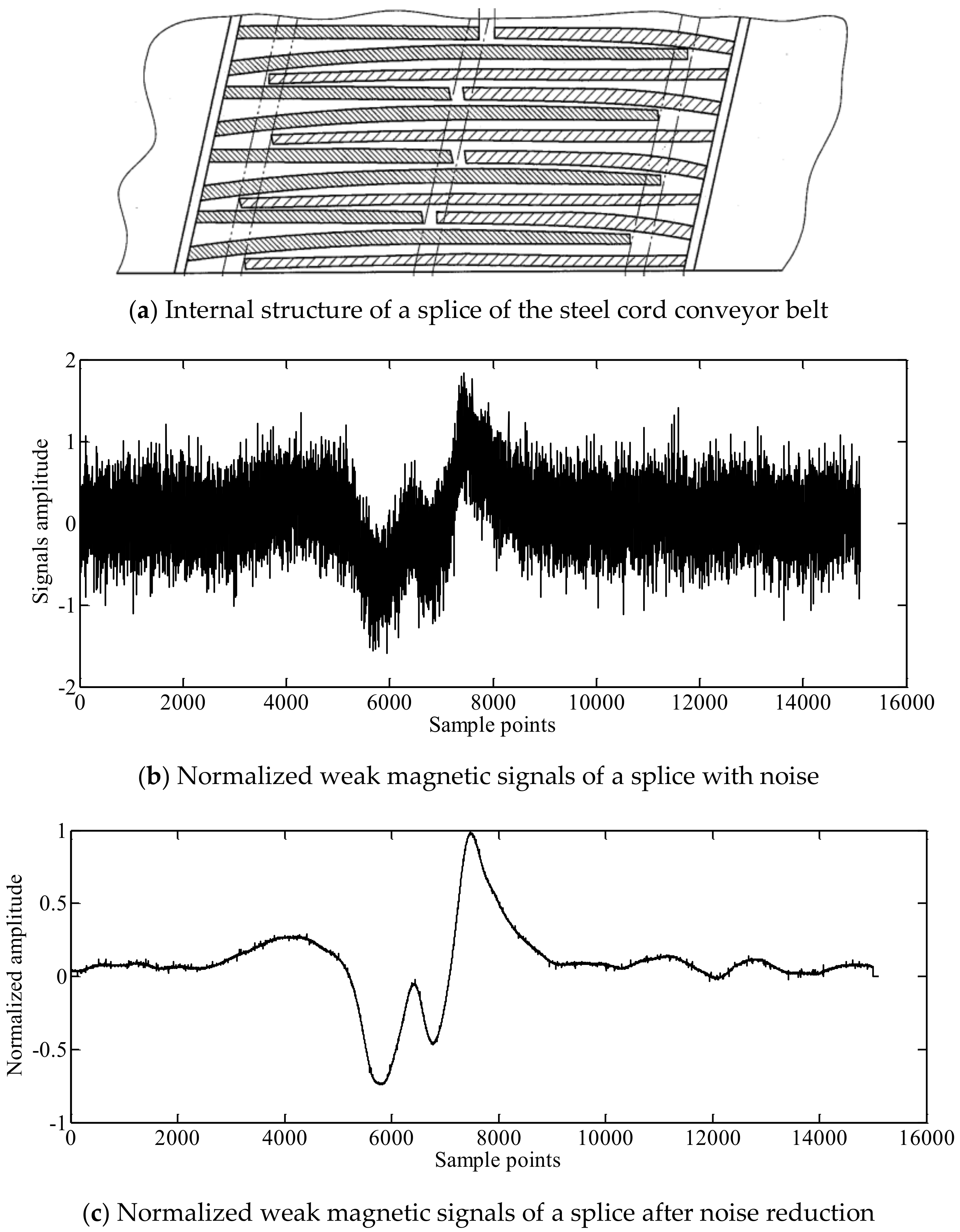
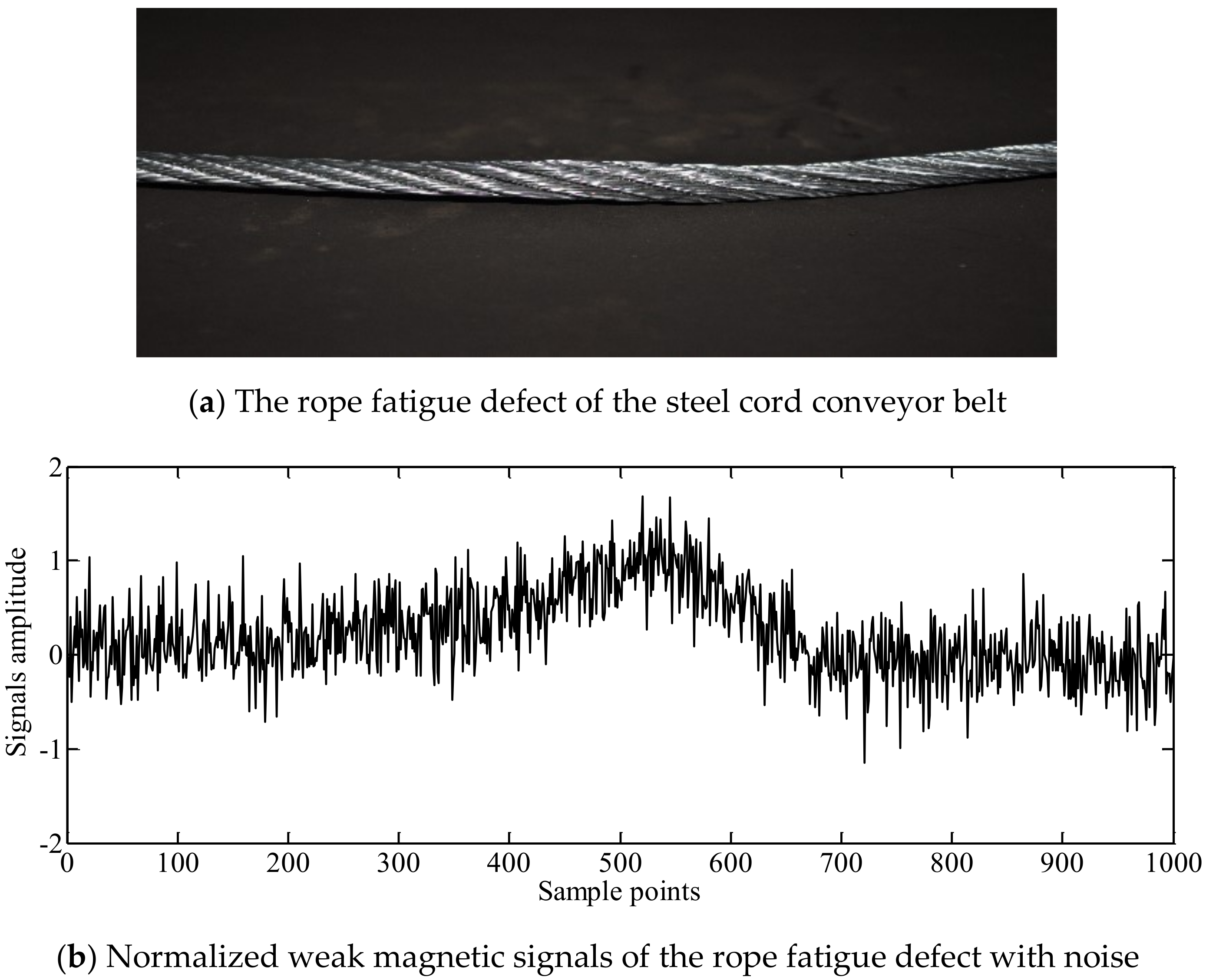
In order to eliminate the effect of the signals amplitude on classification, the signals after noise reduction were normalized. The normalized signals of the splice, the broken rope defect and the rope fatigue defect before and after noise reduction are presented in Figure 11, Figure 12 and Figure 13.

5.2.3. Feature Extraction and Reduction of the Defects Signals

The frequency domain and time domain features of the weak magnetic signals of the steel cord conveyor belt defects were extracted. The spectral amplitudes corresponding to the different defects are presented in Figure 14. The peaks are observed at similar frequencies, with slight discrepancies at the amplitude. Therefore, the time domain features are selected for the classification.

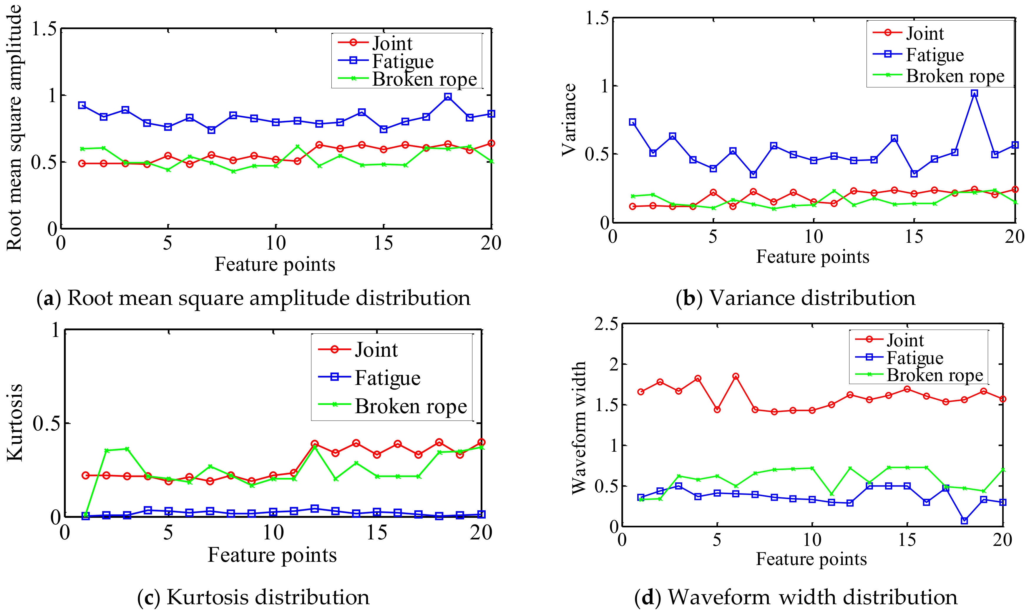
First, twelve common time domain fault features were extracted, which were the peak-to-peak values, root mean square amplitudes, mean amplitudes, variance, root amplitudes, waveform width, kurtosis, wave index, peak index, pulse index, margin index and the kurtosis index. Then, the features were reduced by a neighborhood rough set algorithm. The four time domain features, after reduction were root mean square amplitudes, variance, kurtosis and waveform width. The root mean square amplitudes mainly reflected the signals energy, the variance mainly reflected the degree of the signals dispersion and the kurtosis mainly reflected signal sharpness and impact characteristics. As can be observed in Figure 11, Figure 12 and Figure 13, the normalized signal features of the splice, broken rope defect and rope fatigue defect were significantly different in waveform width, signals energy, degree of signals dispersion, signal sharpness and impact, the waveform width and kurtosis of splice signals were usually larger than the broken rope defect and the rope fatigue defect. Therefore, according to the features reduction and waveform analysis in Figure 11, Figure 12 and Figure 13, the four domain features, finally determined, were root mean square amplitude, variance, kurtosis and waveform width.

For a given the sample signals $x_i$ and the number N, the four time domain features calculation expressions are presented as follows:

(1) Root Mean Square Amplitude (RMSA)

$$X_{rms}=\sqrt{\frac{1}{N}{\displaystyle \sum _{i=1}^N{x}_i{}^2}}$$

(11)

(2) Variance

$${\sigma }_x=\frac{1}{N}{\displaystyle \sum _{i=1}^N{(x_i-\overline{x})}^2}$$

(12)

where $\overline{x}$ is the average value of $x_i$.

(3) Kurtosis

$$\beta =\frac{1}{N}{\displaystyle \sum _{i=1}^N{x}_i{}^4}$$

(13)

(4) Waveform width

Given the position number N_r5 for the first raising edge at 5% of the maximum value of $\left|x_i\right|$ and the position number N_f5 for the last falling edge at 5% of the maximum value of $\left|x_i\right|$. The collection interval d_ci was 0.0005 mm. The waveform width P_wide was given by Equation (14).

P_wide = (N_f5 − N_r5 ) × d_ci

(14)

The distributions of the four time domain features of the partial sample signals are presented in Figure 15. As can be seen in Figure 15, the four time domain features distribution results of the splices, broken rope defects and the rope fatigue defects were significantly different, which was consistent with the features reduction and waveform analyses (Figure 11, Figure 12 and Figure 13). As can be observed in Figure 15, the splice could be identified well by the waveform width and the rope fatigue could be identified well by the other three features. However, according to the splice structure, rope fatigue and broken rope defects presented in Figure 11a, Figure 12a and Figure 13a, the length of the splice, fracture width of broken rope defect and the fatigue length of the rope fatigue defect could lead to changes of the waveform width. It may cause overlapping waveform width distribution for three types of weak magnetic signals in actual operating conditions. Therefore, in order to improve the classification accuracy of the steel cord conveyor belt in actual working conditions, four time domain features were used together for classification.

5.2.4. Classification of the Defects Signals

One hundred and sixty-eight sample feature vectors of the normalized signals for the steel cord conveyor belt defects, were obtained. The sample sets were composed by seventy-four sample feature vectors of splices, twenty sample feature vectors of the rope fatigue defects and seventy-four samples feature vectors of the broken rope defects. That is that the samples size is imbalanced. The detailed parameter configuration of the inertia weight PSO algorithm was as follows: The range of $C$ was 0~100, the range of$\gamma$was 0~10, the maximum iteration number was 200, the initial population number was 20 and ${\omega }_{\max }=0.9$, ${\omega }_{\min }=0.4$ and $c_1=1.5,c_2=1.7$. The SVM parameters$C$and$\gamma$were optimized using the inertial weight PSO algorithm under an imbalanced samples condition and the corresponding results of the steel cord conveyor belt defects signals are presented in Figure 16.

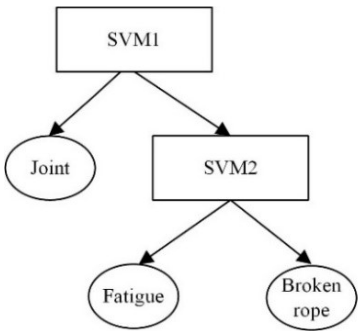
Classification results of the steel cord conveyor belt defects using the ISDTSVM algorithm and the conventional SDTSVM algorithm with different kernel functions and five-fold cross-validation are presented in

Table 4. Classification results of the steel cord conveyor belt defects signals using the ISDTSVM and the conventional SDTSVM algorithm with different kernel functions and five-fold cross-validation.

Kernel Functions	Average Accuracy of Conventional SDTSVM	Average Accuracy of ISDTSVM
Radial basis function ($C$ = 26.64, $\gamma$ = 0.97)	90%	94%
Polynomial (d = 4)	89%	92%

. As can be observed, the ISDTSVM algorithm improved the classification accuracy of the steel cord conveyor belt defect signals by 4%. The classification accuracy of the radial basis function kernel was higher than the polynomial kernel. The tree structure was obtained in Figure 17 using the ISDTSVM algorithm. In order to verify the classification effect of the ISDTSVM algorithm, the classification results for the three classification orders of the steel cord conveyor belt defect signals are presented in

Table 5. Classification results of the steel cord conveyor belt defects signals for three classification orders using the SDTSVM algorithm with a radial basis function kernel and a five-fold cross-validation.

Classification Order	Average Accuracy of SDTSVM
Splice→Rope fatigue→Broken rope (determined by ISDTSVM algorithm)	94%
Rope fatigue→Splice→Broken rope	90%
Broken rope→Splice→Rope fatigue	91%

using the SDTSVM algorithm with optimized parameters presented in Figure 16 and were validated by a five-fold cross-validation. As can be observed in Table 5, the classification accuracy of the classification order obtained by the ISDTSVM algorithm was the highest in the three classification orders. The ISDTSVM algorithm significantly improved the classification accuracy.

5.3. Discussions

Regarding the problem of the classification accuracy of the SDTSVM algorithm being highly dependent on the parameters and the classification order, an improved SDTSVM algorithm was proposed. In the proposed model, the classification order of the ISDTSVM algorithm was determined by the sum of the Euclidean distances between the multi-class samples centers and the parameters were optimized by the inertia weight PSO algorithm.

As presented in Figure 6 and Figure 16, the classification accuracy of the trained data sets was higher than 94% for the UCI data sets and the steel cord conveyor belt defects signals using the inertia weight PSO algorithm. As presented in Table 2 and Table 4, for the Vowel, the Zoo and the Wine data sets, as well as the steel cord conveyor belt defects, the ISDTSVM algorithm improved the classification accuracy by 3%, 3%, 1% and 4% respectively, compared to the conventional SDTSVM algorithm.

In order to verify the impact of the imbalanced samples on the classification of the steel cord conveyor belt defects, experimentation was performed on the steel cord conveyor belt defects samples with a different imbalanced ratio (IR) [25]. The positive class was chosen for the fewest samples and the rest of the samples was a negative class. For the imbalanced classes classification evaluation, metrics such as accuracy, balanced accuracy and F1 were used [26]. A half of the samples were used for training and the other half of samples were used for testing. The steel cord conveyor belt defects samples with the different imbalanced ratio (IR) were classified using the ISDTSVM algorithm and the corresponding results are presented in

Table 6. The classification contrast results of the steel cord conveyor belt defects with different imbalanced ratio using the ISDTSVM algorithm.

Data Sets	Number of Three Types of Samples	IR	Accuracy	Balanced Accuracy	F1
Steel cord conveyor belt defects	20,20,20	2	97%	98%	95%
Steel cord conveyor belt defects	74,20,74	7.4	94%	97%	80%

. As can be observed, the lower IR samples had a higher accuracy, balanced accuracy and F1. The results showed that the imbalanced samples could decrease the classification accuracy of the ISDTSVM algorithm.

On the whole, the SVM parameter $C$ and $\gamma$ could be optimized well using the inertia weight PSO algorithm and the optimal classification order could be determined by the sum of the Euclidean distances between the multi-class samples centers in the ISDTSVM algorithm. The ISDTSVM algorithm could efficiently improve the classification accuracy of the steel cord conveyor belt defects. It was noted that the imbalanced samples could reduce the classification accuracy when using the ISDTSVM algorithm. The ISDTSVM algorithm is recommended for further improvements, when there are imbalanced data sets.

6. Conclusions

In this study, we proposed an ISDTSVM algorithm. Compared to the conventional SDTSVM algorithm, the classification order was determined by the sum of the Euclidean distances between the multi-class sample centers and the parameters were optimized by the inertia weight PSO algorithm. Experiments were conducted on the multi-class UCI data sets and the steel cord conveyor belt defects signals using the ISDTSVM algorithm and the conventional SDTSVM algorithm. For the Vowel, the Zoo and the Wine data sets, as well as the steel cord conveyor belt defects, the ISDTSVM algorithm improved the classification accuracy by 3%, 3%, 1% and 4% respectively, compared to the conventional SDTSVM algorithm. The classification accuracy of the steel cord conveyor belt defects reached 94% using the proposed ISDTSVM algorithm. The experiment results showed that the inertia weight PSO algorithm could optimize the SVM parameters quite well and the proposed ISDTSVM algorithm could improve the classification accuracy significantly. It could be applied efficiently to the classification of the steel cord conveyor belt defects. It has an important significance for preventing fracture accidents of steel cord conveyor belts.

Compared to the conventional SDTSVM algorithm, although the proposed ISDTSVM algorithm could improve the classification accuracy by considering the distribution characteristics of the samples. The algorithm has limitations for outliers, noise and imbalanced data sets. In the future, we will study the ISDTSVM algorithm combined with the FSVM algorithm and how the algorithm works for imbalanced data sets.

References

- Fedorko, G.; Molnár, V.; Ferková, Ž.; Peterka, P.; Krešák, J.; Tomašková, M. Possibilities of failure analysis for steel cord conveyor belts using knowledge obtained from non-destructive testing of steel ropes. Eng. Fail. Anal. 2016, 67, 33–45. [Google Scholar] [CrossRef]
- Błażej, R.; Jurdziak, L.; Kozłowski, T.; Kirjanów, A. The use of magnetic sensors in monitoring the condition of the core in steel cord conveyor belts–Tests of the measuring probe and the design of the DiagBelt system. Measurement 2018, 123, 48–53. [Google Scholar]
- Tharwat, A.; Hassanien, A.E.; Elnaghi, B.E. A BA-based algorithm for parameter optimization of Support Vector Machine. Pattern Recognit. Lett. 2017, 93, 13–22. [Google Scholar] [CrossRef]
- Beltrami, M. Grid-Quadtree Algorithm for Support Vector Classification Parameters Selection. Appl. Math. Sci. 2015, 9, 75–82. [Google Scholar] [CrossRef]
- Phan, A.V.; Nguyen, M.L.; Bui, L.T. Feature weighting and SVM parameters optimization basedon genetic algorithms for classification problems. Appl. Intell. 2017, 46, 455–469. [Google Scholar] [CrossRef]
- Qian, R.; Wu, Y.; Duan, X. SVM Multi-Classification Optimization Research based on Multi-Chromosome Genetic Algorithm. Int. J. Perform. Eng. 2018, 14, 631–638. [Google Scholar] [CrossRef]
- Venkateswaran, K.; Sowmya Shree, T.; Kousika, N.; Kasthuri, N. Performance Analysis of GA and PSO based Feature Selection Techniques for Improving Classification Accuracy in Remote Sensing Images. Indian J. Sci. Technol. 2016, 9, 1–7. [Google Scholar] [CrossRef]
- Alba, E.; Garcia-Nieto, J.; Jourdan, L.; Talbi, E.-G. Gene Selection in Cancer Classification using PSO/SVM and GA/SVM Hybrid Algorithms. In Proceedings of the 2007 IEEE Congress on Evolutionary Computation, Singapore, 25–28 September 2007. [Google Scholar]
- Liu, Z.W.; Cao, H.R.; Chen, X.F.; He, Z.; Shen, Z. Multi-fault Classification Based on Wavelet SVM with PSO Algorithm to Analyze Vibration Signals from Rolling Element Bearings. Neurocomputing 2013, 99, 399–410. [Google Scholar] [CrossRef]
- Mohammadi, J.A.; Davar, G. Automatic Detection of Erythemato-squamous Diseases Using PSO–SVM Based on Association Rules. Eng. Appl. Artif. Intell. 2013, 26, 603–608. [Google Scholar]
- Harrison, K.R.; Engelbrecht, A.P.; Ombuki-Berman, B.M. Inertia weight control strategies for particle swarm optimization. Swarm Intell. 2016, 10, 267–305. [Google Scholar] [CrossRef]
- Tomar, D.; Agarwal, S. A comparison on multi-class classification methods based on least squares support vector machine. Knowl.-Based Syst. 2015, 81, 131–147. [Google Scholar] [CrossRef]
- Chen, Y.; Ma, H.-W.; Zhang, G.-M. A support vector machine approach for classification of welding defects from ultrasonic signals. J. Nondestruct. Test. Eval. 2014, 29, 243–254. [Google Scholar] [CrossRef]
- Wang, S.; Li, Y.; Shao, Y.; Carlo, C.; Zhang, Y.; Du, S. Detection of Dendritic Spines Using Wavelet Packet Entropy and Fuzzy Support Vector Machine. CNS Neurol. Disord.–Drug Targ. 2017, 16, 116–121. [Google Scholar] [CrossRef] [PubMed]
- Zhang, Y.; Yang, Z.; Lu, H.; Zhou, X.; Phillips, P.; Liu, Q.; Wang, S. Facial Emotion Recognition Based on Biorthogonal Wavelet Entropy, Fuzzy Support Vector Machine, and Stratified Cross Validation. IEEE Access 2016, 4, 8375–8385. [Google Scholar] [CrossRef]
- Muthanantha, A.S.; Ramakrishnan, M.S. Hierarchical multi-class SVM with ELM kernel for epileptic EEG signal classification. Med. Biol. Eng. Comput. 2016, 54, 149–161. [Google Scholar]
- Xue, Y.; Ju, Z.; Xiang, K.; Chen, J.; Liu, H. Multiple Sensors Based Hand Motion Recognition Using Adaptive Directed Acyclic Graph. Appl. Sci. 2017, 7, 1–14. [Google Scholar] [CrossRef]
- Lajnef, T.; Chaibi, S.; Ruby, P.; Aguera, P.-E.; Eichenlaub, J.-B.; Samet, M.; Kachouri, A.; Jerbi, K. Learning machines and sleeping brains: Automatic sleep stage classification using decision-tree multi-class support vector machine. J. Neurosci. Methods 2015, 250, 94–105. [Google Scholar] [CrossRef]
- Zhang, Y.; Wang, S.; Dong, Z. Classification of Alzheimer Disease Based on Structural Magnetic Resonance Imaging by Kernel Support Vector Machine Decision Tree. Prog. Electromagn. Res. 2014, 144, 171–184. [Google Scholar] [CrossRef]
- Takahashi, F.; Abe, S. Decision-tree-based multiclass support vector machines. In Proceedings of the 9th International Conference, Seoul, Korea, 5–7 August 2002; 3, pp. 1418–1422. [Google Scholar]
- Xu, Z.; Li, P.; Wang, Y. Text Classifier Based on an Improved SVM Decision Tree. Phys. Procedia 2012, 33, 1986–1991. [Google Scholar] [CrossRef]
- Vapnik, V.N. Statistical Learning Theory; PHEI: Beijing, China, 2009. [Google Scholar]
- Fuchida, M.; Pathmakumar, T.; Mohan, R.E.; Tan, N.; Nakamura, A. Vision-Based Perception and Classification of Mosquitoes Using Support Vector Machine. Appl. Sci. 2017, 7, 1–12. [Google Scholar] [CrossRef]
- Mao, Q.; Ma, H.; Zhang, X. Steel Cord Conveyor Belt Defect signal Noise Reduction Method Based on a Combination of Wavelet Packet and RLS Adaptive Filtering. In Proceedings of the 2016 International Symposium on Computer, Consumer and Control (IS3C), Xi’an, China, 4–6 July 2016. [Google Scholar]
- Gonzalez-Abril, L.; Nu˜nez, H.; Angulo, C.; Velasco, F. GSVM: An SVM for handling imbalanced accuracy between classes inbi-classification problems. Appl. Soft Comput. 2014, 17, 23–31. [Google Scholar] [CrossRef]
- Lin, Z.; Hao, Z.; Yang, X. Effects of Several Evaluation Metrics on Imbalanced Data Learning. J. South China Univ. Technol. 2010, 38, 147–155. [Google Scholar]
Figure 1.
The structure of the steel cord conveyor belt.
Figure 2.
A photo of the steel cord conveyor belt after a fracture failure.
Figure 3.
Illustration of the conventional Skewness Decision Tree Support Vector Machine (SVM).
Figure 4.
Two-dimensional spatial distribution of the three types of sample signals.
Figure 5.
The SVM parameter optimization process using an inertia weight Particle Swarm Optimization (PSO) algorithm.
Figure 6.
SVM parameters optimized results of the UCI data sets.
Figure 7.
Diagnosis procedure flow chart of the steel cord conveyor belt defects signals.
Figure 8.
Scheme of the weak magnetic signals collection experiment platform.
Figure 9.
Installing picture of the weak magnetic testing device
Figure 10.
Noise reduction principle for a combination of the wavelet packet and the Recursive Least Squares (RLS) adaptive filter.
Figure 11.
Normalized weak magnetic signals of a splice before and after noise reduction.
Figure 12.
Normalized weak magnetic signals of the broken rope defect before and after noise reduction.
Figure 13.
Normalized weak magnetic signals of the rope fatigue defect before and after noise reduction.
Figure 14.
Amplitude spectrum for the weak magnetic signals of the steel cord conveyor belt defects.
Figure 15.
Features distribution for three types of normalized weak magnetic signals.
Figure 16.
Parameter optimal results under the unbalanced samples condition.
Figure 17.
The tree structure obtained by the ISDTSVM algorithm.