Abstract
There is increasing interdisciplinary interest in phytoplankton community dynamics as the growing environmental problems of water quality (particularly eutrophication) and climate change demand attention. This has led to a pressing need for improved biophysical and causal understanding of Phytoplankton Functional Type (PFT) optical signals, in order for satellite radiometry to be used to detect ecologically relevant phytoplankton assemblage changes. Biophysically and biogeochemically consistent phytoplankton Inherent Optical Property (IOP) models play an important role in achieving this understanding, as the optical effects of phytoplankton assemblage changes can be examined systematically in relation to the bulk optical water-leaving signal. The Equivalent Algal Populations (EAP) model is used here to investigate the source and magnitude of size- and pigment- driven PFT signals in the water-leaving reflectance, as well as the potential to detect these using satellite radiometry. This model places emphasis on the determination of biophysically consistent phytoplankton IOPs, with both absorption and scattering determined by mathematically cogent relationships to the particle complex refractive indices. All IOPs are integrated over an entire size distribution. A distinctive attribute is the model’s comprehensive handling of the spectral and angular character of phytoplankton scattering. Selected case studies and sensitivity analyses reveal that phytoplankton spectral scattering is most useful and the least ambiguous driver of the PFT signal. Key findings are that there is the most sensitivity in phytoplankton backscatter () in the 1–6 m size range; the backscattering-driven signal in the 520 to 570 nm region is the critical PFT identifier at marginal biomass, and that, while PFT information does appear at blue wavelengths, absorption-driven signals are compromised by ambiguity due to biomass and non-algal absorption. Low signal in the red, due primarily to absorption by water, inhibits PFT detection here. The study highlights the need to quantitatively understand the constraints imposed by phytoplankton biomass and the IOP budget on the assemblage-related signal. A proportional phytoplankton contribution of approximately 40% to the total appears to a reasonable minimum threshold in terms of yielding a detectable optical change in . We hope these findings will provide considerable insight into the next generation of PFT algorithms.
1. Introduction
Phytoplankton across the world’s oceans represent about half of all primary production on our planet [1,2]. Their growth and function are fundamental to sustaining life: they constitute the foundation of the aquatic food web, and serve critical roles in the recycling of essential elements such as carbon and nitrogen, as well as in remineralisation [3,4,5]. Being so responsive to nutrient availability and water temperature, these tiny organisms are key indicators of ecosystem change, and understanding their community dynamics is key to answering some of the most challenging earth science questions of our time about the impacts of climate change on local, regional and global scale aquatic systems and the carbon cycle. The widespread distribution and integral role of phytoplankton in global marine ecosystems means that these fields of study depend heavily on modelling together with satellite data for any large scale analysis. In situ data collection is indispensable for local scale investigations and for ground truthing of satellite and model data, but simultaneous large scale direct measurements are logistically impossible. Optical measurements in natural waters are challenging: they are expensive and logistically difficult, technically complex due to large dynamic ranges of the signal, and overall require delicate, rigorously calibrated instrumentation with precise knowledge of sources of error. Remote sensing and moored in situ instrumentation are the only feasible ways to acquire continuous data series, but these largely involve bulk measurements of the total optical signal. Isolating the respective optical components for laboratory assessment is a significant further undertaking. In situ and laboratory measurements are consequently extremely valuable, and appropriate bio-optical models provide essential tools for the analysis and understanding of these bulk measurements, whether above- or sub-surface.
It has long been appreciated that phytoplankton have a direct effect on the observable colour of the ocean, and broad scale biomass estimates based on Chl a concentrations derived from satellite radiometry are widely relied upon despite persistent uncertainty in the accuracy of information derived from satellite imagery [6,7]. Recently, there has been considerable interest in more detailed information on phytoplankton assemblage characteristics [8,9,10,11], but it has not been widely ascertained to what degree Phytoplankton Functional Type (PFT) information can be gleaned from satellite data, and at what level of confidence. Furthermore, descriptions of PFTs differ with context—and the potential for identifying relationships between the ecological roles of phytoplankton and their optical properties must also be considered. Understanding the causal effect of biophysical phytoplankton characteristics on the optical water-leaving signal is at the heart of addressing these questions, and this is undoubtedly an outstanding topic in ocean optics.
Any useable radiometric PFT-related signal results directly from the interaction of phytoplankton with their light environment, but the physical basis of this interaction is not well understood in terms of observed variability across the wide diversity of aquatic environments and phytoplankton assemblages [12,13]. Generally, in oceanic waters, it is the strong absorption by phytoplankton which dominates the phytoplankton contribution to the ocean colour signature, and has therefore been identified as a promising signal in terms of PFT identification. However, distinguishing the effects of variable phytoplankton absorption due to biomass changes from the effects due to functional type changes (and further from changes induced by photoacclimation and photoprotective pigments) is not straightforward. This ambiguity in the phytoplankton community signal is at the core of the PFT problem. It is then overlaid with further complexity, given that a potential PFT signal from the phytoplankton component of a water body’s optical constituents must be considered in the context of the other components in the water, recognising the contributions from the non-algal sources of optical variability: absorption due to CDOM (Coloured Dissolved Organic Matter) and detrital particles, i.e., , and non-algal backscatter i.e., [13]. The blue spectral region of maximum phytoplankton absorption is also the region most affected by CDOM and detrital absorption. (It should also be noted that, in the context of satellite radiometry, blue spectral bands display the largest absolute measurement uncertainties [7,14]. While the blue water-leaving signal may be large in oceanic regions, resulting in a small relative uncertainty, this is when the signal is overwhelmingly dominated by the backscattering of water, decreasing confidence in the lesser contributions of and . Generally, product retrievals from the satellite tend to be less robust than those of other IOPs [15,16].)
A comprehensive guide to PFT approaches is given by Mouw et al. [17], dividing them into four categories: abundance-based e.g., Hirata et al. [18] and Brewin et al. [19,20]; radiance based e.g., the PHYSAT method: Alvain et al. [21,22]; absorption based e.g., Devred et al. [23], Ciotti and Bricaud [24], and PhytoDOAS: Bracher et al. [25]; and scattering based e.g., Kostadinov et al. [10,26] (all references in [17]). Existing scattering-based approaches [10,11] assume a Jungian (exponential) particle size distribution and rely on Mie modelling, which does not adequately represent phytoplankton angular scattering [27], and there are consequently high uncertainties in PSD retrieval where the particle size distribution slope is low, i.e., highly productive and coastal areas dominated by relatively large cells [10]. Low biomass (Chl a < 1 mg·m) oceanic conditions with an absorption-dominated phytoplankton component of the water-leaving signal can exhibit good relationships with differential pigment absorption e.g., the diagnostic pigment approach used on satellite in Uitz et al. [28]. It follows that, in the context of additional non-algal absorption, differentiated spectra show better similarity than non-differentiated [29], and also that high spectral resolution measurements show better potential for retrieving phytoplankton assemblage information than multi-spectral [29] when retrieving diagnostic features of the first derivative of . However, other methods using the fourth derivative of pigment absorption and to identify fine-scale phytoplankton absorption features have found that objective discrimination of pigment groups from hyperspectral may not be feasible at low biomass < 1 mg·m due to the high similarities in the derivative spectra [30]. This suggests that the primary phytoplankton signal in is due to biomass (Chl a) rather than the accessory pigments, and that with the exception of uniquely diagnostic pigment absorption outside the spectral regions of that of Chl a, phytoplankton information cannot be retrieved without assumptions about PFT relationships with biomass. The PhytoDOAS method also employs a fourth derivative analysis [25,31] but is performed on hyperspectral top-of-atmosphere satellite measurements, avoiding the uncertainties associated with poor atmospheric correction, but the sensitivity of this high spectral resolution approach to biomass and both algal and non-algal scattering contributions to the IOP budget has yet to be determined.
Generally, phytoplankton absorption- and abundance-based methods rely on empirical relationships between biomass, functional type and CDOM. Where these quantities co-vary predictably or are exactly known, empirical PFT algorithms may be successful. However, Brewin et al. [6] acknowledges that both the abundance-based approaches as well as approaches relying on differential pigment absorption break down in environments that do not conform to the generalised relationships between community structure and biomass upon which these approaches are based, usually in elevated biomass comprised of small cells. The relative contributions of phytoplankton absorption and scatter to light emerging from seawater change with biomass, size and other functional type traits, and as the and components vary (see Stramski et al. [32] and references therein). The total water-leaving signal is a delicate balance of the frequently opposing optical effects of biomass and phytoplankton assemblage variability such as size, pigments and ultrastructure, together with the optical effects of the non-algal in-water constituents. An interactive webpage demonstrating the first order effect of variability in these parameters on Rrs is available in the Supplementary Material. It was observed by Brown et al. [13] that backscatter anomaly maps (i.e., backscatter independent of variability due to biomass) correlate approximately with PFT distribution maps calculated from optical anomalies which were initially attributed to differences in phytoplankton accessory pigments [21]. This leads to the suggestion that radiance-based methods, e.g., the Alvain (PHYSAT) criteria used to distinguish PFTs, are in fact primarily due to backscattering characteristics [9,13], indicating that phytoplankton groups either directly determine, or perhaps are simply associated with, backscattering variability around the mean.
Brown et al. [13] conclude that these relationships can only be fully explored if a method is applied where the phytoplankton groups are causally linked to the optical conditions. The Equivalent Algal Populations (EAP) model provides exactly such a method, and is used here to investigate the impact of size- and pigment-based PFT variability on the optical signal, and to confirm the assertion that biomass drives the largest part of observed variability in the water-leaving signal, and that the radiometric signal in the blue is ambiguous due to the effects of , and the additional effects of [13,33].
The EAP model is a fully physics-based two-layered spherical model, which calculates, from first principles, biophysically linked phytoplankton absorption and scattering characteristics from particle refractive indices reflecting the primary light-harvesting pigments of various phytoplankton groups. IOPs are calculated at high spectral resolution between 400 and 900 nm and are integrated over an entire equivalent size distribution [34,35], simulating the dominant optical characteristics of natural phytoplankton assemblages. The EAP is used here only as a forward model: the intention of this study is to isolate the biophysical driver(s) of PFT optical signals and determine the associated implications for detecting PFT changes from satellite radiometry.
In this study, the term “Phytoplankton Functional Type” is used in a broad sense of the dominant characteristics of a phytoplankton assemblage, with respect to both cell size and accessory pigments, from an optical perspective.
Study Objectives and Outline
The aim of this work is to investigate the magnitude and spectral location of optical water-leaving signals resulting from phytoplankton assemblage changes; to determine how these signals respond to changes in biomass and functional type; to evaluate their optical ambiguity in the context of the optical effects of other in-water constituents; and to assess their robustness against measurement uncertainties in satellite radiometry. This work does not present a PFT detection method, but instead aims to identify the reasonable limits of PFT detection from satellite, inferred from appropriate illuminative case studies and sensitivity analyses demonstrating the source and magnitude of PFT signals in terms of both cell size (assemblage ) and accessory pigments.
To give context to the discussion on the case studies, an analysis is first made of the contribution of the phytoplankton-driven signal to the bulk , and how this relates to the proportional contribution of phytoplankton to the IOP budget. A Southern Ocean based case study then demonstrates the optical impact on the of transitioning assemblages in terms of both biomass and changes. This discussion is developed further with a Benguela-like example more representative of productive upwelling systems investigating the relative magnitude of pigment-driven PFT changes. A sensitivity analysis then shows the spectral position and magnitude of the accessible phytoplankton optical signal in as biomass and vary. The source of these signals is traced back to phytoplankton backscatter and its relationship with biomass, and ambiguity associated with non algal variability is evaluated.
It is clear that the case studies reflect simplified representative examples of much wider pigment- and size-related variability in nature, but the described dependence of absorption-driven pigment signals versus scattering-driven cell size signals on biomass holds across assemblage types. Optical PFT effects are most easily identified in relatively high biomass environments (Chl a > 1 mg·m) [36,37,38], and where the IOP budget is dominated by phytoplankton [37,39], and so the case studies deal with these water types. However, as the sensitivity analysis shows, together with the contextual discussion around ambiguity and uncertainty in satellite , the conclusions of this study have implications for the identification of PFT changes from satellite across all water types.
2. Methods: Modelling Approach
2.1. The Requirement for a Biophysically Consistent PFT Optical Model
The EAP model was developed to understand the causality-driven impact of different phytoplankton assemblages on the water-leaving optical signal. Optical variability in phytoplankton is known to be driven by particle size (effective diameter ) [32,40,41], pigment quantity and type, cellular material, shape and internal structure, fine-scale morphology, and aggregation [42,43,44,45]. The model focuses primarily on particle size as given by the parameter, which is of fundamental importance both optically and ecologically [10,46].
Due to immense species diversity and variability in distribution, the Phytoplankton Functional Type (PFT) approach (e.g., Sathyendranath et al. [8], Alvain et al. [21], Ciotti and Bricaud [24], Bouman [47]) groups phytoplankton species according to their biogeochemical function and attempts to relate this to their biophysical characteristics, with size as a major consideration [10,46,48]. This approach is important for oceanic waters, characterised by widespread but low biomass, which contribute the largest proportion of global oceanic primary production [1]. Cell size governs many biological traits [49]; smaller phytoplankton are ubiquitous and play an important role in nutrient recycling, while larger phytoplankton often display the highest growth rates [49]. The dynamics of phytoplankton ecology have profound and intricate influence not only on oceanic biogeochemistry (e.g., acidification, and its effects on both CO uptake and on marine life) but also at higher trophic levels e.g., on fish ecology, as certain phytoplankton environments promote the development of different fish populations [48]. A size-based PFT approach is particularly meaningful in the context of carbon sequestration [46], as particle size determines sinking rates for a large part.
However, phytoplankton ecology is complex, and modelling PFTs with adequate parameterisation in a biogeochemical context is consequently extremely challenging [12]. Following the EAP’s conceptual intent to understand the impact of as the primary optical determinant once the effect of biomass has been accounted for, other sources of bio-optical variability are intentionally constrained. PFTs can therefore, to the first order, be approached from a size-based perspective, and the EAP model consequently lends itself extremely well to PFT sensitivity studies in terms of its ability to isolate small differences in reflectance resulting only from variability in assemblage size distribution [37]. The model does additionally provide scope for varying other biophysical attributes within a population (such as the pigment-determined spectral refractive indices, the shape of the size distribution itself, the ratio of core to shell sphere volumes, and the cellular Chlorophyll a density of the cells in the distribution), as required. It should be noted, however, that the model is not intended as a full representation of phytoplankton optical complexities, and there is certainly ecologically significant natural variability in phytoplankton IOPs e.g., dependent on their growth state [50], in response to growth irradiance, nutrient availability and water temperature [51,52,53] and diel cycles [54,55]. These effects can be a large (e.g., 80% increase in the phytoplankton scattering cross section between sunrise and sunset [54]), and while they are not explicitly addressed here, they serve to add further uncertainty to PFT retrievals from the optical water-leaving signal.
Empirically based phytoplankton abundance-type approaches, following observed relationships between phytoplankton assemblage taxonomic information (e.g., pigments) and biomass, show good results in low biomass conditions (i.e., where phytoplankton absorption dominates the phytoplankton IOP contribution), and where the covariability of the phytoplankton optical contribution with that of other in-water constituents generally holds [56], but do not address the sources of second order variability or optical causality [13], or the likelihood that these empirical relationships will not withstand the ecological shifts resulting from changing climatic conditions [6]. A biophysical approach to PFTs not only allows improved analysis of sensitivity and causality but is likely to have greater validity in a future ocean (see also [57]).
The optical impact of a phytoplankton assemblage interacting with its aquatic environment is by no means straightforward, and a rigorous IOP model such as the EAP can systematically vary phytoplankton biogeophysical attributes in the context of likely additional non-algal absorption and scatter, and can examine the resulting effects on the light field when used in combination with a Radiative Transfer (RT) model. The value of this reductionist approach has been demonstrated [58,59] (and furthermore by Stramski et al. [32]) for separating and understanding the effects of various phytoplankton groups and accompanying in-water constituents on the oceanic light field and emergent . There is a bulk effect attributable simply to biomass, for which Chlorophyll a (Chl a) is used as a proxy, and which for the most part dominates the phytoplankton-related signal in Case 1 waters [60] (It is acknowledged that Chl a concentration and biomass are not equivalent, as biomass includes non-pigmented biological matter in quantities which may not be proportional to pigmented matter. However, for the purposes of this study, biomass and Chl a concentration are used interchangeably, as this work is approached from a purely optical perspective and ignores non-pigmented biological matter.). PFT characteristics generally result in optical effects secondary to those of Chl a: accessory pigments dominate assemblage absorption characteristics [61], and particle size is usually the primary determinant of phytoplankton scattering characteristics [62] (excepting the influence of ultrastructure in certain species, e.g., highly scattering liths or vacuoles). Natural waters are also subject to non-algal absorption, the dissolved part of which is frequently referred to as Coloured Dissolved Organic Matter (CDOM) or gelbstoff, but which may also have a particulate component in addition to non-algal scatter that can include scatter by detrital matter, sediment, bacteria, and/or bubbles. These quantities absorb and scatter light with spectral signatures distinct from those of phytoplankton, and their subsequent optical interactions and resulting effect on the total water-leaving signal are highly complex. Understanding the interaction between cells’ biophysical characteristics and the light field in the presence of these additional optically active constituents is central to determining which parts of the optical signal are useable for PFT diagnostics, and, likewise, where signal ambiguity is prohibitive.
2.2. Equivalent Algal Populations Model: Principal Attributes
The EAP model has been used for a variety of applications [35,37,63,64]. It can be assumed that a model demonstrated as successful in phytoplankton-dominated waters [65] addresses the phytoplankton component accurately. Models designed for low biomass, with simplistic and absorption-decoupled phytoplankton scattering models, tend to underperform in higher biomass conditions when phytoplankton IOPs dominate [65]. It follows that the phytoplankton component of the combined optical properties is not generally well represented in these models. Following a reductionist approach, good information on the phytoplankton component is a prerequisite for any quantitative comment on the optical contribution of respective PFTs, or identifying changes in the bulk optical properties of seawater as dominant PFTs change. Only when representing the detailed nature of phytoplankton optics, with absorption and scattering biophysically consistent—as they are in nature—is a causal understanding of their interactive effect on the optical signal possible [32,66].
The EAP model exhibits a two-layered sphere particle and equivalent size-based community structure [27], which enables the calculation of phytoplankton IOPs from first principles, presenting a valuable opportunity for furthering the understanding of causal relationships between phytoplankton physiology and their optical characteristics based on quantified community structure. It is emphasised that this is not an empirical model and its use here is not to provide optical closure, but rather to identify and understand the biophysical drivers of phytoplankton optics and their contribution to an observable signal in the context of different water types.
At the core of the model are the phytoplankton particle refractive indices, with the imaginary part of the refractive index approximately representing that portion of light that is absorbed by the cell, and the real part of the refractive index representing that portion of light which is scattered. The imaginary and real parts of the refractive index spectra are numerically linked through the Kramers–Kronig relations [67], whereby the real part of the refractive index is calculated as the imaginary part of a Hilbert transform of the imaginary refractive index, originally derived from cellular absorption measurements. It should be noted that the imaginary refractive index characterises the absorption of the intracellular material and has no dependency on cell size. This has implications for the applicability of the model to a wide range of cell sizes, and is discussed further in Appendix A.1.
With a real refractive index of 1.12 for the ’chloroplast’ sphere, and as 1.02 for the ’cytoplasm’ sphere, this yields an overall particle spectral real refractive index of between 1.03 and 1.04 for phytoplankton cells (see also Stramski et al. [32], Aas [68]). Full details of the refractive index calculations can be found in Bernard et al. [69].
In this model, the imaginary part of the refractive index is also numerically linked to the specified intracellular Chl a concentration [27,52,54,55,70]. For eukaryotic particles, a core sphere represents the cytoplasm (which contains approximately 80% water, and is almost colourless), while an outer sphere represents the more refractive chloroplast, where the pigmented material (generally Chl a in the largest part) is also strongly absorbing.
A critical feature of the model is that Chl a-specific absorption (a) is constrained at 675 nm to reflect the theoretical maximum absorption by unpackaged phytoplankton of 0.027 mg/m as per Johnsen et al. [71]. This is incorporated into the calculation of the imaginary refractive index of the chloroplast layer (outer sphere), based on the assumption that the cytoplasm layer (inner sphere) has no signficant absorption at 675 nm:
where = 1.334 and is the relative chloroplast volume, is the intracellular Chl a, and is the Chl a-specific absorption at 675 nm of that pigment in solution, i.e., unpackaged [27].
The effect of constraining the unpackaged absorption in this way is to establish a quantitative relationship between the intracellular Chl a and the cell volume; a relationship that is biophysically consistent as the cell size varies [27]. This results in an effectively decreasing Chl a-specific absorption with increasing size, observable in the resulting optics as the “package effect” [40,72].
When coupled with a radiative transfer model—here, Hydrolight-Ecolight (Numerical Optics, Ltd., Devon, UK) is used—the interactions of phytoplankton IOPs (in combination with those of other in-water constituents) with the surrounding light field can be examined systematically. A full physics-based model such as this has the additional advantage of providing not only biophysically interrelated particle absorption, scattering and backscattering, but IOPs for assemblages that are integrated over the entire assemblage size distribution, and which are fully angularly resolved. This presents the unique opportunity of closely examining simuluated phytoplankton phase functions, which are notoriously difficult to measure, and whose behaviour in terms of variability in particle size and wavelength is poorly understood. With no decoupling of absorption and backscattering, and IOPs integrated over the entire size distribution, the model provides an unprecedented opportunity to examine the drivers of variability in phytoplankton optical signals systematically.
2.3. Case Study Methods
The complex optical interactions of and biomass, and the question of whether they can be separated into a useable PFT signal from a background environment of further non-algal optical complexity, is best addressed by investigating specific ecological events of interest to the remote sensing community.
The case studies outlined in the Introduction consider phytoplankton from two groups—a Chl a-carotenoid phytoplankton group, representing phytoplankton dominated by Chl a, and fucoxanthin and/or peridinin; and a Chl a- and phycoerythrin-containing group [27]. The former group is chosen as representative of a wide range of phytoplankton across size classes, and the latter for the unique absorption characteristics of phycoerythrin-associated phytoplankton species. This selection is intentionally kept limited in order to assess the relative magnitude of particle size- vs. accessory pigment-related optical signals in likely ecological scenarios, in the context of changing biomass.
Refractive indices for the chloroplast spheres are derived from measurements of cells from blooms in the Benguela—dinoflagellate and diatoms, dominated by Chl a and the carotenoid pigments fucoxanthin and peridinin—as well as for a phycoerythrin-associated cryptophyte group (based on a Mesodinium rubrum/Myrionecta rubra—dominated assemblage [27]). A justification for using these derived refractive indices across wide size ranges of modelled phytoplankton assemblages is included in Appendix A.1. Phytoplankton assemblages are modelled using a Standard Normal size distribution with a nominal effective variance of 0.6, recognising that while Jungian (exponential) distributions are frequently used for bulk particulate in oceanic conditions, the former is more appropriate for representing the increased species monospecifity associated with elevated biomass ([34]), and the case studies refer mainly to biomass > 1 mg·m. Assemblages are modelled with appropriate effective diameters to represent the effective diameters of measured size distributions in the case studies. The resulting IOPs are presented, with explanatory notes, in Appendix A.2. (A cyanobacterial group with substantially altered geometry to represent vacuolated cells has also been developed [63]).
Phytoplankton IOPs are combined, in various proportions as indicated, with appropriate non-algal optical constituents as detailed for each experiment. The phytoplankton-related optical signal is assessed against variability in the non-algal contributions (detailed in Appendices Appendix A.3 and Appendix A.4), so their absolute magnitude is not critical. Both and do, however, assume a smooth spectral shape with predictable spectral structure. The potential for additional spectral features in these contributions is not addressed here, and would add further complexity (and hence ambiguity) to resolving phytoplankton scattering characteristics. Water types are considered homogenous with depth (i.e., IOPs constant with depth), generic atmospheric and geographic conditions, and the full radiative transfer solution is calculated by Hydrolight at a spectral resolution of 5 nm. Given the technical challenges with using EAP phase functions for modelling high resolution spectra [35], a Fournier Forand phase function chosen for the backscatter fraction of the combined particulate IOPs is used at each wavelength throughout these experiments. A basic fluorescence efficiency model is included for completeness (detailed in Appendix B.2), but modelling this spectral region accurately is challenging and outside of the scope of this work, so the features of this spectral region are not discussed in terms of PFT sensitivity.
2.3.1. Southern Ocean Case Study: Separating the Effects of Biomass From the Effects of Change
As shown in Lain et al. [65] and Lain et al. [35], where the water-leaving signal is phytoplankton-dominated (e.g., in the Benguela system), it is quite reasonable to expect that some PFT information may be derived from the bulk radiometric signal. However, the challenge for the ocean colour community is determining the PFT signal in low biomass oceanic conditions, for example in the Southern Ocean.
Phytoplankton dynamics in the Southern Ocean are particularly important for their role in uptake of anthropogenic CO (around half of all oceanic uptake), and hence carbon sequestration [3,4]. Variability in phytoplankton ecology is directly linked to mineral and nutrient cycles: assemblages of large diatoms drive primary productivity and carbon export, while assemblages of small phytoplankton play a significant role in nutrient recycling although the net productivity is very low [73].
The third Southern Ocean Seasonal Cycle Experiment (SOSCEx III) undertaken on the SANAE 55 cruise (austral winter 2015) provides the phytoplankton size distribution and Chl a data for this experiment [74]. Assemblage were calculated from Coulter Counter measurements, and Chl a determined by fluorometric analysis [5]. The additional and components were estimated guided by observations in [75,76] respectively, noting that these are simply used to approximate the bulk and do not influence any of the other results, as they are discussed in terms of likely variability rather than absolute magnitudes. EAP phytoplankton IOPs with generalised Chl a-carotenoid eukaryotic refractive indices were calculated according to the measured and Chl a concentrations, and were combined with these estimates and run through Hydrolight to produce the modelled .
Given that the refractive indices used to model the EAP IOPs for this example are from the generalised Chl a-carotenoid group suitable for diatom and dinoflagellate species, the likelihood of encountering Phaeocystis sp. in the Southern Ocean must be addressed. Given the oceanographic context, as the of 16 m is reached, it can reasonably be assumed that the assemblage comprises both diatoms and Phaeocystis. The main accessory pigment in Phaeocystis is 19-hexanolyoxyfucoxanthin, a derivative of fucoxanthin, a dominant light harvesting pigment in diatoms, and so it may be reasonable to model the intracellular absorption properties of individual cells with the generalised eukaryote refractive indices, but this species forms large floating colonies which result in quite different optical effects, and this cannot currently be addressed with the model. Thus, while the likely presence of Phaeocystis is acknowledged, it is not explicitly catered for in the modelling. This does not affect the observations on identifying changes in in the discussion below.
2.3.2. Benguela-Like Case Study: Addressing Pigment Variability
The assemblages modelled in the first case study address optical changes due only to biomass (i.e., concentration of Chl a pigment) and size (assemblage ), as the same set of generalised Chl a-carotenoid refractive indices is used for all phytoplankton particles represented. However, this approach addresses only a small subset of important changes in phytoplankton assemblage type, and in the presence of variability in dominant accessory pigments, the EAP model can be set to incorporate different refractive indices as appropriate for phytoplankton displaying accessory pigments other than carotenoids.
To illustrate the effects of pigment variability, this case study simulates a transition from a high biomass Myrionecta rubra-dominated assemblage, to a high biomass peridinin (carotenoid)-containing dinoflagellate-dominated assemblage. M. rubra is a fascinating but troublesome ciliate species, and enjoys an endosymbiontic relationship with cryptophytes containing the diagnostic pigment phycoerythrin [77], and so “borrows” their characteristic red colour. M. rubra blooms can reach extraordinary biomass, resulting in darkly pigmented ’red tide’ waters that have negative impacts both ecologically (depletion of nutrients, and the potential for anoxia as the bloom dies), as well as on the recreational use of coastal waters [77]. Again, assemblages are modelled using a Standard normal size distribution and the same values of are used as for the carotenoids. This ensures that, in this example, all assemblage changes observed are due only to pigment-related differences.
It should be made clear that the modelled transition is not intended to represent a likely ecological succession (except possibly a Lagrangian one, if a dinoflagellate bloom is advected into a previously M. rubra-dominated region), but rather to test what biomass and pigment differences are required for the detection of distinct optical conditions, particularly in the context of remote sensing.
2.3.3. Spectral Shape and Sensitivity Analyses
To test the sensitivity of the EAP model, a general allometric approximation of changing from 2 to 8 m was chosen for this analysis, which ranges from 0.1 to 10 mg/m. It is recognised that this scenario does not represent all possible ecological changes, but is a reasonable approximation for a mid-range biomass diatom and dinoflagellate-dominated environment where there may be a detectable PFT signal.
3. Results and Discussion
3.1. Quantifying the Contribution of Phytoplankton to the Signal
Remembering that the Remote Sensing Reflectance () is grossly proportional to [78], it should be noted that, for a given and phytoplankton group, will be constant for any given concentration of Chl a because the package effect observed with increasing Chl a concentration is implicit in the model (see the comparison of Bricaud and EAP for varying Chl a concentrations in Lain et al. [65]). However, the contribution of the phytoplankton IOPs to the total, i.e., as a percentage of total , will vary. The EAP model, used together with Hydrolight, allows the inspection of any component optical quantity of interest, and here, the contribution of the phytoplankton IOPs to the total IOP budget is investigated. EAP phytoplankton IOPs are used with Hydrolight to calculate a full radiative transfer solution resulting in a new theoretical quantity, . This quantity is introduced as an approximate quantification of the phytoplankton contribution to the bulk , in order to more intuitively understand the relative optical contributions in terms of remote sensing. While acknowledging that is not an additive quantity, is the calculation of reflectance with only water and phytoplankton IOPs. It does not account for any optical interaction between the phytoplankton and other in-water constituents likely to be present in natural waters, such as CDOM or detrital and mineral particles. These interactions are assumed to be secondary to the contribution of phytoplankton, but have not been quantified. It is anticipated that trans-spectral effects are most likely to suffer from this type of subtractive approach, but a full photon tracing model (such as a Monte Carlo model) would be needed to ascertain this. By modelling the phytoplankton contribution to the water-leaving signal, we can assess the availability of signal for PFT retrieval.
Being able to identify the spectral regions sensitive to changes in phytoplankton assemblage (focusing on those due to change in assemblage ) is valuable, especially to identify spectral regions which might be sufficiently independent from the ambiguity introduced by other in-water constituents. This allows the quantification of the phytoplankton signal with confidence, even where these other constituents are not well characterised. The spectral regions of maximum proportional phytoplankton signal are the ones which hold potential for detecting PFT changes from an in-water perspective, as these represent the regions of the largest phytoplankton-related signal variability as the assemblage changes.
The resulting contribution of phytoplankton to the total is shown in Figure 1, for typical Case 1 waters as a simple illustrative example. In this example, covaries with Chl a while is constant. This represents the combined , known to approximately covary with Chl a, and detrital absorption , which is assumed to be small with respect to [79] and approximately constant ( is neglected altogether in some IOP models e.g., Alvain et al. [9]). As CDOM does not scatter, represents the scatter of only the detrital component of the non-algal constituents. Thus, it is assumed that biomass increases together with , against a relatively unchanging background detrital population whose IOPs are dominated by backscatter. As the phytoplankton contribution to the IOP budget increases (i.e., generally, as biomass increases), the impact of the other constituents is proportionally less in the . This varies with , and is observable in Figure 1 to a greater degree in the with a smaller (nominal) of 2 m as compared with a larger (nominal) of 12 m to show the higher level of phytoplankton backscatter of small cells contributing to brighter , which is less sensitive to the addition of scattering from other sources.
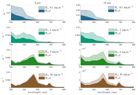
Figure 1.
Relative contribution of phytoplankton to total (with , and = 0.005 m) for increasing biomass with = 2 and 12 m. These populations are idealised examples and not intended to represent any observed relationship between Chl a concentration and .
For each , it is evident that the phytoplankton percentage contribution to the bulk increases with biomass. However, it can be seen that there is a dependency on which, when considered in the context of transitioning assemblages, is not straightforward. This observation indicates a requirement to go beyond the Case 1/Case 2 water type distinction for PFT signal analysis and applications: the differential in phytoplankton scatter as varies in both water types must be considered as well as variable in Case 2. When it comes to retrieving information about the phytoplankton IOPs, their proportional contribution to the bulk water-leaving signal (or the total IOPs) should be considered. Figure 2 demonstrates the proportional IOP contributions for the 0.1, 1 and 10 mg/m cases.
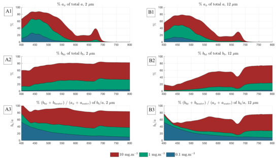
Figure 2.
Example proportional phytoplankton to total Inherent Optical Property (IOP) contributions for Case 1 waters, for idealised eukaryote assemblages of 2 and 12 m.
3.2. Case Study 1: Separating the Effects of Biomass from the Effects of Change
Figure 3 presents two distinct events which illustrate the interdependency of the size and biomass signals. Modelled are shown for selected adjacent stations (20 to 21 is marked A; 12 to 13 is marked B) where a nominal threshold of change detectable by satellite is reached in the blue and green spectral regions, in other words, where a change in would be evident on a satellite image. Given the ambiguity in the causality of the phytoplankton signal, assessing the magnitude of changes to the water-leaving signal as the in-water constituents vary will give an indication of whether there may be enough radiometric signal at TOA to even detect the change. A threshold in situ measurement resolution of 1 × 10 sr [80] is taken as an indication of sensitivity to detecting change in by direct measurement. Given an average estimated uncertainty in satellite of ± 0.6 × 10 sr across the spectrum [81], here a conservative 1 × 10 sr is used to indicate a potentially detectable change in water-leaving signal from satellite. These thresholds are not definitive and are used purely for the purpose of contextualising the discussion. Both examples in Figure 3 display large changes in , but these are causally distinct: (A) represents a large change in Chl a concentration and in , while (B) represents a large change in Chl a concentration but a negligible change in .

Figure 3.
Modelled for stations 20, 21, 12 and 13 of SOSCEX III. The modelled bulk are calculated using Equivalent Algal Populations (EAP) generalised Chl a-carotenoid refractive indices and measured Chl a concentrations for the phytoplankton component, and include estimated and contributions appropriate for this region [75,76]. Stations 20 to 21 (A) represent a large change in both Chl a concentration and in . Stations 12 to 13 (B) represent a large change in Chl a concentration only. The centre panel shows the measured for the cruise track (starting at the ice shelf on the bottom right and continuing in an anticlockwise direction.) The effective diameter image is courtesy of SANAE 55 Report [74].
Station 20 to 21 therefore represents a significant phytoplankton community shift, as large changes in both (from 6 to 16 m) and Chl a concentration (from 1 to 11 /m) were recorded. To isolate this change in phytoplankton signal, the differences in for an assemblage with = 6 m and an assemblage with = 16 m are presented in Figure 4A for the measured range of Chl a concentration. Note that the large differences of about 2 × 10 sr in in the blue, observable in Figure 3A, only appears at very low biomass in Figure 4A as this difference in is almost entirely due to the difference in biomass and not a change in . The spectral location of the most promising size-related signal for PFT retrieval is evidently dependent on biomass, and, at low biomass, it is positioned near 435 nm, while, at higher biomass, it is around 570 nm. As this is the phytoplankton-only signal, the question remains to what extent this signal is expressed in the bulk , when the optical impact of the non-algal constituents is also considered.
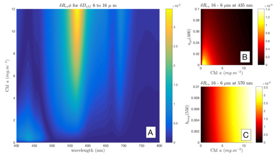
Figure 4.
Southern Ocean stations 20 to 21: is shown for of 6 to 16 m (A). The effect of at 435 nm is shown in (B), and at 570 nm in (C). The units of the colour bars are sr.
Working with the change in phytoplankton size signal identified at 435 nm (bottom left corner, Figure 4A), is added at increasing concentrations to simulate a range of bulk at 435 nm in Figure 4B, and is likewise added incrementally at 570 nm in Figure 4C. In these plots, horizontal gradients indicate sensitivity primarily to the constituent on the y axis, while vertical gradients indicate that the change in is driven by the biomass, and is not sensitive to variability on the y axis.
Figure 4B shows that the difference in bulk for the given is only detectable at the satellite threshold level (shown in yellow) at low biomass under very low conditions. As biomass increases, increasing absorption by phytoplankton as well as by additional , reduces the magnitude of the water-leaving signal and renders any information ambiguous. When additionally considering the brightening effect of in the blue (not quantified here), it can readily be perceived that the water-leaving signal is too complex at 435 nm to retrieve useful size information.
In Figure 4C, the relationship with at 570 nm is more straightforward. Change in due to is detectable in the bulk at the satellite threshold (in red) from about 2.5 mg/m upwards regardless of the contribution, at least for Case 1 type conditions. The magnitude of this signal is almost entirely biomass driven. (This is in line with the observation made by [13] that the MODIS wavebands at 531 and 551 nm are good indicators of backscatter anomalies because their magnitude is proportional to the addition or removal of particulate backscattering, and the longer wavelength band at 551 nm is less affected by variability in both and phytoplankton absorption [10].)
It should be appreciated, though, that in these figures is representing the change in due to size at a particular biomass (i.e., biomass is constant while assemblage characteristics vary), effectively removing the effects of simultaneous biomass changes. Figure 5 simulates a transition from 6 to 16 with biomass 1 to 11 mg/m, where the intermediate values of both and Chl a are simply linearly interpolated. The vertical lines highlight 435 and 570 nm which were identified in Figure 4A as being the spectral regions of greatest size-driven signal. In Figure 5, while biomass and size effects combine to form large changes in in the blue, it is the smaller signal around 570 nm that contains the most size-driven change as it is not affected by biomass to the same degree. Figure 4B,C show that the signal at 435 nm is sensitive to the effects of variable , while the phytoplankton signal at 570 nm remains robust against variability in the non-algal optical contributions.
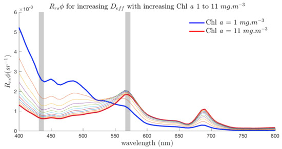
Figure 5.
A simulated transition from 6 to 16 with biomass 1 to 11 mg/m. Intermediate values of and Chl a are simply linearly interpolated. The lines highlight 435 nm and 570 nm, regions of maximum size signal, which are (at 435 nm) and are not (at 570 nm) sensitive to the effects of additional optical constituents.
By contrast, stations 12 to 13 exhibit a large change in —seen first in Figure 4B; shown again in Figure 6A—with an increase in Chl a from 0.9 to 7.1 mg/m but only a very small change in from 7 to 8 m. This is likely, given the location in the lee of the South Sandwich Islands, to reflect a diatom bloom associated with island wake effects, due to fertilisation by terrestrial iron [82]. Tracing the signal due to this change in across all Chl a concentrations in this range in Figure 6B shows that there is a size related signal between 550 and 600 nm, but it is of an order of magnitude less than in the previous example, and so does not show potential for detection by satellite radiometry. This is illustrated further in the lower panel (C), showing the location of this signal but also that it is almost all attributable to biomass—as shown by the representing 7 at 7.1 mg/m i.e., what the higher biomass would look like without the increase in effective diameter as the assemblage changes. It can be seen quite clearly from these spectra that a difference in the blue due only to this , with any variability , would not be detectable by any means.
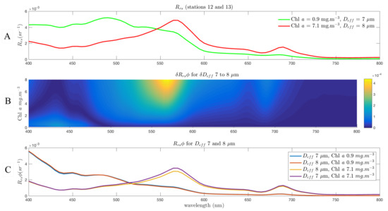
Figure 6.
Modelled for Stations 12 and 13 (A), with EAP eukaryote phytoplankton IOPs, and and components estimated guided by observations in [75,76], respectively; (B) shows for this large change in Chl a concentration (1 to 7 mg/m) but a small of 7–8 m. The unit of the colour bar is sr. Note that the results are one order of magnitude less than in the previous example; (C) shows the negligible effect on of a change in from 7 to 8 m at the measured Chl a concentrations.
It should be noted that the spectral locations of maximum features are a direct consequence of the spectral nature of the IOPs used in the modelling, and that both of these examples use the same Chl a-carotenoid refractive indices to generate the phytoplankton IOPs. In other words, as phytoplankton IOPs are adjusted to represent pigment differences, the spectral character of the assemblage change will vary. A slight migration in the exact location of the maximum available signal is observable with different ranges of , although within the Chl a-carotenoid group it remains between 550 and 600 nm for any difference in between 1 and 40 m. (This is discussed in more detail later with respect to Figure 9, and an additional figure is shown in Appendix.)
3.3. Case Study 2: Addressing Pigment Variability
Both the phycoerythrin-containing and peridinin-containing assemblages are modelled here, Figure 7 and Figure 8) with of 12 m, so the simulated optical changes as the assemblage changes from M. rubra-dominated to dinoflagellate-dominated are all due to differences in pigmentation, for any given Chl a concentration. From the log-scale it is evident that the pigment-related differences in become larger as biomass increases. In the very high biomass blooms (≥30 mg·m) typical of the Benguela system, it is known that M. Rubrum—containing assemblages are identifiable from MERIS satellite imagery [83] due to the effects of the diagnostic phycoerythrin peak (at 565 nm) appearing in the 560:520 nm band ratio.
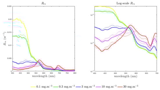
Figure 7.
Benguela-like pigment-based experiment: Modelled shown for Chl a-carotenoid pigmented assemblages (solid lines) and phycoerythrin containing assemblages (dotted lines) for identical Chl a concentrations, at 0.1, 0.3, 3, 10 and 30 mg·m. There is no change in , both are 12 m. The non-algal optical constituents are modelled with , and = 0.005 m.
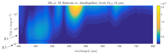
Figure 8.
shown for a change from a high biomass Myrionecta rubra-dominated assemblage, to a high biomass peridinin (carotenoid)-containing dinoflagellate-dominated assemblage. There is no change in .
An analogous study of the sensitivity of the maximum signal to non-algal constituents is made at 570 nm for the pigment-driven feature appearing at high biomass (10 mg·m, Figure 9). The sensitivity of pigment-driven differences to non-algal effects is in contrast to the Southern Ocean size example in that it is largely driven by variability in . As biomass increases past 10 mg·m, the magnitude of the grows as increases, showing no impact at all of biomass past 20 mg·m. What this means is that while significant biomass is required to detect pigment changes, past a certain upper biomass limit, the magnitude of the pigment differential signal grows proportionally as is augmented by non-algal scatter.
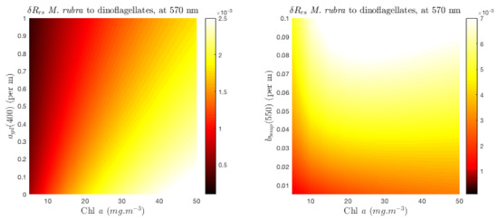
Figure 9.
sensitivity to and at 570 nm, for a high biomass Myrionecta rubra-dominated assemblage, to a high biomass peridinin (carotenoid)-containing dinoflagellate-dominated assemblage.
Absorption-based pigment differences are therefore sensitive to scattering variability unless the biomass is very high, and this is particularly relevant in spectral regions affected by scattering variability due to changes in (Figure 4). Noting the log-scale Chl a axis of Figure 9, it can be observed that while the respective magnitudes of the pigment-driven ( = 12 m, Figure 9) and size-driven ( from 6 to 16 m, Figure 4) signals are comparable at the point that pigment differences appear (i.e., 10 mg·m), the size-driven feature is more sensitive at lower biomass—detectable at around 2 mg·m for the given change in . This sensitivity will be affected by the size range in question and also by pigment concentrations, but it can be inferred that, generally, where size changes of this range (or larger) take place together with pigment changes, it is the size change that drives the variability in the water-leaving signal, and changes in the reflectance due to a substantial change in are observable at lower biomass than those due to pigment changes.
This applies equally to accessory pigments other than phycoerythrin absorbing in spectral regions affected by phytoplankton scatter and/or by variability in non-algal scatter. This speaks to the importance of both the magnitude of the change in and the proportional contribution of to the total when evaluating the potential for accessing these signals from (see Figure 2).
This result also implies that there are cases where the signal is augmented by pigment changes, for example when moving from small fucoxanthin- or peridinin-dominated cells to large phycoerythrin-dominated cells, as the optical effect of reduction in backscatter around 560–570 nm by large cells will be enhanced by additional pigment absorption in the signal. However, there remains a complex optical relationship with biomass, and this effect needs to be properly accounted for in order to accurately detect the augmented signal.
The EAP approach to pigments does not address the extent to which fine spectral resolution accessory pigment absorption features persist in , nor their retrieval from hyperspectral radiometry. The intention with the EAP model is to demonstrate the dependence on biomass to retrieve absorption features, and the inherent signal ambiguity as the contrasting optical effects of and interact to form the phytoplankton signal within the . It is worth noting that hyperspectral radiometry will not overcome the inherent signal-related constraints identified in this study.
3.4. Radiometric Sensitivity of EAP Size-Based PFT Detection—Magnitude of
Having established that at low biomass the PFT signal in the blue is easily overwhelmed by the effects of and , and that pigment effects are generally secondary to those of , the PFT signal due to phytoplankton scattering in the 500 to 600 nm region can be evaluated for sensitivity in terms of changes in and biomass. To this end, the EAP model is again coupled with Hydrolight to simulate expected variability in due to changes in with the aim of evaluating the sensitivity of the model.
Figure 10A demonstrates how the combined effects of biomass and interact to form the maximum available signal at low biomass and small size ranges. The figure shows that this maximum lies between 520 and 570 nm—the exact wavelength varies with both size difference and biomass. The shifting position of maximum is shown in Figure 10B. Increasing biomass improves the ability to trace the size-related effects, and a change from 2 m up to at least 8 m is not detectable at the threshold in oceanic conditions with Chl a< 1 mg/m.
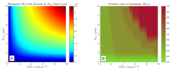
Figure 10.
Maximum for from a starting assemblage with 2 m, as Chl a varies (A). Note that the occurs at different wavelengths from 500 to 600 nm (B), and this shows the maximum signal, so there is no exact wavelength information in (A). Using a difference of 1 × 10 sr as a threshold for detection by satellite, it can be seen that, while the maximum size change here (2 to 8 m) is not detectable with Chl a < 1 mg/m, by 10 mg/m, even a small change in results in a detectable change in .
Using 1 × 10 sr as a threshold for detection by satellite, it can be seen that an ecologically significant shift in from 2 or 3 to 6 m, such as at the onset of an oceanic bloom, looks potentially detectable from about 2 mg/m. By 10 mg/m, even a small change in results in a detectable change in , but, as biomass falls below this, the change in must be increasingly large to be detected. This is consistent with inversion studies of EAP sensitivity [37]. Note that this experiment addresses only the phytoplankton-related signal, and that when attempting to identify these signals in the bulk , it is necessary to consider the sensitivity of the phytoplankton signal to the optical effects of the non-algal constituents. These results can be considered to show the minimum threshold for potential detection i.e., the signal is further ambiguated by non-algal optics in a real-world context.
The spectrally shifting nature of the signal for oceanic PFT applications provides a strong case for hyperspectral sensors in the 520 to 570 nm wavelength region. The extent to which the signal persists in fixed waveband ratios is investigated in the next section on shape sensitivity.
3.5. Spectral Shape Sensitivity of EAP Size-Based PFT Detection
To further test the sensitivity of the EAP model and the causal IOP variability in terms of identifiable changes in spectral shape from a multi-spectral perspective, ratios for 440:560 nm (blue:green), 560:665 nm (green:red) and 665:710 nm (red:NIR) wavelengths were calculated for a range of and biomass.
These are shown in Figure 11, representing corresponding changes in the and in the phytoplankton backscattering, for these wavelength pairs. The B:G ratio shows a strong biomass dependency and a small sensitivity to size at large sizes, for 0.5 ≤ Chl a≤ 4.5 mg/m. The R:NIR ratio shows some sensitivity to larger sizes from about 3 mg/m, but this decreases as biomass increases. The G:R ratio shows a significant size-related feature for small sizes (≤ 6 m) from biomass of about 2 mg/m upwards (encircled in Figure 10). This is where a peak in the corresponding b ratio appears, suggesting that the large change in magnitude of the Chl a-specific backscatter between small (Figure 12) is directly responsible for the sensitivity in the G:R ratio seen in Figure 11.
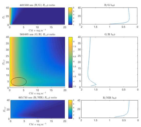
Figure 11.
ratios for blue:green, green:red and red:NIR (Near Infra-Red) wavelengths as shown, for Chl a concentrations of 0.1 to 20 mg/m and 1 to 40 m. The B/G ratio shows a strong biomass dependency and a small sensitivity to size at large sizes, for 0.5 ≤ Chl a≤ 4.5 mg/m. The b ratios all display a strong size signal at 2–4 m, and the G/R ratio shows a corresponding size-related feature.
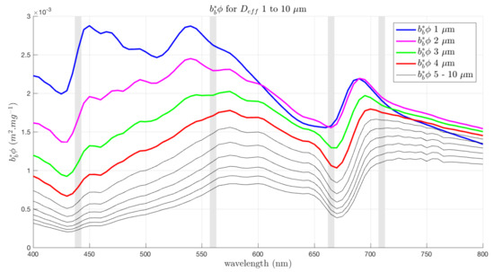
Figure 12.
shown for 1 to 10 m. The largest differences in backscatter across the spectrum occur between 1 and 4 m, with the exception of the overlapping of in the red and NIR.
This is an important finding. There is a marked size dependency in all of the ratios, with the greatest rate of change somewhere between 2 and 8 m, but it is only in the case of the G:R ratio that the magnitude of the backscatter is sufficient for this signal to be identifiable in the . Given that the radiometric signal in the blue is greatly reduced by large phytoplankton absorption and , and the red and NIR wavelengths are similarly affected by the absorption of water, it can be concluded that the main driver of the useable PFT signal in the green and red is phytoplankton backscatter.
Figure 13 shows the rapid increase in the proportional contribution of phytoplankton to total backscatter at 560 and 665 nm. It is known that, for typical diatom/dinoflagellate assemblages, the 560 nm region is more influenced by backscatter than by absorption. The fact that the magnitude of the total backscatter is much lower at 665 than at 560 nm, together with the strong absorption by water in this region, result in a small useable signal. A contribution of approximately 40% of phytoplankton to total at 560 nm corresponds with the limits of detectable (see Figure 2), indicating that this is the proportion at which phytoplankton backscatter starts driving the total water-leaving signal around 560 nm. Consequently, this is the minimum contribution for which some information may be known. For an oceanic bloom example from 2–6 m, this threshold contribution is reached at about 2 mg/m, while to detect an example of 10 to 20 m in a eukaryotic succession, extremely high biomass is required. The mid-range biomass sensitivity demonstrated here presents opportunities for identifying higher resolution size classes than the 2 to 20 m and >20 m categories currently frequently employed [6,8,10,84]. The ability to achieve better resolution within the 2–20 m size class is particularly desirable for marine ecosystem modelling [6].
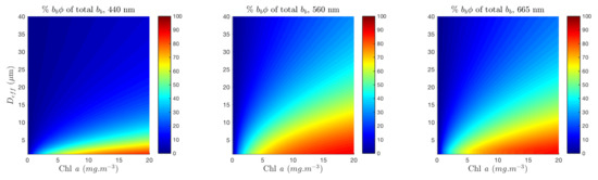
Figure 13.
Percentage contribution of phytoplankton to total backscatter (including water, and with nominal (550) = 0.005), shown for 1 to 40 m and Chl a from 0.1 to 20 mg/m, at 440, 560 and 665 nm.
3.6. Considering Uncertainties
Particularly when considering retrievals from satellite, it is important and necessary to contextualise the magnitude of the PFT signal with respect to uncertainties on the satellite radiometry. A brief study on model and associated radiometric uncertainty is available in Appendix D. An important observation is that, while the 500 to 600 nm region of the promising PFT signal may be mostly insensitive to the effects of non-algal constituents, it is also where variability in due to the different approaches to phytoplankton phase functions is important, emphasising the critical role of phytoplankton scatter in this signal.
4. Conclusions
The distinct causal optical effects of variations in phytoplankton biomass, mean assemblage size, pigment-related spectral variability and non-algal constituents are not easily identified, with substantial interdependency and spectral ambiguity. Consistent with previous studies [37,39], it can be seen here that ambiguity is critical in attempting to resolve the phytoplankton community structure signals.
The case studies illustrate how most of the signal that is due to phytoplankton is driven by biomass, an expected result. This concept underpins, after all, the primary missions of most ocean colour sensors: resolving variability in phytoplankton biomass. The study shows that quantitative consideration of the constraints of biomass and the phytoplankton contribution to the total IOP budget is required when addressing the PFT question.
The key findings include the assertions that most of the absorption driven phytoplankton signal in in the blue is too ambiguous to use, and that the most useful PFT signal is caused by spectral backscatter. Furthermore, the ability to assess the PFT signal against non-algal optical contributions is largely driven by biomass and the IOP budget.
Overall, spectral scattering properties of natural waters are not well characterised [85,86], and phytoplankton spectral backscattering characteristics are underexploited in terms of their impact on the water-leaving signal. The importance of better representing the angular and spectrally variable nature of phytoplankton scattering has been established [35], and it is clear that phytoplankton backscatter is at the heart of the PFT question.
The size-related PFT signal is driven by phytoplankton scattering, and spectral regions where scattering is at its most sensitive to show the most potential for PFT detection from the total water-leaving signal. There is most sensitivity to size-related changes in in the 1–6 m size range. Phytoplankton size-related features, most likely driven by phytoplankton absorption variablity, appear in around 430 nm at low biomass, and scattering-driven size-related features in the 520 to 570 nm spectral region at elevated biomass. The water-leaving signal in the blue spectral region is highly complex and ambiguous, being the result of varied and contrasting effects of absorbing and scattering characteristics of both algal and non-algal in-water constituents. Consequently, the size-related signal appearing in low biomass waters (<1 mg/m) may be useful only when and are exactly known. Accessory pigment absorption features that persist in in low biomass suffer from the same vulnerability to uncertainty in the non-algal constituents. Satellite measurement uncertainty and retrievals may in future be improved (e.g., with the use of radiometry in the UV), but, given current uncertainties, achieving sufficiently accurate satellite estimates of the non-algal optical components is unlikely for this purpose.
This finding exposes a vulnerability in historical approaches to phytoplankton identification and quantification based on the features of phytoplankton absorption characteristics in the blue. Satellite PFT methods using this approach all suffer from this shortcoming where assemblage-related variability is secondary to biomass effects, and where phytoplankton relationships with and are not precisely known. These approaches additionally rely on implicit relationships between Chl a and which may not always hold. This work shows that, at low biomass (< 1 mg·m), where is absorption-dominated, it is unlikely that there is sufficient size- or pigment-driven PFT signal to be retrieved from satellite radiometry without making these assumptions. (Phytoplankton whose prominent absorption features are at longer wavelengths, such as phycocyanin-containing cyanobacteria, present a different case). Isolating variability in as and biomass vary shows that an example oceanic bloom from 2 to 6 m is only detectable at the satellite measurement threshold of 1 × 10 sr when the biomass reaches about 2 mg/m (Figure 10A).
Consequently, it is the size-related backscatter-driven signal in the 500 to 570 nm region, appearing at substantial biomass, that is the most useful for PFT identification from satellite radiometry as it is sufficiently insensitive to reasonable variability in both and (when composed of small particles) (Figure 4). Variability in scatter due to non-algal particulate in the same size range as phytoplankton will likely ambiguate the distinctive spectral scatter of PFT changes, and this has not yet been tested. The location of the maximum size feature shifts between 520 and 570 nm (Figure 10B), suggesting strongly that hyperspectral data in this region would add greater capability here. Further analysis is needed to quantify the potential advantages of hyper- over multi-spectral data with respect to this shifting maximum signal, and also with respect to the reduced SNR implicit in narrow waveband measurements.
Understanding the proportional phytoplankton contribution to the total IOP budget and the resulting water-leaving signal is central to the determination of sufficient phytoplankton-driven signal containing PFT information. The proportional ’net’ contribution of phytoplankton i.e., as a percentage of total , has been identified as the driver of PFT sensitivity in the . Given the detectable differences in as size and biomass change, a proportional phytoplankton contribution of approximately 40% to the total appears to a reasonable minimum threshold in terms of yielding a detectable optical change. The proportional contribution always varies with the non-algal optical constituents and .
Despite the many sources of model uncertainty and the requirement for model validation in specific regions, these results indicate the necessity of approaching PFTs from a strongly biophysical perspective. There is a great need for better characterisation of phytoplankton community structure and improved handling of the complex spectral and angular nature of phytoplankton scattering.
The EAP model code in Matlab R2018a (The Mathworks Inc., Natick, Mass, United States) or in Python 3.7, as well as the Fortran routine for Hydrolight allowing the choice of discretised EAP phase function based on wavelength rather than backscatter fraction (see Appendix D: Uncertainties), are freely available to the community. Please contact the corresponding author.
Supplementary Materials
The following are available online at http://www.mdpi.com/2076-3417/8/12/2681/s1, Visualisation Tool: Interactive visualisation of spectral with assemblage shown for 2–20 m, with user-controlled Chl a concentration, and .
Author Contributions
Conceptualization, L.R.L. and S.B.; Formal analysis, L.R.L.; Investigation, L.R.L.; Project administration, S.B.; Software, L.R.L.; Supervision, S.B.; Writing—original draft, L.R.L.; Writing—review & editing, S.B.
Funding
Funding that was awarded to Lisl Robertson Lain from the Centre for Scientific and Industrial Research (CSIR) and the University of Cape Town (UCT) PhD Scholarship Programme is gratefully acknowledged, as is funding from the CSIR/DST SWEOS Strategic Research Programme.
Acknowledgments
Thanks to Curtis Mobley for assistance with Hydrolight and the examiners of Lisl Robertson Lain’s PhD thesis for their valuable comments. Input from two anonymous reviewers of this manuscript, as well as from Dariusz Stramski, was gratefully received.
Conflicts of Interest
The authors declare no conflict of interest.
Appendix A. Phytoplankton Assemblage Variability in the EAP Model
The successful validation of the model in very high biomass Benguela conditions [65] gives confidence in the representation of the phytoplankton component of the water-leaving signal, as it is known that, in these cases, the is overwhelmingly dominated by phytoplankton. It is concluded in Lain et al. [65] that it is the EAP’s detailed handling of phytoplankton spectral backscatter that sets it apart from other IOP models. The core mathematics of the model are fully described in Bernard et al. [27]. A detailed study of EAP phytoplankton angular scattering and phase functions is available in Lain et al. [35].
Appendix A.1. Justification for Using Measurement-Derived Refractive Indices across Wide Size Ranges
The main light-harvesting pigments in typical diatom and dinoflagellate assemblages (fucoxanthin and peridinin, respectively)—while chemotaxonomically distinct—display the typical broad, featureless absorption spectra characteristic of carotenoids, with peaks centered around 500 nm [87] and vary well within the natural variability of phytoplankton absorption (Figure A1). They consequently have similar refractive indices [27] and so these types were combined into a generalised set of diatom/dinoflagellate IOPs, as no significant difference was found between the dinoflagellate and diatom groups in terms of their optics that could not be attributed to the respective particle sizes (see also [38,88]). This group of IOPs should correctly be referred to as Chl a-carotenoid IOPs.

Figure A1.
Pigment absorption spectra from Bricaud et al. [87], reprinted with permission from the American Geophysical Union. The broad featureless absorption spectra of fucoxanthin and peridinin peaking at around 500 nm are shown by the thin and thick brown lines, respectively.
While the measurements and refractive index derivations [89] were performed for cells of approximately 12 to 20 m, it should be made clear that the imaginary refractive index characterises the absorption of the intracellular material and has absolutely no dependency on cell size. It can be inferred therefore that these refractive indices can be used to represent a range of phytoplankton sizes displaying dominant Chl a and carotenoid pigments. Southern Ocean nanophytoplankton comprise mainly diatoms and dinoflagellates, but also chlorophytes and haptophytes in smaller proportions [90,91]. The latter two phytoplankton groups are generally dominated by Chl a and the fucoxanthin pigment derivatives 19’-hex-fucoxanthin and 19’-but-fucoxanthin [91], which display somewhat elevated absorption peaks located at slightly shorter wavelengths with respect to fucoxanthin [87,92]. The optical influence of these derivative pigments is assumed to be negligible in the context of the case studies for two reasons. Firstly, in the nanophytoplankton group as a whole, the fucoxanthin-derived pigments occur in far lesser concentrations than that of fucoxanthin itself [91], which is represented by the refractive indices. This is reinforced by the derivation of a nanophytoplankton group of refractive indices in non-bloom conditions ( = 2 m), whose impact on the IOPs of small cells was not sufficiently different from the diatom-dinoflagellate group to warrant its routine use for small cells. Secondly, these pigments act to increase phytoplankton absorption around the 450 nm spectral region, identified the spectral region as very vulnerable to small variability in , and to large satellite measurement uncertainty, so the conclusions regarding the spectral regions containing the most useful signatures for PFT detection still hold.
EAP sensitivity testing has indicated that increasing the intracellular Chl a density may be appropriate for small cells, but this is not explored here.
Appendix A.2. EAP Phytoplankton IOPss
Phytoplankton-specific IOPs are presented in Figure A5 and Figure A6 for generalised Chl a-carotenoid assemblages and for phycoerythrin-containing assemblages, respectively.

Figure A2.
EAP Eukaryote Chl a-carotenoid-dominated IOPs for a range of assemblage .

Figure A3.
EAP Phycoerythrin-containing IOPs (based on Myrionecta Rubra), used for cryptophyte-dominated assemblages in the Benguela, and Synechococcus sp. in the Southern Ocean.
Appendix A.3. EAP agd(λ) Parameterisation
A simple exponential combined gelbstoff and detrital absorption term [93,94] is used as a representative of commonly occurring conditions in the Benguela:
The exponential slope factor S is given a constant value of 0.012 [95]. This value, derived for the Benguela system, is not adjusted for the term used in the Southern Ocean Case Studies. This is acknowledged as a source of uncertainty, but supporting literature suggests that values in the range 0.0140 ± 0.0032 nm cater adequately for a variety of water types [93].
An observed relationship of
from measurements in the Benguela is used to scale the gelbstof/detrital exponential term, and onwards is assumed to be zero. This parameterisation was derived for high biomass environments. At very low biomass (< 1 mg/m), the term becomes negative, and so, for the Southern Ocean case studies, this parameterisation was amended to
following Alvain et al. [21], noting that the referenced parameterisation is for 440 nm and not 400, but also that the term is used as an approximate measure of total signal sensitivity, and so, in this sense, an absolutely accurate term is not a requirement.
Appendix A.4. EAP bbnap(λ) Parameterisation
Non-algal backscattering is modelled after Roesler and Perry [96] who describe a small particle backscattering term represented by a power law relationship (their , referred to as in the EAP model). It has a constant spectral shape dependent only on wavelength, but variable in magnitude.
This is then adjusted to a selected value of , as detailed in the text.
Small particle (non-algal) scatter is approximated as 50 times the in the Benguela examples and as 100 times the in the Southern Ocean examples. This yields a non-algal particulate backscattering probability () of 0.02 (2%) and 0.01 (1%), respectively. This is assumed to be reasonable given that it has been shown that the total particulate backscattering probability varies in the range 1.2 to 3.2 % in coastal waters dominated by non-algal particles (i.e., Case 2) [97], and that generally accepted values for in Case 1 waters is around 1% [98].
Keeping the non-phytoplankton backscattering constant with Chl a results in a dependent but nonlinear relationship, resulting in an overall that decreases as Chl a increases (Figure A4), noting the spectral variability of small phytoplankton at elevated biomass.

Figure A4.
Bulk backscatter ratio shown for 2 and 12 m, with nominal (550) = 0.01 m and as 50 times the , as for a coastal environment, shown for Chl a of 0.5, 1.0 and 2.0 mg/m. The elevated backscatter ratio of coastal environments with respect to the Southern Ocean (where is modelled as 100 times the ) is attributed to the contribution of terrestrial mineral particles with a high refractive index [66,99].
Appendix B. Measurements and Modelling Parameters
Appendix B.1. Chl a
Chl a measurements are made using a Turner 10-AU Fluorometer (Turner Designs, San Jose, CA, USA), following Holm-Hansen et al. [100].
Appendix B.2. Model Parameters Used for Hydrolight-Ecolights
For most of the experiments, Ecolight’s 2-component IOP model was used to generate . The “clearest natural water” IOPs were selected for Component 1 (water). IOPs for component 2 (everything else) were precomputed in Matlab from the EAP phytoplankton IOPs and additional and contributions as required.
Fluorescence quantum efficiency was approximated by Chl a concentration:
<10 mg/m3 = 1%
10–50 mg/m3 = 0.6%
50–100 mg/m3 = 0.2%
>100 mg/m3 = 0.1%.
These values are based on MODIS climatologies [101], and measurements [102] to characterise the reduction in as eutrophication increases.
A constant set of generalised atmospheric conditions was selected for all experiments. An annual average for solar irradiance and a solar zenith of 30 was used in lieu of time and location.
Appendix C. Position of Maximum δRrsϕ
Further to Figure 9B in the main text, Figure A5 shows the position of maximum for assemblage changes from 8 m and 14 m, respectively, for Chl a concentrations between 10 and 20 mg/m. It can be seen that, at these high biomass concentrations, there is no spectral migration of the maximum with biomass, and that once the maximum signal reaches 570 nm, its location does not change with increasing for biomass up to 20 mg/m. This has been tested up to 40 m (not shown).

Figure A5.
Spectral position of maximum for assemblage changes from 8 m and 14 m, respectively.
Appendix D. Uncertaintiess
Uncertainties in satellite radiometry are given in the main text, and model error in terms of uncertainty/variability in the phase function is described fully in [35]. There are many additional sources of uncertainty in the model (non-sphericity of phytoplankton, approximations in size distribution, Chlorophyll a density, to name a few), and further work is needed to quantify them appropriately. For demonstrative purposes here, given that any retrieval of size properties would be performed with the model itself, the model uncertainty is constrained to just that of the phase function variability, as this has a size implication in itself, as shown in [35].
In Figure A6, the model uncertainty is shown for against a background of total with nominal additional and , together with the satellite measurement uncertainty. Despite the small model uncertainty on the phytoplanton signal in the blue, the huge impact of additional and the large satellite radiometric uncertainty clearly show the large degree of ambiguity and potential error in the retrieval of the phytoplankton component, even if the is exactly known. Satellite-derived (and CDOM) products have large uncertainties: of less than 0.25 for three different algorithms against in situ data [16]—noting that dependence on the atmospheric correction means that a significant level of error is propagated through the algorithms from this source, particularly in the blue.

Figure A6.
Total with satellite measurement uncertainties in the blue and red bands from [16] and linearly interpolated between them. An indication of model uncertainty on the is calculated by the spectral differences resulting from the use of a combined -specific Fournier Forand phase function independent of wavelength, vs. wavelength- and -dependent EAP phase functions.
The most significant spectral regions of Figure A6 in the context of this study are those where the uncertainty on overlap with the bulk satellite measurement uncertainty in each example. These are the spectral regions where the phytoplankton-specific signal dominates the bulk signal to the point that they are arguably indistinguishable, so these regions are particularly promising in terms of PFT detection from the bulk . It is also encouraging to note that the regions of maximum previously identified fall within these regions, meaning that particularly close to 570 nm, the bulk signal not only closely reflects the causal phytoplankton signal but is also not very sensitive to reasonable variability in and . However, it is an important consideration that these are also regions of large uncertainty in the size signal, and that, as increases, the expression of reduced phytoplankton scatter becomes more vulnerable to variable .
At low biomass, the phytoplankton signal falls well outside of the bulk measurement uncertainty, but the question of whether phytoplankton IOPs could be retrieved from the bulk depends on the resulting proportional contribution to the total. With reduced , even small variability in the non-algal contribution to results in signal ambiguity. In this case, the additional and contributions need to be exactly known, in order to be able to retrieve any PFT information.
It can also be observed in Figure A6 that the magnitude of model uncertainty is less, and the proportional contribution of phytoplankton to the bulk IOPs is greater, at wavelengths slightly shorter than those of the maximum in the case studies. Thus, the spectral location of the largest observable signal may not necessarily be the most revealing of PFT discrimination in terms of the associated uncertainties. A sophisticated uncertainty model would be necessary to calculate the respective advantages of reduced contribution uncertainties on a smaller signal vs. slightly larger uncertainties on a larger workable signal. It is also worth considering that, even where the bulk and signals are distinct, there are spectral regions where they are parallel i.e., maintain the same shape. It can be concluded that the phytoplankton contribution determines the spectral shape in these regions—although the uncertainty associated with a smooth curve is also not quantified here. This information could potentially be exploited to investigate PFT signal from the bulk .
Further work on incorporating EAP phase functions into Hydrolight has enabled the presented here to include the fluorescence term, and this is also a spectral region of a large proportional phytoplankton contribution together with small model uncertainty as calculated by the difference in approach to scattering phase functions. This region (around 685 nm) appears in the maximum plots from the case studies, but has not been discussed as confidence in modelling this spectral region accurately needs to be improved with respect to natural variability in a fluorescence quantum yield and phytoplankton response to the light environment. However, it is known that this region holds further useful information on phytoplankton health [103] as well as size.
Overall, the uncertainties in both measured and modelled quantities should be considered in terms of the proportional contribution by phytoplankton. The highest proportional phytoplankton contribution to the bulk optics, and therefore the most promising signal for PFTs, occurs where elevated scatter due to biomass is complemented by the elevated scatter of small phytoplankton cells. Approaches to modelling the phase functions result in an inherent ambiguity of about 4 m at very high biomass, but this drops with biomass and as increases.
References
- Field, C.B.; Behrenfeld, M.J.; Randerson, J.T. Primary production of the biosphere: Integrating terrestrial and oceanic components. Science 1998, 281, 237–240. [Google Scholar] [CrossRef] [PubMed]
- McClain, C.R. A decade of satellite ocean color observations. Annu. Rev. Mar. Sci. 2009, 1, 19–42. [Google Scholar] [CrossRef] [PubMed]
- Swart, S.; Chang, N.; Fauchereau, N.; Joubert, W.; Lucas, M.; Mtshali, T.; Roychoudhury, A.; Tagliabue, A.; Thomalla, S.; Waldron, H.; et al. Southern Ocean Seasonal Cycle Experiment 2012: Seasonal scale climate and carbon cycle links. S. Afr. J. Sci. 2012, 108, 11–13. [Google Scholar] [CrossRef]
- Thomalla, S.; Fauchereau, N.; Swart, S.; Monteiro, P. Regional scale characteristics of the seasonal cycle of chlorophyll in the Southern Ocean. Biogeosciences 2011, 8, 2849. [Google Scholar] [CrossRef]
- Ryan-Keogh, T.J.; Thomalla, S.J.; Mtshali, T.N.; Little, H. Modelled estimates of spatial variability of iron stress in the Atlantic sector of the Southern Ocean. Biogeosciences 2017, 14, 3883–3897. [Google Scholar] [CrossRef]
- Brewin, R.J.W.; Ciavatta, S.; Sathyendranath, S.; Jackson, T.; Tilstone, G.; Curran, K.; Airs, R.L.; Cummings, D.; Brotas, V.; Organelli, E.; et al. Uncertainty in Ocean-Color Estimates of Chlorophyll for Phytoplankton Groups. Front. Mar. Sci. 2017, 4, 104. [Google Scholar] [CrossRef]
- Antoine, D.; d’Ortenzio, F.; Hooker, S.B.; Bécu, G.; Gentili, B.; Tailliez, D.; Scott, A.J. Assessment of uncertainty in the ocean reflectance determined by three satellite ocean color sensors (MERIS, SeaWiFS and MODIS-A) at an offshore site in the Mediterranean Sea (BOUSSOLE project). J. Geophys. Res. Oceans 2008, 113, 2156–2202. [Google Scholar] [CrossRef]
- Sathyendranath, S.; Watts, L.; Devred, E.; Platt, T.; Caverhill, C.; Maass, H. Discrimination of diatoms from other phytoplankton using ocean-colour data. Mar. Ecol. Prog. Ser. 2004, 272, 59–68. [Google Scholar] [CrossRef]
- Alvain, S.; Loisel, H.; Dessailly, D. Theoretical analysis of ocean color radiances anomalies and implications for phytoplankton groups detection in Case 1 waters. Opt. Express 2012, 20, 1070–1083. [Google Scholar] [CrossRef]
- Kostadinov, T.; Siegel, D.; Maritorena, S. Retrieval of the particle size distribution from satellite ocean color observations. J. Geophys. Res. Oceans 2009, 114. [Google Scholar] [CrossRef]
- Kostadinov, T.S. Carbon-based phytoplankton size classes retrieved via ocean color estimates of the particle size distribution. Ocean Sci. 2016, 12, 561. [Google Scholar] [CrossRef]
- Anderson, T.R. Plankton functional type modelling: Running before we can walk? J. Plankton Res. 2005, 27, 1073–1081. [Google Scholar] [CrossRef]
- Brown, C.A.; Huot, Y.; Werdell, P.J.; Gentili, B.; Claustre, H. The origin and global distribution of second order variability in satellite ocean color and its potential applications to algorithm development. Remote Sens. Environ. 2008, 112, 4186–4203. [Google Scholar] [CrossRef]
- MÉlin, F.; Sclep, G.; Jackson, T.; Sathyendranath, S. Uncertainty estimates of remote sensing reflectance derived from comparison of ocean color satellite data sets. Remote Sens. Environ. 2016, 177, 107–124. [Google Scholar] [CrossRef]
- Lee, Z.P. Remote Sensing of Inherent Optical Properties: Fundamentals, Tests of Algorithms and Applications. Rep. Int. Ocean Colour Coord. Group 2006, 5, 1–122. [Google Scholar]
- Mélin, F.; Zibordi, G.; Berthon, J.F. Assessment of satellite ocean color products at a coastal site. Remote Sens. Environ. 2007, 110, 192–215. [Google Scholar] [CrossRef]
- Mouw, C.B.; Hardman-Mountford, N.J.; Alvain, S.; Bracher, A.; Brewin, R.J.W.; Bricaud, A.; Ciotti, A.M.; Devred, E.; Fujiwara, A.; Hirata, T.; et al. A Consumer’s Guide to Satellite Remote Sensing of Multiple Phytoplankton Groups in the Global Ocean. Front. Mar. Sci. 2017, 4, 41. [Google Scholar] [CrossRef]
- Hirata, T.; Hardman-Mountford, N.J.; Brewin, R.J.W.; Aiken, J.; Barlow, R.; Suzuki, K.; Isada, T.; Howell, E.; Hashioka, T.; Noguchi-Aita, M.; et al. Synoptic relationships between surface Chlorophyll-a and diagnostic pigments specific to phytoplankton functional types. Biogeosciences 2011, 8, 311–327. [Google Scholar] [CrossRef]
- Brewin, R.J.W.; Hardman-Mountford, N.J.; Lavender, S.J.; Raitsos, D.E.; Hirata, T.; Uitz, J.; Devred, E.; Bricaud, A.; Ciotti, A.; Gentili, B. An intercomparison of bio-optical techniques for detecting dominant phytoplankton size class from satellite remote sensing. Remote Sens. Environ. 2011, 115, 325–339. [Google Scholar] [CrossRef]
- Brewin, R.J.W.; Sathyendranath, S.; Hirata, T.; Lavender, S.J.; Barciela, R.M.; Hardman-Mountford, N.J. A three-component model of phytoplankton size class for the Atlantic Ocean. Ecol. Modell. 2010, 221, 1472–1483. [Google Scholar] [CrossRef]
- Alvain, S.; Moulin, C.; Dandonneau, Y.; Bréon, F.M. Remote sensing of phytoplankton groups in Case 1 waters from global SeaWiFS imagery. Deep Sea Res. Part I Oceanogr. Res. Pap. 2005, 52, 1989–2004. [Google Scholar] [CrossRef]
- Alvain, S.; Moulin, C.; Dandonneau, Y.; Loisel, H. Seasonal distribution and succession of dominant phytoplankton groups in the global ocean: A satellite view. Glob. Biogeochem. Cycles 2008, 22, 1–15. [Google Scholar] [CrossRef]
- Devred, E.; Sathyendranath, S.; Stuart, V.; Platt, T. A three component classification of phytoplankton absorption spectra: Application to ocean-color data. Remote Sens. Environ. 2011, 115, 2255–2266. [Google Scholar] [CrossRef]
- Ciotti, A.M.; Bricaud, A. Retrievals of a size parameter for phytoplankton and spectral light absorption by colored detrital matter from water-leaving radiances at SeaWiFS channels in a continental shelf region off Brazil. Limnol. Oceanogr. Methods 2006, 4, 237–253. [Google Scholar] [CrossRef]
- Bracher, A.; Vountas, M.; Dinter, T.; Burrows, J.; Röttgers, R.; Peeken, I. Quantitative observation of cyanobacteria and diatoms from space using PhytoDOAS on SCIAMACHY data. Biogeosciences 2009, 6, 751–764. [Google Scholar] [CrossRef]
- Kostadinov, T.S.; Siegel, D.A.; Maritorena, S. Global variability of phytoplankton functional types from space: assessment via the particle size distribution. Biogeosciences 2010, 7, 3239–3257. [Google Scholar] [CrossRef]
- Bernard, S.; Probyn, T.A.; Quirantes, A. Simulating the optical properties of phytoplankton cells using a two-layered spherical geometry. Biogeosci. Discuss. 2009, 6, 1497–1563. [Google Scholar] [CrossRef]
- Uitz, J.; Stramski, D.; Reynolds, R.A.; Dubranna, J. Assessing phytoplankton community composition from hyperspectral measurements of phytoplankton absorption coefficient and remote-sensing reflectance in open-ocean environments. Remote Sens. Environ. 2015, 171, 58–74. [Google Scholar] [CrossRef]
- Torrecilla, E.; Stramski, D.; Reynolds, R.A.; Millán-Núñez, E.; Piera, J. Cluster analysis of hyperspectral optical data for discriminating phytoplankton pigment assemblages in the open ocean. Remote Sens. Environ. 2011, 115, 2578–2593. [Google Scholar] [CrossRef]
- Xi, H.; Hieronymi, M.; Röttgers, R.; Krasemann, H.; Qiu, Z. Hyperspectral differentiation of phytoplankton taxonomic groups: A comparison between using remote sensing reflectance and absorption spectra. Remote Sens. 2015, 7, 14781–14805. [Google Scholar] [CrossRef]
- Sadeghi, A.; Dinter, T.; Vountas, M.; Taylor, B.; Altenburg-Soppa, M.; Bracher, A. Remote sensing of coccolithophore blooms in selected oceanic regions using the PhytoDOAS method applied to hyper-spectral satellite data. Biogeosciences 2012, 9, 2127–2143. [Google Scholar] [CrossRef]
- Stramski, D.; Bricaud, A.; Morel, A. Modeling the inherent optical properties of the ocean based on the detailed composition of the planktonic community. Appl. Opt. 2001, 40, 2929–2945. [Google Scholar] [CrossRef] [PubMed]
- Matsuoka, A.; Huot, Y.; Shimada, K.; Saitoh, S.I.; Babin, M. Bio-optical characteristics of the western Arctic Ocean: Implications for ocean color algorithms. Can. J. Remote Sens. 2007, 33, 503–518. [Google Scholar] [CrossRef]
- Bernard, S.; Shillington, F.A.; Probyn, T.A. The use of equivalent size distributions of natural phytoplankton assemblages for optical modeling. Opt. Express 2007, 15, 1995–2007. [Google Scholar] [CrossRef] [PubMed]
- Lain, L.R.; Bernard, S.; Matthews, M.W. Understanding the contribution of phytoplankton phase functions to uncertainties in the water colour signal. Opt. Express 2017, 25, A151–A165. [Google Scholar] [CrossRef] [PubMed]
- Morel, A. Consequences of a Synechococcus bloom upon the optical properties of oceanic (case 1) waters. Limnol. Oceanogr. 1997, 42, 1746–1754. [Google Scholar] [CrossRef]
- Evers-King, H.; Bernard, S.; Lain, L.R.; Probyn, T.A. Sensitivity in reflectance attributed to phytoplankton cell size: Forward and inverse modelling approaches. Opt. Express 2014, 22, 11536–11551. [Google Scholar] [CrossRef]
- Organelli, E.; Nuccio, C.; Lazzara, L.; Uitz, J.; Bricaud, A.; Massi, L. On the discrimination of multiple phytoplankton groups from light absorption spectra of assemblages with mixed taxonomic composition and variable light conditions. Appl. Opt. 2017, 56, 3952. [Google Scholar] [CrossRef]
- Defoin-Platel, M.; Chami, M. How ambiguous is the inverse problem of ocean color in coastal waters? J. Geophys. Res. Oceans 2007, 112. [Google Scholar] [CrossRef]
- Kirk, J. A theoretical analysis of the contribution of algal cells to the attenuation of light within natural waters I. General treatment of suspensions of pigmented cells. New Phytol. 1975, 75, 11–20. [Google Scholar] [CrossRef]
- Morel, A.; Bricaud, A. Theoretical results concerning light absorption in a discrete medium, and application to specific absorption of phytoplankton. Deep Sea Res. 1981, 28, 1375–1393. [Google Scholar] [CrossRef]
- Sathyendranath, S.; Lazzara, L.; Prieur, L. Variations in the spectral values of specific absorption of phytoplankton. Limnol. Oceanogr. 1987, 32, 403–415. [Google Scholar] [CrossRef]
- Bricaud, A.; Bédhomme, A.; Morel, A. Optical properties of diverse phytoplanktonic species: Experimental results and theoretical interpretation. J. Plankton Res. 1988, 10, 851–873. [Google Scholar] [CrossRef]
- Ahn, Y.H.; Bricaud, A.; Morel, A. Light backscattering efficiency and related properties of some phytoplankters. Deep Sea Res. Part A Oceanogr. Res. Pap. 1992, 39, 1835–1855. [Google Scholar] [CrossRef]
- Bricaud, A.; Stramski, D. Spectral absorption coefficients of living phytoplankton and nonalgal biogenous matter: A comparison between the Peru upwelling areaand the Sargasso Sea. Limnol. Oceanogr. 1990, 35, 562–582. [Google Scholar] [CrossRef]
- Le Quéré, C.; Harrison, S.P.; Prentice, I.C.; Buitenhuis, E.T.; Aumont, O.; Bopp, L.; Claustre, H.; Cotrim Da Cunha, L.; Geider, R.; Giraud, X.; et al. Ecosystem dynamics based on plankton functional types for global ocean biogeochemistry models. Glob. Chang. Biol. 2005, 11, 2016–2040. [Google Scholar]
- Nair, A.; Sathyendranath, S.; Platt, T.; Morales, J.; Stuart, V.; Forget, M.H.; Devred, E.; Bouman, H. Remote sensing of phytoplankton functional types. Remote Sens. Environ. 2008, 112, 3366–3375. [Google Scholar] [CrossRef]
- IOCCG. Phytoplankton Functional Types from Space. In Reports of the International Ocean Colour Coordinating Group; IOCCG: Dartmouth, NS, Canada, 2014. [Google Scholar]
- Dutkiewicz, S.; Hickman, A.; Jahn, O.; Gregg, W.; Mouw, C.; Follows, M. Capturing optically important constituents and properties in a marine biogeochemical and ecosystem model. Biogeosciences 2015, 12, 4447–4481. [Google Scholar] [CrossRef]
- Moutier, W.; Duforet-Gaurier, L.; Thyssen, M.; Loisel, H.; Meriaux, X.; Courcot, L.; Dessailly, D.; Reve, A.H.; Gregori, G.; Alvain, S.; et al. Evolution of the scattering properties of phytoplankton cells from flow cytometry measurements. PLoS ONE 2017, 12, e0181180. [Google Scholar] [CrossRef]
- Stramski, D.; Morel, A. Optical properties of photosynthetic picoplankton in different physiological states as affected by growth irradiance. Deep Sea Res. 1990, 37, 245–266. [Google Scholar] [CrossRef]
- Reynolds, R.A.; Stramski, D.; Kiefer, D.A. The effect of nitrogren limitation on the absorption and scattering properties of the marine diatom Thalassiosira pseudonana. Limnol. Oceanogr. 1997, 42, 881–892. [Google Scholar] [CrossRef]
- Stramski, D.; Sciandra, A.; Claustre, H. Effects of temperature, nitrogen, and light limitation on the optical properties of the marine diatom Thalassiosira pseudonana. Limnol. Oceanogr. 2002, 47, 392–403. [Google Scholar] [CrossRef]
- Stramski, D.; Reynolds, R.A. Diel variations in the optical properties of a marine diatom. Limnol. Oceanogr. 1993, 38, 1347–1364. [Google Scholar] [CrossRef]
- Stramski, D.; Shalapyonok, A.; Reynolds, R.A. Optical characterization of the oceanic unicellular cyanobacterium Synechococcus grown under a day-night cycle in natural irradiance. J. Geophys. Res. Oceans 1995, 100, 13295–13307. [Google Scholar] [CrossRef]
- Sauer, M.J.; Roesler, C.; Werdell, P.; Barnard, A. Under the hood of satellite empirical chlorophyll a algorithms: Revealing the dependencies of maximum band ratio algorithms on inherent optical properties. Opt. Express 2012, 20, 20920–20933. [Google Scholar] [CrossRef] [PubMed]
- Sathyendranath, S.; Brewin, R.J.; Jackson, T.; Mélin, F.; Platt, T. Ocean-colour products for climate-change studies: What are their ideal characteristics? Remote Sens. Environ. 2017, 203, 125–138. [Google Scholar] [CrossRef]
- Mobley, C.D.; Stramski, D. Effects of microbial particles on oceanic optics: Methodology for radiative transfer modeling and example simulations. Limnol. Oceanogr. 1997, 42, 550–560. [Google Scholar] [CrossRef]
- Stramski, D.; Mobley, C.D. Effects of microbial particles on oceanic optics: A database of single-particle optical properties. Limnol. Oceanogr. 1997, 42, 538–549. [Google Scholar] [CrossRef]
- Morel, A.; Prieur, L. Analysis of variations in ocean color. Limnol. Oceanogr. 1977, 22, 709–722. [Google Scholar] [CrossRef]
- Hoepffner, N.; Sathyendranath, S. Effect of pigment composition on absorption properties of phytoplankton. Mar. Ecol. Prog. Ser. 1991, 11–23. [Google Scholar] [CrossRef]
- Olson, R.; Zettler, E.; Anderson, O. Discrimination of eukaryotic phytoplankton cell types from light scatter and autofluorescence properties measured by flow cytometry. Cytom. Part A 1989, 10, 636–643. [Google Scholar] [CrossRef] [PubMed]
- Matthews, M.W.; Bernard, S. Using a two-layered sphere model to investigate the impact of gas vacuoles on the inherent optical properties of M. aeruginosa. Biogeosciences 2013, 10, 8139–8157. [Google Scholar] [CrossRef]
- Smith, M.E.; Lain, L.R.; Bernard, S. An optimized Chlorophyll a switching algorithm for MERIS and OLCI in phytoplankton-dominated waters. Remote Sens. Environ. 2018, 215, 217–227. [Google Scholar] [CrossRef]
- Lain, L.R.; Bernard, S.; Evers-King, H. Biophysical modelling of phytoplankton communities from first principles using two-layered spheres: Equivalent Algal Populations (EAP) model. Opt. Express 2014, 22, 16745–16758. [Google Scholar] [CrossRef] [PubMed]
- Stramski, D.; Boss, E.; Bogucki, D.; Voss, K. The role of seawater constituents in light backscattering in the ocean. Prog. Oceanogr. 2004, 61, 27–56. [Google Scholar] [CrossRef]
- Toll, J.S. Causality and the Dispersion Relation: Logical Foundations. Phys. Rev. 1956, 104, 1760–1770. [Google Scholar] [CrossRef]
- Aas, E. Refractive index of phytoplankton derived from its metabolite composition. J. Plankton Res. 1996, 18, 2223–2249. [Google Scholar] [CrossRef]
- Bernard, S.; Probyn, T.; Barlow, R. Measured and modelled optical properties of particulate matter in the southern Benguela. S. Afr. J. Sci. 2001, 97, 410–420. [Google Scholar]
- Stramski, D. Refractive index of planktonic cells as a measure of cellular carbon and chlorophyll a content. Deep Sea Res. Part I Oceanogr. Res. Pap. 1999, 46, 335–351. [Google Scholar] [CrossRef]
- Johnsen, G.; Samset, O.; Granskog, L.; Sakshaug, E. In vivo absorption characteristics in 10 classes of bloom-forming phytoplankton: Taconomic characteristics and responses to photoadaptation by means of discriminant and HPLC analysis. Mar. Ecol. Prog. Ser. 1994, 149–157. [Google Scholar] [CrossRef]
- Bricaud, A.; Babin, M.; Morel, A.; Claustre, H. Variability in the chlorophyll-specific absorption coefficients of natural phytoplankton: Analysis and parameterization. J. Geophys. Res. Oceans 1995, 100, 13321–13332. [Google Scholar] [CrossRef]
- Constable, A.J.; Melbourne-Thomas, J.; Corney, S.P.; Arrigo, K.R.; Barbraud, C.; Barnes, D.; Bindoff, N.L.; Boyd, P.W.; Brandt, A.; Costa, D.P.; et al. Climate change and Southern Ocean ecosystems I: How changes in physical habitats directly affect marine biota. Glob. Chang. Biol. 2014, 20, 3004–3025. [Google Scholar] [CrossRef] [PubMed]
- Mtshali, T.N. SANAE 55 Cruise Report; South African National Antarctic Programme (SANAP): Cape Town, South Africa, 2016. [Google Scholar]
- Del Castillo, C.E.; Miller, R.L. Horizontal and vertical distributions of colored dissolved organic matter during the Southern Ocean Gas Exchange Experiment. J. Geophys. Res. Oceans 2011, 116. [Google Scholar] [CrossRef]
- Reynolds, R.; Stramski, D.; Mitchell, B. A chlorophyll-dependent semianalytical reflectance model derived from field measurements of absorption and backscattering coefficients within the Southern Ocean. J. Geophys. Res. Oceans 2001, 106, 7125–7138. [Google Scholar] [CrossRef]
- Gustafson, D.E., Jr.; Stoecker, D.K.; Johnson, M.D.; Van Heukelem, W.F.; Sneider, K. Cryptophyte algae are robbed of their organelles by the marine ciliate Mesodinium rubrum. Nature 2000, 405, 1049. [Google Scholar] [CrossRef] [PubMed]
- Stramska, M.; Stramski, D.; Mitchell, B.G.; Mobley, C.D. Estimation of the absorption and backscattering coefficients from in water radiometric measurements. Limnol. Oceanogr. 2000, 45, 628–641. [Google Scholar] [CrossRef]
- Oubelkheir, K.; Claustre, H.; Bricaud, A.; Babin, M. Partitioning total spectral absorption in phytoplankton and colored detrital material contributions. Limnol. Oceanogr. Methods 2007, 5, 384–395. [Google Scholar] [CrossRef]
- Chami, M.; McKee, D.; Leymarie, E.; Khomenko, G. Influence of the angular shape of the volume-scattering function and multiple scattering on remote sensing reflectance. Appl. Opt. 2006, 45, 9210–9220. [Google Scholar] [CrossRef] [PubMed]
- Gordon, H.R. Atmospheric correction of ocean color imagery in the Earth Observing System era. J. Geophys. Res. Atmos. 1997, 102, 17081–17106. [Google Scholar] [CrossRef]
- Boyd, P.; Ellwood, M. The biogeochemical cycle of iron in the ocean. Nat. Geosci. 2010, 10, 675–682. [Google Scholar] [CrossRef]
- Bernard, S.; Pitcher, G.; Evers-King, H.; Robertson, L.; Matthews, M.; Rabagliati, A.; Balt, C. Ocean Colour Remote Sensing of Harmful Algal Blooms in the Benguela System. In Remote Sensing of the African Seas; Springer: Berlin, Germany, 2014; pp. 185–203. [Google Scholar]
- Devred, E.; Sathyendranath, S.; Stuart, V.; Maass, H.; Ulloa, O.; Platt, T. A two-component model of phytoplankton absorption in the open ocean: Theory and applications. J. Geophys. Res. Oceans 2006, 111. [Google Scholar] [CrossRef]
- Tan, H.; Oishi, T.; Tanaka, A.; Doerffer, R. Accurate estimation of the backscattering coefficient by light scattering at two backward angles. Appl. Opt. 2015, 54, 7718–7733. [Google Scholar] [CrossRef] [PubMed]
- Harmel, T.; Hieronymi, M.; Slade, W.; Röttgers, R.; Roullier, F.; Chami, M. Laboratory experiments for inter-comparison of three volume scattering meters to measure angular scattering properties of hydrosols. Opt. Express 2016, 24, 234–256. [Google Scholar] [CrossRef] [PubMed]
- Bricaud, A.; Claustre, H.; Ras, J.; Oubelkheir, K. Natural variability of phytoplanktonic absorption in oceanic waters: Influence of the size structure of algal populations. J. Geophys. Res. Oceans 2004, 109. [Google Scholar] [CrossRef]
- Dierssen, H.M.; Kudela, R.M.; Ryan, J.P. Red and black tides: Quantitative analysis of water-leaving radiance and perceived color for phytoplankton, colored dissolved organic matter, and suspended sediments. Limnol. Oceanogr. 2006, 51, 2646–2659. [Google Scholar] [CrossRef]
- Quirantes, A.; Bernard, S. Light-scattering methods for modelling algal particles as a collection of coated and/or nonspherical scatterers. J. Quant. Spectrosc. Radiat. Transf. 2006, 100, 315–324. [Google Scholar] [CrossRef]
- Ishikawa, A.; Wright, S.W.; van den Enden, R.; Davidson, A.T.; Marchant, H.J. Abundance, size structure and community composition of phytoplankton in the Southern Ocean in the austral summer 1999/2000. Pol. Biosci. 2002, 15, 11–26. [Google Scholar]
- Wright, S.; Thomas, D.; Marchant, H.; Higgins, H.; Mackey, M.; Mackey, D. Analysis of phytoplankton of the Australian sector of the Southern Ocean: Comparisons of microscopy and size frequency data with interpretations of pigment HPLC data using the∖’CHEMTAX∖’matrix factorisation program. Mar. Ecol. Prog. Ser. 1996, 144, 285–298. [Google Scholar] [CrossRef]
- Wright, S.W.; Jeffrey, S. Fucoxanthin pigment markers of marine phytoplankton analysed by HPLC and HPTLC. Mar. Ecol. Prog. Ser. 1987, 259–266. [Google Scholar] [CrossRef]
- Bricaud, A.; Morel, A.; Prieur, L. Absorption by dissolved organic matter of the sea (yellow substance) in the UV and visible domains. Limnol. Oceanogr. 1981, 26, 43–53. [Google Scholar] [CrossRef]
- Roesler, C.S.; Perry, M.J.; Carder, K.L. Modeling in situ phytoplankton absorption from total absorption spectra in productive inland marine waters. Limnol. Oceanogr. 1989, 34, 1510–1523. [Google Scholar] [CrossRef]
- Bernard, S.; Probyn, T.A.; Shillington, F.A. Towards the validation of SeaWiFS in southern African waters: The effects of gelbstoff. S. Afr. J. Mar. Sci. 1998, 19, 15–25. [Google Scholar] [CrossRef]
- Roesler, C.S.; Perry, M.J. In situ phytoplankton absorption, fluorescence emission, and particulate backscattering spectra determined from reflectance. J. Geophys. Res. 1995, 100, 13279–13294. [Google Scholar] [CrossRef]
- Chami, M.; Shybanov, E.B.; Khomenko, G.A.; Lee, M.E.G.; Martynov, O.V.; Korotaev, G.K. Spectral variation of the volume scattering function measured over the full range of scattering angles in a coastal environment. Appl. Opt. 2006, 45, 3605–3619. [Google Scholar] [CrossRef] [PubMed]
- Twardowski, M.S.; Boss, E.; Macdonald, J.B.; Pegau, W.S.; Barnard, A.H.; Zaneveld, J.R.V. Model for estimating bulk refractive index from the optical backscattering ratio and the implications for understanding particle composition in case I and case II waters. J. Geophys. Res 2001, 106, 14129–14142. [Google Scholar] [CrossRef]
- Boss, E.; Pegau, W.; Lee, M.; Twardowski, M.; Shybanov, E.; Korotaev, G.; Baratange, F. Particulate backscattering ratio at LEO 15 and its use to study particle composition and distribution. J. Geophys. Res. Oceans 2004, 109. [Google Scholar] [CrossRef]
- Holm-Hansen, O.; Lorenzen, C.J.; Holmes, R.W.; Strickland, J.D. Fluorometric determination of chlorophyll. ICES J. Mar. Sci. 1965, 30, 3–15. [Google Scholar] [CrossRef]
- Behrenfeld, M.J.; Westberry, T.K.; Boss, E. Satellite-detected fluorescence reveals global physiology of ocean phytoplankton. Biogeosciences 2009, 779–794. [Google Scholar] [CrossRef]
- Ostrowska, M.; Woźniak, B.; Dera, J. Modelled quantum yields and energy efficiency of fluorescence photosynthesis and heat production by phytoplankton in the World Ocean. Oceanologia 2012, 54, 565–610. [Google Scholar] [CrossRef]
- Greene, R.M.; Geider, R.J.; Kolber, Z.; Falkowski, P.G. Iron-induced changes in light harvesting and photochemical energy conversion processes in eukaryotic marine algae. Plant Physiol. 1992, 100, 565–575. [Google Scholar] [CrossRef]
© 2018 by the authors. Licensee MDPI, Basel, Switzerland. This article is an open access article distributed under the terms and conditions of the Creative Commons Attribution (CC BY) license (http://creativecommons.org/licenses/by/4.0/).