Throughput Maximization Using an SVM for Multi-Class Hypothesis-Based Spectrum Sensing in Cognitive Radio

Abstract

A framework of spectrum sensing with a multi-class hypothesis is proposed to maximize the achievable throughput in cognitive radio networks. The energy range of a sensing signal under the hypothesis that the primary user is absent (in a conventional two-class hypothesis) is further divided into quantized regions, whereas the hypothesis that the primary user is present is conserved. The non-radio frequency energy harvesting-equiped secondary user transmits, when the primary user is absent, with transmission power based on the hypothesis result (the energy level of the sensed signal) and the residual energy in the battery: the lower the energy of the received signal, the higher the transmission power, and vice versa. Conversely, the lower is the residual energy in the node, the lower is the transmission power. This technique increases the throughput of a secondary link by providing a higher number of transmission events, compared to the conventional two-class hypothesis. Furthermore, transmission with low power for higher energy levels in the sensed signal reduces the probability of interference with primary users if, for instance, detection was missed. The familiar machine learning algorithm known as a support vector machine (SVM) is used in a one-versus-rest approach to classify the input signal into predefined classes. The input signal to the SVM is composed of three statistical features extracted from the sensed signal and a number ranging from 0 to 100 representing the percentage of residual energy in the node’s battery. To increase the generalization of the classifier, k-fold cross-validation is utilized in the training phase. The experimental results show that an SVM with the given features performs satisfactorily for all kernels, but an SVM with a polynomial kernel outperforms linear and radial-basis function kernels in terms of accuracy. Furthermore, the proposed multi-class hypothesis achieves higher throughput compared to the conventional two-class hypothesis for spectrum sensing in cognitive radio networks.

1. Introduction

The concept of looking into the radio frequency spectrum and identifying an idle channel to start transmission with optimum communications protocols (i.e., modulation techniques, appropriate transmission power levels, etc., suited to the environment) is known as cognitive radio [1,2]. This concept was proposed to overcome the spectrum scarcity problem in the currently available frequency bands. As searching more frequency spectrum is not possible due to natural frequency limitations, cognitive radio seems an effective solution. Furthermore, a Federal Communications Commission report [3] recognizes the imperfect spectrum access that causes the spectrum limitation. Cognitive radio tries to overcome imperfect spectrum access by allowing unlicensed users to transmit over idle channels.

The unlicensed user, or secondary user (SU), is equipped with intelligent technologies to sense the frequency spectrum. If a channel is sensed as idle (unused by the licensed user, or primary user (PU)) , the SU starts communications and continues unless the PU starts to transmit over the channel. In this situation, the SU has several options: switch to a different idle channel, stop transmission and start sensing the channel, or continue the transmission over the same channel with modified parameters, including a modulation scheme and lower transmission power to minimize interference with the PU [3,4,5]. Therefore, spectrum sensing is paramount in cognitive radio networks. Different techniques proposed for spectrum sensing include matched filtering [6], energy detectors [7,8,9,10], spectral correlation (also known as cyclostationarity-based spectrum sensing) [11,12], radio identification [13], and waveform-based sensing [14]. Energy detector is the simplest technique measuring only the received signal power to sense the presence of PU signal. However, the classification efficiency may degrade significantly due to noise in low SNRs [7,15].

Machine learning (ML) techniques, on the other hand, are heuristic when learning about the nearby environment. However, an amount of historical labeled data is required to train the classifier. The test observations are classified based on parameters determined in the training phase. These techniques have found application in distinct fields, such as signal processing, economics and statistics, in classification and regression problems, and so forth [16]. The heuristic nature of ML techniques encourages employing them in cognitive radio networks as well. In addition, these techniques can achieve satisfactory performance when applied to spectrum sensing classification [17].

The ML-based classification and regression algorithms include k-nearest neighbor, decision trees, naive Bayes, logistic regression, support vector machines (SVMs), k-means clustering, neural networks, and so on [18,19]. Usually, the SVM-based classifier performs better, compared to other techniques, in practical problems due to the kernel function trick [20,21,22]. The problems that are not classifiable in the feature space are transformed to a high-dimensional space where classification is possible using a linear hyperplane. In addition, the SVM can be analyzed theoretically, which gives designers a better understanding of the classifier [23]. In this work, we adopt an SVM-based classifier to classify the results of spectrum sensing into one of a set of predefined categories.

Furthermore, the dimensions of input observation to a classifier have a profound influence on the performance of classifier in terms of computation costs and accuracy. Instead, the features that characterize the input vectors are used as input observations [23]. In the present work, the received sensed signal with a length of 300 data elements is reduced to a three-dimensional vector by extracting three features.

Moreover, the SU nodes and the sensors installed in cognitive sensor networks are equipped with a limited battery capacity. The increase in data traffic due to spectrum sensing and then data processing in order to predict PU activity will increase energy consumption. It is difficult to replace the batteries due to the remote location of the sensors. Energy harvesting is a promising solution to the battery limitation problems [24].

1.1. Related Works

Throughput optimization in wireless networks has been studied by many researchers. Sultan [25] considered optimization of sensing-and-transmit energy in cognitive radio using a Markov decision process to improve throughput. However, this technique is computationally expensive, compared to most conventional spectrum sensing techniques. Liang et al. presented a study of a sensing-throughput tradeoff for cognitive radio networks in an energy detection scheme [26]. They modified the link layer and proposed selective cooperative diversity with an automatic repeat request to increase throughput.

To improve the performance of spectrum sensing, various researchers have proposed different techniques. A survey of spectrum sensing techniques based on signal processing was done by Yucek and Arslan [14]. Recently, machine learning algorithms have drawn attention for spectrum sensing. Azmat et al. [17] proved that an SVM-based classifier with a firefly algorithm outperforms a naïve Bayesian classifier, a decision tree, a support vector machine, linear regression, and the hidden Markov model when applied to spectrum sensing. Simulation results obtained by Awe and Lambotharan [27] presented a study of multi-class SVM–based cooperative spectrum sensing decision making. The SVM was implemented in one-versus-rest and one-versus-one approaches in order to compare the results. It was concluded that increasing the number of samples per sensing slot improved the accuracy of the classifier. Thilina et al. [28] compared the performances of unsupervised and supervised learning techniques in cooperative spectrum sensing. In the family of supervised learning techniques, the SVM-based and the weighted k-nearest neighbor-based classifiers were recommended due to high receiver operating characteristic performance and, in some applications, low training and classification time. Zhang and Zhai [29] presented a performance study comparing energy detector-based and SVM-based spectrum sensing considering a conventional two-class hypothesis, i.e., PU presence and absence. Hou et al. [30] utilized a multi-layer perceptron network with backpropagation to improve throughput performance of a secondary user in a cognitive radio network. The signal-to-noise ratio (SNR) of the secondary link was 20 dB. The performance of the network was satisfactory due to such an elevated level for the SNR. However, the performance of systems with low SNR levels was not presented.

The work in this paper is an extension of the machine learning-based algorithms for spectrum sensing. However, the proposed system considers quantization of the energy range under hypothesis $H_0$ of the received signal via spectrum sensing and quantizing the residual energy of a node. The transmission power of an SU node is selected based on the received signal energy strength and the residual energy in the node. The results support the statement that the proposed scheme improves the throughput of the SU channel for a limited battery capacity of SU node.

1.2. Contributions

• We designed a framework for spectrum sensing with multi-class hypotheses in cognitive radio networks. The classifications of the hypotheses are obtained based on the quantized regions of received signal energy range and the discrete levels of residual energy in a node battery. The results show that the proposed scheme successfully improves the throughput performance of a secondary link.
• Generally, an increase in the dimensions of input vector to the SVM-based classifier increases the complexity of the system. Therefore, the input to classifier is given in form of statistical features extracted from the input signal rather than inputting the original 300-dimensional signal. This feature extraction technique minimizes the computational cost of a classifier yet acquiring satisfactory performance in terms of accuracy. In this paper, three statistical features are proposed for this specific application, which reduce the input signal of 300 elements to a three-dimensional observation. To the best of authors’ knowledge, this is the first work to consider a combination of these features, and the third feature in specific, for spectrum sensing classification. The results presented in this paper shows that an SVM with these features can achieve satisfactory classification performance for spectrum sensing.
• The performance of an SVM-based classifier is analyzed for the proposed multi-class hypothesis-based spectrum sensing algorithm. The classifier applied in a one-versus-rest manner is trained with respect to three kernel functions: linear, polynomial, and radial-basis function (RBF), separately. The results show that the polynomial kernel-based classifier achieves the best results in terms of accuracy.
• Finally, the throughput performance of the proposed scheme with polynomial kernel-based classifier is examined. The conventional two-class hypothesis-based spectrum sensing with similar characteristics of SVM-based classifier is utilized for comparison. The results show that throughput increased reasonably under the proposed scheme.

The rest of the paper is organized as follows. Section 2 presents a theoretical explanation of the proposed system model. Simulation results along with discussions are presented in Section 3. Finally, the conclusion is given in Section 4.

2. System Model

The flowchart of the proposed scheme is shown in Figure 1. First, the statistical features are extracted from the received signal, as shown in Figure 1a. The probability of detection ($P_d$) or the probability of false alarm ($P_f$) is obtained from the input signal simultaneously. The input signal is sorted into various classes based on $P_d$ (or $P_f$) and the residual energy values ranging from 0% to 100%. After classification, the feature observations that were extracted from the received signal are labeled, as explained in next subsection. The training dataset is obtained in the same way. In the testing phase, the features are extracted from the input test signal, and the residual energy of the node is added as the fourth element of observation. These observations are then given as input to the trained classifier for classification. The classifier provides output in the form of a single value corresponding to the label of the observation class.

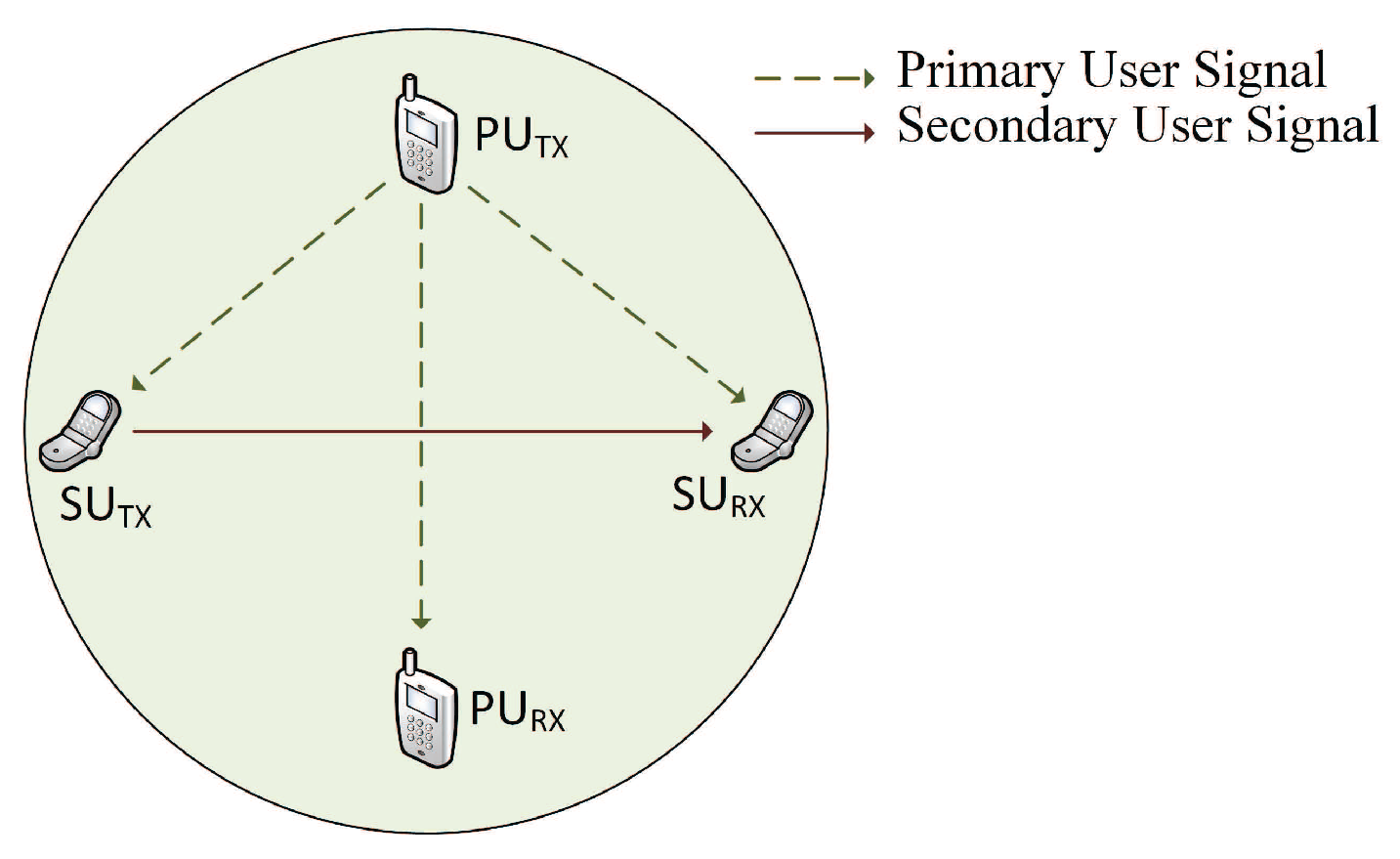
The system model considers a pair of SUs operating within the range of PU transmitter, as shown in Figure 2. The bold line represents the signal of the SU channel, whereas the dashed line denotes the PU signal. For simplicity, a single channel is assumed on which both the PU and the SU operate. The SU senses the channel and extracts the features from the input signal, then concatenates the residual energy as a percentage. The trained SVM puts the observation into one of the predefined classes. The SU transmission decision, along with the transmission power, is selected based on the output of the SVM. If the decision is for no transmission, the SU will wait for the next time slot to start sensing the channel again.

The sensing result under hypotheses $H_0$ and $H_1$ is given as follows:

$$\left\{\begin{array}{c}{H}_0:x_i=n_i,\hfill \\ H_1:x_i=s_i+n_i,\hfill \end{array}\right.$$

(1)

where $s_i$ and $n_i$ for $i=1,2,\dots ,M$ represent the received PU signal and the additive white Gaussian noise at the ith sample, respectively, and M is the total number of sensing samples in one observation obtained in a sensing slot. $H_0$ and $H_1$ denote the hypotheses in which the PU is absent and is present, respectively. The local observation of a SU node is given as

$$Y=\sum _{i=1}^M{\left|x_i\right|}^2.$$

(2)

For a large value of sensing samples per observation, for instance $M\ge 300$, the received signal energy can be approximated as a Gaussian distribution, given as follows:

$$Y\sim \left\{\begin{array}{cc}N(M,2M),\hfill & H_0,\\ N(M(1+{\gamma }_p),2M(1+2{\gamma }_p),\hfill & H_1,\end{array}\right.$$

(3)

where ${\gamma }_p$ denotes the SNR of the PU signal. The probability of false alarm, $P_f$ (the probability of falsely detecting the PU’s presence when the PU is not present), and the probability of detection, $P_d$ (the probability of detecting the PU’s presence when the PU is actually present), for given energy threshold, $\lambda$, of sensing signal are given as follows:

$$\begin{array}{c}{P}_f=P(Y>\lambda |H_0)=Q\left(\frac{\lambda -M}{\sqrt{2M}}\right),\hfill \\ P_d=P(Y>\lambda |H_1)=Q\left(\frac{\lambda -M({\gamma }_p+1)}{\sqrt{2M(2{\gamma }_p+1)}}\right),\hfill \end{array}$$

(4)

where $Q(.)$ is the complementary cumulative distribution of a standard Gaussian, defined as $Q\left(x\right)={\int }_x^{+\infty }{e}^{-t^2/\phantom{-t^{2}2}2}dt/\phantom{{\int }_x^{+\infty }{e}^{-t^2/\phantom{-t^{2}2}2}dt\sqrt{2\pi }}\sqrt{2\pi }$.

2.1. Sensing Result Classification

The classification patterns of the received signal energy range and the residual energy of the SU node are given in Figure 3a,b, respectively. The $H_0$ hypothesis on the PU’s received signal is classified into k discrete regions, $re{g}_n$, by using k reliability thresholds, ${\lambda }_n=\{P_{dn},P_{fn}\}$, where $n=1,2,\dots ,k$. The region under hypothesis $H_1$ can be considered a single class in which the SU does not execute transmission. The threshold for which $n=k$ defines the boundary between the $H_1$ and $H_0$ hypotheses. Let the residual energy of the SU node be denoted by $E_r$. The residual energy of the node is also classified into $j+1$ discrete regions by using thresholds ${\alpha }_m$, where $m=1,2,\dots ,j$, as shown in Figure 3b.

The predefined classes or hypotheses for k reliability thresholds of the received signal and j thresholds of the battery can be given as

$$\begin{array}{c}{C}_0\left\{\begin{array}{c}Y>{\lambda }_k\forall {\alpha }_j\hfill \\ orY>{\lambda }_{k-1}\&\&E_r<{\alpha }_{j-1}\hfill \\ \dots \hfill \\ orY>{\lambda }_1\&\&E_r<{\alpha }_1\hfill \end{array}\right.\hfill \\ C_1\left\{\begin{array}{c}{\lambda }_k>Y>{\lambda }_{k-1}\&\&E_r>{\alpha }_j\hfill \\ or{\lambda }_{k-1}>Y>{\lambda }_{k-2}\&\&{\alpha }_j>E_r>{\alpha }_{j-1}\hfill \\ \dots \hfill \\ or{\lambda }_1>Y\&\&{\alpha }_1>E_r\hfill \end{array}\right.\hfill \\ C_2\left\{\begin{array}{c}{\lambda }_{k-1}>Y>{\lambda }_{k-2}\&\&E_r>{\alpha }_j\hfill \\ or{\lambda }_{k-2}>Y>{\lambda }_{k-3}\&\&{\alpha }_j>E_r>{\alpha }_{j-1}\hfill \\ \dots \hfill \\ orY<{\lambda }_1\&\&{\alpha }_2>E_r>{\alpha }_1\hfill \end{array}\right.\hfill \\ \dots \hfill \\ Cn\left\{Y<\right.{\lambda }_1\&\&E_r>{\alpha }_j\hfill \end{array}$$

(5)

where $C_0,C_1,\dots ,Cn$ are labels of n different classes.

Furthermore, it is assumed that the SU node is equipped with the functionality of non-redio frequency energy harvesting. The harvested energy, denoted as $e_h$, arrives in the form of discrete packets, such that energy harvested at time t is given as

$$e_h\left(t\right)\in E_h=\left\{e_1^h,e_2^h,\dots ,e_{max}^h\right\}.$$

(6)

The residual energy of the SU node at time $t+1$ is obtained as $E_r(t+1)=E_r\left(t\right)-e^{con}\left(t\right)+e_h\left(t\right)\le B$, where $e^{con}\left(t\right)$ is the consumed energy packets at time t, and B is the battery capacity of the SU node. The harvested energy packets in the SU are assumed to follow a Poisson process with mean ${\mu }_{eh}$, given by

$$P(e_h\left(t\right)=q)=e^{-{\mu }_{eh}}\frac{{\left({\mu }_{eh}\right)}^q}{q!}.$$

(7)

The objective is to choose the transmission power of the SU node based on the energy level of the sensed PU signal and the residual energy in the SU node’s battery. The higher the sensed energy level, the lower the transmission power of the SU node. In contrast, the higher the residual energy in the SU node’s battery, the higher the transmission power of the SU node. The reason is that the higher sensed energy means a higher probability of the PU’s presence, and hence, lower transmission power should be selected to reduce interference with the PU signal by the SU, because it can be a missed detection where the SU node did not detect the presence of the PU. The selection of lower transmission power when the residual energy of the SU node is low increase the energy efficiency of the system, and thus, increase the capacity. The simulation results verify these statements by achieving higher throughput under the proposed scheme, compared to conventional systems where only two classes are considered, i.e., $H_0$ and $H_1$.

The total number of classes is obtained using k regions of the received signal energy and j discrete levels of the battery. The classification obtained by dividing the received signal energy into five regions (including the region under hypothesis $H_1$), i.e., $k=4$, and quantizing the residual energy of the SU node into four levels, i.e., $j=3$, is given in

Table 1. Classification with proposed scheme for $k=4$ regions of sensed signal energy range and $j=3$ levels of residual energy in SU battery.

Residual Energy Level	$\mathit{re}{\mathit{g}}_5$	$\mathit{re}{\mathit{g}}_4$	$\mathit{re}{\mathit{g}}_3$	$\mathit{re}{\mathit{g}}_2$	$\mathit{re}{\mathit{g}}_1$
$L_1$	$C_0$	$C_0$	$C_0$	$C_0$	$C_1$
$L_2$	$C_0$	$C_0$	$C_0$	$C_1$	$C_2$
$L_3$	$C_0$	$C_0$	$C_1$	$C_2$	$C_3$
$L_4$	$C_0$	$C_1$	$C_2$	$C_3$	$C_4$

. The $L_i$ for $i=1,2,3,4$ and $re{g}_i$ for $i=1,2,\dots ,5$ represent the discrete residual energy levels and quantized received signal energy levels, respectively. $Ci$ is the output class of the classifier categorized based on the residual energy and received signal energy. $C_0$ is the class when the SU node does not transmit. In $re{g}_5$ of the received signal energy, the SU does not transmit irrespective of the residual energy in the SU node’s battery; refer to Table 1. This region is considered under the hypothesis $H_1$ where the detection probability of PU is high. For regions of the received signal energy other than $re{g}_5$, the SU node selects transmission power $P_{Ti}$ according to the output class, $Ci$, of the classifier, which is based on the residual energy of the SU node. Class $C_1$ refers to the scenario in which the SU node selects the lowest transmission power, $P_{T1}$. Similarly, transmission power $P_{T2}$, chosen in case of $C_2$, is comparatively higher than $P_{T1}$ and lower than $P_{T3}$ (selected under $C_3$). The highest value of transmission power, $P_{T4}$, is selected when the classifier gives output of $C_4$, the class in which the received signal energy is in the lowest region but the residual energy is at the highest level. The four values of transmission power, $P_{Ti}$ for $i\in \{1,2,3,4\}$, respective to each output class, i.e., $Ci$ for $i\in \{1,2,3,4\}$, are predefined by the system. The SU node selects one of the four values according to the output of the classifier. The selection of transmission power values is also critical to improving the performance of the system. These values can be obtained by considering different parameters of the environment, including the distance between SU nodes, the distance of the SU transmitter from the PU nodes, etc. However, this consideration is outside the scope of current study. In this work, the fixed values of transmission power for different classes are used with respect to energy consumption packets in the simulations. The transmission power can be obtained as the ratio of the energy consumed to the transmission time, $P_{Ti}=e_i^{con}/\phantom{e_i^{con}{\tau }_r}{\tau }_r$, where ${\tau }_r$ is the transmission duration, obtained as ${\tau }_r=T-{\tau }_s$ for T and ${\tau }_s$ being the total duration of one time slot and the sensing time duration, respectively.

The capacity of the SU link for the ith class is obtained as

$$c_i=W{log}_2\left(1+{\gamma }_{si}\right),$$

(8)

where ${\gamma }_{si}=P_{Ti}/\phantom{P_{Ti}{N}_0}{N}_0$ is the SNR of the SU channel, W is the bandwidth and $N_0$ is noise power. The throughput obtained in the ith class classification can be given as

$$R_i=\frac{T-{\tau }_s}{T}{c}_i.$$

(9)

2.2. Classifier Characteristics

The well-known machine learning-based algorithm called a support vector machine is used to classify the received signal. Primarily, an SVM is designed to deal with two-class classification problems. A linear hyperplane is drawn as a decision surface between two classes of data points. The nearest data points to the decision boundary of each class are known as support vectors, hence the name support vector machine. In fact, the decision boundary is drawn by taking support vectors into account. The optimization problem of the SVM in obtaining the decision boundary for training data ${\left\{(x_i,l_i)\right\}}_{i=1}^N$ is given as follows [31]:

$$\begin{array}{c}min\Phi \left(\mathbf{w}\right)=\frac{1}{2}∥\mathbf{w}∥\hfill \\ \mathrm{such}\mathrm{that}\hfill \\ l_i({\mathbf{w}}^T{x}_i+b)\ge 1\mathrm{for}i=1,2,\dots ,N.\hfill \end{array}$$

(10)

A test input, ${\mathbf{x}}_j$, can be classified using the following decision function:

$$f\left({\mathbf{x}}_j\right)=sign\left(\sum _i{\alpha }_{i}K({\mathbf{x}}_i,{\mathbf{x}}_j)+b\right).$$

(11)

To apply an SVM for multi-class classification problems, the SVM can be used in a one-versus-rest approach. In this approach, h different SVMs are utilized for an h-class classification problem. The hth SVM is trained with data points, referring to the hth class as a positive class and referring to the data points from the remaining $h-1$ classes as a negative class. The final decision is made according to the classifier with the highest score in the positive class.

2.3. Kernel Functions

In classification problems where it is not possible for a linear hyperplane to distinguish between the two classes, a kernel function, denoted as $K(x,y)$, is used to transform the data from input space to a higher dimensional space where it is possible for a linear hyperplane to differentiate the data elements of two classes. The three kernel functions utilized in this work are given in

Table 2. Kernel functions for arbitrary input vectors $\mathbf{x}$ and $\mathbf{y}$.

Kernel Function	$\mathit{K}(\mathbf{x},\mathbf{y})$
Linear Function	${\mathbf{x}}^T\mathbf{y}+c$
Polynomial Function	${({\mathbf{x}}^T\mathbf{y}+1)}^p$
Radial-Basis Function	$exp\left(-\frac{{∥\mathbf{x}-\mathbf{y}∥}^2}{2{\sigma }^2}\right)$

for arbitrary input vectors $\mathbf{x}$ and $\mathbf{y}$.

2.4. Features Extraction

Increases in the dimensionality of input observations to an SVM greatly affect the performance of the classifier. To reduce the dimensionality, input to the SVM is given in the form of features extracted from the input observation that reflect the characteristics of the observation. Feature extraction and feature selection have significant importance in machine learning-based classification and regression problems. This improves performance of the classifier in terms of computational cost, accuracy, and delay time to solve the problem. In this work, the three statistical features extracted from the input sensed signal are given in

Table 3. Features extracted from received signal of PU.

$X_1=10\times {\left(\frac{1}{M}{\displaystyle \sum _{i=1}^M}{s}_i\right)}^{10}.$

$X_2=\frac{1}{M}{\displaystyle \sum _{i=1}^M}{s}_i^2.$

$X_3=\sqrt{{\left({\displaystyle \sum _{i=1}^q}{s}_i\right)}^3};q\le M,s_{i+1}\ge s_i.$

. The first feature $X_1$ is obtained by taking power 10 of the mean value of sensed signal and then multiplying by 10. The constant value 10 in power and multiplication terms are used such that the small difference in the mean values of different classes is magnified, resulting in better classification accuracy. A variation in this constant value can affect the performance of classifier, however satisfactory results are obtained with the given value. The second feature $X_2$ is simply the mean of the squared elements of the received signal. The third feature $X_3$ is obtained by taking the root of the cubic sum of the first q elements of the received signal arranged in descending order. To the best of the authors’ knowledge, this work is the first to adopt this feature.

3. Simulation Results

Simulations are performed using MATLAB (R2017a, The MathWorks Inc., Natick, MA, USA, 2017). A dataset for each training and testing phase, having 500 and 2000 observations, respectively, is generated using Equation (1). First, the activity of PU was generated with a 50% probability of the PU’s presence. Then, the PU’s signals were generated for each of the generated activity of PU. The percentage residual energy values of the node are generated randomly from 0 to 100 with a uniform distribution. Finally, each observation was labeled based on the probability of detection obtained from the sensed signal and the residual energy of node. This means that, in each training and testing dataset, the distribution of observations over the five classes was not fixed and were obtained randomly. The observations in training dataset, which is consisted of the three features (given in Table 3) extracted from input received signal concatenated with the residual energy of the node, are labeled as classes $C_0$ to $C_4$, as shown in Figure 1. In testing phase, the harvested energy is added with a Poisson distribution to the residual energy of SU node in each iteration. After updating the residual energy, the received signal is classified again using the updated residual energy of SU node. The recent classification result of SVM obtained using the updated observation is then used to obtain the channel capacity. In this way, the throughput of the channel is obtained for each iteration. The simulation steps are summarized as follows: the SVM-based classifier is trained in a one-versus-rest approach using training dataset consisting of 500 labeled input observations. Each observation is obtained by concatenating the three statistical features extracted from received signal and the residual energy of the node as the fourth feature. The testing dataset of 2000 unlabeled observations is used to analyze performance.

Table 4. Simulation Parameters.

Name	Symbol	Value
One Slot Duration	T	100 ms
Sensing Time	${\tau }_s$	3 ms
Bandwidth	W	1 MHz
Sensing Samples	M	300
Training Observations		500
Testing Observations		2000
Prob. of Detection of Reliability Thresholds	$P_{d1},P_{d2},P_{d3},P_{d4}$	0.95, 0.9, 0.85, 0.8
Residual Energy Classification Thresholds	${\alpha }_1,{\alpha }_2,{\alpha }_3$	25, 50, 75(%)
Reference Energy	$E_{ref}$	20 Packets
Energy Difference	$E_{diff}$	5 Packets
Kernel Function		Polynomial
k-fold Cross-validation		4

lists the values of simulation parameters assumed in the experiment.

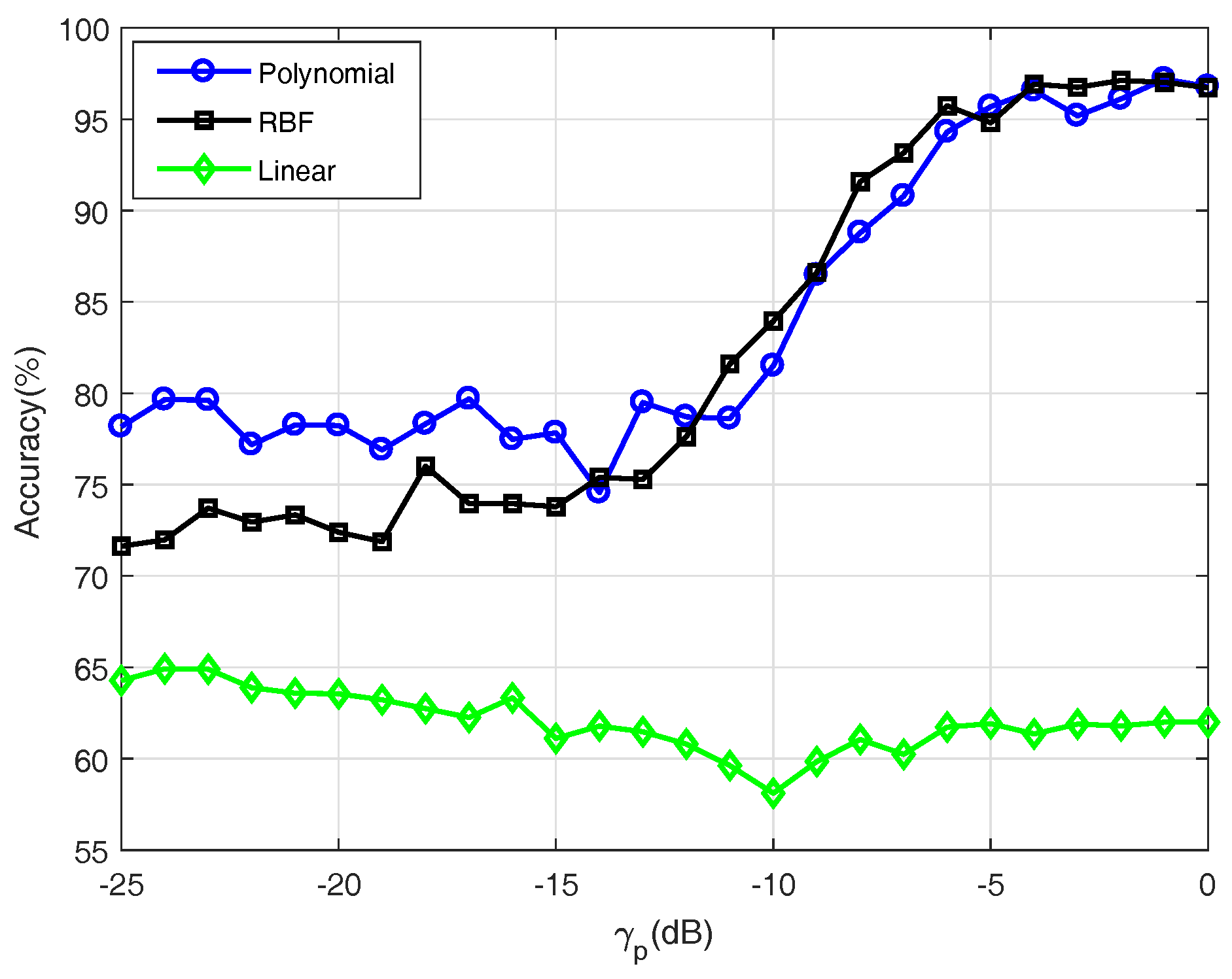
The performance of the classifier is analyzed using accuracy, defined as the ratio of correct classifications to the number of total test observations. Figure 4 shows the accuracy comparison of three separate classifiers trained with three kernel functions (linear, RBF, and polynomial) applied in proposed multi-hypothesis scheme of spectrum sensing versus the SNR of the PU, ${\gamma }_p$, ranging from −25 dB to 0 dB. The classifiers trained with the RBF and the polynomial kernel function always performed better than the linear kernel function, which attained accuracy between 60% and 65%, irrespective of ${\gamma }_p$. The former mentioned two classifiers followed a similar trend of improving accuracy with an increase in ${\gamma }_p$. The minimum accuracy of 72% was achieved for ${\gamma }_p=-25\mathrm{dB}$ with the RBF kernel. The accuracy varied slightly when ${\gamma }_p$ increased to −12 dB. Further increases in ${\gamma }_p$ rapidly increased accuracy to 95% to 96% for ${\gamma }_p=-5\mathrm{dB}$. Additional raise in ${\gamma }_p$ from −5 dB does not affect the performance of the classifier considerably. The polynomial kernel–based classifier followed a trend similar to that of the RBF kernel, although the accuracy ranged from 75% to 80% for ${\gamma }_p=-25\mathrm{dB}\sim -12\mathrm{dB}$. The better performance of polynomial kernel function-based classifier, compared to the counter two kernel functions-based classifiers, at a low ${\gamma }_p$, lets it be used for further simulations, although it achieved comparable accuracy at higher ${\gamma }_p$ to the RBF kernel function-based classifier.

Figure 5 shows the achievable average throughput versus the total battery capacity of the SU node. Based on the output of the classifier, transmission power varied in each iteration. Then, the corresponding throughput was calculated according to Equation (9). The term average refers to the calculation in two phases. In the first phase, the average value of the throughput was calculated as the ratio of total achieved throughput (obtained by a single node in 10,000 iterations) to the number of opportunities for transmission. The result was then averaged on the total number of observations, which is 2000. The resultant values were used to obtain Figure 5.

The throughput was achieved for two values of ${\gamma }_p=-15\mathrm{dB}$ and ${\gamma }_p-5\mathrm{dB}$. The results of the proposed algorithm are compared to conventional two-class spectrum sensing ($H_0$ and $H_1$) in two scenarios. First, the max transmission power (the transmission power for $C_4$) in the proposed scheme is used for transmission in $H_0$ sensing result, labeled as Max Tx Power in the figure. Secondly, the minimum transmission power (used for $C_1$) in the proposed scheme is used for transmission in conventional two-class spectrum sensing when PU is sensed absent, labeled as Min Tx Power. Note that a similar classifier with similar characteristics and matching sizes of training and testing datasets is used in all scenarios. Min Tx Power outperformed Max Tx Power in terms of throughput for a limited battery capacity because of a higher number of transmission attempts. However, we can see from the figure that the proposed scheme achieves efficient performance compared to the other two scenarios. In all cases the throughput follows an almost constant trend when battery capacity is increased from 1500 packets in SU node. The reason is the usage of energy harvesting equipped-SU node and the fixed 10,000 number of iterations for SU to sense and transmit. When the battery capacity is low, the battery is emptied with a few number of transmission executions. Then the SU node waits to store enough residual energy for transmission using energy harvesting function. With increase in the battery capacity (such as above 1500 packets), there is low chances of SU to be out of battery. At these higher battery capacity values, the throughput is affected by the number of attempts of transmissions rather than the battery capacity. The theoretical results of the proposed scheme are also given in the Figure 5. In the paper, theoretical results in machine learning mainly deal with a type of inductive learning called supervised learning. In supervised learning, an algorithm is given samples that are labeled in some useful way. To get a theoretical performance of the proposed scheme, which can be considered as “upper bound” of the performance the proposed scheme, we utilize the following steps: First, a vector containing the activity of PU (H) is generated with a 50% probability of the PU’s presence. Then, the PU’s signals are generated for each of the activities of PU. The residual energy in percentage of the SU node is generated randomly with a uniform distribution. Finally, each observation (a vector containing three features extracted from PU signal concatenated with residual energy) was labeled based on the $P_d$ of the signal and the residual energy of node. After labeling, the capacity of channel is obtained for each label of the observation. In each iteration, the residual energy of SU is updated by deducting the energy consumed for transmission and adding the harvested energy with a Poisson distribution. The correct class labels of observations are used to obtain the theoretical results whereas the output labels of SVM are used in simulation results. Consequently, there is a difference between the theoretical and simulation results, as illustrated in the figure. The difference between the theoretical and simulation results of proposed scheme is higher for ${\gamma }_p=-15$ dB as compared to ${\gamma }_p=-5$ dB. The reason to this statement is that the accuracy of SVM is comparatively lower for ${\gamma }_p=-15$ dB. The higher number of miss-classifications when ${\gamma }_p=-15$ dB lead to a higher difference from theoretical results as compared to ${\gamma }_p=-5$ dB.

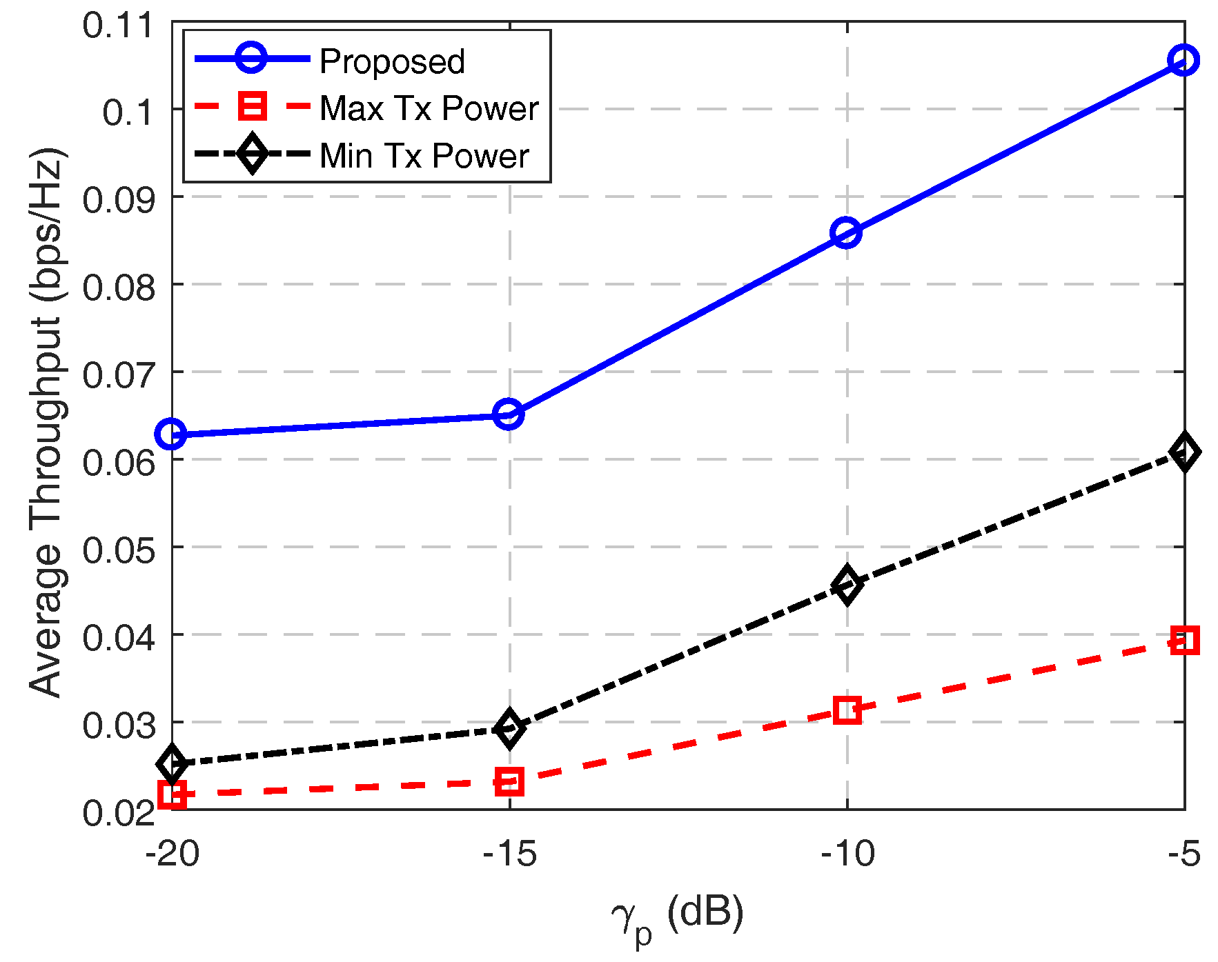
A comparison of average throughput versus ${\gamma }_p$ is presented in Figure 6. All scenarios follow a similar trend with a slight increase in throughput from −20 to −15 dB for ${\gamma }_p$. Further increases in ${\gamma }_p$ also increase the slope of the graph. As shown in the figure, the throughput achieved in the proposed scheme is much higher than Max Tx Power and Min Tx Power scenarios for all ranges of ${\gamma }_p$. The total battery capacity, B, was kept at 100 packets to obtain these results.

The relation of average throughput to the reference energy consumption is demonstrated in Figure 7. The reference energy is the maximum energy consumed for maximum power transmission under the proposed scheme. For instance, the transmission energy consumed for $C_1$, $C_2$, $C_3$, and $C_4$ was 5, 10, 15, and 20 packets, respectively, when the reference energy was 20 packets, whereas the transmission energies were 20 and 5 packets for Max Tx Power and Min Tx Power, respectively. The details on reference consumption energy to the energy consumed in different scenarios and classes can be understood from

Table 5. The relation of reference energy consumption to energy consumed in each transmission scenario.

Reference Energy Packets		20	25	30	35
Proposed Scheme	$C_4$	20	25	30	35
	$C_3$	15	20	25	30
	$C_2$	10	15	20	25
	$C_1$	5	10	15	20
Max Tx Power		20	25	30	35
Min Tx Power		5	10	15	20

.

The results shown in the figure strengthen the claim that the proposed scheme achieves better performance, compared to Max Tx Power and Min Tx Power scenarios. With the battery capacity at 100 packets, the average throughput decreases with an increase in the reference consumption energy. However, the proposed scheme shows improved results compared to Max Tx Power and Min Tx Power for both ${\gamma }_p=-15\mathrm{dB}$ and ${\gamma }_p=-5\mathrm{dB}$.

Discussion

In this work, five classes are considered under the proposed scheme. No transmission occurred for C0, which can occur due to a higher level of received signal energy or due to low residual energy in the SU node (refer to Table 1). Increasing or decreasing the total number of classes with increases or decreases in the number of reliability thresholds for the received signal energy and/or the number of quantized levels of residual energy in the node will affect the performance of the classifier remarkably, and hence, the achievable throughput. Increases in the number of output classes, to some extent, may improve the performance of the system with a cost of high computation, because increasing the number of classes will increase the number of classifiers used in the one-versus-rest approach. However, improvement in performance is not guaranteed, because an increase in the number of classes also increases the complexity of the classifier. Furthermore, a delay in the classification of classifier will increase. Hence, a trade-off occurs between achievable throughput and computational costs or between throughput and delay.

Moreover, the machine learning-based classifiers perform better than statistical spectrum sensing techniques such as matched filtering, energy detector, spectral correlation, etc., with a higher computational cost. More energy and resources are used to learn and train the classifier. The sensor nodes or SUs are equipped with batteries of limited capacity. Therefore, the training phase of classifier is performed by the fusion center (FC) and the optimized parameters of trained classifiers are provided to the SU nodes. These SU nodes utilize given parameters for classification of the sensed signal. If any maintenance or update of the training or learning is needed, the FC will do the job and then provide the updated parameters to SU nodes. In this way, the workload of the SU nodes is reduced to conserve energy.

Furthermore, the classification performance of a system using ML-based classifier is affected significantly by the number and combination of features extracted from the input signal. For a good performance, the features should be used such that the properties of signals from different classes are reflected. Nevertheless, the length of input vector should be as minimal as possible to reduce the computational cost of the system. Therefore, using the lowest possible number of good features may improve the classification performance of the classifier. In this work, the proposed combination of three features improves the classification accuracy of SVM-based classifier for multi-hypothesis spectrum sensing in cognitive radio networks. This claim is verified by the simulation results. Obviously, the performance of the classifier may improve further by using better features combination. However, it is needed to explore more to obtain such a combination of features. A feature selection scheme can be utilized to do the job of selecting the best combination of features from a feature pool with a cost of computational complexity. However, it is out of scope of this paper and can be reserved as a further work.

4. Conclusions

Machine learning-based algorithms have recently attracted attention in spectrum sensing for cognitive radio networks. The main advantage of these algorithms over conventional spectrum sensing algorithms is their heuristic nature and independence from needing prior information about the environment. An SVM-based algorithm is utilized in spectrum sensing with multi-class hypotheses. The transmission power of the SU node varies according to the received signal energy level and the stored energy in the battery. Altering the transmission power based on the probability of the PU’s presence aids in reducing interference with the PU’s activity; transmission with low power, if the stored energy in the battery is low, increases the number of transmission intervals or, alternatively, the throughput of the SU node. Input to the SVM is given in the form of four-dimensional vectors: three features extracted from the received signal concatenated with the percentage of residual energy. The SVM with a polynomial kernel function and the proposed features was able to achieve almost 75% accuracy, even in a low SNR range from −25 dB to −15 dB. This performance improved to 95% accuracy with an increase in the SNR up to −5 dB. In addition, the simulation results show that throughput improved compared to conventional two-class hypothesis-based spectrum sensing.

References

- Ian, P. What exactly is… cognitive radio? IEEE Commun. Eng. Mag. 2005, 3, 42–43. [Google Scholar]
- Benedetto, F.; Giunta, G.; Guzzon, E.; Renfors, M. Detection of Hidden Users in Cognitive Radio Networks. In Proceedings of the 2013 IEEE 24th International Symposium on Personal, Indoor and Mobile Radio Communications (PIMRC’13), London, UK, 8–11 September 2013; pp. 2296–2300. [Google Scholar]
- Engleman, R.; Abrokwah, K.; Dillon, G.; Foster, G.; Godfrey, G.; Hanbury, T.; Lagerwerff, C.; Leighton, W.; Marcus, M.; Noel, R. Report of the Spectrum Efficiency Working Group; Federal Communications Commission Spectrum Policy Task Force: Washington DC, WA, USA, 2002. Available online: https://www.fcc.gov/sptf/files/SEWGFinalReport_1.doc (accessed on 15 January 2018).
- Walko, J. Cognitive radio. IEE Rev. 2005, 51, 34–37. [Google Scholar] [CrossRef]
- Benedetto, F.; Giunta, G.; Guzzon, E.; Renfors, M. Effective Monitoring of Freeloading User in the Presence of Active User in Cognitive Radio Networks. IEEE Trans. Veh. Technol. 2014, 63, 2443–2450. [Google Scholar] [CrossRef]
- Oo, T.Z.; Tran, N.H.; Dang, D.N.M.; Han, Z.; Le, L.B.; Hong, C.S. OMF-MAC: An opportunistic matched filter-based MAC in cognitive radio networks. IEEE Trans. Veh. Technol. 2016, 65, 2544–2559. [Google Scholar] [CrossRef]
- Atapattu, S.; Tellambura, C.; Jiang, H. Energy detection based cooperative spectrum sensing in cognitive radio networks. IEEE Trans. Wirel. Commun. 2011, 10, 1232–1241. [Google Scholar] [CrossRef]
- Chen, Y. Improved energy detector for random signals in gaussian noise. IEEE Trans. Wirel. Commun. 2010, 9, 558–563. [Google Scholar] [CrossRef]
- Zhang, D.; Chen, Z.; Ren, J.; Zhang, N.; Awad, M.K.; Zhou, H.; Shen, X.S. Energy-Harvesting-Aided Spectrum Sensing and Data Transmission in Heterogeneous Cognitive Radio Sensor Network. IEEE Trans. Veh. Technol. 2017, 66, 831–843. [Google Scholar] [CrossRef]
- Tuan, P.V.; Koo, I. Throughput maximisation by optimising detection thresholds in full-duplex cognitive radio networks. IET Commun. 2016, 10, 1355–1364. [Google Scholar] [CrossRef]
- Jang, W.M. Blind Cyclostationary Spectrum Sensing in Cognitive Radios. IEEE Commun. Lett. 2014, 18, 393–396. [Google Scholar] [CrossRef]
- Xue, D.; Ekici, E.; Vuran, M.C. Cooperative Spectrum Sensing in Cognitive Radio Networks Using Multidimensional Correlations. IEEE Trans. Wirel. Commun. 2014, 13, 1832–1843. [Google Scholar] [CrossRef]
- Yücek, T.; Arslan, H. Spectrum Characterization for Opportunistic Cognitive Radio Systems. In Proceedings of the IEEE Military Communications Conference, Washington, DC, USA, 23–25 October 2006; pp. 1–6. [Google Scholar]
- Yucek, T.; Arslan, H. A survey on spectrum sensing algorithms for cognitive radio. IEEE Commun. Surv. Tutor. 2009, 11, 116–130. [Google Scholar] [CrossRef]
- Ghasemi, A.; Sousa, E.S. Spectrum Sensing in Cognitive Radio Networks: Requirements, Challenges and Design Trade-offs. IEEE Commun. Mag. 2008, 46. [Google Scholar] [CrossRef]
- Jiang, C.; Zhang, H.; Ren, Y.; Han, Z.; Chen, K.; Hanzo, L. Machine Learning Paradigms for Next-Generation Wireless Networks. IEEE Wirel. Commun. 2017, 24, 98–105. [Google Scholar] [CrossRef]
- Azmat, F.; Chen, Y.; Stocks, N. Analysis of Spectrum Occupancy using Machine Learning Algorithms. IEEE Trans. Veh. Technol. 2016, 65, 6853–6860. [Google Scholar] [CrossRef]
- Harrington, P. Machine Learning in Action; Manning Publications Co.: Greenwich, CT, USA, 2012. [Google Scholar]
- Patan, K. Artificial Neural Networks for the Modelling and Fault Diagnosis of Technical Processes; Springer: Berlin/Heidelberg, Germany, 2008. [Google Scholar]
- Wang, F.; Zhen, Z.; Wang, B.; Mi, Z. Comparative Study on KNN and SVM Based Weather Classification Models for Day Ahead Short Term Solar PV Power Forecasting. Appl. Sci. 2018, 8, 28. [Google Scholar] [CrossRef]
- Elangovan, K.; Tamilselvam, Y.K.; Mohan, R.E.; Iwase, M.; Nemoto, T.; Wood, K. Fault diagnosis of a reconfigurable crawling-rolling robot based on support vector machines. Appl. Sci. 2017, 7, 1025. [Google Scholar] [CrossRef]
- Sun, J.; Sun, F.; Fan, J.; Liang, Y. Fault Diagnosis Model of Photovoltaic Array Based on Least Squares Support Vector Machine in Bayesian Framework. Appl. Sci. 2017, 7, 1199. [Google Scholar] [CrossRef]
- Jan, S.U.; Lee, Y.-D.; Shin, J.; Koo, I. Sensor Fault Classification Based on Support Vector Machine and Statistical Time-Domain Features. IEEE Access 2017, 5, 8682–8690. [Google Scholar] [CrossRef]
- Park, S.; Hong, D. Achievable throughput of energy harvesting cognitive radio networks. IEEE Trans. Wirel. Commun. 2014, 13, 1010–1022. [Google Scholar] [CrossRef]
- Sultan, A. Sensing and transmit energy optimization for an energy harvesting cognitive radio. IEEE Wirel. Commun. Lett. 2012, 1, 500–503. [Google Scholar] [CrossRef]
- Liang, Y.C.; Zeng, Y.; Peh, E.C.; Hoang, A.T. Sensing-Throughput Tradeoff for Cognitive Radio Networks. IEEE Trans. Wirel. Commun. 2008, 7, 1326–1336. [Google Scholar] [CrossRef]
- Awe, O.P.; Lambotharan, S. Cooperative spectrum sensing in cognitive radio networks using multi-class support vector machine algorithms. In Proceedings of the 2015 9th International Conference on Signal Processing and Communication Systems (ICSPCS), Cairns, QLD, Australia, 14–16 December 2015. [Google Scholar]
- Thilina, K.M.; Choi, K.W.; Saquib, N.; Hossain, E. Machine Learning Techniques for Cooperative Spectrum Sensing in Cognitive Radio Networks. IEEE J. Sel. Areas Commun. 2013, 31, 2209–2221. [Google Scholar] [CrossRef]
- Zhang, D.; Zhai, X. SVM-Based Spectrum Sensing in Cognitive Radio. In Proceedings of the 2011 7th International Conference on Wireless Communications, Networking and Mobile Computing, Wuhan, China, 23–25 September 2011; pp. 1–4. [Google Scholar]
- Hou, F.; Chen, X.; Huang, H.; Jing, X. Throughput performance improvement in cognitive radio networks based on spectrum prediction. In Proceedings of the 2016 16th International Symposium on Communications and Information Technologies (ISCIT), Qingdao, China, 26–28 September 2016; pp. 655–658. [Google Scholar]
- Haykin, S. Neural Networks: A Comprehensive Foundation; Prentice-Hall, Inc.: Upper Saddle River, NJ, USA, 1999. [Google Scholar]
Figure 1.
Flowchart of the proposed scheme: (a) the training phase; and (b) the testing phase.
Figure 2.
System model considering a pair of secondary users (SUs) operating in the range of primary users (PUs).
Figure 3.
Classification pattern of: (a) received signal energy sensed by SU; and (b) residual energy of SU node.
Figure 4.
Comparison of the accuracy of the support vector machine (SVM)-based classifiers trained with linear, radial-basis function (RBF), and polynomial kernel functions applied in proposed scheme.
Figure 5.
Average throughput versus battery capacity of SU node.
Figure 6.
Average throughput versus PU SNR for battery capacity, B = 100 of SU node.
Figure 7.
Average throughput versus reference consumption energy with battery capacity, B = 100 of SU node.