Evaluation of the Implicit Gradient-Enhanced Regularization of a Damage-Plasticity Rock Model


Unit for Strength of Materials and Structural Analysis, Institute of Basic Sciences in Engineering Sciences, University of Innsbruck, Technikerstr 13, A-6020 Innsbruck, Austria
*
Author to whom correspondence should be addressed.
Appl. Sci. 2018, 8(6), 1004; https://doi.org/10.3390/app8061004
Submission received: 11 May 2018
/
Revised: 28 May 2018
/
Accepted: 29 May 2018
/
Published: 20 June 2018
(This article belongs to the Special Issue Computational Methods for Fracture)
Abstract
:In the present publication, the performance of an implicit gradient-enhanced damage-plasticity model is evaluated with special focus on the prediction of complex failure modes such as shear failure. Hence, it complements studies on predominant mode I failure frequently found in the literature. To this end, an implicit gradient-enhanced damage-plasticity rock model is presented and validated by means of 2D and 3D finite element simulations of both laboratory tests on intact rock specimens as well as a large-scale structural benchmark related to failure of rock mass. Thereby, a wide range of loading conditions comprising unconfined and/or confined, tensile and/or compressive stress states is considered. The capability of the gradient-enhanced rock model for representing the mechanical response objectively with respect to the finite element discretization and realistically compared to measurement data is assessed. It is shown that complex failure modes and the respective load–displacement curves are predicted in a mesh-insensitive manner.
1. Introduction
The appropriate representation of complex failure modes of cohesive-frictional materials in numerical simulations is of great interest for many engineering applications, which include, among others, geotechnical applications characterized by material failure playing a dominant role in the overall structural response [1,2]. A prominent example of material failure under highly confined stress states is given in the context of tunnel construction: During the construction of deep tunnels, high geostatic stresses in the surrounding rock mass are redistributed in consequence of the excavation process [3,4]. Depending on the quality of the surrounding rock mass, the installed supporting measures, and the type of excavation process, those stress redistributions can lead to damage in the rock mass, often accompanied by the transition from the rock mass as a continuum to rock blocks moving towards the tunnel center with localized shear bands indicating the sliding interfaces. It follows that an adequate representation of such failure phenomena by means of advanced constitutive models is of great importance and a prerequisite for the risk assessment of potential structural collapse.
Constitutive models based on the combination of the theory of plasticity and continuum damage mechanics, simply denoted as damage-plasticity models, provide a powerful framework for describing inelastic deformations, hardening and softening material behavior, as well as stiffness degradation due to damage. They are well suited for the description of cohesive-frictional materials such as concrete, rock, and soils, since different types of material failure, e.g., cracking in tension, crushing in compression, or failure under mixed stress states, can be described in a realistic manner [5]. On the basis of damage-plasticity models, the material behavior is described in terms of mere continuum relations, i.e., constitutive relations describing the behavior of an infinitesimal material point. However, softening material behavior, described in terms of continuum models, exhibits several theoretical deficiencies, as reported and summarized in [6]:
- the softening process zone is infinitesimally small;
- at structural level, snapback behavior due to the infinitesimally small softening zone is observed;
- the dissipated energy during the failure process is zero due to the infinitesimal zone in which energy is dissipated.
In a mathematical sense, those issues are related to the loss of ellipticity of the initial boundary value problem (IBVP) in static and quasi-static analyses. In finite element analyses, those deficiencies lead to mesh-dependent results, commonly referred to as a pathological mesh sensitivity. Failure patterns like cracks tend to localize into the smallest possible bandwidth, i.e., usually a single layer of finite elements, and upon mesh refinement the localization zone is decreasing to an arbitrarily small domain. Accordingly, the obtained results are not objective with respect to the finite element mesh, i.e., the results are sensitive with respect to the numerical discretization scheme. In the past decades, several techniques to overcome these deficiencies in numerical simulations have been proposed, for instance the crack band approach based on a mesh-adjusted softening modulus [7], nonlocal approaches of the integral type [8], models based on the Cosserat continuum [9], viscoplastic formulations [10], phase field models [11], and explicit and implicit gradient-enhanced formulations [12].
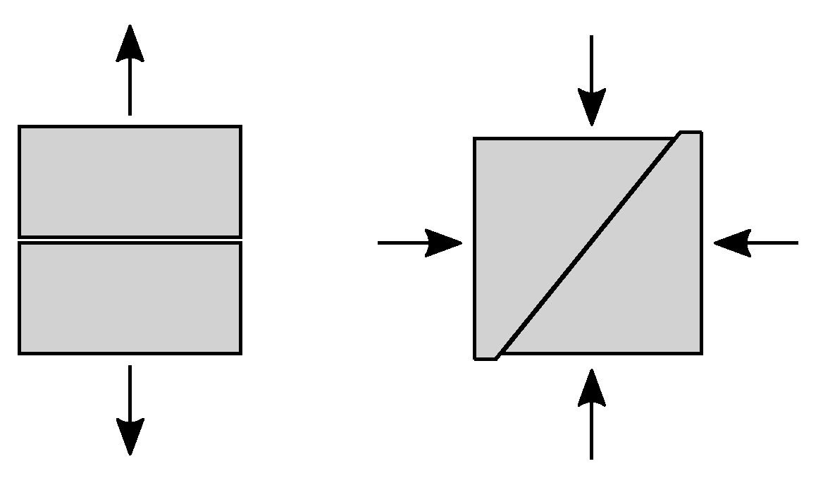
Among these approaches, models based on implicit gradient-enhanced formulations by now form a well-established branch in the literature due to their computational efficiency and numerical stability [12]. Numerous implicit gradient-enhanced damage and plasticity models have been proposed in recent years [13,14,15,16,17,18,19,20,21], and their performance has been demonstrated based on different examples of material failure. In particular, many gradient-enhanced models have been developed explicitly for concrete [13,16,17,21], and special attention has been paid to the proper representation of cracking under predominantly tensile stress states [17,22]. However, while cracking in tension (cf. Figure 1 left) is an important failure mode for concrete structures, considerably less attention was paid to shear failure (cf. Figure 1 right), i.e., pure mode II failure, or mixed failure under confined stress states. In fact, many of the available models have been validated based on examples of mode I failure, and often it is tacitly assumed that they perform equally well for more complex failure modes.
The apparent gap in the literature on the assessment of gradient-enhanced models for describing such complex failure modes motivates a systematic investigation of a gradient-enhanced constitutive model applied to different types of material failure. To this end, in the present contribution, a gradient-enhanced damage-plasticity model for rock is proposed and evaluated. This model is considered as a representative for a wide class of gradient-enhanced damage-plasticity models. The model is based on the damage-plasticity model by Unteregger et al. [24], and its damage formulation is extended following the implicit gradient-enhanced approach proposed by Poh and Swaddiwudhipong [17]. Based on numerical examples involving complex failure modes, the capability of the model to capture different types of material failure in a realistic and objective manner in finite element simulations will be demonstrated.
The remainder of the paper is organized as follows: In Section 2, the original damage-plasticity model for intact rock and rock mass, proposed in [24,25], is briefly summarized. In Section 3, the implicit gradient-enhancement of the rock model is presented, and the numerical implementation into a finite element framework is discussed. Section 4 covers numerical simulations of laboratory tests including wedge splitting tests as well as triaxial compression tests and triaxial extension tests with various levels of confining pressure. Additionally, a benchmark example of tunnel excavation will be presented, and the representation of complex failure modes in an objective manner with respect to the employed finite element mesh will be demonstrated. Finally, in Section 5, the paper is closed with a summary and a discussion on recommended future research activities.
2. Damage-Plasticity Model for Intact Rock and Rock Mass
The damage-plasticity model for intact rock and rock mass, denoted as RDP model in the following, was proposed originally for intact rock in [24] and was further extended to rock mass in [25] by incorporating empirical down-scaling factors to account for the influence of discontinuities according to [26,27,28].
The RDP model is based on the theory of plasticity formulated in the effective stress space combined with continuum damage mechanics. The stress-strain relation is expressed as
in which describes the nominal Cauchy stress tensor (force per total area), the scalar isotropic damage parameter ranging from 0 (undamaged material) to 1 (fully damaged material), the fourth order elastic stiffness tensor, the total strain tensor, and the plastic strain tensor. The effective stress tensor (force per undamaged area) is linked to the nominal stress tensor by
The elastic domain is bounded by the smooth Hoek–Brown yield criterion [29,30] formulated in the Haigh–Westergaard coordinates of the effective stress tensor, i.e., the mean stress , the deviatoric radius , and the Lode angle in the deviatoric plane . In addition, a stress-like hardening variable is incorporated leading to the definition of the yield function as
Therein, is the uniaxial compressive strength, is the friction parameter, is the Willam–Warnke function to describe the shape of the yield surface in deviatoric planes, and parameters and s are empirical down-scaling factors to account for discontinuities in rock mass, the latter depending on the geological strength index and the disturbance factor D according to [26]. A default value for the eccentricity e of 0.51 is proposed in [24]. For representing material behavior of intact rock, and s are equal to 1.
The flow rule for describing the evolution of plastic strains is defined in the effective stress space as
with denoting the consistency parameter and the non-associated plastic potential function expressed as
Therein, volumetric plastic flow is controlled by dilatancy parameters and . In the expression for , is calibrated from experimental results (uniaxial tension, uniaxial compression, and triaxial compression tests) of intact rock specimens and is determined from
such that the lateral plastic strain rate in uniaxial tension is zero. Uniaxial tensile strength ftu is calculated from (3) as
Hardening material behavior is described by means of the stress-like internal variable
which is conjugate to the strain-like hardening variable and contains the yield stress in uniaxial compression . The evolution law for the strain-like hardening variable is given as
in which is the norm of the gradient of the plastic potential function with respect to effective stress, denotes the reduction of the Young’s modulus of rock mass compared to intact rock [26] ranging from 0 (completely disintegrated) to 1 (intact rock), and is a measure for describing hardening ductility, defined as
with . In (10), model parameters , , , , and control the hardening behavior. They are calibrated by experimental data from uniaxial tension, uniaxial compression, and triaxial compression tests. In [24,25], default values of and are suggested in absence of respective experimental data.
Damage is provoked when the hardening variable attains its maximum value of 1. At this stage, the scalar isotropic damage parameter starts evolving dependent on the strain-like internal softening variable . This relation is described by means of an exponential softening law as
with the softening modulus controlling the slope of the softening curve. The rate of the strain-like internal softening variable is computed from the volumetric part of the plastic strain rate as
Therein, the softening ductility measure
accounts for the influence of multi-axial stress states on the softening behavior, with describing the compressive part of the volumetric plastic strain rate. Model parameters and are calibrated from experimental data of uniaxial compression and triaxial compression tests. Again, in absence of respective experimental data for parameters and , default values of and are proposed in [24].
3. Implicit Gradient-Enhancement of the Damage-Plasticity Model for Intact Rock and Rock Mass
Softening material behavior leads to an ill-posed initial boundary value problem and consequently to pathological mesh-sensitivity in finite element simulations. As a remedy, in [24], the crack band approach was employed for the RDP model. While the crack band approach is a rather simple regularization technique, it is also characterized by a number of shortcomings, which are addressed in [31]. Motivated by those deficiencies, in the following, a more sophisticated regularization technique based on the implicit gradient-enhanced formulation [32] is presented. To this end, the approach by Poh and Swaddiwudhipong [17] proposed for a damage-plasticity model for concrete and based on the gradient of the internal softening variable, is adopted. By incorporating the gradient of an internal variable into the constitutive relations, nonlocality is introduced. Thus, the mechanical response of a material point does not exclusively depend on its local state, but is also influenced by the state in its neighborhood.
Nonlocality is incorporated by replacing the local softening variable by a weighted softening variable in the exponential damage law (11), which is expressed as
Therein, the softening modulus is a material parameter. The weighted softening variable is calculated from a combination of the local softening variable and its nonlocal counterpart as
in which m denotes a weighting parameter. Choosing m larger than 1 yields the over-nonlocal formulation [33] to achieve full regularization of the problem, as proven in [34]. Furthermore, by ensuring that can only increase, damage is considered as an irreversible process [35].
According to the implicit approach, the field of the nonlocal softening variable , henceforth simply denoted as the nonlocal field, is defined implicitly as the solution of a higher-order partial differential equation. Adopting the formulation by Poh and Swaddiwudhipong [17], for the description of the nonlocal field a second order partial differential equation is employed as
in which l denotes a length scale parameter defining the radius of nonlocal interaction, is the Laplace operator and represents the local softening variable of (12), and is the spatial domain occupied by the body under consideration. Equation (16) is a screened-Poisson equation, commonly denoted as the Helmholtz equation in the context of implicit gradient-enhanced formulations [12,36]. It is apparent that nonlocality affects only the damage part of the model and the plasticity part of the RDP model remains local.
As suggested in [32,37], homogeneous Neumann boundary conditions are assumed as on the entire boundary of the domain with the normal vector to the boundary . This boundary condition was interpreted in [38] in the context of phase-field models enforcing cracks to occur perpendicular to the boundary.
The set of governing equations is completed by the equilibrium equation
in which is the vector of body forces. For the boundary conditions, the surface traction vector on and prescribed displacements on are assumed.
Partial differential Equations (16) and (17) form a fully coupled system with the unknown displacement vector and the nonlocal field , which is solved by means of the finite element method. To this end, the weak form is formulated, which is subsequently discretized in space and in time. To obtain the weak form, the set of partial differential equations is multiplied by test functions for the displacement field and for the nonlocal field. Integration over the domain, application of the divergence theorem, incorporation of the infinitesimal strain , and consideration of on yields the weak form of the IBVP expressed in Voigt notation as
The displacement field and the nonlocal field are approximated over the domain using a Bubnov-Galerkin approach as
in which contains the shape functions and are column vectors of the nodal unknown parameters, both expressed in the global form employing the standard assembly procedure, with standing for the displacement field and the nonlocal field , respectively. The infinitesimal strain and the gradient of the nonlocal field are discretized as
with the strain-displacement matrix and the row vector of the spatial derivatives of the shape functions for the field of the nonlocal softening variable , again both expressed in the global form employing the standard assembly procedure. It follows that the shape functions for both fields must meet the requirement of -continuity.
Due to the nonlinear and path-dependent character of the IBVP, an incremental solution procedure is employed. For the incremental solution procedure, a discrete (pseudo-)time interval is considered such that the body under consideration is in equilibrium at time . At this time, the nodal values and , the stress and the internal variables and are known. An incremental load is applied such that the traction vector and the vector of body forces at time are prescribed as and . The updated variables of the constitutive relations at time , i.e., , , , are evaluated by means of a stress-update algorithm, employing an implicit integration scheme following the return-mapping approach [39] for the plastic regime and a subsequent explicit evaluation of the damage part. Finally, the incremental discretized weak form is obtained as
Since Equations (24) and (25) must hold for arbitrary kinematically admissible test functions and , they can be recast into the residual format as
with and denoting internal and external force vectors related to the displacement field, and is the residual vector for the nonlocal field. Due to the nonlinear dependence of the system of Equations (26) and (27) on the unknown nodal solution vector
an iterative Newton–Raphson solution procedure is employed. The nodal unknowns at time in the i-th iteration step are composed of , where has to be determined. Linearization of Equations (26) and (27) at the state with the initial guess of the nodal unknowns yields the iterative procedure for the correction of the nodal unknowns for time after the i-th iteration step
with the submatrices of the system matrix given as
in which , , and are the consistent tangent stiffness submatrices. They represent the derivatives of the constitutive relations consistent with the numerical algorithm for integrating the path-dependent rate constitutive equations, which is essential for the full Newton–Raphson scheme in order to preserve a quadratic rate of convergence. Due to the non-associated plastic flow rule of the RDP model and the coupling of the displacement field and the nonlocal field, the system matrix is unsymmetric. From the computed correction of the nodal unknowns , the updated solutions of the incremental nodal unknowns, and the total nodal unknowns are obtained.
4. Numerical Study
The aim of the present numerical study is to evaluate the performance of the implicit gradient-enhanced RDP model for predicting the mechanical response of structures, involving the softening behavior of rock in a realistic and mesh-insensitive manner for a wide range of loading conditions. To this end, a numerical study is presented, related to both laboratory tests and practical applications. It consists of the following parts:
- 2D modeling of mode I failure in wedge splitting tests on Indiana limestone performed by Brühwiler and Saouma [40],
- 3D modeling of shear failure in triaxial compression tests performed by Blümel [41] on specimens of Innsbruck quartz phyllite, considering the influence of confined stress states attaining the compressive meridian of the yield surface,
- 3D numerical simulations of triaxial extension tests performed on the same type of specimens, investigating the influence of confined stress states attaining the tensile meridian of the yield surface, and
- 2D numerical simulations of the excavation of a deep tunnel in Innsbruck quartz phyllite rock mass leading to the formation of shear bands in the vicinity of the tunnel for demonstrating the capability of the gradient-enhanced RDP model to predict failure of a complex structure.
4.1. Modeling of Mode I Failure, Demonstrated by Analyzing Wedge Splitting Tests on Indiana Limestone
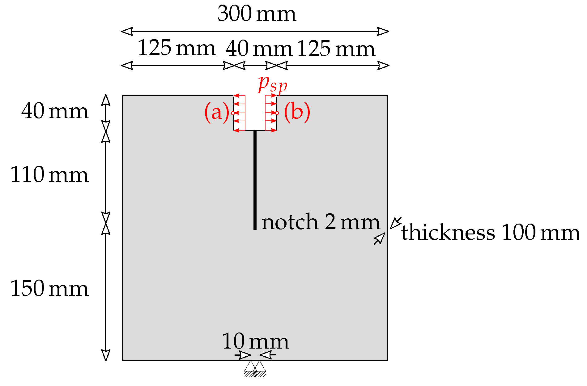
In a first step, the capability of the gradient-enhanced RDP model for predicting mode I failure is assessed. To this end, the experimental study of wedge splitting tests on Indiana limestone performed by Brühwiler and Saouma [40] is considered. The investigated specimen is illustrated in Figure 2.
During the experimental test, the splitting force was applied by a vertically driven wedge, exerting a pressure against roller bearings that were mounted on both sides of the groove in the specimen. The vertical (machine) force and the crack mouth opening displacement (CMOD) were recorded, and the latter was controlled during the experimental test. The energy conjugate force to the CMOD, the splitting force , was calculated from the vertical force considering the geometry of the wedge and neglecting any frictional effects. In total, 5 tests were performed, but in [40] detailed load–displacement curves were presented only for Test 3. To investigate the degradation of the stiffness of the specimen during crack propagation, several loading/unloading cycles were performed.
The experimental test is simulated by means of a two-dimensional finite element model assuming plane stress conditions. According to Figure 2, the specimen is supported in the vertical direction at the bottom center over a width of 10 mm and in the horizontal direction at midpoint. The splitting force , transmitted by the wedge, is approximated by the pressure acting on the lateral groove faces. The simulation is performed in a displacement-driven manner by controlling the CMOD (i.e., the relative horizontal displacement between points (a) and (b) in Figure 2) during the loading and unloading cycles. The material parameters for representing the Indiana limestone were determined by a best fit with the recorded experimental results. In the present example of mode I failure, only few parameters have a significant influence on the results: E = 22000 MPa, , , , , , , , , , and . For the weighting parameter m, any value larger than 1 is sufficient to ensure full regularization of the problem by avoiding spurious localization of plastic strain [33]. A discussion on the influence of the weighting parameter m may be found in [42] for an integral-type nonlocal model, where, however, for parameter , an overestimation of the energy dissipation close to a notch was demonstrated. This non-physical effect was also observed by the authors with increasing influence for larger values of m. Thus, parameter m is chosen just slightly larger than 1, in accordance with proposed values from the literature [17,43]. For the remaining model parameters e, , , , , and , the default values summarized in Section 2 are employed. From Equation (7), the uniaxial tensile strength is calculated as .
To investigate the influence of the finite element discretization on the predicted results, different meshes are employed: Three structured meshes with fully integrated 4-node quadrilateral elements and element sizes of 5 mm, 1 mm, and 0.5 mm in the vicinity of the expected crack path, as well as one unstructured mesh with the same element type and an element size of 1 mm along the crack path. Accordingly, the element size of 5 mm is slightly larger compared to the assumed length scale l of 4 mm for the coarse mesh and considerably smaller for the medium and fine mesh. The purpose of the unstructured mesh is to investigate a potential bias of the crack pattern by following the grid lines of the finite element mesh, since mesh-biased crack paths have been observed for smeared crack models based on the crack band approach [44].
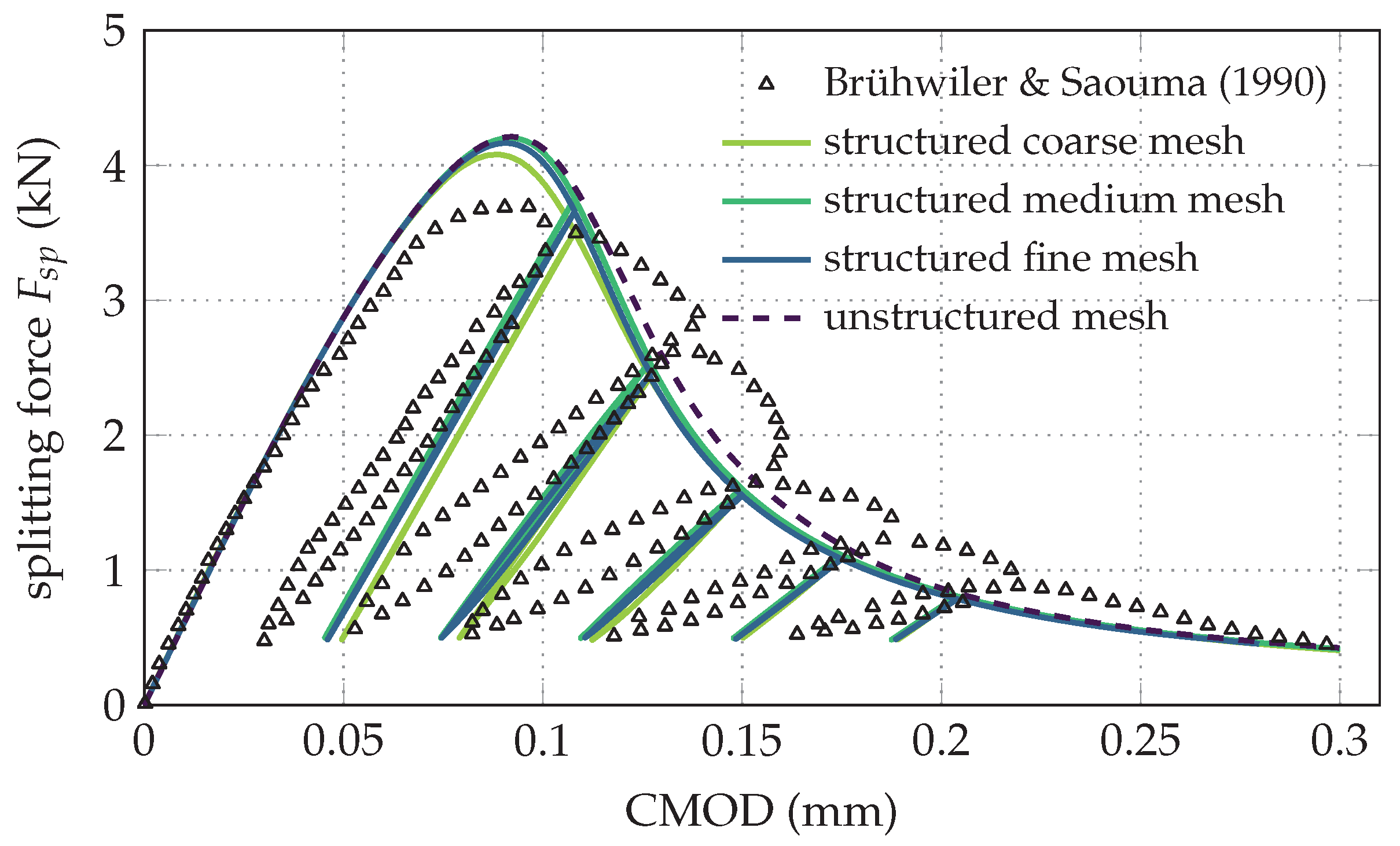
In Figure 3, the resulting load–displacement curves, i.e., splitting force versus CMOD, are shown for the considered experimental test and the numerical simulations. It can be concluded that the qualitative shape of the experimentally obtained curve is approximated quite well in the numerical simulations.
Regarding the influence of the finite element mesh on the computed load–displacement curves, a slight difference between the predicted response based on the structured coarse mesh and the one based on the structured medium mesh is visible. This is explained by the rough approximation of the gradient of the nonlocal field by the coarse mesh. In contrast, almost identical load–displacement curves are obtained for the structured medium and the structured fine mesh, confirming that the gradient of the nonlocal field can be resolved sufficiently by those meshes. The unstructured mesh results in a similar load–displacement curve, demonstrating that the gradient-enhanced approach is not biased by the orientation of the finite element mesh.
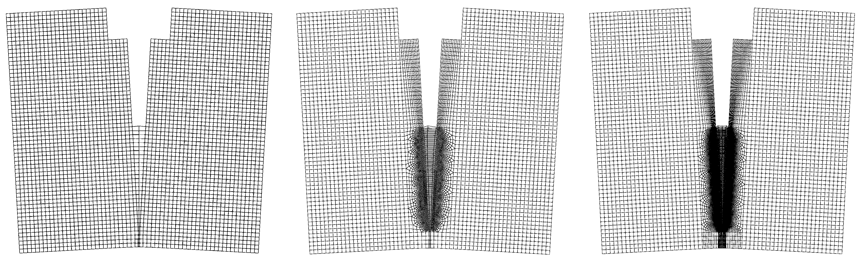
The computed deformation of the specimen is depicted in Figure 4 for the three structured meshes. By increasing the splitting force during the numerical simulations, the tensile strength of the material is attained at first in the elements directly below the notch; consequently, damage is initiated. This leads to large, localized deformations in this region. Upon further loading, the increase of these deformations reflects the opening of a crack, propagating towards the bottom of the specimen. This is represented by the gradient-enhanced damage-plasticity approach in a smeared manner. The width of the damage zone is related to the length scale parameter l (cf. (16)). Furthermore, it can be seen that an identical symmetrical response with respect to the vertical axis of symmetry is obtained for all three structured meshes.
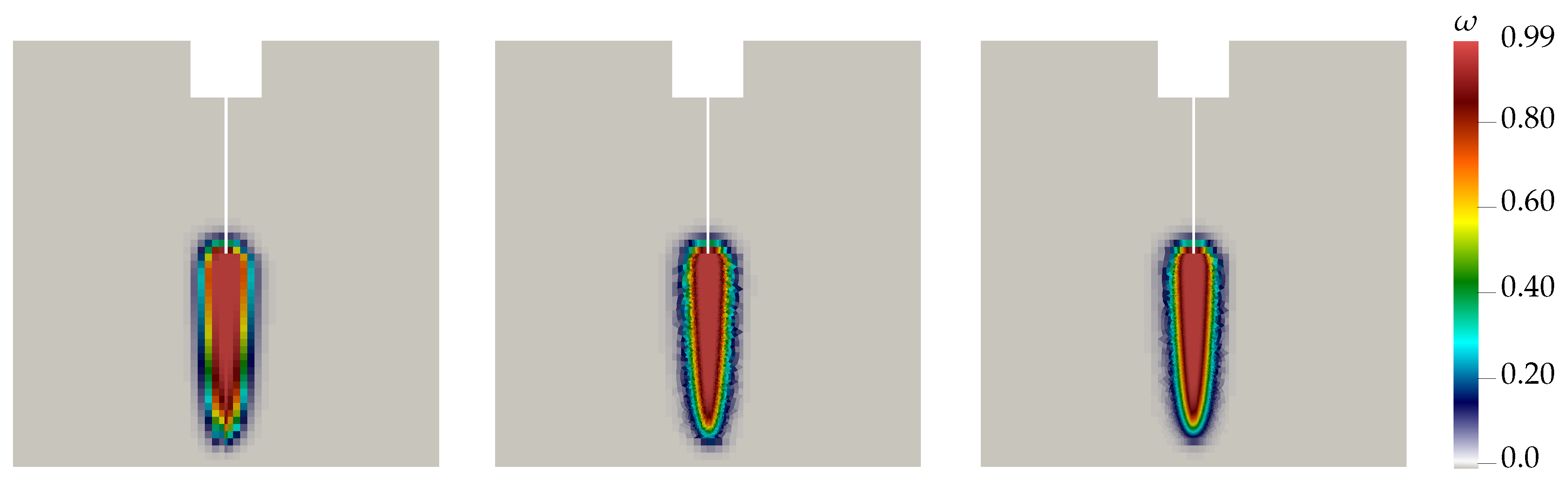
In Figure 5, the distribution of the damage variable computed for the three structured meshes is plotted at a CMOD = 0.3 mm. It is visible that damage is also accumulated slightly above the notch tip. This is a consequence of the diffusive character of the gradient-enhanced formulation. Furthermore, the present gradient-enhanced RDP model with the constant length scale l predicts a rather broad zone of complete damage (red region in Figure 5). In fact, this behavior does not represent damage localizing into a discrete macrocrack, and has been addressed in [45,46]. However, comparison of the predicted damage distributions for the different meshes demonstrates mesh-insensitivity of the obtained failure patterns. Figure 3 and Figure 6 show an identical load–displacement curve and identical deformation pattern and damage distribution computed by means of the unstructured mesh, which underlines the capability of the gradient approach to produce mesh-insensitive results.
4.2. Modeling of Shear Failure, Demonstrated by Analyzing Triaxial Compression Tests on Innsbruck Quartz Phyllite
In a second step, the performance of the gradient-enhanced RDP model for predicting shear failure under confined stress states attaining the compressive meridian of the yield surface is assessed. To this end, numerical simulations of triaxial compression tests on specimens of Innsbruck quartz phyllite performed by Blümel [41] are conducted.
For the experimental program, intact rock specimens with a diameter of 35 mm and a height of 70 mm were taken from drill cores sampled at the construction site of the Brenner Base Tunnel. A series of triaxial compression tests with different levels of confining pressures (uniaxial compression), 12.5 MPa, 25.0 MPa, and 37.5 MPa was conducted. The experiments were performed in a sequential manner: Firstly, the confining pressure was applied, resulting in an initial hydrostatic stress state in the specimen, and subsequently, an axial pressure was applied displacement-driven up to failure. The mechanical response in the post-peak regime was also recorded.
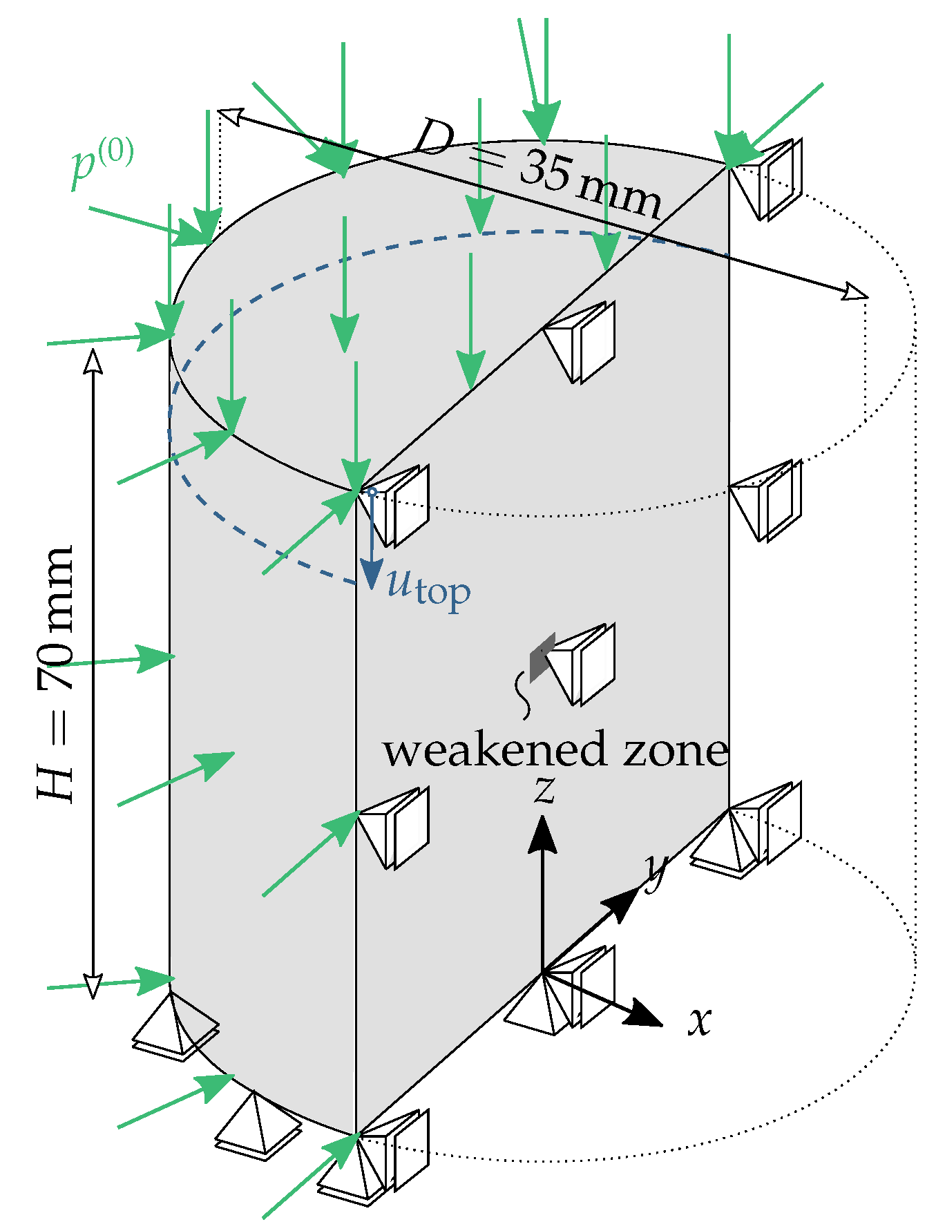
Finite element simulations of triaxial compression tests are often performed in an approximate manner. Commonly, such tests are simplified as single element tests in which the non-homogeneous deformation of the specimen observed in the experiments cannot be captured, or by two-dimensional models in which three-dimensional effects are neglected, e.g., [24,47,48,49]. By contrast, in the present study, a three-dimensional finite element model is employed in order to capture the three-dimensional deformations in a realistic manner. The numerical model with the prescribed boundary conditions and loads is illustrated in Figure 7. Since the failure mode is expected to be symmetric with respect to a vertical plane through the center axis of the specimen, symmetry is exploited by considering only one half of the specimen. By analogy to the experimental tests, the numerical simulations are performed in two sequential steps: firstly, the specimen is supported vertically at the bottom face and the confining pressure is applied; secondly, the axial loading is applied by imposing a uniform vertical displacement at the top of the specimen.
The specimens are discretized with 20-node hexahedral elements employing reduced numerical integration. For both the displacement field and the nonlocal field, quadratic shape functions are used. To analyze potential mesh-sensitivity of the gradient-enhanced RDP model, three different structured finite element meshes are examined. A coarse mesh with 828 elements (an element size of 4 mm), a medium mesh with 5950 elements (an element size of 2 mm), and a fine mesh with 13,160 elements (element size of 1.5 mm) are employed. To trigger localized failure, at the center of the specimen, a small zone of slightly weakened elements is introduced, as indicated in Figure 7. In the numerical simulations, snapback behavior may occur, i.e., a simultaneous decrease of the load and the displacement after attaining the peak load. At this stage, displacement-controlled experiments become unstable. To overcome potential snapback behavior in the numerical simulations, the indirect displacement control technique [50,51] is employed. For the present example, this technique can be applied by enforcing a monotonic decrease of the vertical distance between two nodes, with each node located at one boundary of the expected shear band.
The material parameters required for the elastic-plastic part of the RDP model were identified from single element simulations, as discussed in [52]. The additional parameters for the softening regime , , l, and m are calibrated from the present numerical simulations for a best fit with the experimental results for the confining pressure of . The employed parameters for Innsbruck quartz phyllite are E = 56670 MPa, , , , , , , , , , , . For the remaining model parameters e, , , , and , the default values summarized in Section 2 are employed. The experimental results for confining pressures of , , and 25 MPa, which have not been used for calibration, serve for validation of the numerical model.
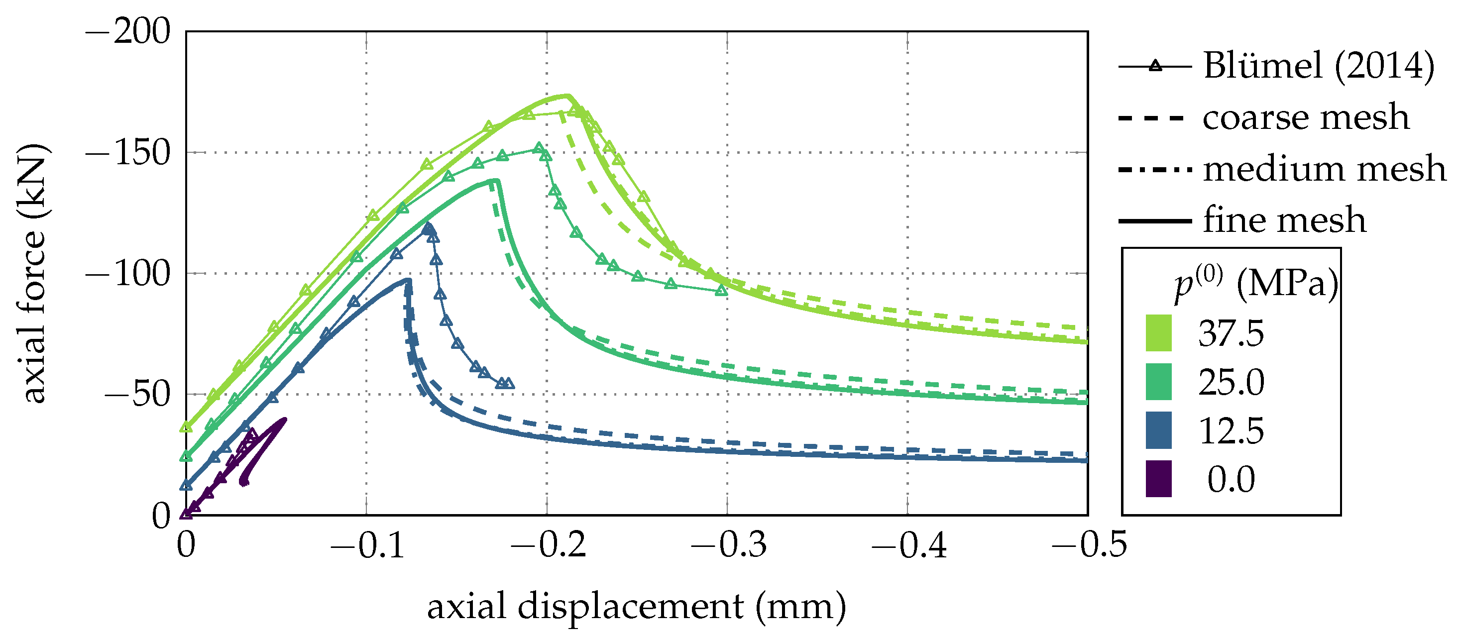
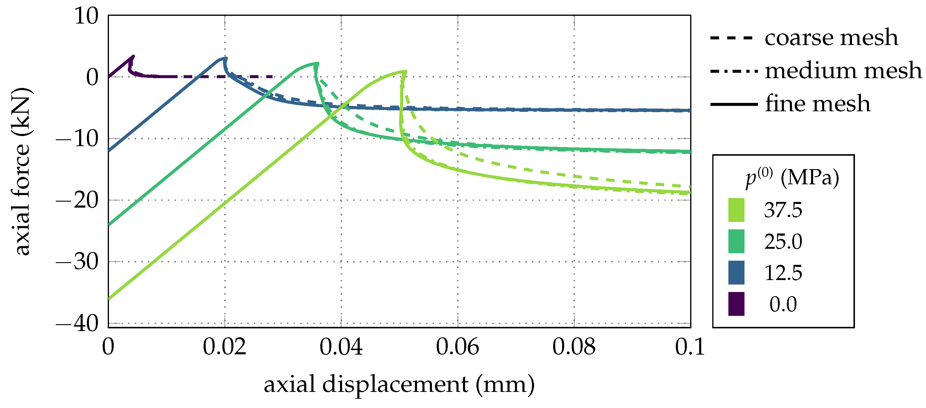
Figure 8 shows the load–displacement curves obtained from the experiments and the numerical simulations for the different confining pressures. Note that the non-zero axial force at the beginning is the consequence of the initial hydrostatic stress state due to the applied confining pressure. Expectedly, for and for the uniaxial compression test (), the experimentally obtained peak load is represented very well since the test results were used for calibration. For and 25 MPa, the peak loads are predicted satisfactorily, slightly underestimating the experimental results. The qualitative shape of the softening branch is also represented quite well. For the uniaxial compression test, no meaningful experimental results after the peak stress were recorded during the experiments. This unstable behavior is also manifested in the numerical simulations, for which strong snapback behavior is observed. The numerical results computed on the basis of the different finite element meshes reveal the capability of the gradient-enhanced RDP model to regularize the underlying IBVP: Once the mesh is sufficiently fine, mesh-insensitive load–displacement curves are obtained.
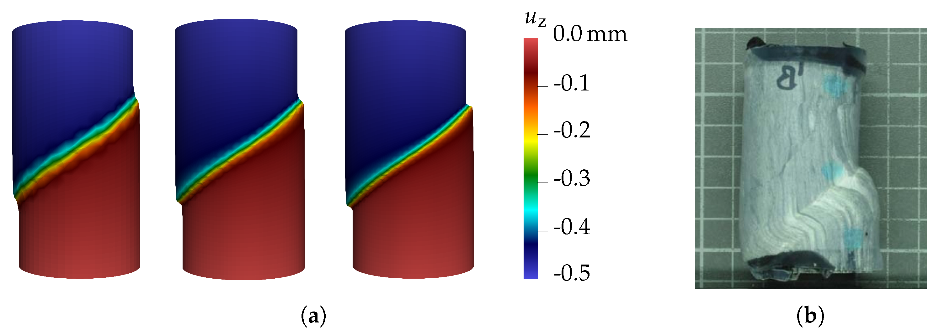
Figure 9a shows the deformed specimen with the confining pressure in the final stage of the triaxial compression tests, computed by means of the three different meshes. While the displacements in the lower and the upper part of the specimen are almost uniform, the displacements localize into a single inclined shear band in the center part of the specimen. In the experiments, localization into a shear band was found to be the dominant failure mode, as shown in Figure 9b for a specimen tested with . The formation of the shear band is also reflected by the distribution of the damage variable shown in Figure 10. Comparing the predicted damage distributions for the medium and the fine mesh confirms this distribution as insensitive with respect to the discretization.
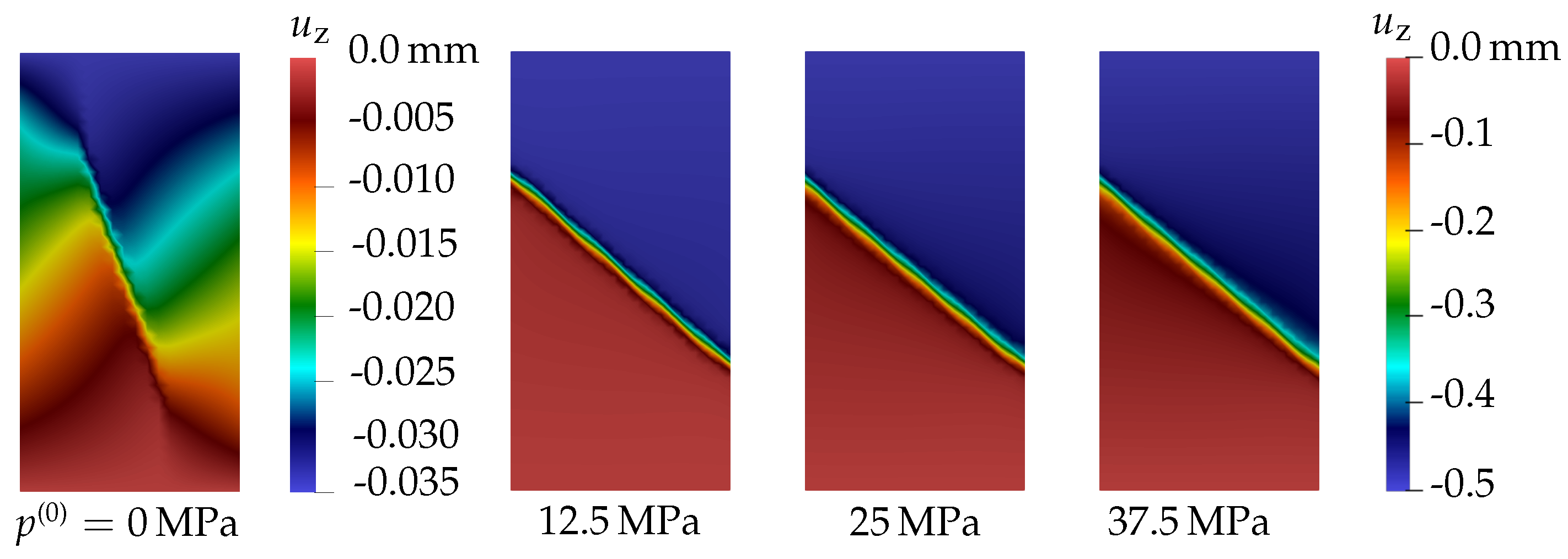
The influence of the level of confining pressure on the inclination of the shearing zone is demonstrated in Figure 11 based on the predicted distribution of the vertical displacement for , , and , respectively. For the uniaxial compression test (), the zone of localized displacements is strongly inclined. With increasing confining pressure, the inclination angle of the shear band is decreasing, which is best visible by comparing the results for and . Upon further increase of the confining pressure, the inclination of the shear band becomes slightly smaller. The represented dependence of the inclination angle on the level of confining pressure is explained by the curvature of the compressive meridian of the yield surface and of the employed plastic potential function of the RDP model.
4.3. Modeling of Shear Failure, Demonstrated by Analyzing Triaxial Extension Tests on Innsbruck Quartz Phyllite
In a third step, the ability of the model for predicting shear failure under confined stress states attaining the tensile meridian of the yield surface is demonstrated. To this end, numerical simulations of triaxial extension tests on specimens with geometric and material properties identical to those of the previously presented triaxial compression tests are performed. Similar to the triaxial compression tests, confining pressures of 0 MPa, MPa, 25 MPa, and MPa are investigated. The same finite element meshes are employed for investigating the influence of the discretization. In contrast to the triaxial compression tests, subsequent to the application of the initial hydrostatic stress state, generated by the confining pressure, a displacement in positive vertical direction is applied at the top surface of the specimens. Since for triaxial extension tests experimental results are not available, the present study focuses on the assessment of the influence of the finite element mesh on the obtained results and serves as further verification of the gradient-enhanced RDP model.
The predicted load–displacement curves are shown in Figure 12. While nearly identical results are obtained for the medium mesh and the fine mesh, the load–displacement curves for the coarse mesh are somewhat more ductile. This discrepancy indicates the coarse mesh as insufficiently fine for the accurate resolution of the gradient of the nonlocal field. Compared to the results from the triaxial compression tests, a more brittle structural response is predicted, resulting in strong snapback behavior in the post-peak regime for all three confining pressures and, in particular, for the uniaxial tension test. In contrast to the triaxial compression tests, the structural response becomes increasingly brittle as confining pressure increases, and the peak load decreases gradually. This phenomenon was also observed in experiments on Berea sandstone in [53], and it is characteristic of brittle and quasi-brittle materials.
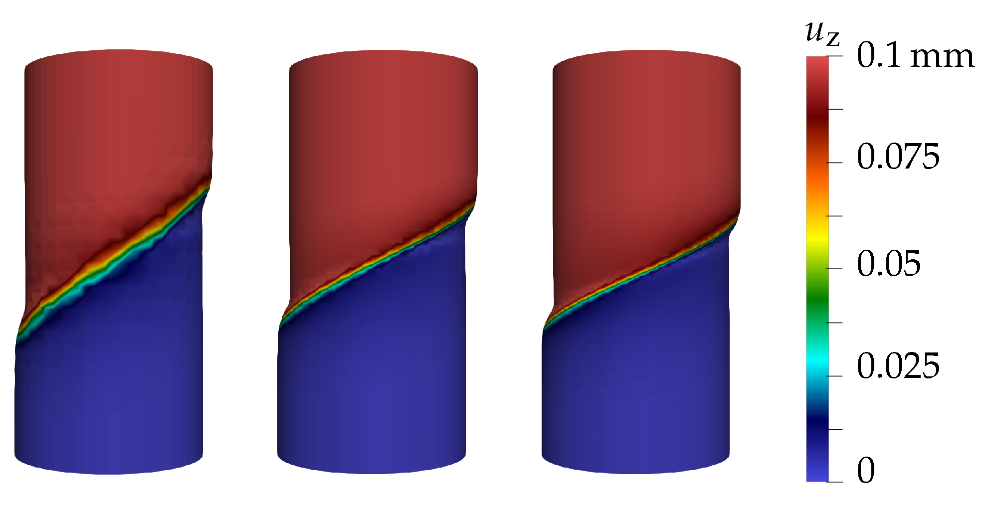
Figure 13 shows the computed deformation of the specimen for an applied axial displacement of 0.1 mm and a confining pressure of 37.5 MPa. Compared to the triaxial compression tests, a smaller inclination angle of the shear band is predicted for the medium mesh and the fine mesh, whereas for the coarse mesh a considerably steeper inclination angle of the shear band is obtained. Again, this discrepancy indicates the insufficient representation of the gradient of the nonlocal field by the coarse mesh.
4.4. Numerical Simulation of Localizing Deformations in Deep Tunnel Excavation
Finally, the performance of the gradient-enhanced RDP model for predicting the formation of multiple shear bands during the excavation of a deep tunnel is assessed. This benchmark is derived from a stretch of the Brenner Base Tunnel constructed by the drill, blast, and secure procedure, which has already been the subject of investigations in previous publications [52,54]. An analogy to the present problem can be found in the context of petrol engineering, where the formation of shear bands has been observed and reported for borehole breakout [47,55,56].
Since in this contribution the major focus is on the assessment of the gradient-enhanced rock model, the tunnel excavation is approximated by means of a simplified two-dimensional model. Supporting measures like a shotcrete shell or rock anchors are neglected. Potential time-dependent effects of the mechanical behavior of rock mass due to the excavation procedure are not considered. For the excavation of the tunnel profile by means of drill and blast, either a full-face or a sequential excavation procedure can be employed. The chosen excavation sequence may have a considerable impact on the stability of the tunnel. In this numerical model, the worst case scenario is considered by assuming full-face excavation of the circular tunnel profile without any supporting measures, which results in the maximum loading of the rock mass in the vicinity of the tunnel.
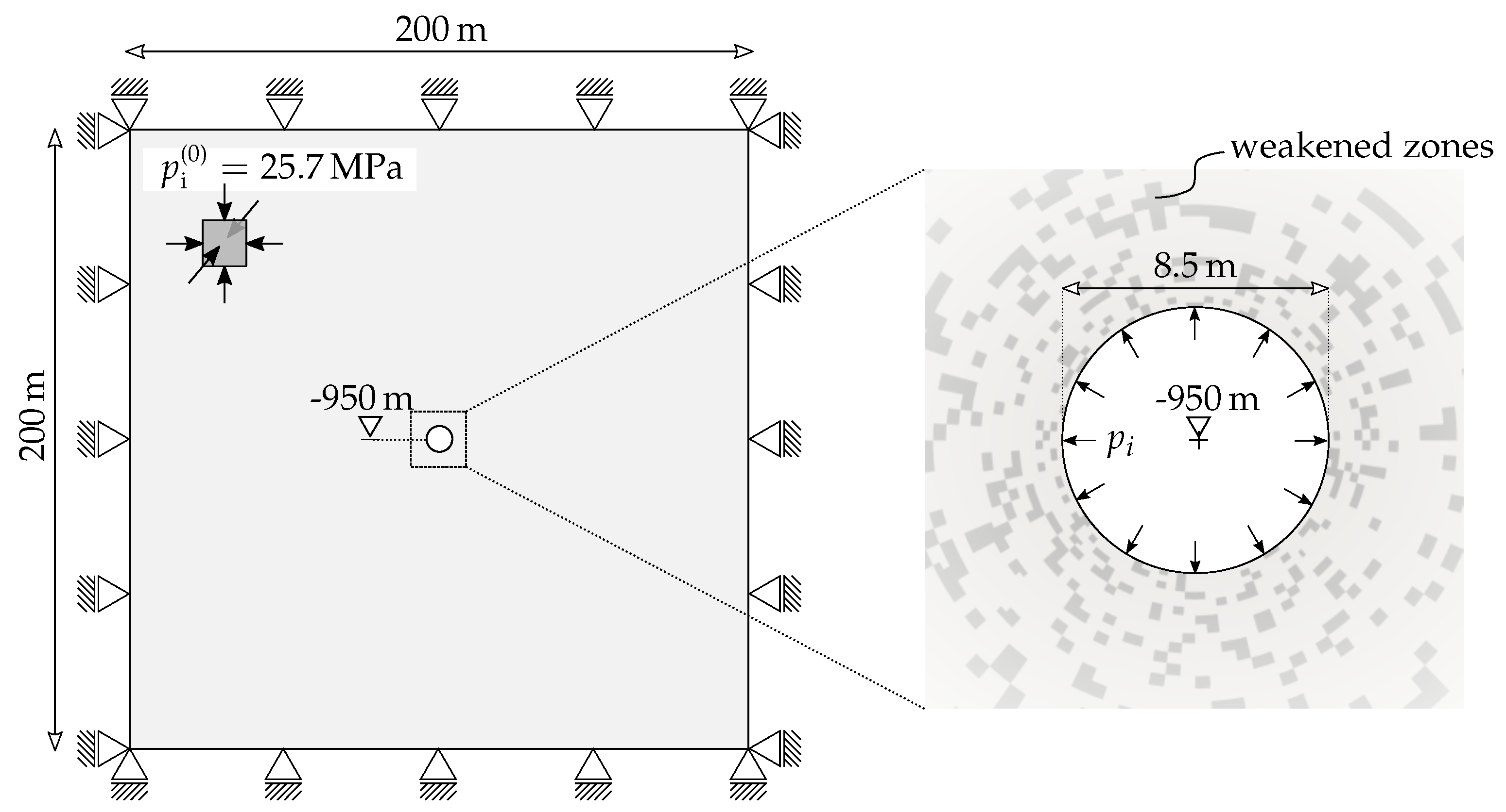
The IBVP of tunnel excavation with its geometry, initial conditions, and boundary conditions is illustrated in Figure 14. Within the discretized domain of rock mass, a hydrostatic geostatic stress state characterized by a pressure of is assumed, corresponding to the overburden at the tunnel axis of 950 m. In the numerical simulations, initial equilibrium is established by applying the geostatic stress state together with the internal pressure acting on the excavation boundary. The excavation procedure is simulated by gradually decreasing the internal pressure to zero. Since the analyzed tunnel section is located in Innsbruck quartz phyllite rock mass, most of the material parameters of Section 4.2 are adopted. The material behavior of rock mass in contrast to intact rock is considered by empirical down-scaling factors based on the geological strength index and the disturbance factor D proposed by Hoek and Brown [27] accounting for the influence of distributed discontinuities. They are taken from the geological survey, reported in [52]. The additional material parameters for Innsbruck quartz phyllite rock mass are , , , , and . To trigger the formation of shear bands in spite of the axisymmetric problem, non-uniformly distributed rock mass properties are employed by introducing zones in which the strength of the rock mass is slightly weakened (indicated in Figure 14). It was verified that these weakened zones do not affect the predicted mechanical response before the onset of strain softening. For investigating the influence of the finite element mesh on the predicted results, three structured meshes with fully integrated and reduced integrated 8-node quadrilateral elements with element sizes of 300 mm (8078 elements), 140 mm (21,414 elements), and 70 mm (55828 elements) in the close vicinity of the tunnel are employed. Both the displacement field and the nonlocal field are approximated by quadratic shape functions.
Upon decreasing the internal pressure, initially the rock mass behavior remains in the linear elastic regime, followed by the formation of plastic zones emerging from the excavation boundary. Once the strength of the rock mass is attained, strain softening is initiated. From the onset of strain softening, the strains are localizing into narrow zones of the rock mass, and, eventually, large displacements accumulate. Finally, at a certain release level of the internal pressure, equilibrium is lost.
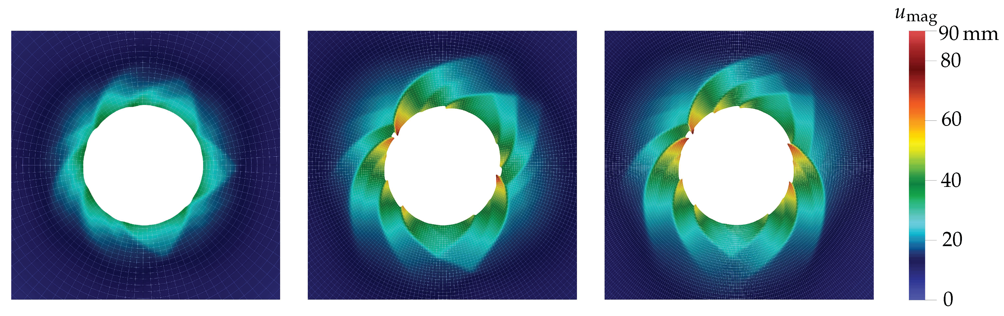
Figure 15 shows the deformed rock mass at the level of 12% of the internal pressure for the three meshes with fully integrated elements. For the medium and the fine mesh, the localization of displacements into narrow zones has already reached a very progressed stage close to failure, and the formation of shear bands is clearly visible. The non-axisymmetric displacement field indicates the transition from an initially quasi-continuous rock mass to quasi-discontinuous rock mass. The latter is characterized by blocks of rock mass moving towards the tunnel center, so potential failure of the tunnel is imminent. Concerning the influence of the finite element discretization, for the medium and the fine mesh, an almost identical displacement field is obtained. Slight differences between those two solutions can be observed only for the upper right quadrant.
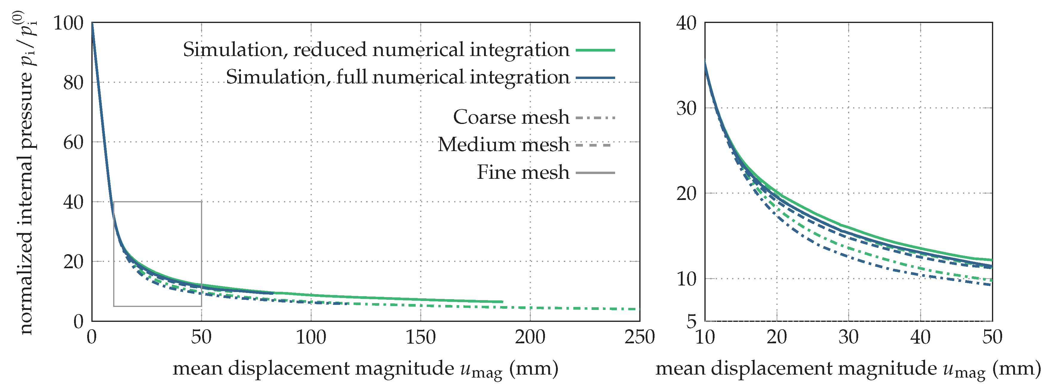
Figure 16 shows the load–displacement curves, i.e., the normalized internal pressure versus the mean displacement magnitude along the excavation boundary computed for each mesh. The load–displacement curves predicted by the three meshes are very close to each other, and, in particular, the results for the medium and the fine mesh are almost identical. The results for the coarse mesh are slightly different due to the already discussed required mesh size for a sufficient resolution of the gradient of the nonlocal field.
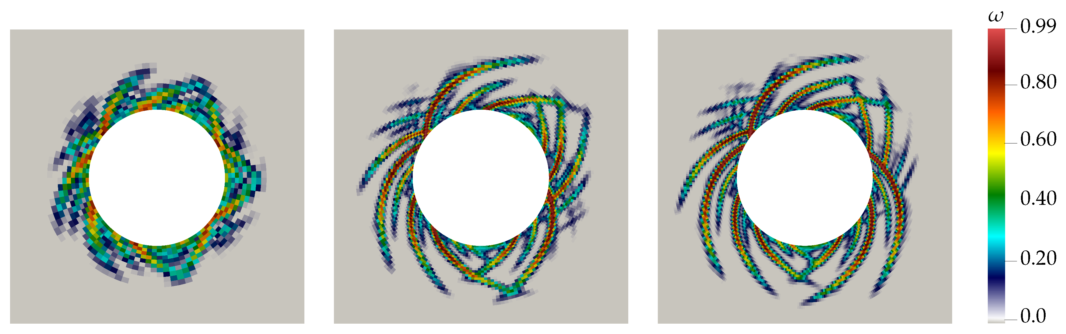
Figure 17 depicts the damaged zones in the rock mass at the level of 12% of the initial internal pressure for the three meshes employing full numerical integration. The highly damaged zones correspond to large shear deformations, which were shown previously in Figure 15. A similar shape of failure zones was obtained by Addis et al. [57] in laboratory tests on a bore hole in weak sandstone. Hence, the potential of the gradient-enhanced approach to predict the onset of failure of a structure was demonstrated in spite of the rather complex failure mode.
5. Conclusions
The present contribution addressed the prediction of complex failure modes in numerical simulations by means of a new implicit gradient-enhanced damage-plasticity model for intact rock and rock mass. It was derived from the damage-plasticity rock model presented by Unteregger et al. [24,25] and extended by adopting the implicit gradient-enhancement proposed in [17]. For the assessment of the model, a comprehensive numerical study was presented. In particular, numerical simulations of wedge splitting tests for evaluating the representation of mode I failure, simulations of triaxial compression and extension tests for evaluating the representation of shear failure under confined stress states, and finally simulations of deep tunneling for examining the prediction of failure mechanisms of a complex structure were performed. From the obtained results of the numerical study, the following conclusions can be drawn:
- In numerical simulations of wedge splitting tests, the formation of a crack propagating from the notch is modeled by the implicit gradient-enhancement in a smeared manner over a width related to the assumed length scale parameter. The capability of the gradient-enhanced damage-plasticity rock model of representing the experimentally observed material behavior was realistically demonstrated.
- Finite element analyses with both structured and unstructured meshes confirmed the regularizing effect of the implicit gradient-enhancement in mode I failure and thus revealed mesh-insensitive results. In particular, it was demonstrated that the crack direction is not biased by the orientation of the finite element mesh.
- Regarding the simulations of triaxial compression tests, a proper representation of shear failure under confined stress states, attaining the compressive meridian of the yield surface, was shown. After attaining peak strength upon initiation of damage, localization into a distinct shear band was observed. Furthermore, reasonable agreement with experimental results, and in particular the experimentally observed increasingly ductile material behavior with increasing confining pressure was obtained.
- The simulations of triaxial extension tests demonstrated that failure under confined stress states attaining the tensile meridian of the yield surface is represented reasonably well, i.e., the localization of damage into a distinct shear band is predicted. In contrast to the triaxial compression tests, a more brittle structural response was observed.
- For both the triaxial compression and extension tests, a mesh study confirmed mesh-insensitive results for shear failure under confined stress states.
- In the numerical simulations of deep tunnel excavation, the rock mass was subjected to softening material behavior due to the excavation procedure, which leads to localization of strains into multiple distinct shear bands. In spite of the complex structural failure mechanism involving the formation of multiple shear bands, mesh insensitive load–displacement curves were obtained. By analyzing the convergence of the damage patterns upon mesh refinement, only slight differences were recognized.
- For the adopted formulation of the implicit gradient-enhanced rock model, the length scale l is assumed as a constant parameter. Thus, a rather broad zone of completely damaged material is predicted by the model. Possible remedies were proposed in the literature, for instance, based on variable length scale parameters [58,59] or the so-called concept of decreasing interactions [45], which is motivated by a physically based micromechanical homogenization theory [60], cf. [46] for a discussion of these approaches. For a more realistic representation of sharp cracks within the present gradient-enhanced rock model, further investigations of these concepts are recommended.
- Regarding the identification of the parameters controlling the gradient-enhanced softening part of the model, i.e., softening modulus , length scale parameter l, and weighting parameter m, an ad hoc approach was employed: While the length scale parameter l was treated as a model parameter conforming to the size of the employed finite element mesh to ensure a sufficient resolution of the nonlocal gradient, was identified by a best fit with experimental results for a chosen l and m. A more systematic approach for identifying these parameters based on experimental results is an open issue. In particular, a scheme to compute based on a prescribed value of l and a typical material parameter, such as the specific mode I fracture energy, is desirable.
Summarizing, it can be concluded that the presented damage-plasticity model is capable of representing a wide range of failure mechanisms in numerical simulations in a realistic and objective manner.
References
Author Contributions
This paper was jointly conceived by M.S., M.N., and G.H.; M.S. and M.N. implemented the numerical framework for the implicit gradient-enhanced model, performed the numerical simulations, and evaluated the results; M.S., M.N., and G.H. wrote the paper.
Funding
This research received no external funding.
Conflicts of Interest
The authors declare no conflict of interest.
References
- Swoboda, G.; Shen, X.P.; Rosas, L. Damage model for jointed rock mass and its application to tunnelling. Comput. Geotech. 1998, 22, 183–203. [Google Scholar] [CrossRef] [Green Version]
- Martin, C.; Kaiser, P.; McCreath, D. Hoek–Brown parameters for predicting the depth of brittle failure around tunnels. Can. Geotech. J. 1999, 36, 136–151. [Google Scholar] [CrossRef]
- Egger, P. Design and construction aspects of deep tunnels (with particular emphasis on strain softening rocks). Tunn. Undergr. Space Technol. 2000, 15, 403–408. [Google Scholar] [CrossRef]
- Jing, L. A review of techniques, advances and outstanding issues in numerical modelling for rock mechanics and rock engineering. Int. J. Rock Mech. Min. Sci. 2003, 40, 283–353. [Google Scholar] [CrossRef]
- Grassl, P.; Jirásek, M. Damage-plastic model for concrete failure. Int. J. Solids Struct. 2006, 43, 7166–7196. [Google Scholar] [CrossRef]
- Bažant, Z.P. Instability, ductility, and size effect in strain-softening concrete. ASCE J. Eng. Mech. Div. 1976, 102, 331–344. [Google Scholar]
- Bažant, Z.P.; Oh, B.H. Crack band theory for fracture of concrete. Mater. Struct. 1983, 16, 155–177. [Google Scholar] [CrossRef] [Green Version]
- Bažant, Z.P.; Jirásek, M. Nonlocal integral formulations of plasticity and damage: Survey of progress. J. Eng. Mech. 2002, 128, 1119–1149. [Google Scholar] [CrossRef]
- De Borst, R. Simulation of strain localization: A reappraisal of the Cosserat continuum. Eng. Comput. 1991, 8, 317–332. [Google Scholar] [CrossRef]
- Needleman, A. Material rate dependence and mesh sensitivity in localization problems. Comput. Methods Appl. Mech. Eng. 1988, 67, 69–85. [Google Scholar] [CrossRef]
- Miehe, C.; Welschinger, F.; Hofacker, M. Thermodynamically consistent phase-field models of fracture: Variational principles and multi-field FE implementations. Int. J. Numer. Methods Eng. 2010, 83, 1273–1311. [Google Scholar] [CrossRef]
- Peerlings, R.H.J.; Geers, M.G.D.; de Borst, R.; Brekelmans, W.A.M. A critical comparison of nonlocal and gradient-enhanced softening continua. Int. J. Solids Struct. 2001, 38, 7723–7746. [Google Scholar] [CrossRef]
- De Borst, R.; Pamin, J. Gradient plasticity in numerical simulation of concrete cracking. Eur. J. Mech. A/Solids 1996, 15, 295–320. [Google Scholar]
- Geers, M.; de Borst, R.; Brekelmans, W.; Peerlings, R. Validation and internal length scale determination for a gradient damage model: Application to short glass-fibre-reinforced polypropylene. Int. J. Solids Struct. 1999, 36, 2557–2583. [Google Scholar] [CrossRef]
- Peerlings, R.H.J.; Massart, T.J.; Geers, M.G.D. A thermodynamically motivated implicit gradient damage framework and its application to brick masonry cracking. Comput. Methods Appl. Mech. Eng. 2004, 193, 3403–3417. [Google Scholar] [CrossRef]
- Pearce, C.J.; Nielsen, C.V.; Bićanić, N. Gradient enhanced thermo-mechanical damage model for concrete at high temperatures including transient thermal creep. Int. J. Numer. Anal. Methods Geomech. 2004, 28, 715–735. [Google Scholar] [CrossRef]
- Poh, L.H.; Swaddiwudhipong, S. Over-nonlocal gradient enhanced plastic-damage model for concrete. Int. J. Solids Struct. 2009, 46, 4369–4378. [Google Scholar]
- Verhoosel, C.V.; Scott, M.A.; Hughes, T.J.R.; de Borst, R. An isogeometric analysis approach to gradient damage models. Int. J. Numer. Methods Eng. 2011, 86, 115–134. [Google Scholar] [CrossRef] [Green Version]
- Zreid, I.; Kaliske, M. Regularization of microplane damage models using an implicit gradient enhancement. Int. J. Solids Struct. 2014, 51, 3480–3489. [Google Scholar] [CrossRef]
- Hosseini, H.; Horák, M.; Zysset, P.; Jirásek, M. An over-nonlocal implicit gradient-enhanced damage-plastic model for trabecular bone under large compressive strains. Int. J. Numer. Methods Biomed. Eng. 2015, 31. [Google Scholar] [CrossRef] [PubMed]
- Zreid, I.; Kaliske, M. A gradient enhanced plasticity–damage microplane model for concrete. Comput. Mech. 2018, 1–19. [Google Scholar] [CrossRef]
- De Borst, R.; Pamin, J.; Geers, M.G. On coupled gradient-dependent plasticity and damage theories with a view to localization analysis. Eur. J. Mech.-A/Solids 1999, 18, 939–962. [Google Scholar] [CrossRef]
- Hoek, E. Brittle fracture of rock. In Rock Mechanics in Engineering Practice; Wiley: London, UK, 1968; Volume 130. [Google Scholar]
- Unteregger, D.; Fuchs, B.; Hofstetter, G. A damage plasticity model for different types of intact rock. Int. J. Rock Mech. Min. Sci. 2015, 80, 402–411. [Google Scholar] [CrossRef]
- Unteregger, D. Advanced Constitutive Modeling of Intact Rock and Rock Mass. Ph.D. Thesis, Innsbruck University, Innsbruck, Austria, 2015. [Google Scholar]
- Hoek, E.; Diederichs, M.S. Empirical estimation of rock mass modulus. Int. J. Rock Mech. Min. Sci. 2006, 43, 203–215. [Google Scholar] [CrossRef]
- Hoek, E.; Brown, E.T. Practical estimates of rock mass strength. Int. J. Rock Mech. Min. Sci. 1997, 34, 1165–1186. [Google Scholar] [CrossRef]
- Hoek, E.; Carranza-Torres, C.; Corkum, B. Hoek–Brown failure criterion—2002 edition. In Proceedings of the 5th North American Rock Mechanics Symposium, 17th Tunnelling Association of Canada, Toronto, ON, Canada, 7–10 July 2002; Hammah, R., Ed.; University of Toronto Press: Toronto, ON, Canada, 2002; pp. 267–273. [Google Scholar]
- Hoek, E.; Brown, E.T. Empirical strength criterion for rock masses. J. Geotech. Geoenviron. Eng. 1980, 106, 1013–1035. [Google Scholar]
- Menétrey, P.; Willam, K.J. Triaxial failure criterion for concrete and its generalization. ACI Struct. J. 1995, 92, 311–318. [Google Scholar]
- Jirásek, M.; Bauer, M. Numerical aspects of the crack band approach. Comput. Struct. 2012, 110, 60–78. [Google Scholar] [CrossRef]
- Peerlings, R.H.J.; de Borst, R.; Brekelmans, W.A.M.; De Vree, J.H.P. Gradient enhanced damage for quasi-brittle materials. Int. J. Numer. Methods Eng. 1996, 39, 68. [Google Scholar] [CrossRef]
- Vermeer, P.A.; Brinkgreve, R.B.J. A new effective non-local strain measure for softening plasticity. In Localisation and Bifurcation Theory for Soils and Rocks; Chambon, R., Desrues, J., Vardoulakis, I., Eds.; CRC Press: Boca Raton, FL, USA, 1994; pp. 89–100. [Google Scholar]
- Di Luzio, G.; Bažant, Z.P. Spectral analysis of localization in nonlocal and over-nonlocal materials with softening plasticity or damage. Int. J. Solids Struct. 2005, 42, 6071–6100. [Google Scholar] [CrossRef]
- Charlebois, M.; Jirásek, M.; Zysset, P.K. A nonlocal constitutive model for trabecular bone softening in compression. Biomech. Model. Mechanobiol. 2010, 9, 597–611. [Google Scholar] [CrossRef] [PubMed]
- Areias, P.; Rabczuk, T.D.; De Sá, J.C. A novel two-stage discrete crack method based on the screened Poisson equation and local mesh refinement. Comput. Mech. 2016, 58, 1003–1018. [Google Scholar] [CrossRef]
- Peerlings, R.H.J.; de Borst, R.; Brekelmans, W.A.M.; Geers, M.G.D. Gradient-enhanced damage modelling of concrete fracture. Mech. Cohesive-Frict. Mater. 1998, 3, 323–342. [Google Scholar] [CrossRef]
- De Borst, R.; Verhoosel, C.V. Gradient damage vs phase-field approaches for fracture: Similarities and differences. Comput. Methods Appl. Mech. Eng. 2016, 312, 78–94. [Google Scholar] [CrossRef] [Green Version]
- Simo, J.C.; Hughes, T.J.R. Computational Inelasticity, Interdisciplinary Applied Mathematics 7; Springer: New York, NY, USA, 1998. [Google Scholar]
- Brühwiler, E.; Saouma, V.E. Fracture testing of rock by the wedge splitting test. In Rock Mechanics Contributions and Challenges, Proceedings of the 31st US Symposium on Rock Mechanics, CO, USA, 18–20 June 1990; Hustrulid, W., Johnson, G., Eds.; CRC Press: Boca Raton, FL, USA, 1990; pp. 287–294. [Google Scholar]
- Blümel, M. Prüfprotokolle Laborversuche Druckversuche Anfahrtstutzen Ahrntal; Technical Report; Institut für Felsmechanik und Tunnelbau TU Graz: Graz, Austria, 2014. [Google Scholar]
- Grassl, P.; Xenos, D.; Jirásek, M.; Horák, M. Evaluation of nonlocal approaches for modelling fracture near nonconvex boundaries. Int. J. Solids Struct. 2014, 51, 3239–3251. [Google Scholar] [CrossRef]
- Pourhosseini, O.; Shabanimashcool, M. Development of an elasto-plastic constitutive model for intact rocks. Int. J. Rock Mech. Min. Sci. 2014, 66, 1–12. [Google Scholar] [CrossRef]
- Jirásek, M.; Grassl, P. Evaluation of directional mesh bias in concrete fracture simulations using continuum damage models. Eng. Fract. Mech. 2008, 75, 1921–1943. [Google Scholar] [CrossRef]
- Poh, L.H.; Sun, G. Localizing gradient damage model with decreasing interactions. Int. J. Numer. Methods Eng. 2017, 110, 503–522. [Google Scholar] [CrossRef]
- Jirásek, M. Regularized continuum damage formulations acting as localization limiters. In Computational Modelling of Concrete Structures, Proceedings of the Conference on Computational Modelling of Concrete and Concrete Structures (EURO-C 2018), Bad Hofgastein, Austria, 26 February–1 March 2018; Meschke, G., Pichler, B., Rots, J.G., Eds.; Taylor & Francis Group: London, UK, 2018; pp. 25–42. [Google Scholar]
- Zervos, A.; Papanastasiou, P.; Cook, J. Elastoplastic finite element analysis of inclined wellbores. In Proceedings of the SPE/ISRM Rock Mechanics in Petroleum Engineering, Trondheim, Norway, 8–10 July 1998; Society of Petroleum Engineers: Richardson, TX, USA, 1998; pp. 1–10. [Google Scholar]
- Fang, Z.; Harrison, J.P. Application of a local degradation model to the analysis of brittle fracture of laboratory scale rock specimens under triaxial conditions. Int. J. Rock Mech. Min. Sci. 2002, 39, 459–476. [Google Scholar] [CrossRef]
- Golshani, A.; Okui, Y.; Oda, M.; Takemura, T. A micromechanical model for brittle failure of rock and its relation to crack growth observed in triaxial compression tests of granite. Mech. Mater. 2006, 38, 287–303. [Google Scholar] [CrossRef]
- De Borst, R. Computation of post-bifurcation and post-failure behavior of strain-softening solids. Comput. Struct. 1987, 25, 211–224. [Google Scholar] [CrossRef] [Green Version]
- Jirásek, M.; Bažant, Z.P. Inelastic Analysis of Structures; John Wiley & Sons, Ltd.: Chichester, UK, 2002. [Google Scholar]
- Schreter, M.; Neuner, M.; Unteregger, D.; Hofstetter, G.; Reinhold, C.; Cordes, T.; Bergmeister, K. Application of a damage plasticity model for rock mass to the numerical simulation of tunneling. In Proceedings of the IV International Conference on Computational Methods in Tunneling and Subsurface Engineering (EURO:TUN 2017), Innsbruck, Austria, 18–20 April 2017; Hofstetter, G., Bergmeister, K., Eberhardsteiner, J., Meschke, G., Schweiger, H.F., Eds.; Innsbruck University: Innsbruck, Austria, 2017; pp. 549–556. [Google Scholar]
- Bobich, J. Experimental Analysis of the Extension to Shear Fracture Transition in Berea Sandstone. Master’s Thesis, Texas A&M University, College Station, TX, USA, 2005. [Google Scholar]
- Neuner, M.; Schreter, M.; Unteregger, D.; Hofstetter, G. Influence of the Constitutive Model for Shotcrete on the Predicted Structural Behavior of the Shotcrete Shell of a Deep Tunnel. Materials 2017, 10, 577. [Google Scholar] [CrossRef] [PubMed]
- Vardoulakis, I.; Sulem, J.; Guenot, A. Borehole instabilities as bifurcation phenomena. Int. J. Rock Mech. Min. Sci. Geomech. Abstr. 1988, 25, 159–170. [Google Scholar] [CrossRef]
- Crook, T.; Willson, S.; Yu, J.G.; Owen, R. Computational modelling of the localized deformation associated with borehole breakout in quasi-brittle materials. J. Pet. Sci. Eng. 2003, 38, 177–186. [Google Scholar] [CrossRef]
- Addis, M.A.; Barton, N.R.; Bandis, S.C.; Henry, J.P. Laboratory studies on the stability of vertical and deviated boreholes. In Proceedings of the SPE Annual Technical Conference and Exhibition, New Orleans, LA, USA, 23–26 September 1990. [Google Scholar]
- Geers, M.G.D. Experimental Analysis and Computational Modeling of Damage and Fracture. Ph.D. Thesis, Einhoven University of Technology, Eindhoven, The Netherlands, 1997. [Google Scholar]
- Geers, M.G.D.; de Borst, R.; Brekelmans, W.A.M.; Peerlings, R.H.J. Strain-based transient-gradient damage model for failure analyses. Comput. Methods Appl. Mech. Eng. 1998, 160, 133–153. [Google Scholar] [CrossRef]
- Sun, G.; Poh, L. Homogenization of intergranular fracture towards a transient gradient damage model. J. Mech. Phys. Solids 2016, 95, 374–392. [Google Scholar] [CrossRef]
Figure 1.
Schematic illustration of two characteristic failure modes (according to [23]): tensile failure (opening mode, left) and shear failure (sliding mode, right).
Figure 1.
Schematic illustration of two characteristic failure modes (according to [23]): tensile failure (opening mode, left) and shear failure (sliding mode, right).

Figure 2.
Geometry and boundary conditions of the numerical model of the specimen for the wedge splitting test.
Figure 2.
Geometry and boundary conditions of the numerical model of the specimen for the wedge splitting test.

Figure 3.
Splitting force vs. crack mouth opening displacement (CMOD) for the wedge splitting test: experimental results (data taken from [40]) and numerical results.
Figure 3.
Splitting force vs. crack mouth opening displacement (CMOD) for the wedge splitting test: experimental results (data taken from [40]) and numerical results.

Figure 4.
Deformed specimen at CMOD = 0.3 mm with a displacement scale factor of 100 for the three structured finite element meshes: coarse—3580 elements (left), medium—6940 elements (center), and fine—15430 elements (right).
Figure 4.
Deformed specimen at CMOD = 0.3 mm with a displacement scale factor of 100 for the three structured finite element meshes: coarse—3580 elements (left), medium—6940 elements (center), and fine—15430 elements (right).

Figure 5.
Distribution of the damage variable at CMOD = 0.3 mm for the three structured finite element meshes: coarse (left), medium (center), and fine (right).
Figure 5.
Distribution of the damage variable at CMOD = 0.3 mm for the three structured finite element meshes: coarse (left), medium (center), and fine (right).

Figure 6.
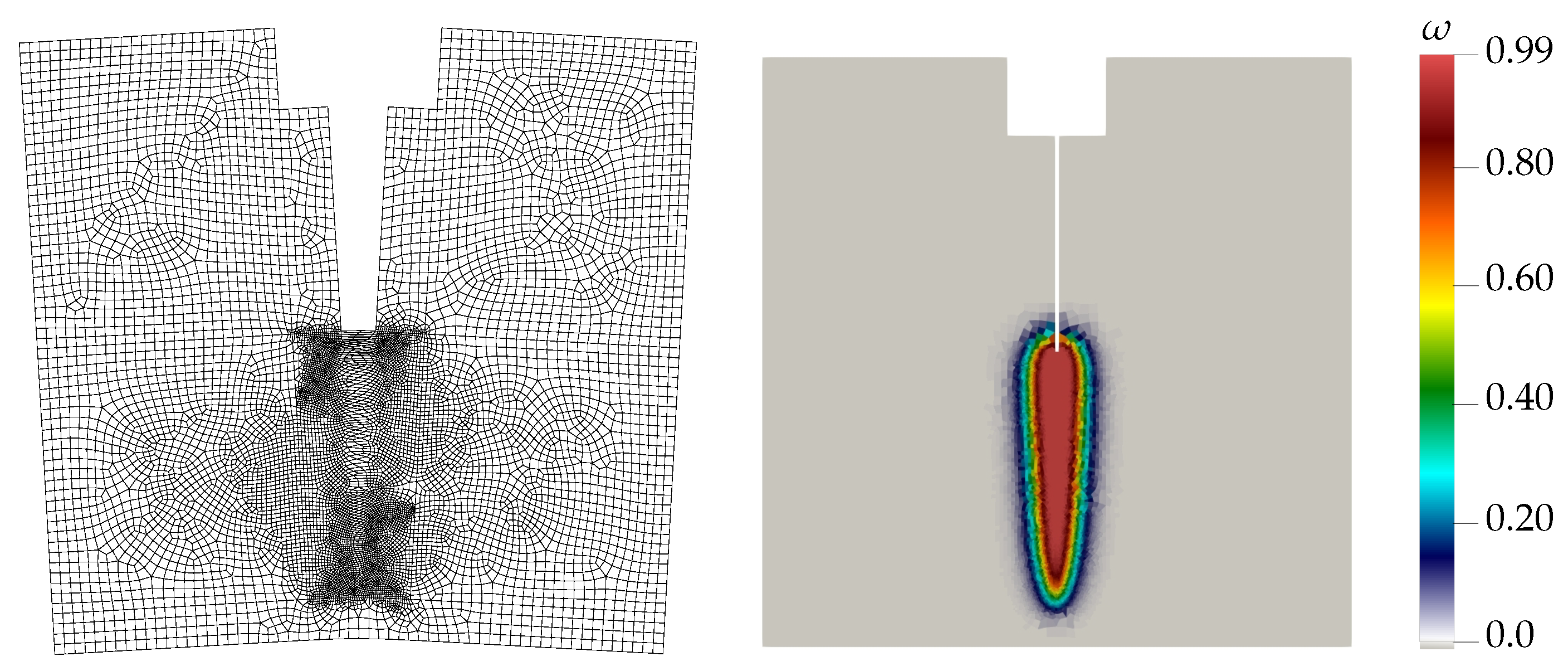
Deformed specimen with a displacement scale factor of 100 (left) and distribution of the damage variable (right) for the unstructured mesh (9504 elements) at a CMOD of 0.3 mm.
Figure 6.
Deformed specimen with a displacement scale factor of 100 (left) and distribution of the damage variable (right) for the unstructured mesh (9504 elements) at a CMOD of 0.3 mm.

Figure 7.
Geometry and boundary conditions of the specimen for the triaxial compression test.

Figure 8.
Load–displacement curves (axial force versus axial displacement) for triaxial compression tests: experimental and numerical results for different levels of confining pressures .
Figure 8.
Load–displacement curves (axial force versus axial displacement) for triaxial compression tests: experimental and numerical results for different levels of confining pressures .

Figure 9.
(a) Distribution of the vertical displacement (scale factor 5) in the final stage of the triaxial compression test with for the three finite element meshes: coarse (left), medium (center), and fine (right). (b) Corresponding deformed rock specimen after a triaxial compression test with , reproduced with permission from M. Bluemel taken from the report [41].

Figure 10.
Distribution of the damage variable in the final stage of the triaxial compression test with for the three finite element meshes: coarse (left), medium (center), and fine (right).
Figure 10.
Distribution of the damage variable in the final stage of the triaxial compression test with for the three finite element meshes: coarse (left), medium (center), and fine (right).

Figure 11.
Triaxial compression tests: distribution of the vertical displacement in the symmetry plane for the four different levels of confining pressure.
Figure 11.
Triaxial compression tests: distribution of the vertical displacement in the symmetry plane for the four different levels of confining pressure.

Figure 12.
Computed load–displacement curves for triaxial extension tests for different levels of confining pressure .
Figure 12.
Computed load–displacement curves for triaxial extension tests for different levels of confining pressure .

Figure 13.
Distribution of the vertical displacement (deformation scale factor 10) at an applied top displacement of 0.1 mm in the triaxial extension test with for the three finite element meshes: coarse (left), medium (center), and fine (right).
Figure 13.
Distribution of the vertical displacement (deformation scale factor 10) at an applied top displacement of 0.1 mm in the triaxial extension test with for the three finite element meshes: coarse (left), medium (center), and fine (right).

Figure 14.
2D initial boundary value problem of deep tunnel excavation: full model (left) and the detail center view (right).
Figure 14.
2D initial boundary value problem of deep tunnel excavation: full model (left) and the detail center view (right).

Figure 15.
Distribution of the magnitude of the displacement vector in the vicinity of the tunnel surface at the level of 12 % of the initial internal pressure with a displacement scale factor of 10 for the three finite element meshes with full numerical integration: coarse (left), medium (center), and fine (right).

Figure 16.
Load–displacement curves: normalized internal pressure versus the mean displacement magnitude at the tunnel surface for the three finite element meshes with full and reduced numerical integration: total view (left), detailed view (right).
Figure 16.
Load–displacement curves: normalized internal pressure versus the mean displacement magnitude at the tunnel surface for the three finite element meshes with full and reduced numerical integration: total view (left), detailed view (right).

Figure 17.
Distribution of the damage variable in the rock mass in the vicinity of the tunnel surface at the level of 12 % of the internal pressure for the three finite element meshes employing full numerical integration: coarse (left), medium (center), and fine (right).
Figure 17.
Distribution of the damage variable in the rock mass in the vicinity of the tunnel surface at the level of 12 % of the internal pressure for the three finite element meshes employing full numerical integration: coarse (left), medium (center), and fine (right).

© 2018 by the authors. Licensee MDPI, Basel, Switzerland. This article is an open access article distributed under the terms and conditions of the Creative Commons Attribution (CC BY) license (http://creativecommons.org/licenses/by/4.0/).
Share and Cite
MDPI and ACS Style
Schreter, M.; Neuner, M.; Hofstetter, G. Evaluation of the Implicit Gradient-Enhanced Regularization of a Damage-Plasticity Rock Model. Appl. Sci. 2018, 8, 1004. https://doi.org/10.3390/app8061004
AMA Style
Schreter M, Neuner M, Hofstetter G. Evaluation of the Implicit Gradient-Enhanced Regularization of a Damage-Plasticity Rock Model. Applied Sciences. 2018; 8(6):1004. https://doi.org/10.3390/app8061004
Chicago/Turabian StyleSchreter, Magdalena, Matthias Neuner, and Günter Hofstetter. 2018. "Evaluation of the Implicit Gradient-Enhanced Regularization of a Damage-Plasticity Rock Model" Applied Sciences 8, no. 6: 1004. https://doi.org/10.3390/app8061004
Note that from the first issue of 2016, this journal uses article numbers instead of page numbers. See further details here.