A Simple High-Order Shear Deformation Triangular Plate Element with Incompatible Polynomial Approximation

Featured Application

Due to the mathematical complexity raised by a high continuity requirement, developing simple/efficient standard finite elements with general polynomial approximations applicable for arbitrary HSDTs seems to be a difficult task at the present theoretical level. In this article, a series of High-order Shear Deformation Triangular Plate Elements (HSDTPEs) are developed using polynomial approximation for the analysis of isotropic thick-thin plates, through-thickness functionally graded plates, and cracked plates. The HSDTPEs have the advantage of simplicity in formulation, are free from shear locking, avoid using a shear correction factor and reduced integration, and provide stable solutions for thick and thin plates. The work can be further applied to plates and shells analysis with arbitrary shapes of elements, as well as more general problems related to the shear deformable effect, such as fracture and functionally graded plates.

Abstract

The High-order Shear Deformation Theories (HSDTs) which can avoid the use of a shear correction factor and better predict the shear behavior of plates have gained extensive recognition and made quite great progress in recent years, but the general requirement of C¹ continuity in approximation fields in HSDTs brings difficulties for the numerical implementation of the standard finite element method which is similar to that of the classic Kirchhoff-Love plate theory. As a strong complement to HSDTs, in this work, a series of simple High-order Shear Deformation Triangular Plate Elements (HSDTPEs) using incompatible polynomial approximation are developed for the analysis of isotropic thick-thin plates, cracked plates, and through-thickness functionally graded plates. The elements employ incompatible polynomials to define the element approximation functions u/v/w, and a fictitious thin layer to enforce the displacement continuity among the adjacent plate elements. The HSDTPEs are free from shear-locking, avoid the use of a shear correction factor, and provide stable solutions for thick and thin plates. A variety of numerical examples are solved to demonstrate the convergence, accuracy, and robustness of the present HSDTPEs.

1. Introduction

The classic Kirchhoff-Love plate theory based on the assumption that a plane section perpendicular to the mid-plane of the plate before deformation remains plane and perpendicular to the deformed mid-plane after deformation is the simplest plate theory in engineering analysis. However, the Kirchhoff-Love plate theory is only applicable for thin plates due to the neglecting of the shear deformation effects. The most well-known and earliest plate theories that take into account the shear deformation effects were proposed by Reissner [1] and Mindlin [2], in which the Mindlin plate theory was based on an assumption of a linear variation of in-plane displacements through the thickness of the plate, referred to as the First-order Shear Deformation Theory (FSDT). The plate elements derived from the FSDT only require C⁰ continuity in approximation fields, have the advantages of physical clarity and simplicity of application [3], and hence were widely accepted and used to model thick-thin plates by scientists and engineers. Unfortunately, the FSDT elements suffer from the shear-locking problem when the thickness to length ration of the plate becomes very small, due to inadequate dependence among transverse deflection and rotations using an ordinary low-order finite element [4]. Quite a large number of techniques have been developed to overcome this problem, such as the assumed shear strain approach, the discrete Kirchhoff/Mindlin representation, the mixed/hybrid formulation, and the reduced/selected integration [5,6,7,8,9,10,11,12,13,14,15]. These formulations are free from shear locking and are applicable to a wide range of practical engineering problems, but in general, it is rather complex and time consuming to include the transverse shear effects for thick plates, which would also lead to complexity and difficulty in the programming. Moreover, the assumption of FSDT causes constant transverse shear strains and stresses across the thickness, which violates the conditions of zero transverse shear stresses on the top and bottom surfaces of plates. A shear correction factor is therefore required to properly compute the transverse shear stiffness. The finding of such a shear correction factor in FSDT is difficult since it depends on geometric parameters, material, loading and boundary conditions, etc. [16].

In recent years, High-order Shear Deformation Theories (HSDTs) have gained extensive recognition and made quite great progress [4,16,17,18,19,20,21,22,23,24,25,26,27,28,29,30,31,32,33,34,35,36,37,38,39,40,41,42,43]. Based on polynomial or non-polynomial transverse shear functions, various HSDTs have been proposed to avoid the use of a shear correction factor, and to better predict the shear behavior of the plate, for instance, the third-order shear deformation theory [17,18], the fifth-order shear deformation theory [19], the exponential shear deformation theory [20], the hyperbolic shear deformation theory [21], and the combined or mixed HSDTs [22,23]. Please see Thai and Kim [16] and Caliri et al. [24] for a comprehensive review of HSDTs. In HSDTs, the bending angles of rotation and shear angles can be treated as independent variables, and the shear-locking problem encountered in FSDT can be well-solved [4]. In [30,31,32,33,34,35,36,37,38,39,40,41,42,43], two well-know HSDTs named as equivalent single layer (ESL) and layer-wise (LW) models are developed to evaluate the effective mechanical behavior of composite structures correctly. The accuracy and reliability of HSDTs have been illustrated by numerous examples in the literature [4,17,25,26,27,28,29,30,31,32,33,34,35,36,37,38,39,40,41,42,43]. However, the general requirement of C¹ continuity in approximation fields in HSDTs brings difficulties for the numerical implementation of the standard Finite Element Method (FEM), which is similar to that of the classic Kirchhoff-Love plate theory. Most examples in the literature are focused on the analytical/numerical solutions of simple Navier-type or Levy-type square plates. The numerical examples reported for the C¹ rectangular finite element using Lagrange interpolation and Hermite interpolation proposed by Reddy [25] and the C⁰ continuous isoparametric Lagrangian finite element with 63 Degrees Of Freedom (DOFs) per element proposed by Gulshan et al. [44] are also limited to the rectangular plate or skew plate. Owing to the striking feature of capturing the high-order continuity well, the Meshless Methods (MM) and IsoGeometric Analysis methods (IGA) appear to be suitable potential methods to construct the numerical formulations for the plate based on HSDTs. The successful implementation of MM [45,46,47,48] and IGA [19,23,49,50,51,52,53,54] in a number of thick-thin plates with arbitrary geometries can be found in the literature.

From the above literature review, it is observed that, due to the mathematical complexity raised by the high continuity requirement, developing simple/efficient standard finite elements with general polynomial approximations applicable for arbitrary HSDTs seems to be a difficult and unreachable task at the present theoretical level. In Cai and Zhu [55], a locking-free MTP9 (Mindlin type Triangular Plate element with nine degrees of freedom) using incompatible polynomial approximation is proposed. It also provides a new way and methodology to develop simple and efficient plate/shell elements based on HSDTs. In this work, with a similar procedure as the MTP9, a series of simple High-order Shear Deformation Triangular Plate Elements (HSDTPEs) using incompatible polynomial approximation are developed for the analysis of isotropic thick-thin plates and through-thickness functionally graded plates. In the HSDTPEs, different orders of general polynomials can be easily employed as element approximation functions, the displacement continuity among the adjacent plate elements can be equivalently enforced by a fictitious thin layer which has a definite physical meaning, and consequently, there are no extra continuity requirements under the theoretical framework of the present HSDTPEs. The HSDTPEs avoid the shear-locking problem and the use of a shear correction factor, and have a good convergence rate and high accuracy for both thick and thin plates. Several representative numerical examples are solved and compared to validate the performance of the present HSDTPEs.

2. Basic Theory of HSDTPEs

2.1. Incompatible Polynomial Approximation over Each Triangular Element

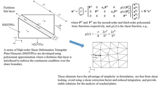
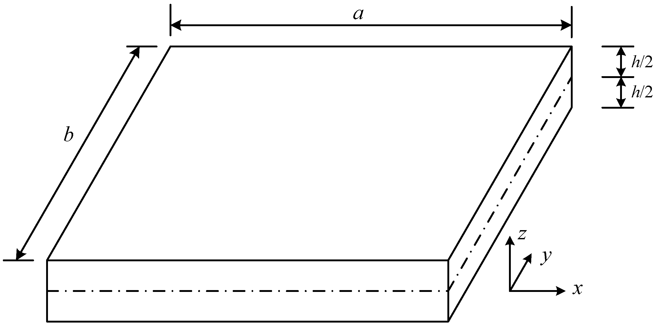
Consider a linear elastic plate with a length $a$, width $b$, and thickness $h$ undergoing infinitesimal deformation, as illustrated in Figure 1. The mid-plane of the plate is divided into arbitrary triangular elements, as shown in Figure 2. The displacement function of the most well-known HSDTs [17] for each triangular element $e_i$ is generally defined by:

$$\{\begin{array}{l}u\left(x,y,z\right)=u_0\left(x,y\right)-z{\theta }_x+g\left(z\right)\left(\frac{\partial w_0}{\partial x}-{\theta }_x\right)\hfill \\ v\left(x,y,z\right)=v_0\left(x,y\right)-z{\theta }_y+g\left(z\right)\left(\frac{\partial w_0}{\partial y}-{\theta }_y\right)\hfill \\ w\left(x,y,z\right)=w_0\left(x,y\right)\hfill \end{array}$$

(1)

where $u_0,v_0$ and $w_0$ are the in-plane and transverse displacements at the mid-plane, respectively; $u={\left[u,v,w\right]}^{\mathrm{T}}$ denotes the displacements of a point $x$ on the plate; ${\theta }_x$ and ${\theta }_y$ are the rotations of the normal to the cross section; $z$ is the coordinate in the transverse direction; and $g\left(z\right)$ describes the distribution of shear effect in the thickness direction. A review of transverse shear functions $g\left(z\right)$ can be found in Nguyen et al. [56]. For isotropic plates with infinitesimal strains, the in-plane displacements $u_0\left(x,y\right)$ and $v_0\left(x,y\right)$ can be neglected because the thickness $h$ is much smaller than the characteristic length $a$ and $b$, and the transverse displacement is much smaller than the thickness $h$, which leads to $u_0\left(x,y\right)\approx 0$ and $v_0\left(x,y\right)\approx 0$ at the mid-plane. The transverse normal displacement $w$ can also be assumed as $w=w\left(x,y,z\right),$ which is not a constant along the $z$ axis, and can be defined by the ESL or LW models [30,31,32,33,34,35,36,37,38,39,40,41,42,43] to capture the effective mechanical behavior along the thickness of composite structures well.

To demonstrate the performance of the present theory for various transverse shear functions, the third-order shear function $g\left(z\right)=-\frac{4z^3}{3h^2}$ [17] and the fifth-order shear function $g\left(z\right)=-\frac{z}{8}-\frac{2z^3}{h^2}+\frac{2z^5}{h^4}$ [19] are used to develop the Third-order Shear Deformation Triangular Plate Element (TrSDTPE) and Fifth-order Shear Deformation Triangular Plate Element (FfSDTPE), respectively. For the special case $g\left(z\right)=0$, Equation (1) is actually the expression of Mindlin plate theory (or FSDT). The corresponding plate element is referred to as FiSDTPE (First-order Shear Deformation Triangular Plate Element) for comparison in the paper.

We assume that:

$$\{\begin{array}{c}{u}_0=P^2{a}^{u_0}\\ v_0=P^2{a}^{v_0}\\ {\theta }_x=P^2{a}^{{\theta }_x}\\ {\theta }_y=P^2{a}^{{\theta }_y}\\ w_0=P^3{a}^w\end{array}$$

(2)

where $a^{u_0}={\left[\begin{array}{cccc}{a}_1& a_2& \cdots & a_6\end{array}\right]}^{\mathrm{T}}$, $a^{v_0}={\left[\begin{array}{cccc}{a}_7& a_8& \cdots & a_{12}\end{array}\right]}^{\mathrm{T}}$, $a^{{\theta }_x}={\left[\begin{array}{cccc}{a}_{13}& a_{14}& \cdots & a_{18}\end{array}\right]}^{\mathrm{T}}$, $a^{{\theta }_y}={\left[\begin{array}{cccc}{a}_{19}& a_{20}& \cdots & a_{24}\end{array}\right]}^{\mathrm{T}}$, $a^w={\left[\begin{array}{cccc}{a}_{25}& a_{26}& \cdots & a_{34}\end{array}\right]}^{\mathrm{T}}$ are the vector of generalized approximation DOFs (degrees of freedom) of the triangular element $e_i$; $P^2$ is the second-order polynomial basis function, and $P^3$ is the third-order polynomial basis function in which:

$$P^2\left(x\right)=\left[\begin{array}{cccccc}1& x_0& y_0& x_0^2& x_0{y}_0& y_0^2\end{array}\right]$$

(3)

$$P^3\left(x\right)=\left[\begin{array}{cccccccccc}1& x_0& y_0& x_0^2& x_0{y}_0& y_0^2& x_0^3& x_0^2{y}_0& y_0^2{x}_0& y_0^3\end{array}\right]$$

(4)

where $x_0=x-x_i$, $y_0=y-y_i$, $\left(x_i,y_i\right)$ are the coordinates of the central point of element $e_i$. It should be noted that only triangular elements, as well as second-order and third-order polynomial functions, are implemented in the paper, but actually, arbitrary shape of elements and arbitrary orders of polynomials can also be easily employed to derive high-order shear deformation plate elements in the present work.

Substituting Equation (2) into Equation (1), the displacement approximation over element $e_i$ can be further expressed as:

$$u^e=\left\{\begin{array}{c}u\\ v\\ w\end{array}\right\}=\left[\begin{array}{ccccc}{P}^2& \mathbf{0}& {\alpha }_z{P}^2& \mathbf{0}& g\left(z\right)P_{,x}^3\\ \mathbf{0}& P^2& \mathbf{0}& {\alpha }_z{P}^2& g\left(z\right)P_{,y}^3\\ \mathbf{0}& \mathbf{0}& \mathbf{0}& \mathbf{0}& P^3\end{array}\right]\left\{\begin{array}{c}{a}^{u_0}\\ a^{v_0}\\ a^{{\theta }_x}\\ a^{{\theta }_y}\\ a^w\end{array}\right\}={\mathbf{N}}^e{\mathbf{a}}^e$$

(5)

where ${\alpha }_z=-z-g\left(z\right)$, $P_{,x}^3=\frac{\partial P^3}{\partial x}$, $P_{,y}^3=\frac{\partial P^3}{\partial y}$,

$${\mathbf{N}}^e=\left\{\begin{array}{c}{\mathbf{N}}^u\\ {\mathbf{N}}^v\\ {\mathbf{N}}^w\end{array}\right\}=\left[\begin{array}{ccccc}{P}^2& \mathbf{0}& {\alpha }_z{P}^2& \mathbf{0}& g\left(z\right)P_{,x}^3\\ \mathbf{0}& P^2& \mathbf{0}& {\alpha }_z{P}^2& g\left(z\right)P_{,y}^3\\ \mathbf{0}& \mathbf{0}& \mathbf{0}& \mathbf{0}& P^3\end{array}\right]$$

(6)

$$a^e={\left[\begin{array}{cccc}{a}_1& a_2& \cdots & a_{34}\end{array}\right]}^{\mathrm{T}}$$

(7)

The strain–displacement relations of the linear elastic problem are given by:

$${\epsilon }_x=\frac{\partial u}{\partial x},{\epsilon }_y=\frac{\partial v}{\partial y},{\epsilon }_z=\frac{\partial w}{\partial z}\approx 0,{\gamma }_{xy}=\frac{\partial u}{\partial y}+\frac{\partial v}{\partial x},{\gamma }_{yz}=\frac{\partial w}{\partial y}+\frac{\partial v}{\partial z},{\gamma }_{xz}=\frac{\partial u}{\partial z}+\frac{\partial w}{\partial x}$$

(8)

Substituting Equation (5) into Equation (8), we have:

$$\mathsf{\epsilon }=\mathbf{L}{u}^e{=\mathbf{LN}}^e{\mathbf{a}}^e{=\mathbf{Ba}}^e$$

(9)

where $\mathsf{\epsilon }={\left[{\epsilon }_x,{\epsilon }_y,{\gamma }_{xy},{\gamma }_{yz},{\gamma }_{xz}\right]}^{\mathrm{T}}$ is the strain vector and $\mathrm{B}$ is the strain matrix, where:

$$\mathbf{B}={\mathbf{LN}}^e$$

(10)

$\mathbf{L}$ is a differential operator where:

$$\mathbf{L}=\left[\begin{array}{ccc}\frac{\partial }{\partial x}& 0& 0\\ 0& \frac{\partial }{\partial y}& 0\\ \frac{\partial }{\partial y}& \frac{\partial }{\partial x}& 0\\ 0& \frac{\partial }{\partial z}& \frac{\partial }{\partial y}\\ \frac{\partial }{\partial z}& 0& \frac{\partial }{\partial x}\end{array}\right]$$

(11)

For an isotropic linear elastic material, the stress–strain relations in element $e_i$ are given by:

$$\sigma ={\mathbf{DBa}}^e$$

(12)

where $\sigma ={\left[{\sigma }_x,{\sigma }_y,{\tau }_{xy},{\tau }_{yz},{\tau }_{xz}\right]}^{\mathrm{T}}$, the transverse stress ${\sigma }_z$ is assumed to be ignored for plate structures, and the elasticity matrix is:

$$D=D_0\left[\begin{array}{ccccc}1& v& 0& 0& 0\\ v& 1& 0& 0& 0\\ 0& 0& \frac{1-v}{2}& 0& 0\\ 0& 0& 0& \frac{1-v}{2k}& 0\\ 0& 0& 0& 0& \frac{1-v}{2k}\end{array}\right]$$

(13)

where $D_0=\frac{E}{1-v^2}$, $E$ is the elastic modulus and $v$ is the Poisson ratio. As mentioned above, a shear correction factor $k$ is required to properly compute the transverse shear stiffness in the FiSDTPE with the assumption of FSDT, which causes constant transverse shear strains and stresses across the thickness and violates the conditions of zero transverse shear stresses on the top and bottom surfaces of plates [16]. Usually, $k$ is taken as $k=1.2$ for the special case of FiSDTPE in Equation (13) according to the principle of the equivalence of strain energy. However, the high-order shear deformation theory gives a parabolic distribution of the transverse stresses/strains directly and avoids the use of a shear correction factor, and thus $k$ is taken as $k=1.0$ in Equation (13) for the rest of the HSDTPEs.

Therefore, the strain energy of element $e_i$ can be derived as:

$${\Pi }^e=\frac{1}{2}{\left({\mathbf{a}}^e\right)}^{\mathrm{T}}{{\displaystyle \int }}_{-h/2}^{h/2}\left({{\displaystyle \iint }}_{∆e_i}{\mathbf{B}}^{\mathrm{T}}\mathbf{DB}dxdy\right)dz{\mathbf{a}}^e$$

(14)

For the plate made of Functionally Graded (FG) materials which is created by mixing two distinct material phases, the composition of the FG materials is in general assumed to be varied continuously from the top to the bottom surface. There are many kinds of FG materials made from all classes of solids. But for the sake of simplicity and convenience, only a ceramic-metal composite is considered and implemented to test the performance of the HSDTPEs in the present study, and the power-law [25,32,45] is used to describe the through-the-thickness distribution of FG materials, which is expressed as:

$$V_c\left(z\right)={\left(\frac{1}{2}+\frac{z}{2}\right)}^n\left(0\le n\le \infty \right)$$

(15)

$$P\left(z\right)=\left(P_c-P_m\right)V_c+P_m$$

(16)

where $n$ is the volume fraction exponent, $V_c$ is the volume fraction of the ceramic, $P_m$ represents the material property of the metal, $P_c$ represents the material property of the ceramic, and $P$ denotes the effective material property. In this work, the Young’s modulus $E$ in Equation (13) varies according to Equation (16) and the Poisson ratio $v$ is assumed to be constant for the analysis of functionally graded plates.

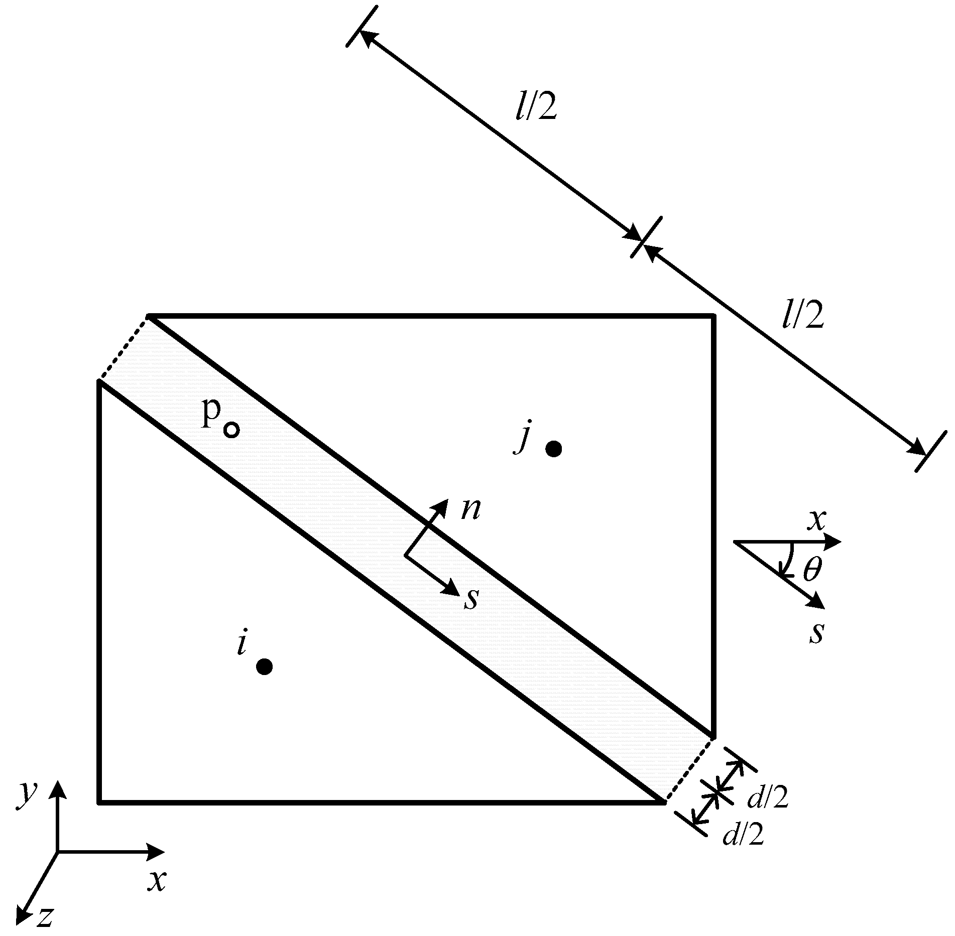
2.2. Fictitious Thin Layer between Adjacent Triangular Elements

According to the definition of the displacement approximation in Equation (5), the deformation along the share boundary of the adjacent elements $e_i$ and $e_j$ is discontinuous, which means that $u^{e_i}\left(x_p,y_p,z_p\right)\ne u^{e_j}\left(x_p,y_p,z_p\right)$ for an arbitrary point $\mathrm{p}$ along the share boundary shown in Figure 2, where point $\mathrm{p}$ has local coordinates $\left(s_p,n_p,z_p\right)$ and global coordinates $\left(x_p,y_p,z_p\right)$. Here, we introduce a fictitious thin layer $e_l$ shown in Figure 3 to enforce the continuous condition over the share boundary of the elements. The geometry dimensions of $e_l$ are the length $l$, width $d$, and height $h$, where $d\ll l$, $d\ll h$, and $h$ is the thickness of the plate in the transverse direction.

Because $d\ll l$ and $d\ll h$, the strain–displacement relations ${\mathsf{\epsilon }}^l={\left[{\gamma }_{ns},{\epsilon }_n,{\gamma }_{nz}\right]}^{\mathrm{T}}$ in thin layer $e_l$ can be simplified as:

$${\gamma }_{ns}=\frac{\partial \overline{u}}{\partial n}\approx \frac{{\overline{u}}^{{\mathrm{p}}^j}-{\overline{u}}^{{\mathrm{p}}^i}}{d},{\epsilon }_n=\frac{\partial \overline{v}}{\partial n}\approx \frac{{\overline{v}}^{{\mathrm{p}}^j}-{\overline{v}}^{{\mathrm{p}}^i}}{d},{\gamma }_{nz}=\frac{\partial \overline{w}}{\partial n}\approx \frac{{\overline{w}}^{{\mathrm{p}}^j}-{\overline{w}}^{{\mathrm{p}}^i}}{d}$$

(17)

where ${\overline{\mathbf{u}}}^{{\mathrm{p}}^i}={\left[{\overline{u}}^{{\mathrm{p}}^i},{\overline{v}}^{{\mathrm{p}}^i},{\overline{w}}^{{\mathrm{p}}^i}\right]}^{\mathrm{T}}$ is the displacement of point $\mathrm{p}$ in the local coordinate $\left(s,n,z\right)$ computed by the approximation of triangular element $e_i$, and ${\overline{\mathbf{u}}}^{{\mathrm{p}}^j}={\left[{\overline{u}}^{{\mathrm{p}}^j},{\overline{v}}^{{\mathrm{p}}^j},{\overline{w}}^{{\mathrm{p}}^j}\right]}^{\mathrm{T}}$ is the displacement of point $\mathrm{p}$ in local coordinate $\left(s,n,z\right)$ computed by the approximation of triangular element $e_j$. ${\overline{\mathbf{u}}}^{{\mathrm{p}}^i}$ and ${\overline{\mathbf{u}}}^{{\mathrm{p}}^j}$ can be calculated using Equation (5).

Substitution of Equation (5) into Equation (17) yields:

$${\mathsf{\epsilon }}^l=\frac{1}{d}{\mathbf{N}}^l{\mathbf{a}}^l$$

(18)

where

$${\mathbf{N}}^l={\mathsf{\lambda }}^l\left[\begin{array}{cc}{\mathbf{-}\mathbf{N}}^{e_i}\left(x_p,y_p,z_p\right)& {\mathbf{N}}^{e_j}\left(x_p,y_p,z_p\right)\end{array}\right]$$

(19)

where ${\mathbf{N}}^{e_i}\left(x_p,y_p,z_p\right)$ is the shape function of point $p$ in triangular element $e_i$ and ${\mathbf{N}}^{e_j}\left(x_p,y_p,z_p\right)$ is the shape function of point $p$ in triangular element $e_j$. ${\mathsf{\lambda }}^l$ is the transformation matrix of point $p$ from the global coordinate $\left(x_p,y_p,z_p\right)$ to the local coordinate $\left(s_p,n_p,z_p\right)$, where:

$${\mathsf{\lambda }}^l=\left[\begin{array}{ccc}\cos \theta & \sin \theta & 0\\ -\sin \theta & \cos \theta & 0\\ 0& 0& 1\end{array}\right]$$

(20)

and

$${\mathbf{a}}^l=\left[\begin{array}{c}{\mathbf{a}}^{e_i}\\ {\mathbf{a}}^{e_j}\end{array}\right]$$

(21)

where ${\mathbf{a}}^{e_i}$ is the DOFs of element $e_i$ and ${\mathbf{a}}^{e_j}$ is the DOFs of element $e_j$.

The stress–strain relations in fictitious thin layer $e_l$ are then given by:

$${\sigma }^l={\mathbf{D}}^l{\mathsf{\epsilon }}^l$$

(22)

where ${\sigma }^l={\left[{\tau }_{ns},{\sigma }_n,{\tau }_{nz}\right]}^{\mathrm{T}}$ and

$${\mathbf{D}}^l=\left[\begin{array}{ccc}{G}_0& 0& 0\\ 0& E_0& 0\\ 0& 0& G_0/k\end{array}\right]$$

(23)

where $G_0=\frac{E}{2\left(1+v\right)}$ and $E_0=\frac{E}{1-v^2}$. Similar to Equation (13), the shear correction factor $k$ is taken as $k=1.2$ for the special case of FiSDTPE, and $k=1.0$ for the rest of the high-order shear deformation plate elements, including the TrSDTPE and FfSDTPE, without the need to use a shear correction factor.

The width $d$ of fictitious thin layer $e_l$ is an important artificial parameter for the present HSDTPEs, but it is easy to select a reasonable $d$ to satisfy $d\ll l$ and $d\ll h$ for simplifying the strain–displacement relations of thin layer $e_l$ in Equation (17). Numerical studies show that the variation of $d$ in a large range has little effect on the accuracy of the calculation results. In this paper, width $d$ is taken as $d=0.0001l$.

Thus, the strain energy of thin layer $e_l$ can be derived as:

$${\Pi }^l=\frac{1}{2d}{\left({\mathbf{a}}^l\right)}^{\mathrm{T}}{{\displaystyle \int }}_{-h/2}^{h/2}\left({{\displaystyle \int }}_{-l/2}^{l/2}{\left({\mathbf{N}}^l\right)}^{\mathrm{T}}{\mathbf{D}}^l{\mathbf{N}}^{l}ds\right)dz{\mathbf{a}}^l$$

(24)

2.3. Imposing Displacement Boundary Condition

As illustrated in Figure 4, along boundary 1–2 of element $e_k$, rotations $\left({\overline{\theta }}_s,{\overline{\theta }}_n\right)$ in the local coordinate $\left(s,n,z\right)$ or the displacements $\left({\overline{u}}_0,{\overline{v}}_0,w_0\right)$ in the local coordinate $\left(s,n,z\right)$ are fixed, where $\left({\overline{u}}_0,{\overline{v}}_0,w_0\right)$ represents the in-plane and transverse displacements at the mid-plane. A fictitious thin layer $e_b$ over boundary 1–2 shown in Figure 4 is also introduced to enforce the displacement boundary condition. We divide the displacement approximation in Equation (5) into two parts to the follow to separately enforce the rotation and mid-plane displacement boundaries.

$${\overline{\mathbf{u}}}^{{\mathrm{p}}_r}\left(s_p,n_p,z_p\right)\approx {\mathsf{\lambda }}^b{\mathbf{N}}^r\left(x_p,y_p,z_p\right){\mathbf{a}}^r$$

(25)

$${\overline{\mathbf{u}}}^{{\mathrm{p}}_t}\left(s_p,n_p,z_p\right)\approx {\mathsf{\lambda }}^b{\mathbf{N}}^t\left(x_p,y_p,z_p\right){\mathbf{a}}^t$$

(26)

where ${\overline{\mathbf{u}}}^{{\mathrm{p}}_r}$ represents the displacement function of point $\mathrm{p}$ for rotations in triangular element $e_k$, ${\overline{\mathbf{u}}}^{{\mathrm{p}}_t}$ represents the displacement function of point $\mathrm{p}$ for mid-plane displacements in triangular element $e_k$, and ${\mathbf{a}}^r$ and ${\mathbf{a}}^t$ are the corresponding DOFs of element $e_k$.

$${\mathbf{N}}^r=\left[\begin{array}{ccccc}\mathbf{0}& \mathbf{0}& {\alpha }_z{P}^2& \mathbf{0}& g\left(z\right)P_{,x}^3\\ \mathbf{0}& \mathbf{0}& \mathbf{0}& {\alpha }_z{P}^2& g\left(z\right)P_{,y}^3\\ \mathbf{0}& \mathbf{0}& \mathbf{0}& \mathbf{0}& 0\end{array}\right]$$

(27)

$${\mathbf{N}}^t=\left[\begin{array}{ccccc}{P}^2& \mathbf{0}& \mathbf{0}& \mathbf{0}& \mathbf{0}\\ \mathbf{0}& P^2& \mathbf{0}& \mathbf{0}& \mathbf{0}\\ \mathbf{0}& \mathbf{0}& \mathbf{0}& \mathbf{0}& P^3\end{array}\right]$$

(28)

where “$\mathbf{0}$” in bold in Equations (27) and (28) represents zero matrix , and ${\mathsf{\lambda }}^b$ is the transformation matrix similar to Equation (20) where

$${\mathsf{\lambda }}^b=\left[\begin{array}{ccc}\cos \omega & \sin \omega & 0\\ -\sin \omega & \cos \omega & 0\\ 0& 0& 1\end{array}\right]$$

(29)

Using the same derivation process as in Equation (24), the strain energy of the thin layer $e_b$ is derived as:

$${\Pi }^b=\frac{1}{2d}{{\displaystyle \int }}_{-h/2}^{h/2}{{\displaystyle \int }}_{-l/2}^{l/2}[{\left(a^r\right)}^T{({\overline{\mathbf{N}}}^r)}^{\mathrm{T}}{D}^r{\overline{\mathbf{N}}}^r{a}^r+{\left(a^t\right)}^T{({\overline{\mathbf{N}}}^t)}^{\mathrm{T}}{D}^t{\overline{\mathbf{N}}}^t{a}^t]dsdz$$

(30)

where ${\mathbf{D}}^b$ is calculated using Equation (23), ${\overline{\mathbf{N}}}^r={\mathsf{\lambda }}^b{\mathbf{N}}^r$, and ${\overline{\mathbf{N}}}^t={\mathsf{\lambda }}^b{\mathbf{N}}^t$.

Please refer to Cai and Zhu [55] for the detailed derivation of the displacement boundary condition fixed at a point or the given displacement boundary condition.

2.4. Load Boundary Condition

A distributed force $f_0={\left[\begin{array}{ccc}0& 0& f_z\end{array}\left(x,y\right)\right]}^{\mathrm{T}}$ along the transverse direction $z$ is applied at element $e_d$, as illustrated in Figure 5. By using Equation (5), the external force potential energy of element $e_d$ is written as:

$${\Pi }^f=-{\left({\mathbf{a}}^{e_d}\right)}^{\mathrm{T}}{{\displaystyle \iint }}_{∆e_d}{\left({\mathbf{N}}^{e_d}\right)}^{\mathrm{T}}{f}_{0}dxdy$$

(31)

where ${\mathbf{N}}^{e_d}$ is the shape function of element $e_d$ calculated by Equation (5), and ${\mathbf{a}}^{e_d}$ is the DOFs of element $e_d$.

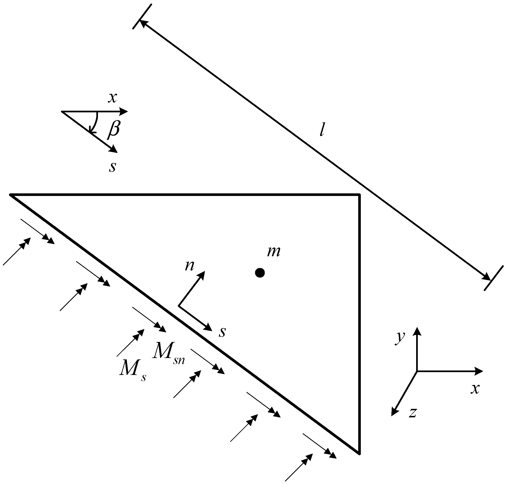
Similarly, a distributed resultant moment $M_0={\left[\begin{array}{ccc}{M}_s& M_{sn}& 0\end{array}\right]}^{\mathrm{T}}$ is applied to the edge of element $e_m$, as illustrated in Figure 6. By using Equation (5), the external force potential energy of element $e_m$ is written as:

$${\Pi }^m=-{\left({\mathbf{a}}^{e_m}\right)}^{\mathrm{T}}{{\displaystyle \int }}_{-l/2}^{l/2}{\left({\mathsf{\lambda }}^m{\tilde{N}}^{e_m}\right)}^{\mathrm{T}}{M}_{0}ds$$

(32)

where ${\mathbf{a}}^{e_m}$ is the DOFs of element $e_m$, and ${\tilde{N}}^{e_m}$ is the shape function of element $e_m$ corresponding to the moment, where:

$${\tilde{N}}^{e_m}=\left[\begin{array}{ccccc}\mathbf{0}& \mathbf{0}& P^2& \mathbf{0}& \mathbf{0}\\ \mathbf{0}& \mathbf{0}& \mathbf{0}& P^2& \mathbf{0}\\ \mathbf{0}& \mathbf{0}& \mathbf{0}& \mathbf{0}& 0\end{array}\right]$$

(33)

and the transformation matrix

$${\mathsf{\lambda }}^m=\left[\begin{array}{ccc}\cos \beta & \sin \beta & 0\\ -\sin \beta & \cos \beta & 0\\ 0& 0& 1\end{array}\right]$$

(34)

2.5. Equilibrium Equation

From Equations (14), (24), (30), (31), and (32), the total potential energy of a plate is obtained as:

$$\Pi =\sum \left({\Pi }^e{+\Pi }^l+{\Pi }^b+{\Pi }^f+{\Pi }^m\right)$$

(35)

The variation of total potential energy $\Pi$ results in the following discrete equation:

$$\frac{\partial \Pi }{\partial \mathbf{a}}=\sum \left({\mathbf{K}}^e{\mathbf{a}}^e+{\mathbf{K}}^l{\mathbf{a}}^l+{\mathbf{K}}^b{\mathbf{a}}^b-{\mathbf{F}}^{ed}-{\mathbf{F}}^{em}\right)=0$$

(36)

where

$${\mathbf{K}}^e={{\displaystyle \int }}_{-h/2}^{h/2}\left({{\displaystyle \iint }}_{∆e_i}{\mathbf{B}}^{\mathrm{T}}\mathbf{DB}dxdy\right)dz$$

(37)

$${\mathbf{K}}^l=\frac{1}{d}{{\displaystyle \int }}_{-h/2}^{h/2}\left({{\displaystyle \int }}_{-l/2}^{l/2}{\left({\mathbf{N}}^l\right)}^{\mathrm{T}}{\mathbf{D}}^l{\mathbf{N}}^{l}ds\right)dz$$

(38)

$${\mathbf{K}}^b=\frac{1}{d}{{\displaystyle \int }}_{-h/2}^{h/2}{{\displaystyle \int }}_{-l/2}^{l/2}\left[{\left({\overline{\mathbf{N}}}^r\right)}^{\mathrm{T}}{\mathbf{D}}^b{\overline{\mathbf{N}}}^r+{\left({\overline{\mathbf{N}}}^t\right)}^{\mathrm{T}}{\mathbf{D}}^b{\overline{\mathbf{N}}}^t\right]dsdz$$

(39)

$${\mathbf{F}}^{ed}={{\displaystyle \iint }}_{∆e_m}{\left({\widehat{N}}^{e_d}\right)}^{\mathrm{T}}{f}_{0}dxdy$$

(40)

$${\mathbf{F}}^{em}={{\displaystyle \int }}_{-l/2}^{l/2}{\left({\mathsf{\lambda }}^m{\tilde{N}}^{e_m}\right)}^{\mathrm{T}}{M}_{0}ds$$

(41)

Assembling the above stiffness matrix and force vector, the equilibrium equation for a plate is then obtained as:

$$\mathbf{K}·\mathbf{U}=\mathbf{F}$$

(42)

where $\mathbf{K}$ is the global stiffness matrix, $\mathbf{F}$ is the force vector, and $\mathbf{U}$ is the vector of DOFs to be solved.

As described in Senjanović et al. [4], the shear-locking problem could be well and naturally solved because the bending angles of rotation and shear angles are treated as independent variables in HSDTs. The regular full integration can be applied to make HSDTPEs valid for the thick-thin plates for the computation of Equation (42), for instance, seven quadrature points for each triangular element [57], four Gauss quadrature points for transverse direction $z$ (where the analytical integration can also be applied for the direction $z$), and four Gauss quadrature points for the local direction $s$ of each fictitious layer are used for the integration of the TrSDTPE using the third-order shear function $g\left(z\right)$ [58,59,60].

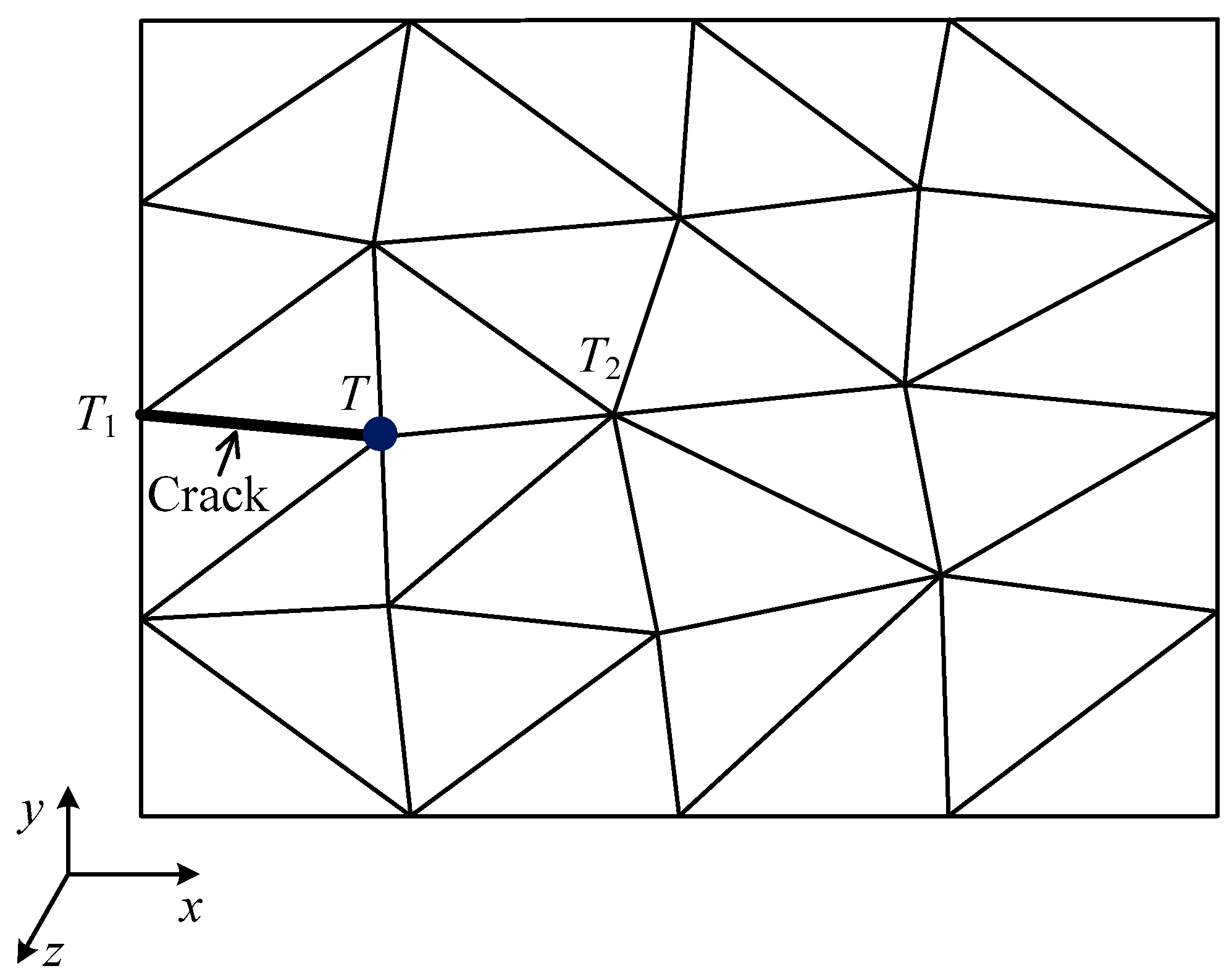
3. Analysis of Cracked Plates

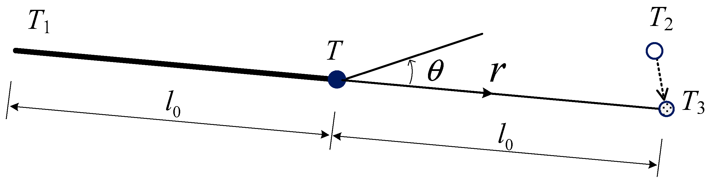
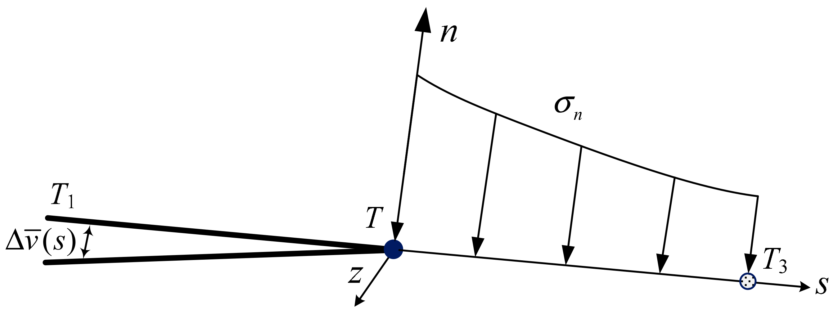
The present HSDTPEs are also applied to the calculation of Stress Intensity Factors (SIFs) of cracked thick-thin plates. As illustrated in Figure 7, the mid plane of a cracked plate is taken as the x-y plane and is divided into arbitrary triangular elements. Accurate computation of SIFs remains challenging in the field of fracture mechanics. For plates loaded by a combination of bending and tension, the SIFs can also be computed by the Virtual Crack Closure Technique (VCCT) [61,62,63], the path-independent J-integral technique or interaction integral [64,65], and the stiffness derivative method [66]. In this paper, the Virtual Crack Closure Technique (VCCT) [61,62,63] is employed to calculate the SIFs of the cracked plate. For the convenience of implementing the VCCT, point $T_2$ shown in Figure 7 and Figure 8 is temporarily moved to $T_3$ along the extended line direction of $T_1-T$. In the local coordinates $\left(s,n,z\right)$ shown in Figure 9, the relative displacements $\left[∆\overline{u}\left(s,z\right),∆\overline{v}\left(s,z\right),∆\overline{w}\left(s,z\right)\right]$ of $T_1-T$ and the stresses $\left[{\tau }_{ns}\left(s,z\right),{\sigma }_n\left(s,z\right),{\tau }_{nz}\left(s,z\right)\right]$ of $T-T_1$ can be easily calculated using Equations (18) and (22) for the fictitious thin layer $e_l$. For example, assuming that the $T_1-T$ is simulated by a fictitious thin layer with width $d$ shown in Figure 3, the relative displacements can be evaluated by $∆\overline{u}\left(s,z\right)={\gamma }_{ns}d$, $∆\overline{v}\left(s,z\right)={\epsilon }_{n}d$ and $∆\overline{w}\left(s,z\right)={\gamma }_{nz}d$. Then, the energy release rate at crack tip $T$ is obtained by the VCCT as:

$$\{\begin{array}{l}{G}_{\mathrm{I}}\cong \frac{1}{2h{r}_0}{{\displaystyle \int }}_{-h/2}^{h/2}{{\displaystyle \int }}_0^{r_0}{\sigma }_n\left(s,z\right)∆\overline{v}\left(s-r_0,z\right)\mathrm{ds}\mathrm{dz}\\ G_{\mathrm{II}}\cong \frac{1}{2h{r}_0}{{\displaystyle \int }}_{-h/2}^{h/2}{{\displaystyle \int }}_0^{r_0}{\tau }_{ns}\left(s,z\right)∆\overline{u}\left(s-r_0,z\right)\mathrm{ds}\mathrm{dz}\\ G_{\mathrm{III}}\cong \frac{1}{2h{r}_0}{{\displaystyle \int }}_{-h/2}^{h/2}{{\displaystyle \int }}_0^{r_0}{\tau }_{nz}\left(s,z\right)∆\overline{w}\left(s-r_0,z\right)\mathrm{ds}\mathrm{dz}\end{array}$$

(43)

where $G_{\mathrm{I}}$ is the energy release rate of crack mode $\mathrm{I}$, $G_{\mathrm{II}}$ is that of crack mode $\mathrm{II}$, and $G_{\mathrm{III}}$ is that of crack mode $\mathrm{III}$. Then, the SIFs of the crack tip can be computed by means of the relations between the energy release rate and SIFs for the plate theory, for instance, $K_1=\sqrt{3E{G}_{\mathrm{I}}}$ [63].

4. Numerical Examples

4.1. Simply Supported Square Plate Subjected to Uniform Load

A simply supported square plate subjected to a uniform load $q$ is tested to show the reliability and convergence of the present elements. The side length of the plate is $L$, and the thickness of the plate is $h$. A quarter of the plate is modeled as a result of symmetry, as illustrated in Figure 10. For the isotropic plates, the in-plane displacements $\left(u_0,v_0\right)$ and their DOFs in Equations (1), (2), and (5) are neglected in the following analyses. The displacement boundary conditions of the present theory along the simply supported edges in local coordinates are ${\overline{\theta }}_s=0$ and $w=0$. The $n\times n$ regular mesh and irregular mesh illustrated in Figure 11 and Figure 12 are employed for convergence studies.

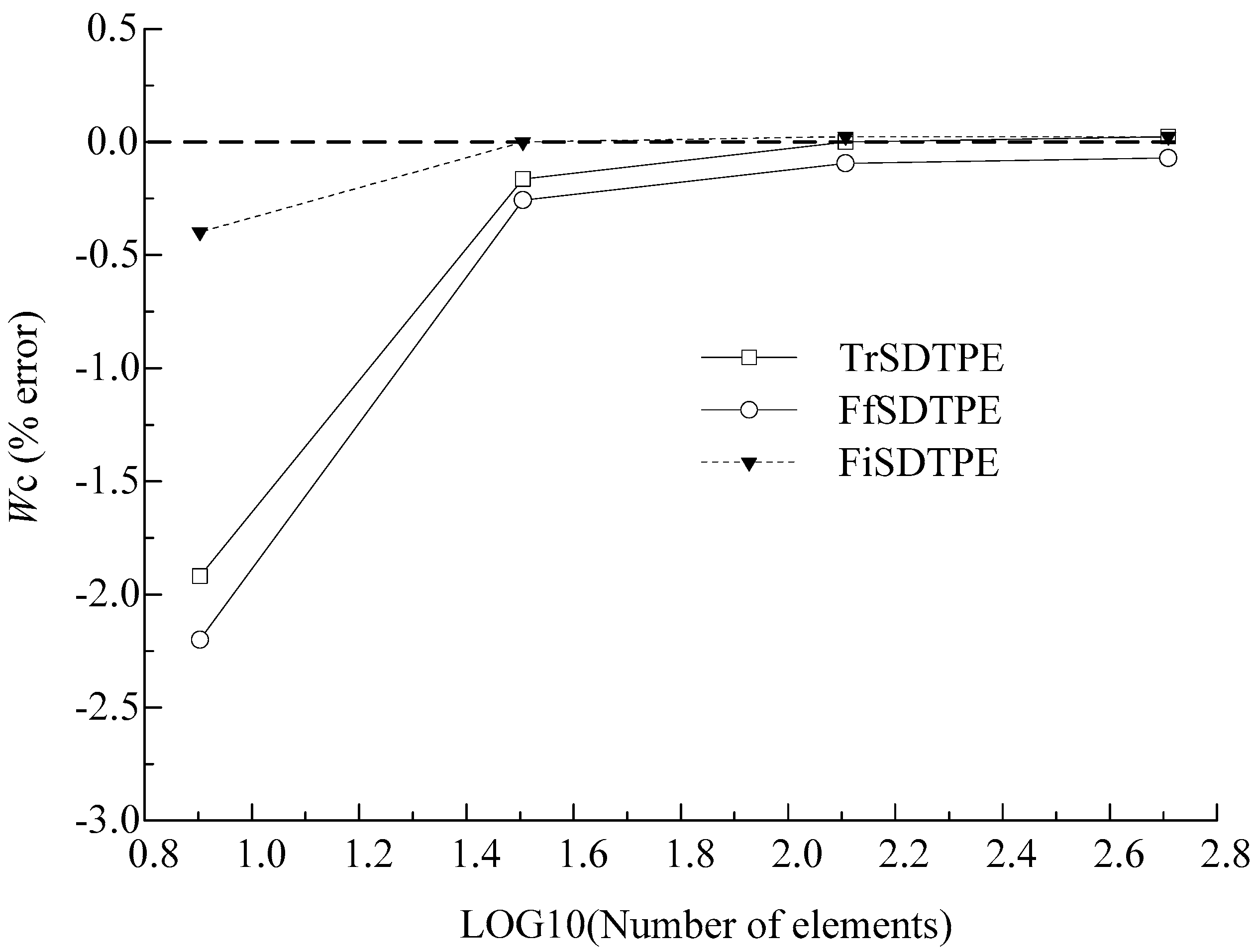
The elements DST-BL (Discrete Mindlin triangular plate element) [7] and RDKTM (Re-constituting discrete Kirchhoff triangular plate element) [14] have been selected for comparison with the present elements based on HSDTs. The reference solutions in the following

Table 1. Normalized deflection for the simply supported square plate.

h/L	0.001	0.01	0.10	0.15	0.20	0.25	0.30
TrSDTPE (4 × 4)	0.4027	0.4050	0.4266	0.4529	0.4897	0.5367	0.5941
TrSDTPE (8 × 8)	0.4058	0.4064	0.4273	0.4536	0.4903	0.5375	0.5949
TrSDTPE (16 × 16)	0.4063	0.4065	0.4274	0.4536	0.4904	0.5375	0.5950
TrSDTPE (Figure 12)	0.4063	0.4066	0.4274	0.4537	0.4904	0.5375	0.5950
FfSDTPE (16 × 16)	0.4063	0.4065	0.427	0.4528	0.4888	0.5350	0.5911
FiSDTPE (16 × 16)	0.4063	0.4065	0.4274	0.4537	0.4905	0.5379	0.5958
DST-BL (16 × 16)	0.4057	0.4059	0.4267	0.4529	0.4896	0.5367	0.5944
RDKTM (16 × 16)	0.4057	0.4059	0.4270	0.4532	0.4899	0.5371	0.5847
Ref. [67]	0.4064	0.4064	0.4273	0.4536	0.4906	0.5379	0.5956

,

Table 2. Normalized bending moment for the simply supported square plate.

h/L	0.001	0.01	0.10	0.15	0.20	0.25	0.30
TrSDTPE (4 × 4)	0.4266	0.4531	0.4741	0.4771	0.4785	0.4791	0.4794
TrSDTPE (8 × 8)	0.4633	0.4734	0.4786	0.4789	0.4791	0.4791	0.4791
TrSDTPE(16 × 16)	0.4759	0.4778	0.4788	0.4789	0.4789	0.4789	0.4789
TrSDTPE (Figure 12)	0.4807	0.4806	0.4807	0.4807	0.4807	0.4807	0.4807
FfSDTPE (16 × 16)	0.4757	0.4775	0.4788	0.4788	0.4788	0.4788	0.4788
FiSDTPE (16 × 16)	0.4762	0.4789	0.479	0.4790	0.4790	0.4790	0.4790
DST-BL (16 × 16)	0.4792	0.4788	0.4773	0.4770	0.4768	0.4767	0.4767
RDKTM (16 × 16)	0.4792	0.4790	0.4789	0.4790	0. 4790	0.4790	0.4790
Ref. [67]	0.4789

,

Table 3. Convergence of normalized deflection with different width-to-length ratios.

$\mathit{d}/\mathit{l}$	0.1	0.01	0.001	0.0001	0.00001	0.000001	0.0000001
TrSDTPE	0.5235	0.4371	0.4283	0.4274	0.4273	0.4273	0.4273
FfSDTPE	0.5229	0.4367	0.4279	0.4270	0.4269	0.4269	0.4269
FiSDTPE	0.5247	0.4372	0.4283	0.4274	0.4273	0.4273	0.4273
Ref. [67]	0.4273

,

Table 4. Normalized deflection for the clamped square plate.

h/L	0.001	0.01	0.10	0.15	0.20	0.25	0.30
TrSDTPE (4 × 4)	0.1171	0.1241	0.1459	0.1708	0.2044	0.2463	0.2962
TrSDTPE (8 × 8)	0.1255	0.1266	0.1491	0.1757	0.2112	0.2553	0.3077
TrSDTPE (16 × 16)	0.1265	0.1268	0.1497	0.1766	0.2124	0.2569	0.3097
TrSDTPE (Figure 12)	0.1266	0.1268	0.1496	0.1764	0.2122	0.2567	0.3095
FfSDTPE (16 × 16)	0.1265	0.1268	0.1491	0.1750	0.2093	0.2516	0.3013
FiSDTPE (16 × 16)	0.1265	0.1268	0.1505	0.1788	0.2173	0.2659	0.3247
DST-BL (16 × 16)	0.1265	0.1267	0.1488	0.1756	0.2127	0.2601	0.3179
RDKTM (16 × 16)	0.1265	0.1267	0.1502	0.1784	0.2167	0.2650	0.3236
Ref. [67]	0.1265	0.1265	0.1499	0.1798	0.2167	0.2675	0.3227

,

Table 5. Comparisons of the normalized deflections with 3D FEM solutions for thick plates.

h/L	0.20	0.25	0.30
TrSDTPE (16 × 16)	0.2124(0.19%)	0.2569(−0.42%)	0.3097(−1.02%)
FfSDTPE (16 × 16)	0.2093(−1.27%)	0.2516(−2.48%)	0.3013(−3.71%)
FiSDTPE (16 × 16)	0.2173(2.50%)	0.2659(3.06%)	0.3247(3.77%)
DST-BL (16 × 16)	0.2127(0.33%)	0.2601(0.81%)	0.3179(1.60%)
RDKTM (16 × 16)	0.2167(2.22%)	0.2650(2.71%)	0.3236(3.42%)
3D FEM	0.2120	0.2580	0.3129

Note: Value in parentheses is the relative error with respect to 3D FEM.

and

Table 6. Normalized deflection for the clamped circular plate.

h/L	0.001	0.01	0.10	0.15	0.20	0.25	0.30
TrSDTPE (32)	1.3964	1.5225	1.6029	1.6846	1.798	1.9428	2.1187
TrSDTPE (128)	1.5441	1.5572	1.6262	1.7119	1.8312	1.9835	2.1682
TrSDTPE (512)	1.5607	1.5622	1.6316	1.7186	1.8394	1.9935	2.1801
TrSDTPE (2048)	1.5626	1.5632	1.6330	1.7203	1.8414	1.9957	2.1825
FfSDTPE (2048)	1.5620	1.5632	1.6315	1.7166	1.8343	1.9836	2.1637
FiSDTPE (2048)	1.5623	1.5633	1.6340	1.7233	1.8483	2.0090	2.2054
DST-BL (2048)	1.5634	1.5642	1.6452	1.7385	1.8665	2.0293	2.2273
RDKTM (2048)	1.5634	1.5640	1.6346	1.7239	1.8490	2.0098	2.2063
Ref. [67]	1.5625	1.5632	1.6339	1.7232	1.8482	2.0089	2.2054

are taken from Long et al. [67], which are also labeled as analytical solutions in [67]. Table 1 lists the normalized defection $W_0=W_c/\frac{q{L}^4}{100D_b}$ of the simply supported square plate, where $W_c$ is the central deflection of the plate and $D_b=\frac{E{h}^3}{12\left(1-v^2\right)}$. Table 2 reports the normalized bending moment $M_0=M_c/\frac{q{L}^2}{10}$ of the simply supported square plate, where $M_c$ is the central bending moment of the plate. The convergence of the deflection for the simply supported square plate using different elements when the aspect ratio h/L = 0.1 is shown in Figure 13. It is observed that all the present TrSDTPE, FfSDTPE, and FiSDTPE shows a good convergence rate and high accuracy, and avoids the shear-locking problem. The results also indicate that the present elements are insensitive to element distortions of the irregular mesh shown in Figure 12.

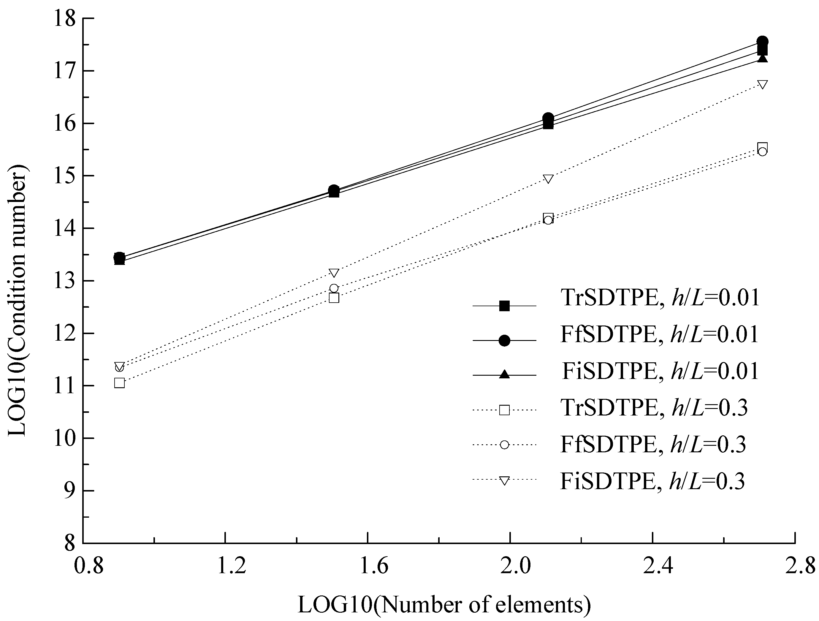
The width-to-length ratio $d/l$ of the fictitious thin layer $e_l$ plays an important role in the present formulations. Table 3 reports the effect of the ratio $d/l$ on the normalized defection $W_0$ for the simply supported square plate, where $16\times 16$ regular mesh and an aspect ratio of $h/L=0.1$ are employed. The results in Table 3 indicate that the artificial parameter $d/l$ has little effect on the solution accuracy when $d/l\le 0.001$, and it is easy to select a reasonable $d$ in the current formulation. In this work, width $d$ is taken as $d=0.0001l$. The condition numbers of the global stiffness matrices of the simply supported square plate using the present elements are also computed and reported in Figure 14. As seen, the variation of the condition number in Figure 14 reflects that the present elements show a good conditioning and stability in the case of mesh refinement.

4.2. Clamped Square Plate Subjected to Uniform Load

A clamped square plate subjected to a uniformly distributed load $q$ is further investigated to test the performance of the present elements for clamp boundary conditions. The geometry and material parameters of the clamped plate are the same as those of the above simply supported plate. The displacement boundary conditions of the present theory along the clamped edges in Figure 10 in local coordinates are ${\overline{\theta }}_s=0,{\overline{\theta }}_n=0$ and $w=0$.

The results for the normalized central deflection $W_0$ of the clamped square plate are compared in Table 4. It is seen that, for the plate with the clamped boundary conditions, the predictions of FiSDTPE, DST-BL, and RDKTM based on FSDT agree well with the reference solutions [67] for plates, but the TrSDTPE and FfSDTPE based on HSDTs seem to underestimate the deflections compared with the reference solutions [67] for thick plates of $h/L\ge 0.2$. To further illustrate the accuracy of the present shear elements, the comparisons of the predictions by different elements and the solutions by 3D elasticity FEM software ANSYS using 20-nodes hexahedron isoparametric element and an element side length of 0.05 are listed in Table 5. By taking the 3D FEM solutions as the benchmark, Table 5 indicates that the present TrSDTPE and FfSDTPE show better solution accuracy than the elements DST-BL, RDKTM, and FiSDTPE based on FSDT for the plates involving clamp boundaries. Moreover, the TrSDTPE with a third-order shear function $g\left(z\right)$ shows the best solution accuracy among all the elements for the clamped plate.

The DOFs of the different methods employed in Table 5 are compared by taking the case of $h/L=0.3$ for the clamped plate. Assuming that a $16\times 16$ regular mesh is employed for the plate element discretization and a $16\times 16\times 9$ regular mesh for the 20-nodes hexahedron 3D element discretization, we can see that the total DOFs of the DST-BL/RDKTM element, HSDTs, and 3D 20-nodes hexahedron element are 867, 17408, and 41337, respectively. It is seen that the total DOFs and the efficiency of HSDTs are between the DST-BL/RDKTM and the 3D FEM. Although the number of DOFs only decreases to 42% of the 3D FEM method, the present 2D HSDTs have the advantage of simplicity and flexibility in the mesh generation compared with 3D FEM for the plates with different thicknesses. Compared with other 2D plate elements such as DST-BL and RDKTM, the computational DOFs of the present 2D HSDTs seem to be relatively higher, but the formulation and the numerical implementation of the high-order shear deformation theory in the present HSDTs are much simpler than those of the DST-BL/RDKTM. From the point of view of the 2D analysis, the total computational cost of the present elements is bearable and worthy in terms of its advantages in formulation and implementation. HSDTs which have almost the same computational efficiency of DST-BL/RDKTM could also be constructed using the reduced integral method similar to our previous work [55], but the present HSDTs avoiding the reduced integration by paying a certain computational cost are more practicable in engineering analysis.

4.3. Clamped Circular Plate Subjected to Uniform Load

A clamped circular plate subjected to a uniformly distributed load $q$ is taken into consideration in this section. The thickness of the plate is $h$. The radius of the plate is $r=100$. A quarter of the plate with symmetry conditions on axes $x$ and $y$ is modeled in Figure 15. The displacement boundary conditions of the present theory along the clamped edges in local coordinates are ${\overline{\theta }}_s=0,{\overline{\theta }}_n=0$, and $w=0$. Divisions of 32, 128, 512, and 2048 triangular elements are employed for the convergence studies. Typical meshes of 512 and 2048 triangular elements for the circular plate are shown in Figure 16. The results for normalized deflection $W_0=W_c/\frac{q{r}^4}{100D_b}$ of the clamped circular plate are listed in Table 6, where $W_c$ is the central deflection of the circular plate. Again, an excellent agreement between the present solutions and the reference solutions is observed for this problem.

4.4. Rectangular Plate Involving a Center Crack

Consider a rectangular plate involving a center crack as shown in Figure 17. The material properties are $E=1.0\times {10}^6\mathrm{Pa}$ and $v=0.3$. The width and length are $2b=1\mathrm{m}$ and $2c=2\mathrm{m}$, respectively. The crack length is $2a$ and the plate thickness is $h$. Divisions of 2728 and 7338 triangular elements are employed for the calculation of SIFs of the center crack plate. The displacement and moment boundary conditions are also illustrated in Figure 17. The numerical results obtained by TrSDTPE, FfSDTPE, and FiSDTPE for different $a/h$ values are reported in

Table 7. Normalized SIFs $F_1$ for the center cracked plate.

a/h	0.8 (0.2/0.25)	1.0 (0.25/0.25)	4.0 (0.2/0.05)	5.0 (0.25/0.05)
TrSDTPE (2728)	0.8577	0.8981	0.7235	0.7602
TrSDTPE (7338)	0.8589	0.9005	0.7243	0.7622
FfSDTPE (7338)	0.8548	0.8968	0.7224	0.7610
FiSDTPE (7338)	0.8627	0.9036	0.7266	0.7633
Tanaka [68]	0.8683	0.9096	0.7287	0.7663
Boduroglu [69]	0.8694	0.9094	0.7347	0.7702

, along with the reference solutions by Tanaka et al. [68] and Boduroglu et al. [69] based on FSDT for comparison. In Tanaka et al. [68], a cracked plate is analyzed by employing the mesh-free reproducing kernel approximation formulated by Mindlin-Reissner plate theory, and the moment intensity factor is evaluated by the J-integral with the aid of nodal integration. In Boduroglu et al. [69], the crack problem is solved by the dual boundary element method based on Reissner plate formulation, and the stress resultant intensity factor is calculated by employing the J-integral techniques. The SIFs in Table 7 are normalized by $F_1=\frac{h^2{K}_1}{6M\sqrt{\pi a}}$. It is observed that the present elements show a high solution accuracy for the calculation of the SIFs.

4.5. Symmetric Edge Cracks in a Rectangular Plate

As illustrated in Figure 18, a rectangular plate with symmetric double edge cracks is analyzed in this example. The geometry dimensions, material properties, and boundary conditions are the same as those of the center cracked problem described in Section 4.4. The crack length is $a$ and the plate thickness is $h$. Division of 2728 triangular elements shown in Figure 17 is also employed for this analysis. The normalized SIFs obtained by the present elements for different values of $d/b$ and $b/h$ are presented in

Table 8. Normalized SIFs $F_1$ for the symmetric edge cracks problem ($b/h=2.0$).

d/b	0.2	0.3	0.4	0.5	0.6
TrSDTPE	1.3429	1.1024	0.9739	0.9016	0.8601
FfSDTPE	1.3353	1.0971	0.9697	0.8990	0.8568
FiSDTPE	1.3502	1.1070	0.9776	0.9028	0.8629
Tanaka [68]	1.3719	1.1201	0.9886	0.9110	0.8706
Boduroglu [69]	1.3689	1.1174	0.9844	0.9086	0.8673

and

Table 9. Normalized SIFs $F_1$ for the symmetric edge cracks problem ($b/h=10.0$).

d/b	0.2	0.3	0.4	0.5	0.6
TrSDTPE	1.0966	0.9156	0.8201	0.7687	0.7317
FfSDTPE	1.0941	0.9140	0.8187	0.7690	0.7306
FiSDTPE	1.0995	0.9173	0.8218	0.7656	0.7328
Tanaka [68]	1.1144	0.9225	0.8246	0.7697	0.7377
Boduroglu [69]	1.1140	0.9250	0.8268	0.7692	0.7351

, along with reference solutions [68,69]. The numerical methods and plate theories for solving the problem are the same as the above rectangular plate problem involving a center crack. As expected, the present results are in good agreement with the reference solutions.

4.6. Simply Supported FG Plate

In this section, a simply supported FG plate subjected to a uniformly distributed load $q$ is analyzed and compared. The FG plate is comprised of aluminum ($E_m=70 GPa,v_m=0.3$) and ceramic ($E_c=151GPa,v_c=0.3$). The side length of the plate is $L=1m$, and the thickness of the plate is $h$. A quarter of the FG plate is modeled as a result of symmetry, as shown in Figure 19. The displacement boundary conditions for the symmetric and simply supported sides in local coordinates are also illustrated in Figure 19. The $16\times 16$ regular mesh similar to Section 4.1 is employed for computation.

Table 10. Normalized deflection for the FG plate (h/L = 0.2).

Exponent n	TrSDTPE	FfSDTPE	FiSDTPE	Ferreira et al. [45]	Talha & Singh [70]
0.0 (ceramic)	0.0248	0.0247	0.0248	0.0248	0.0250
0.5	0.0314	0.0313	0.0315	0.0314	0.0319
1.0	0.0352	0.0351	0.0353	0.0352	0.0358
2.0	0.0389	0.0388	0.0387	0.0388	0.0393
Metal	0.0535	0.0534	0.0536	0.0534	0.0541

and

Table 11. Normalized deflection for the FG plate (h/L = 0.05).

Exponent n	TrSDTPE	FfSDTPE	FiSDTPE	Ferreira et al. [45]
0.0 (ceramic)	0.0208	0.0208	0.0208	0.0208
0.5	0.0266	0.0266	0.0266	0.0265
1.0	0.0298	0.0298	0.0298	0.0297
2.0	0.0325	0.0325	0.0325	0.0324
Metal	0.0449	0.0449	0.0449	0.0448

list the normalized defection $W_0$ of the FG plate for different aspect ratios h/L and different exponents n in Equation (15), where $W_0=W_c/\frac{q{L}^4}{E_m{h}^3}$ and $W_c$ is the central deflection of the plate. In Ferreira et al. [45], the FG plate is solved by the meshless collocation method with multiquadric radial basis functions and a third-order shear deformation theory. The problem is also solved by Talha and Singh [70] using the C⁰ isoparametric finite element with 13 degrees of freedom per node, and the power-law similar to Equations (15) and (16) is used to describe the through-the-thickness distribution of FG materials in the HSDT model. The results obtained by the present TrSDTPE, FfSDTPE, and FiSDTPE are in good agreement with the meshless solutions of Ferreira et al. [45], which compute the effective elastic moduli by the rule of mixture.

5. Conclusions

In this work, a series of novel HSDTPEs using incompatible polynomial approximation are developed for the analysis of isotropic thick-thin plates and through-thickness functionally graded plates. The HSDTPEs are free from shear-locking, avoid the use of a shear correction factor, and provide stable solutions for thick and thin plates. The present formulation, which defines the element approach with incompatible polynomials and avoids the need to satisfy the requirement of high-order continuity in approximation fields in HSDTs, also provides a new way and methodology to develop simple plate/shell elements based on HSDTs. The accuracy and robustness of the present elements are well demonstrated through various numerical examples.

Only two types of HSDTPEs including TrSDTPE and FfSDTPE, and one special type of first-order shear deformation triangular plate element FiSDTPE, have been studied and discussed in the paper. The present formulation can be further extended to plates and shells with arbitrary shapes of elements, and further applied to more general problems related to the shear deformable effect such as the thermomechanical, vibration, and buckling analysis of functionally graded plates and laminated/sandwich structures.

References

- Reissner, E. The effect of transverse shear deformation on the bending of elastic plates. J. Appl. Mech. 1945, 12, 69–77. [Google Scholar]
- Mindlin, R.D. Influence of rotatory inertia and shear on flexural motions of isotropic elastic plates. J. Appl. Mech. 1951, 18, 31–38. [Google Scholar]
- Noor, A.K.; Burton, W.S. Assessment of shear deformation theories for multilayered composite plates. Appl. Mech. Rev. 1989, 42, 1–13. [Google Scholar] [CrossRef]
- Senjanović, I.; Vladimir, N.; Hadžić, N. Modified Mindlin plate theory and shear locking-free finite element formulation. Mech. Res. Commun. 2014, 55, 95–104. [Google Scholar] [CrossRef]
- Ayad, R.; Dhatt, G.; Batoz, J.L. A new hybrid-mixed variational approach for Reissner-Mindlin plates. The MiSP model. Int. J. Numer. Methods Eng. 1998, 42, 1149–1179. [Google Scholar] [CrossRef]
- Belytschko, T.; Stolarski, H.; Carpenter, N. A C0 triangular plate element with one-point quadrature. Int. J. Numer. Methods Eng. 1984, 20, 787–802. [Google Scholar] [CrossRef]
- Batoz, J.L.; Lardeur, P. A discrete shear triangular nine d.o.f. element for the analysis of thick to very thin plates. Int. J. Numer. Methods Eng. 1989, 29, 533–560. [Google Scholar] [CrossRef]
- Batoz, J.L.; Katili, I. On a simple triangular Reissner/Mindlin plate element based on incompatible modes and discrete constraints. Int. J. Numer. Methods Eng. 1992, 35, 1603–1632. [Google Scholar] [CrossRef]
- Bathe, K.J.; Dvorkin, E.N. A four-node plate bending element based on Mindlin/Reissner plate theory and a mixed interpolation. Int. J. Numer. Methods Eng. 1985, 21, 367–383. [Google Scholar] [CrossRef]
- Onate, E.; Zienkiewicz, O.C.; Suarez, B.; Taylor, R.L. A general methodology for deriving shear constrained Reissner-Mindlin plate elements. Int. J. Numer. Methods Eng. 1992, 33, 345–367. [Google Scholar] [CrossRef]
- Xu, Z.N. A thick-thin triangular plate element. Int. J. Numer. Methods Eng. 1992, 33, 963–973. [Google Scholar]
- Taylor, R.L.; Auriccbio, F. Linked interpolation for Reissner-Mindlin plate elements: Part II—A simple triangle. Int. J. Numer. Methods Eng. 1993, 36, 3057–3066. [Google Scholar] [CrossRef]
- Katili, I. A new discrete Kirchhoff-Mindlin element based on Mindlin-Reissner plate theory and assumed shear strain fields—Part I: An extended DKT element for thick-plate bending analysis. Int. J. Numer. Methods Eng. 1993, 36, 1859–1883. [Google Scholar] [CrossRef]
- Chen, W.J.; Cheung, Y.K. Refined 9-Dof triangular Mindlin plate elements. Int. J. Numer. Methods Eng. 2001, 51, 1259–1281. [Google Scholar]
- Brasile, S. An isostatic assumed stress triangular element for the Reissner-Mindlin plate-bending problem. Int. J. Numer. Methods Eng. 2008, 74, 971–995. [Google Scholar] [CrossRef]
- Thai, H.T.; Kim, S.E. A review of theories for the modeling and analysis of functionally graded plates and shells. Compos. Struct. 2015, 128, 70–86. [Google Scholar] [CrossRef]
- Reddy, J.N. A Simple Higher-Order Theory for Laminated Composite Plates. J. Appl. Mech. 1984, 51, 745–752. [Google Scholar] [CrossRef]
- Reddy, J.N. Mechanics of Laminated Composite Plates and shells: Theory and Analysis; CRC Press: Boca Raton, FL, USA, 1997. [Google Scholar]
- Nguyen-Xuan, H.; Thai, C.H.; Nguyen-Thoi, T. Isogeometric finite element analysis of composite sandwich plates using a higher order shear deformation theory. Compos. Part B Eng. 2013, 55, 558–574. [Google Scholar] [CrossRef]
- Karama, M.; Afaq, K.S.; Mistou, S. Mechanical behavior of laminated composite beam by new multi-layered laminated composite structures model with transverse shear stress continuity. Int. J. Solids Struct. 2003, 40, 1525–1546. [Google Scholar] [CrossRef]
- Soldatos, K.P. A transverse shear deformation theory for homogeneous monoclinic plates. Acta Mech. 1992, 94, 195–220. [Google Scholar] [CrossRef]
- Mantari, J.; Oktem, A.; Guedes Soares, C. A new higher order shear deformation theory for sandwich and composite laminated plates. Compos. Part B Eng. 2012, 43, 1489–1499. [Google Scholar] [CrossRef]
- Thai, C.H.; Kulasegaram, S.; Tran, L.V.; Nguyen-Xuan, H. Generalized shear deformation theory for functionally graded isotropic and sandwich plates based on isogeometric approach. Comput. Struct. 2014, 141, 94–112. [Google Scholar] [CrossRef]
- Caliri, M.F., Jr.; Ferreira, A.J.M.; Tita, V. A review on plate and shell theories for laminated and sandwich structures highlighting the Finite Element Method. Compos. Struct. 2016, 156, 63–77. [Google Scholar] [CrossRef]
- Reddy, J.N. Analysis of functionally graded plates. Int. J. Numer. Methods Eng. 2000, 47, 663–684. [Google Scholar] [CrossRef]
- Senthilnathan, N.R.; Lim, S.P.; Lee, K.H.; Chow, S.T. Buckling of Shear-Deformable Plates. AIAA J. 1987, 25, 1268–1271. [Google Scholar] [CrossRef]
- Shimpi, R.P. Refined plate theory and its variants. AIAA J. 2002, 40, 137–146. [Google Scholar] [CrossRef]
- Shimpi, R.P.; Shetty, R.A.; Guha, A. A single variable refined theory for free vibrations of a plate using inertia related terms in displacements. Eur. J. Mech. A/Solids 2017, 65, 136–148. [Google Scholar] [CrossRef]
- Thai, H.T.; Nguyen, T.K.; Vo, T.P.; Ngo, T. A new simple shear deformation plate theory. Compos. Struct. 2017, 171, 277–285. [Google Scholar] [CrossRef] [Green Version]
- Tornabene, F.; Fantuzzi, N.; Bacciocchi, M.; Reddy, J.N. An equivalent layer-wise approach for the free vibration analysis of thick and thin laminated and sandwich shells. Appl. Sci. 2017, 7, 17. [Google Scholar] [CrossRef]
- Reddy, J.N. Mechanics of Laminated Composite Plates and Shells, 2nd ed.; CRC Press: Boca Raton, FL, USA, 2004. [Google Scholar]
- Robbins, D.H.; Reddy, J.N. Modeling of Thick Composites Using a Layer-Wise Laminate Theory. Int. J. Numer. Methods Eng. 1993, 36, 655–677. [Google Scholar] [CrossRef]
- Kumar, A.; Chakrabarti, A.; Bhargava, P. Vibration of laminated composites and sandwich shells based on higher order zigzag theory. Eng. Struct. 2013, 56, 880–888. [Google Scholar] [CrossRef]
- Sahoo, R.; Singh, B.N. A new trigonometric zigzag theory for buckling and free vibration analysis of laminated composite and sandwich plates. Compos. Struct. 2014, 117, 316–332. [Google Scholar] [CrossRef]
- Viola, E.; Rossetti, L.; Fantuzzi, N.; Tornabene, F. Generalized Stress-Strain Recovery Formulation Applied to Functionally Graded Spherical Shells and Panels Under Static Loading. Compos. Struct. 2016, 156, 145–164. [Google Scholar] [CrossRef]
- Malekzadeh, P.; Afsari, A.; Zahedinejad, P.; Bahadori, R. Three-dimensional layerwise-finite element free vibration analysis of thick laminated annular plates on elastic foundation. Appl. Math. Model. 2010, 34, 776–790. [Google Scholar] [CrossRef]
- Boscolo, M.; Banerjee, J.R. Layer-wise dynamic stiffness solution for free vibration analysis of laminated composite plates. J. Sound Vib. 2014, 333, 200–227. [Google Scholar] [CrossRef]
- Li, D.H. Extended layerwise method of laminated composite shells. Compos. Struct. 2016, 136, 313–344. [Google Scholar] [CrossRef]
- Carrera, E. Theories and Finite Elements for Multilayered, Anisotropic, Composite Plates and Shells. Arch. Comput. Methods Eng. 2002, 9, 87–140. [Google Scholar] [CrossRef]
- Tornabene, F.; Viola, E.; Fantuzzi, N. General higher-order equivalent single layer theory for free vibrations of doubly-curved laminated composite shells and panels. Compos. Struct. 2013, 104, 94–117. [Google Scholar] [CrossRef]
- Tornabene, F.; Fantuzzi, N.; Viola, E. Inter-Laminar Stress Recovery Procedure for Doubly-Curved, Singly-Curved, Revolution Shells with Variable Radii of Curvature and Plates Using Generalized Higher-Order Theories and the Local GDQ Method. Mech. Adv. Mat. Struct. 2016, 23, 1019–1045. [Google Scholar] [CrossRef]
- Tornabene, F.; Fantuzzi, N.; Bacciocchi, M. On the Mechanics of Laminated Doubly-Curved Shells Subjected to Point and Line Loads. Int. J. Eng. Sci. 2016, 109, 115–164. [Google Scholar] [CrossRef]
- Tornabene, F. General Higher Order Layer-Wise Theory for Free Vibrations of Doubly-Curved Laminated Composite Shells and Panels. Mech. Adv. Mat. Struct. 2016, 23, 1046–1067. [Google Scholar] [CrossRef]
- Gulshan, T.M.N.A.; Chakrabarti, A.; Sheikh, A.H. Analysis of functionally graded plates using higher order shear deformation theory. Appl. Math. Model. 2013, 37, 8484–8494. [Google Scholar] [CrossRef]
- Ferreira, A.J.M.; Batra, R.C.; Roque, C.M.C.; Qian, L.F.; Martins, P.A.L.S. Static analysis of functionally graded plates using third-order shear deformation theory and a meshless method. Compos. Struct. 2005, 69, 449–457. [Google Scholar] [CrossRef]
- Thai, C.H.; Nguyen, T.N.; Rabczuk, T.; Nguyen-Xuan, H. An improved moving Kriging meshfree method for plate analysis using a refined plate theory. Comput. Struct. 2016, 176, 34–49. [Google Scholar] [CrossRef]
- Thai, C.H.; Do, V.N.V.; Nguyen-Xuan, H. An improved Moving Kriging-based meshfree method for static, dynamic and buckling analyses of functionally graded isotropic and sandwich plates. Eng. Anal. Bound. Elem. 2016, 64, 122–136. [Google Scholar] [CrossRef]
- Nguyen, T.N.; Thai, C.H.; Nguyen-Xuan, H. A novel computational approach for functionally graded isotropic and sandwich plate structures based on a rotation-free meshfree method. Thin-Walled Struct. 2016, 107, 473–488. [Google Scholar] [CrossRef]
- Tran, L.V.; Ferreira, A.J.M.; Nguyen-Xuan, H. Isogeometric analysis of functionally graded plates using higher-order shear deformation theory. Compos. Part B Eng. 2013, 51, 368–383. [Google Scholar] [CrossRef]
- Nguyen-Xuan, H.; Tran, L.V.; Thai, C.H.; Kulasegaram, S.; Bordas, S.P.A. Isogeometric analysis of functionally graded plates using a refined plate theory. Compos. Part B Eng. 2014, 64, 222–234. [Google Scholar] [CrossRef]
- Thai, C.H.; Ferreira, A.J.M.; Bordas, S.P.A.; Rabczuk, T.; Nguyen-Xuan, H. Isogeometric analysis of laminated composite and sandwich plates using a new inverse trigonometric shear deformation theory. Eur. J. Mech. A/Solids 2014, 43, 89–108. [Google Scholar] [CrossRef] [Green Version]
- Farzam-Rad, S.A.; Hassani, B.; Karamodin, A. Isogeometric analysis of functionally graded plates using a new quasi-3D shear deformation theory based on physical neutral surface. Compos. Part B Eng. 2017, 108, 174–189. [Google Scholar] [CrossRef]
- Le-Manh, T.; Huynh-Van, Q.; Phan, T.D.; Phan, H.D.; Nguyen-Xuan, H. Isogeometric nonlinear bending and buckling analysis of variable-thickness composite plate structures. Compos. Struct. 2017, 159, 818–826. [Google Scholar] [CrossRef] [Green Version]
- Nguyen, T.N.; Ngo, T.D.; Nguyen-Xuan, H. A novel three-variable shear deformation plate formulation: Theory and Isogeometric implementation. Comput. Methods Appl. Mech. Eng. 2017, 326, 376–401. [Google Scholar] [CrossRef]
- Cai, Y.C.; Zhu, H.H. A locking-free nine-dof triangular plate element based on a meshless approximation. Int. J. Numer. Methods Eng. 2017, 109, 915–935. [Google Scholar] [CrossRef]
- Nguyen, T.N.; Thai, C.H.; Nguyen-Xuan, H. On the general framework of high order shear deformation theories for laminated composite plate structures: A novel unified approach. Int. J. Mech. Sci. 2016, 110, 242–255. [Google Scholar] [CrossRef]
- Cowper, G.R. Gaussian quadrature formulas for triangles. Int. J. Numer. Methods Eng. 1973, 7, 405–408. [Google Scholar] [CrossRef]
- Endo, M.; Kimura, N. An alternative formulation of the boundary value problem for the Timoshenko beam and Mindlin plate. J. Sound Vib. 2007, 301, 355–373. [Google Scholar] [CrossRef]
- Senjanović, I.; Vladimir, N.; Tomić, M. An advanced theory of moderately thick plate vibrations. J. Sound Vib. 2013, 332, 1868–1880. [Google Scholar] [CrossRef]
- Endo, M. Study on an alternative deformation concept for the Timoshenko beam and Mindlin plate models. Int. J. Eng. Sci. 2015, 87, 32–46. [Google Scholar] [CrossRef]
- Rybicki, E.F.; Kanninen, M.F. A finite element calculation of stress intensity factors by a modified crack closure integral. Eng. Fract. Mech. 1977, 9, 931–938. [Google Scholar] [CrossRef]
- Valvo, P.S. A further step towards a physically consistent virtual crack closure technique. Int. J. Fract. 2015, 192, 235–244. [Google Scholar] [CrossRef]
- Dirgantara, T.; Aliabadi, M.H. Crack growth analysis of plates loaded by bending and tension using dual boundary element method. Int. J. Fract. 2000, 105, 27–47. [Google Scholar] [CrossRef]
- Moran, B.; Shih, C.F. A general treatment of crack tip contour integrals. Int. J. Fract. 1987, 35, 295–310. [Google Scholar] [CrossRef]
- He, K.F.; Yang, Q.; Xiao, D.M.; Li, X.J. Analysis of thermo-elastic fracture problem during aluminium alloy MIG welding using the extended finite element method. Appl. Sci. 2017, 7, 69. [Google Scholar] [CrossRef]
- Giner, E.; Fuenmayor, F.J.; Besa, A.J.; Tur, M. An implementation of the stiffness derivative method as a discrete analytical sensitivity analysis and its application to mixed mode in LEFM. Eng. Fract. Mech. 2002, 69, 2051–2071. [Google Scholar] [CrossRef]
- Long, Y.Q.; Cen, S.; Long, Z.F. Advanced Finite Element Method in Structural Engineering; Tsinghua University Press: Beijing, China, 2008. [Google Scholar]
- Tanaka, S.; Suzuki, H.; Sadamoto, S.; Imachi, M.; Bui, T.Q. Analysis of cracked shear deformable plates by an effective meshfree plate formulation. Eng. Fract. Mech. 2015, 144, 142–157. [Google Scholar] [CrossRef]
- Boduroglu, H.; Erdogan, F. Internal and edge cracks in a plate of finite width under bending. J. Appl. Mech. Trans. ASME 1983, 50, 621–627. [Google Scholar] [CrossRef]
- Talha, M.; Singh, B.N. Static response and free vibration analysis of FGM plates using higher order shear deformation theory. Appl. Math. Model. 2010, 34, 3991–4011. [Google Scholar] [CrossRef]
Figure 1.
A linear elastic plate.
Figure 2.
Triangular elements for the mid-plane of the plate.
Figure 3.
A fictitious thin layer between adjacent triangular elements.
Figure 4.
Fixed displacement boundary condition.
Figure 5.
Distributed transverse force.
Figure 6.
Moment boundary condition.
Figure 7.
Triangular elements for a cracked plate.
Figure 8.
Minor movement for the implementation of VCCT.
Figure 9.
Calculating SIFs by VCCT.
Figure 10.
A quarter model of the square plate.
Figure 11.
Regular 16 × 16 mesh for the square plate.
Figure 12.
Irregular mesh for the square plate.
Figure 13.
Convergence of normalized deflection for the simply supported square plate.
Figure 14.
Variation of condition number versus number of elements.
Figure 15.
Model of the circular plate.
Figure 16.
Typical meshes for the circular plate.
Figure 17.
Model of the center cracked plate.
Figure 18.
Model of symmetric edge cracks.
Figure 19.
Modal of the FG plate.