Robot Delay-Tolerant Sensor Network for Overhead Transmission Line Monitoring


School of Power and Mechanical Engineering, Wuhan University, Wuhan 430072, China
*
Authors to whom correspondence should be addressed.
Appl. Sci. 2018, 8(6), 847; https://doi.org/10.3390/app8060847
Submission received: 15 March 2018
/
Revised: 13 May 2018
/
Accepted: 21 May 2018
/
Published: 23 May 2018
(This article belongs to the Special Issue Smart Grid and Information Technology)
Abstract
:The rapid development of the smart grid has led to higher maintenance cost and greater scalability of transmission lines. An effective and secure monitoring system for power lines has become a bottleneck restricting the intellectualization of power grids. To address this problem, a novel method is proposed for the intelligent monitoring of power grids (Robot Delay-Tolerant Sensor Network, RDTSN) based on an inspection robot, Wireless Sensor Network (WSN) and Delay-Tolerant Sensor Network (DTSN) to achieve low-cost, energy-efficient, elastic and remote monitoring of power grids. With RDTSN, a smart grid can detect the fault of transmission lines and evaluate the operational state of power grids. To build an effective monitoring system for a smart grid, this research focuses on designing a methodology that achieves efficient and secure delivery of the data inspected on transmission lines. Multiple RDTSN scenarios are performed, in which different routing algorithms are explored to determine the optimal parameters, with a balance in network performance and financial cost. Furthermore, a data delivery strategy is introduced to ensure communication security.

1. Introduction
The smart grid is a move to upgrade traditional power systems to modern power grids with a high level of automation [1]. An electric power system consists of numerous elements. If the power elements fail, it will cause huge economic losses. With economic development, the power grid is expanding rapidly. Firstly, power lines have been expanded into harsh environments, increasing the difficulty of communication and monitoring [2]. Secondly, due to the increase of electricity demand, complex towers with multi loops are used more frequently, increasing the difficulty of fault detection and making inspection more dynamic and specific [3]. It is urgently necessary to adopt advanced equipment and methods to monitor the power grid effectively. Therefore, it is of great practical significance to research intelligent monitoring and communication systems for transmission lines [1,4].
At present, power grid inspection is mainly conducted by human inspection, robot inspection and remote monitoring network based on Wireless Sensor Network (WSN), etc. [5,6]. With large-scale construction of grids in remote areas, efficiency of human inspection is too low to meet requirements. In recent years, the rapid development of robot technology and WSN technology has stimulated the application of robot inspection and large-scale sensor monitoring system in smart grids.
The inspection of power lines by robots will reduce the manpower and check errors, and improve the efficiency of inspection. Usually, a robot can only communicate with a control device over a short distance, which greatly restricts the large-scale application of robot inspection. WSN, as a practical remote monitoring technique, has received extensive attention. The existing remote monitoring system for power grids relies on the large-scale deployment of fixed sensors and communication nodes, with high maintenance cost, low fault tolerance and less scalability. Furthermore, there is no flexibility in the grid fault detection. To sum up, there are still many problems that restrict the development of intelligent monitoring for a power grid.
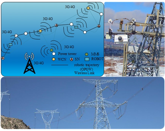
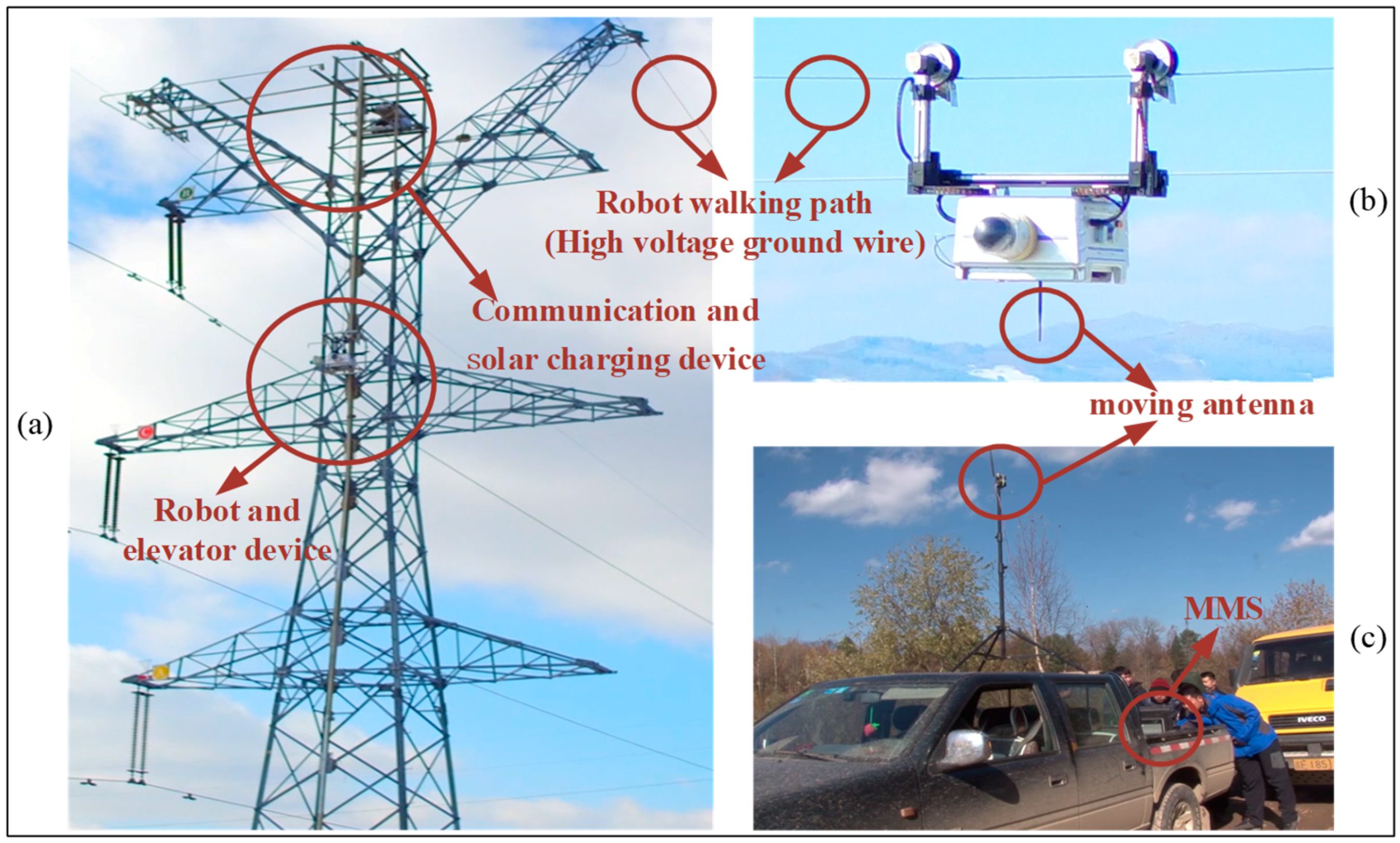
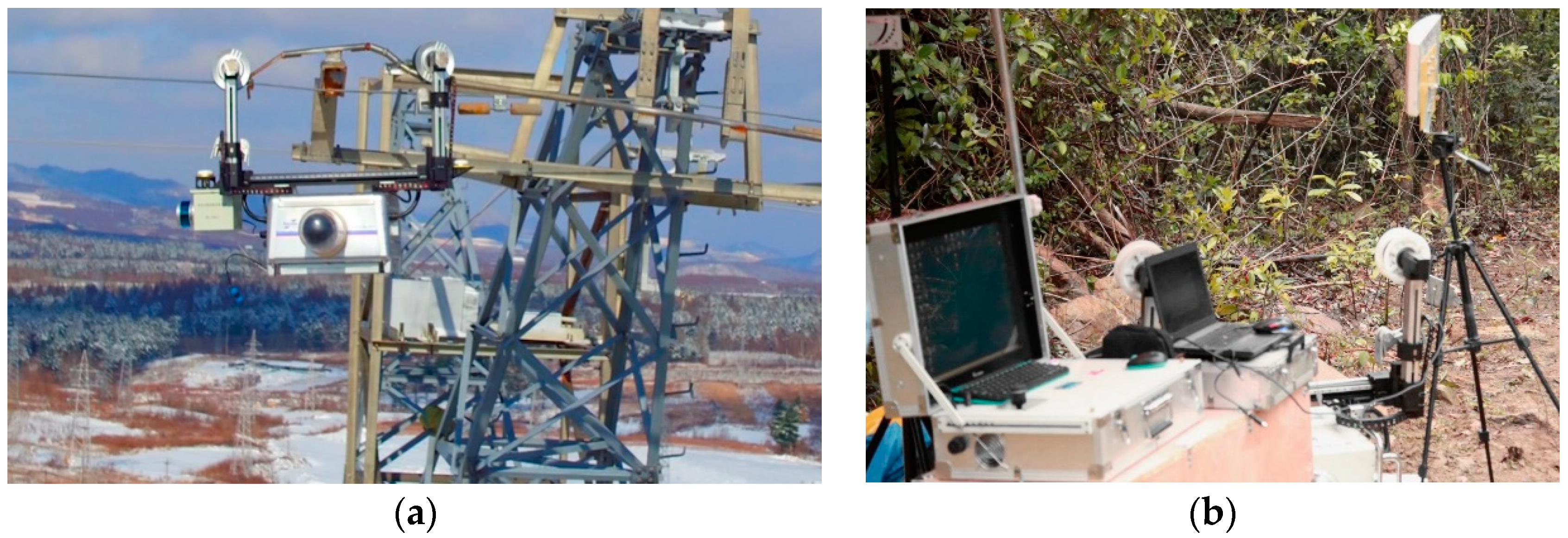
In an early piece of research, a robot inspection system was developed to realize the automatic inspection of power lines [6,7]. The inspection robot walks on the high-voltage transmission line to sense and locate faults, sending the acquired data to a mobile monitoring station (MMS) on the ground. The communication between the robot and MMS is achieved via Wi-Fi (IEEE 802. 11 n) with a moving antenna incorporated in the robot. The MMS has 3G/4G communication capabilities and it sends the data to the CMP (control and monitoring platform) through this channel. Once the CMP receives the data, it will analyze the anomalies or potential faults. The system was tested in Guangdong and Jilin provinces of China, and the project running is presented in Figure 1. However, there were some communication failures of the system in the tests conducted in the primordial forests of Jilin. Communication capabilities between the robot and the MMS were down and communication from the MMS to the CMP did not work, because of disturbance of the trees.
Real-time performance and reliability are two important indices in the monitoring systems of power grids and other scenes [8]. However, the endlessness of transmission lines makes it difficult to monitor the whole grid in real time. The real-time-based monitoring of transmission lines requires large-scale deployment of nodes to form complex Wireless Sensor Network (WSN) systems [9], which may lead to financial burden or uncontrollable risks.
Nowadays the monitoring of transmission lines is mainly based on two methods, i.e., real-time monitoring for the important components or inspection for the whole line.
The inspection of transmission lines is mainly conducted by humans, unmanned aerial vehicles (UAVs) and robots [10,11]. The main contents of inspection data are images and videos of transmission lines and surrounding environment. In remote areas, inspection of long-distance transmission lines takes several weeks or even months, and the data are usually transmitted in a delay-tolerant mode.
Robots can work in an autonomous mode and delay-tolerant communication can also meet the control requirements. Moreover, the inspection data satisfy the delay-tolerant requirements. The evaluation of transmission lines can be conducted based on the collected data such as the images or videos of loose or broken lines, and the corrosion or displacement of on-line equipment.
In order to solve the problems existing in the intelligent monitoring of a smart power grid, Robot Delay-Tolerant Sensor Network (RDTSN) is proposed in this research. The RDTSN is a trade-off solution of efficiency, cost and reliability. It combines the technical advantages of a WSN-based robot inspection system and monitoring system as well as the advantage of DTSN. It deploys a small number of robots for inspection and the static nodes for real-time monitoring. The system setup is shown in Figure 1. RDTSN aims to achieve the remote and dynamic monitoring of transmission lines.
In summary, a Robot Delay-Tolerant Sensor Network (RDTSN) is proposed to monitor the state of transmission lines for discontinuous and non-real-time network applications. The main innovations are as follows:
- Integrate advanced robot technology, WSN technology and DTSN technology to generate RDTSN. Communication nodes, along a ground wire in the air, would not be restricted by topographic situation; RDTSN can also reduce the number of fixed nodes with a small number of robots, which can balance network performance and decrease deployment costs.
- A network model for a smart grid is established, in order to better understand the interactive relationship between power grid architectures, network performances and routing algorithms. Different RDTSN scenarios are explored to determine the optimal parameters, for the balance in network performance and financial cost.
- A data delivery strategy is introduced to ensure communication security. Additionally, we try to solve the problem of availability of data traversing smart grid environments.
This paper is organized as follows. Section 2 presents some previous related work for this kind of network. The proposed method and its detailed algorithm are presented in Section 3. Section 4 shows and analyzes the simulation results of the proposed method. Section 5 provides the corresponding discussions. Conclusions are drawn in the last section.
2. Previous Related Works
In order to build an effective Wireless Sensor Network (WSN) for a smart grid, an efficient connectivity solution should be proposed, which monitors the grid status and acclimates to the remote and even unmanned areas. Delay Tolerant Sensor Network (DTSN) is a new type of sensor network architecture that can work in challenging environments, and it is a possible solution to the current scenario [12,13].
2.1. Application of Delay Tolerant Sensor Networks (DTSN)
DTSN originates from the concept of spatial communication proposed by NASA, and it was tested with Spirit and Opportunity missions to Mars [14]. In recent years, the DTSN architecture has been extended to more sophisticated communications environments such as underwater wireless sensor systems, driverless vehicle systems, remote and extreme environment monitoring, and rural communications.
For DTSN, mobile sensor nodes are often used as mobile data collectors (DMC) to process the data, or to send the data to the monitoring center. Static nodes can interact with the mobile nodes and forward messages [15]. Recently, a couple of DTSN-based projects have been actively carried out by IT companies, such as Google, Facebook and Intel [16,17]. The main purpose of these projects is to build low-cost Internet services in remote areas. Google launched its Loon project [16], using the stratospheric solar-powered balloons and ground base to build dynamic DTSN network services in remote areas. Facebook’s internet.org [17] uses local infrastructure, unmanned aerial vehicles and communication satellites to provide limited Internet services based on DTSN in remote rural areas.
Emergency response operation based on DTSN has become a promising application area in mobile ad-hoc networks (MANET) [18]. For example, in disaster scenarios, the delay/disruption tolerant network (DTN) can be used to establish emergency support communications for ease of rescue [19]. In DTSN, a message from a source node may be delivered to the destination node despite the nonexistence of an infrastructure and an end-to-end connectivity [20]. Therefore, more and more DTSN is used to solve the emergency communication problems after the destruction of telecommunication facilities.
Some research institutes have designed and developed some DMC for DTSN. Massachusetts Institute of Technology (MIT) has daknet [21], where buses or public service vehicles are used as DMC to provide Internet services in remote rural areas. In underwater wireless sensor network (UWSN), an autonomous underwater vehicle (AUV) is also used as a mobile node for message transmitting [22,23]. This research also developed a DTSN mobile node, the Inspection Robot [6,7] for constructing the grid monitoring system in remote areas.
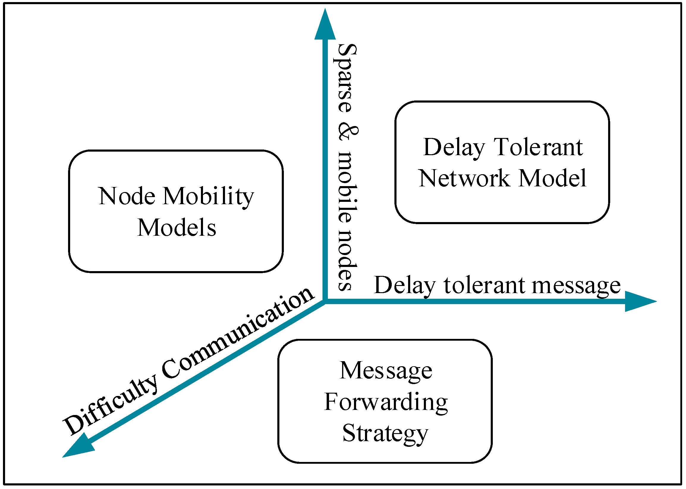
The characteristics and research directions of DTSN are shown in Figure 2. All DTSN applications have the following characteristics.
- The nodes in the network distribution are sparse and mobile.
- The application environment is complex, and ordinary communication is often not available.
- Application (monitoring data) has the characteristics of delay tolerance.
2.2. DTSN Routing Algorithms
At present, the typical data delivery strategy for DTSN is the direct transmitting algorithm [24], flooding transmitting algorithms [25,26] and social relation-based algorithms [14,27,28,29,30,31,32].
In the direct transfer algorithm, the initial network node only sends the message to the destination node and does not communicate with other nodes. Flooding strategy is one of the earliest opportunistic routing protocols. In epidemic routing [25], the network’s initiation node delivers messages to all neighboring nodes until the message arrives at the final destination. Spray and waiting routing [26] is an improved flooding data delivery strategy, where the spray and waiting routing divides the message replication and delivery into two stages. In spray stage, a copy of the message is made, and the message is distributed to the neighbor node until reaching the destination in the next phase.
The social relation routing is an intermittent connection network protocol based on the social characteristics of nodes. The typical routings are prophet routing [27] and bubbling routing [28]. Prophet routing uses the recording of encountered nodes to conduct delivery prediction, if the forwarding node’s delivery prediction is higher than its own, the message is copied and forwarded. Bubble routing is a community-based message transmitting algorithm for DTSN, where node activity is used to determine the community ranking for forwarding decisions. The other DTSN social routing protocols, such as Sim Bet [29] and People Rank [30], estimate nodes’ centrality and social distance to decide whether to forward messages through them. In the literature [14,31,32], the knowledge of graph theory and the energy model are introduced into the data delivery strategy.
3. RDTSN Model and Data Delivery Strategy
This section introduces a new type of Delay-Tolerant Sensor Network (DTSN) model and proposes a novel data delivery strategy. In order to make RDTSN work more efficiently, this research analyzes the robot’s movement along the ground wire and summarizes two types of movement models. Furthermore, the Discrete-Time DTSN mathematical model was established based on the knowledge of graph theory and the characteristics of RDTSN. Finally, the message forwarding algorithm (DTMA) is put forward for practical application.
3.1. Robot Delay-Tolerant Sensor Network (RDTSN) Model
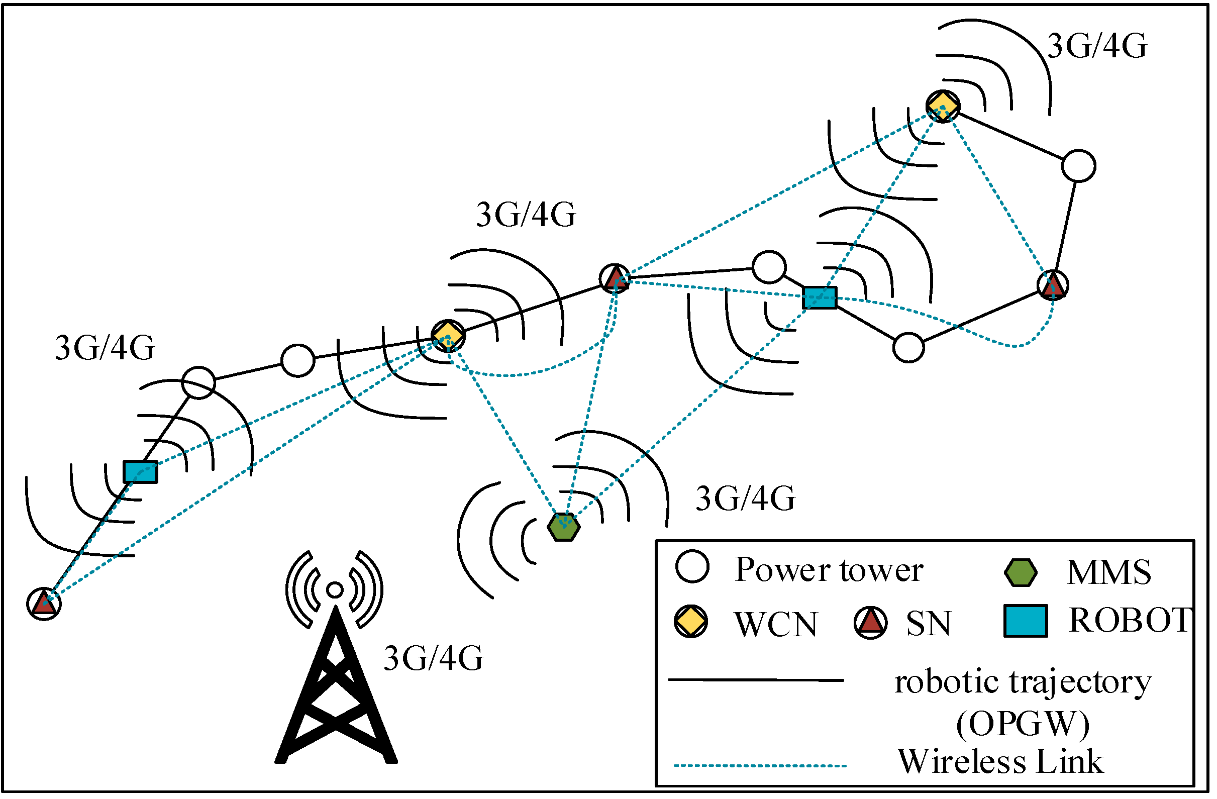
The Robot Delay-Tolerant Sensor Network (RDTSN) model is established, as shown in Figure 3. Several inspection robots, MMS and communication nodes deployed along the transmission line form an intermittently-connected mobile wireless sensor network. The communication nodes include static nodes (SNs) and wireless central nodes (WCNs). The WCN is connected to Optical Fiber Composite Overhead Ground Wire (OPGW). A data delivery strategy for RDTSN based on discrete time multi-path routing algorithm (DTMA) is proposed in this paper. RDTSN has the following properties.
- The nodes have heterogeneous communication capabilities. In order to reduce energy consumption, the communication radius of robots and SNs are smaller than R (the maximum communication radius of robots and SNs), and a WCN has two communication radii of R and C (the maximum communication radii of WCN), 2 R < C.
- The robot has heterogeneous motion speed. The robot regulates the speed according to the line environment, operative mode and energy consumption, etc.
- The inspection data has heterogeneous data capacity and transmission delay requirements.
The main idea of the strategy is to deploy a certain number of SNs and WCNs in RDTSN, so that the robot can communicate with the MMS, SNs and WCNs in a wireless way. As the robot is walking along the ground, a message can be delivered to the connectable WCN directly or forwarded via other nodes. Then, the message can be forwarded to the CMP by WCNs via optical fiber. At different times, each node can decide whether it sends a message to the neighbors or store the message in the local buffer until a better delivery path is obtained, according to its own information.
3.1.1. Motion Model of Inspection Robot
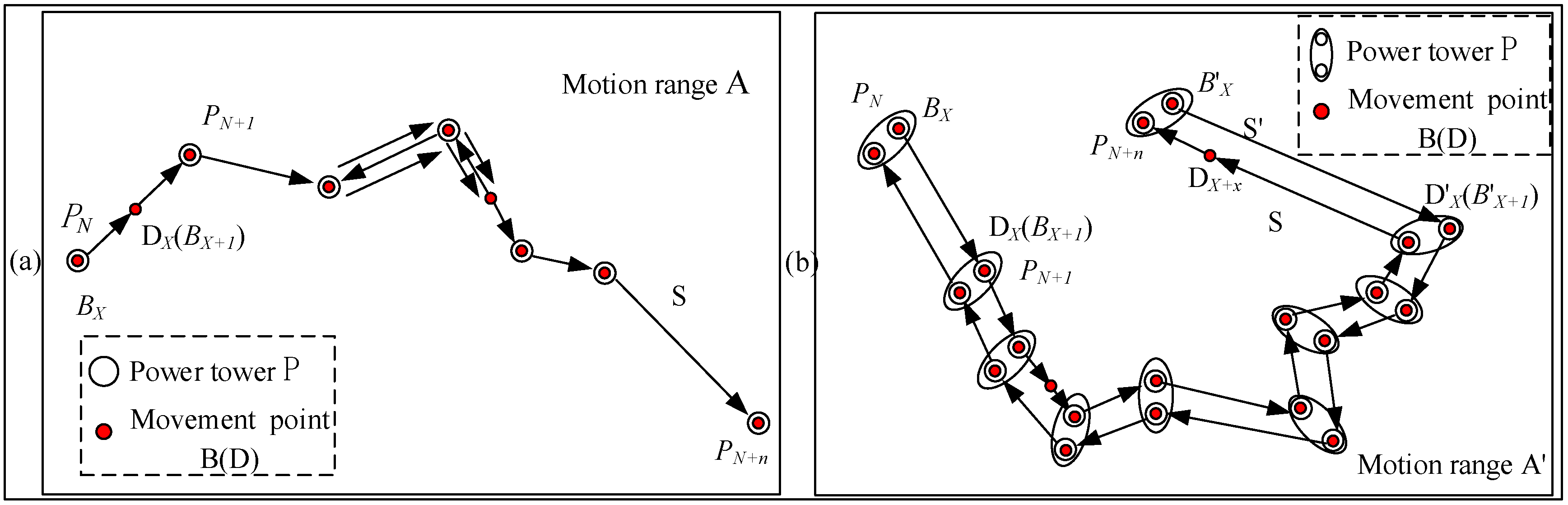
In the network model, the simplified robot movement rule is shown in Figure 4. The robot moves along the ground wire between power towers. It will maintain a rest or uniform motion between the towers of N to N + n (n, N ∈ N*). When the robot is crossing the tower, it will walk at a low speed for obstacle climbing. Its movement model is consistent with the Random Waypoint [31], but the motion is along the power line. In order to identify the more-accurate kinematic relationship of the network, this paper introduces Path-constraint Random Waypoint (PRW), Bidirectional Path-constraint Random Waypoint (BPRW) and the new movement rules.
A denotes the maximum motion range, S denotes the constraint path, P denotes the constraint point which the path S must pass through. In the network, static nodes are randomly distributed on the constraint point P. All robots follow the rules of movement and are independent of each other. Path-constraint Random Waypoint (PRW) is described as follows:
- (1)
- Randomly select the movement starting point B and end point D on the S, where the point B and D should be on the same line.
- (2)
- Set random movement rate v ∈ (vmin, vmax) as the movement rate.
- (3)
- Robot moves at constant speed on the S’s broken line of BD.
- (4)
- At point D, it takes the time of Tpause ∈ (Tmin, Tmax) to remain stationary or complete an obstacle-climbing process.
- (5)
- Repeat the movement and select the last exercise endpoint DX as the starting point for the next movement BX+1.
- (6)
- All motion paths in Path-constraint Random Waypoint do not cross.
Bidirectional Path-constraint Random Waypoint (BPRW) is similar to PRW, and it imitates the vehicle traffic and introduces two-way traffic rule. There are two parallel constraint paths in BPRW, the distribution of the constraint points P on the two constraint paths of S and S’ are consistent. On each path, the moving node can only move in one direction. It moves in opposite direction on the S to S’. Excluding the above differences, BPRW and PRW are consistent with the two motion models.
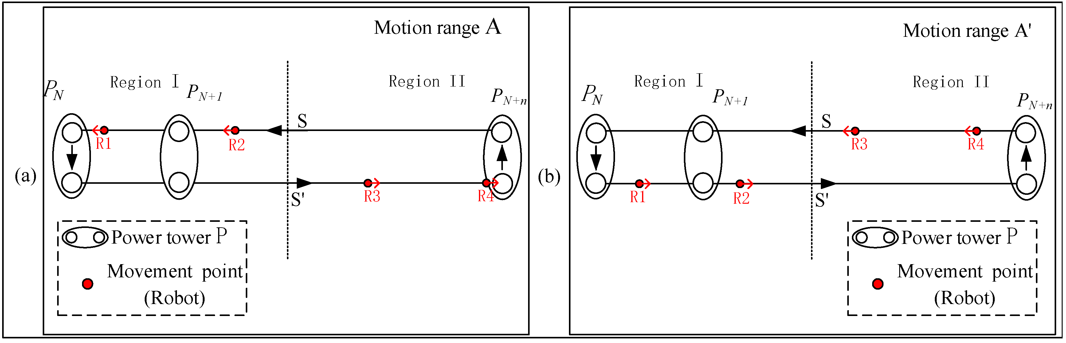
To a certain extent, the simplified rules can reflect the movement of robots in the network. However, in a multi-robot system, the motion model based on formation control will be more advantageous in reliability and efficiency. Therefore, a more capable Bidirectional Multi-robot Inspection(BMI) model is proposed. BMI model combines BPRW and formation control strategy, as shown in Figure 5 and described as follows.
- (1)
- The coordinates at unit center are the average of the multiple robots in a short time.
- (2)
- Robots perform uniform distribution in inspection tasks, as shown in Figure 5.
- The whole transmission line is divided into two heterogeneity regions.
- The robots are evenly distributed on different ground lines in the two regions.
- (3)
- The distance between any two robots on each ground line satisfies d ∈ ( − a, ), n > 1.
- (4)
- All movements follow BPRW.
In the BMI model, d denotes the distance between the two robots on each ground line; L denotes the length of each ground line; n denotes the number of robots; a denotes the accuracy of formation. All robots need to configure GPS or network-based localization algorithm. The robots can inspect all the transmission lines around it, including two ground lines. Therefore, the uniform distribution formation can achieve the best inspection efficiency.
For the inspection robot network model, high-voltage ground wire is regarded as the path-constraint S, treat power tower as the constraint point P, the robot as mobile node. Each robot acts in accordance with PRW, BPRW or BMI and they are independent of each other.
3.1.2. Discrete Time DTSN Mathematical Model
This section solves a problem of how to determine the best delivery path from one or more sources to a destination. The solution is performed based on the statistical methods of delivery probability and energy loss between nodes.
For RDTSN, as robots walk randomly along transmission lines, the network topology is unreliable and constantly changing. Furthermore, as the robots have high mobility, the entire network is locally strongly interconnected at discrete times. In order to meet the needs of the nodes (Inspection Robots, SNs or MMS) in RDTSN to transmit information to the CMP via the WCNs connected with OPGW, this paper draws on references [14,32], to introduce the graph theory to mathematically describe the above network. In the mathematical model, each link has an availability weight, which is jointly determined by link delivery probability and energy loss. The availability weights of links can change momentarily. Furthermore, the node will determine whether to send or store the message according to the weight of the link. Therefore, this paper proposes a discrete-time multi-path selection model with maximum link weights and maximum information at different time, as shown in Figure 6.
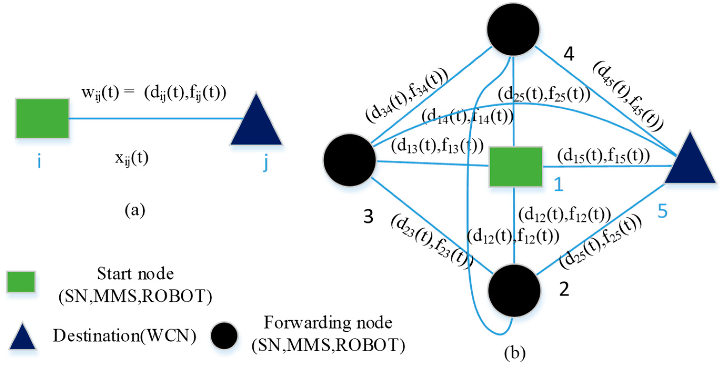
In the network mathematical model, it is assumed that the current moment is t, and the information of the network is represented by graph G (t) = (N, E). Elements of N represent the corresponding node in the RDTSN, which are a set of nodes; Elements of E reveal the physical link between those nodes, which is an edge set. At the next moment t + 1, graph G changes. The network may be represented by an extension G (t + 1) = (N’, E’) of G (t), as shown in Figure 7. The graph G contains all the information of the network. In addition, Equation (1) is used to calculate the weight function wij(t) of each edge. It shows the change rule of the links’ availability weight over time. In each new extension G (t + n) of the network, a node makes decisions to forward or store the messages based on the elements and relationships of the current graph. Pij(t) is the best path for the message to be transmitted from the source node to the target node. One path can be jointly created by the physical links of different nodes at several discrete moments.
At each moment, an aik(t) is given, which represents the link availability probability between node i and node k. Equation (2) is used to obtain the variable dij(t) denoting the delivery probability of the source node i forwarding to node j, through node k. The variable dki(t), in Equation (2), denotes the delivery probability from node k to node j. At time t, Ei(t) denotes the total energy of node i, eij(t) denotes the energy consumption of message delivery by path Pij(t), and the variable fij(t) denotes the node survivability, which is given in Equation (3). In Equation (4), the objective function of the network mathematical model is constructed. As the description of the objective function, messages are forwarded by nodes at different discrete moments. It ensures that the appropriate message delivery probability, energy consumption, and message delay are obtained. The constraints on network traffic and energy consumption are given in Equations (5)–(8). Each node has a certain storage capacity. bi denotes the buffer size of node i, bij denotes the information capacity of link Pij(t). In the model, xij(t) is the target variable, which represents the data flow between node i and node j. The discrete time variable δt(t) represents the time interval of each discrete time period, i.e., the maximum duration of the current link.
Objective function:
Constraints:
3.2. Discrete-Time Multi-Path Routing Algorithm
This section describes a discrete time multi-path routing algorithm (DTMA), which is similar to the prophet algorithm. The prophet algorithm predicts the probability of message delivery, depending on the historical data of the encountered nodes. The shorter the encounter time interval of the nodes, the more the encounter times, and the higher the probability of predicting delivery. However, the inspection movement of the robot is different from the common random motion. After the robot meets a node, the probability of the return movement is low. The return movement is carried out only when the robot is inspecting. In particular, in the BPRW and BMI movement model, the robot cannot have a reverse motion. Furthermore, the layout of SNs and WCNs is sparse along the long-distance transmission line. The historical data that the robot meets with other nodes change too slowly. Therefore, it is impossible to accurately describe the relationship between the network change and the message delivery probability by calculating the historical data of the encountered nodes. The method of the prophet algorithm is no longer applicable in this situation.
DTMA is similar to the prophet algorithm, and it is based on the nodes’ social and historical information. Furthermore, it is combined with the discrete time DTSN mathematical model. In DTMA, the prediction of message delivery rate depends on the exact calculation of link availability. The availability of links between nodes is determined by the signal strength of nodes in the wireless networks [8]. When the signal strength reaches a certain threshold Sr, the wireless link is connected. In addition, the link availability probability between node i and j equals 1, as shown in Equation (9). Each node records the intensity of the signal between itself and the neighbors at different time. If the current signal strength Sij(t) is lower than the threshold value Sr, the value aij(t) can be calculated by discrete-time weighted average of the signal strength Sij(t), as shown in Equation (10). This value not only reflects the nodal motion in the front stage, but also highlights the influence of the node’s current position. For example, as the node is away from the others, the value of aij(t) can be much smaller. If node i hovers around node j for a period, the value of aij(t) will become larger. This means that the message will more probably be transmitted to node j. If node i is always away from node j, the value of aij(t) will be very small. In addition, the discrete time variable δt(t) has a strong negative relationship with the value of aij(t).
In addition, this paper combines the DTMA with the discrete time DTSN mathematical model. Each node can obtain a better transmission path based on its own information, as shown in Figure 3. The message is transmitted from one node to the appropriate neighbor node, when the condition is allowed. Or messages will be stored in the local buffer, until the transmission conditions are satisfied. The process of message delivery is as follows.
- Firstly, the node calculates the availability probability according to the social and historical information.
- Secondly, the message delivery ratio and the node survivability are calculated according to the graph information in the mathematical model.
- Thirdly, for determining the weight function wij(t) of each edge, the message delivery ratio and the node survivability need to be adjusted.
- Finally, the node determines the message forwarding process based on the objective function and the constraint conditions.
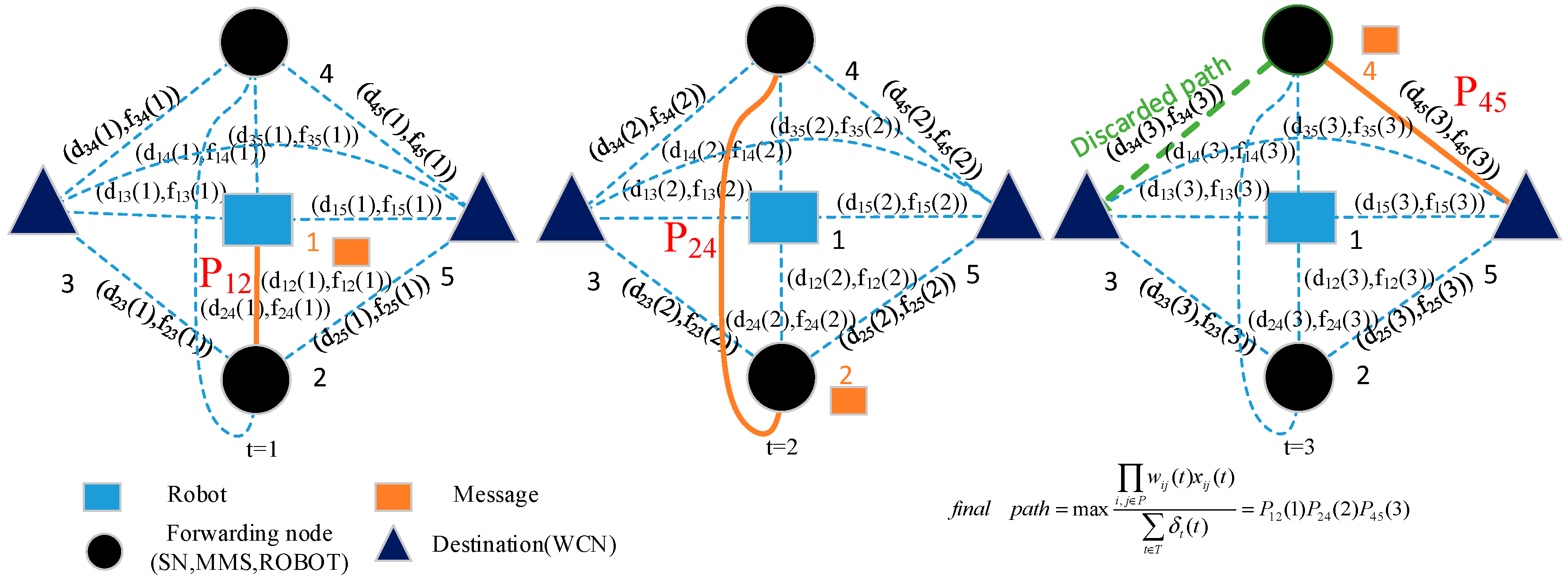
In RDTSN, a special scene is identified, as described in Figure 8. A number of WSNs are deployed in the network, leading to the formation of many homogeneity wireless destinations. In the process of message delivery, the transmission paths of different endpoints need to be compared, and the best destination is determined. Unlike common routing algorithms, DTMA is allowed to change the message destination. The determination of the message’s ultimate destination usually occurs at t = 3 in Figure 8. At this point, the message transmission paths of different endpoints are compared based on the method described above. The message is sent to the best path to satisfy the objective function and constraint conditions. Finally, the node independently completes the optimization of the message destination.
Figure 8 gives an example of the DTMA at work. The robot forwards the message to the destination (WCN) via 3 steps, which are listed as follows.
- Step 1:
- The robot (node 1) transmits the message to the relay node 2 based on the obtained best transmission path (P12).
- Step 2:
- The relay node 4 forwards the message to another relay point by P24.
- Step 3:
- The relay node calculations the best path (P45) based on objective function and sends the message to the best destination (WCN, node 5). In addition, this also means eliminating the possibility of node 3 as the destination.
Finally, the message is sent via WCN (node 5) to the CMP connected to the OPGW.
The DTMA solves the problem of determining the best delivery path by matching the objective function. Particularly, the choice of delivery paths comes from one or more sources to a variable destination. The Discrete Time Multi-Path Routing Algorithm (DTMA) is shown as pseudo code in Algorithm 1.
| Algorithm 1. DTMA for every node in the network. |
| 1: node start (initialization) |
| 2: broadcast ID |
| 3: listen for neighbors’ IDs |
| 4: wait for messages () |
| 5: if message receives in queue then |
| 6: update mean time between contacts |
| 7: update availability probability |
| 8: update survivability and delivery probabilities |
| 9: update availability weight |
| 10: if neighbor requests delivery probability then |
| 11: if message destination = my ID then |
| 12: save message in memory and delete it from queue |
| 13: else if message destination = others’ ID then |
| 14: check neighbors’ availability weight to destination |
| 15: send a copy of the message to the best availability weight neighbor |
| 16: if is no availability weight then |
| 17: store message in buffer until a path to destination appears |
4. Results
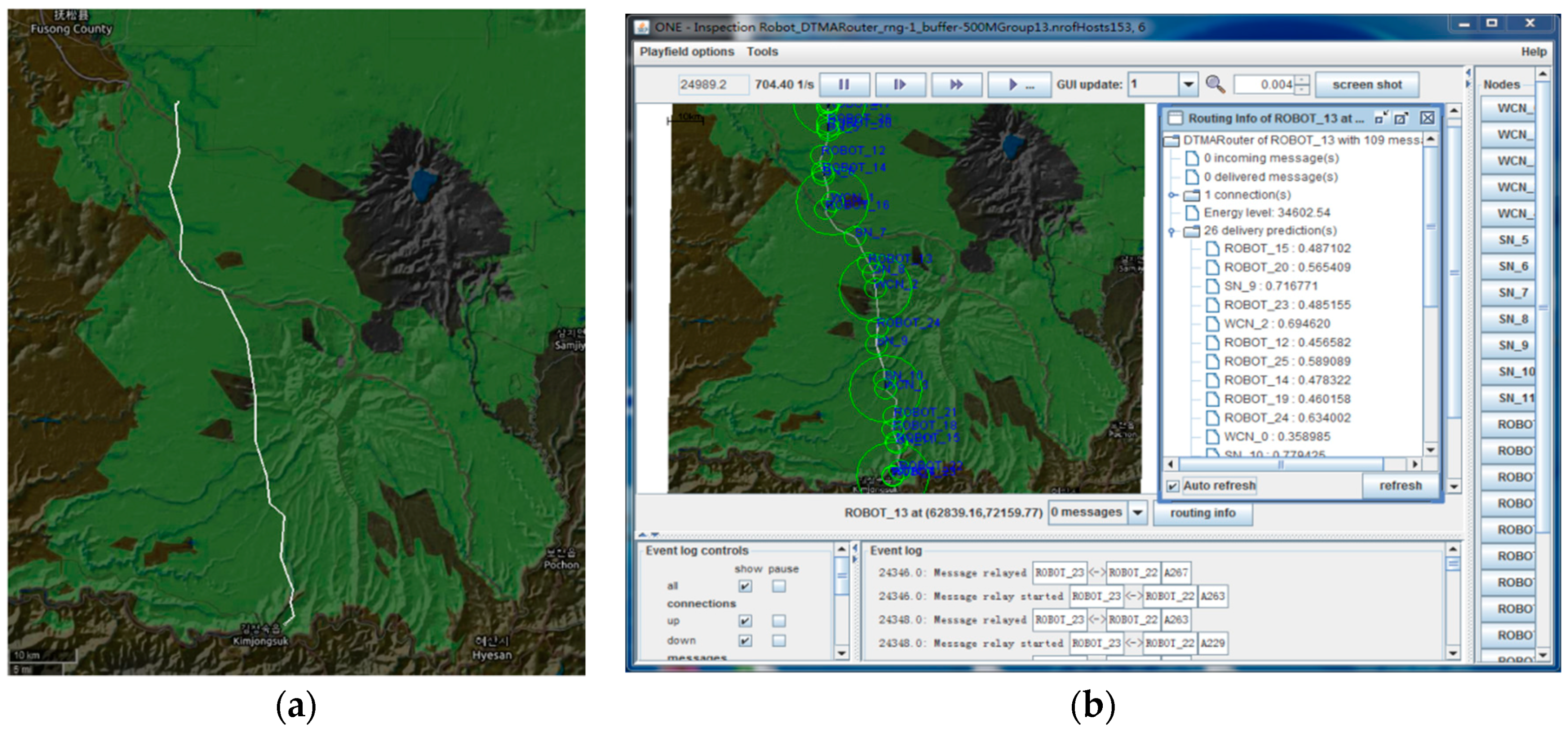
This section used the Opportunistic Network Environment (ONE) simulator [33] (The ONE version 1.6.0 was developed at Aalto University, Finland, 2015) to obtain the results of the DTMA in the RDTSN. The simulation test was performed on the inspection robot project in Jilin, China. That is a 220-kV high-voltage transmission line with a length of about 120 km. It traversed virgin forest and unmanned area and ended in the border area of China and North Korea. This paper used Open Street Map [34] to get local geographic and traffic information. In addition, the moving path (transmission line) of the inspection robot was depicted in the map. Then the simulation experiments were carried out based on the test environment in the ONE simulator. The map information and simulation interface of the RDTSN are shown in Figure 9. In the Figure 9, the high brightness white lines indicate transmission lines, the dark lines indicate local traffic information, the green and brown areas indicate vegetation coverage, and the blue area indicates water area. The highlight green circle represents the network node, and the radii of the circle represents the communication range in the simulation interface (Figure 9b).
The DTMA with multiple RDTSN scenarios was tested. Then, DTMA was compared with three most popular DTSN routing algorithms, namely, Prophet V2 [27], Epidemic algorithm [25] and Spray and Wait algorithm [26]. In order to build RDTSN scenarios, 5 WCNs and 7 SNs are configured along the transmission line, as shown in Figure 9b.
4.1. Results for the Default Parameters
For the scenarios, the coverage area of the network is 74,500 × 143,400. All nodes have wireless communication capabilities similar to IEEE 802.11n, and the transmission rate is 8 Mbps. The default transmission range of the WCNs is 10 km. The SNs and the robots’ default transmission range are 3 km. The default buffer size of nodes is 500 M. In practice, the number of robots is limited by cost, and the simplified motion model can not only improve the efficiency, but also do not affect the results. The default number of robots is 5. The default motion model is BPRW, with a movement rate of 3–5 m/s. The initial power of both the WCN and the SN are 100 Ah, and the robots are 57 Ah. The message generation of each node follows the Poisson process. The message arrival time is 60–120 s in the robot, and 1800–3600 s in the SN, with a message size of 2 m. The messages are directly delivered to WCNs or forwarded by other nodes. The above parameters are based on actual robots and transmission lines. Each simulation’s run time is 86,400 s, where the 24-h running results of actual network was simulated. 200 simulations were performed for each scenario. The default simulation parameters are shown in Table 1. All routing parameters have been optimized, see Section 4.2 for more details.
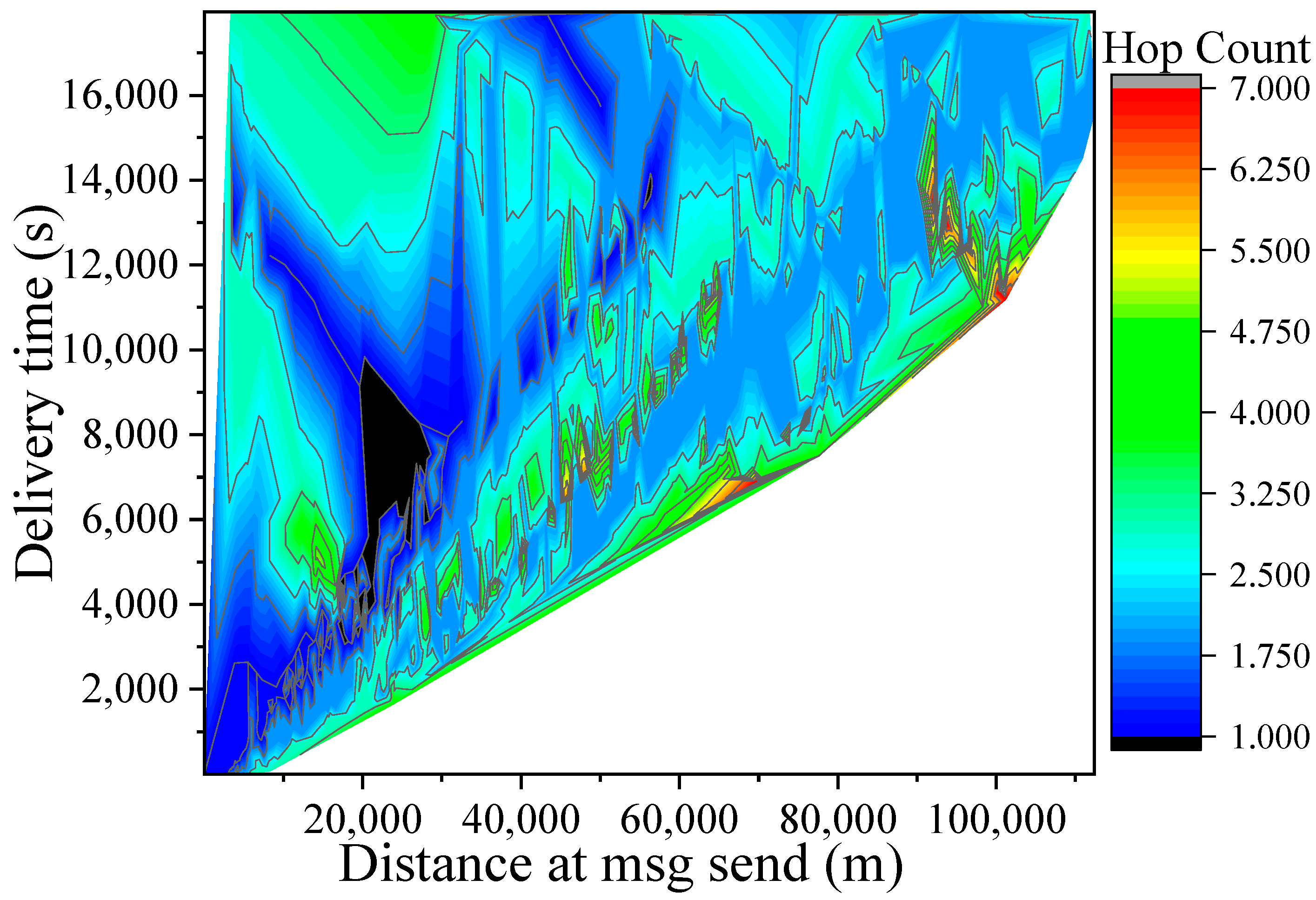
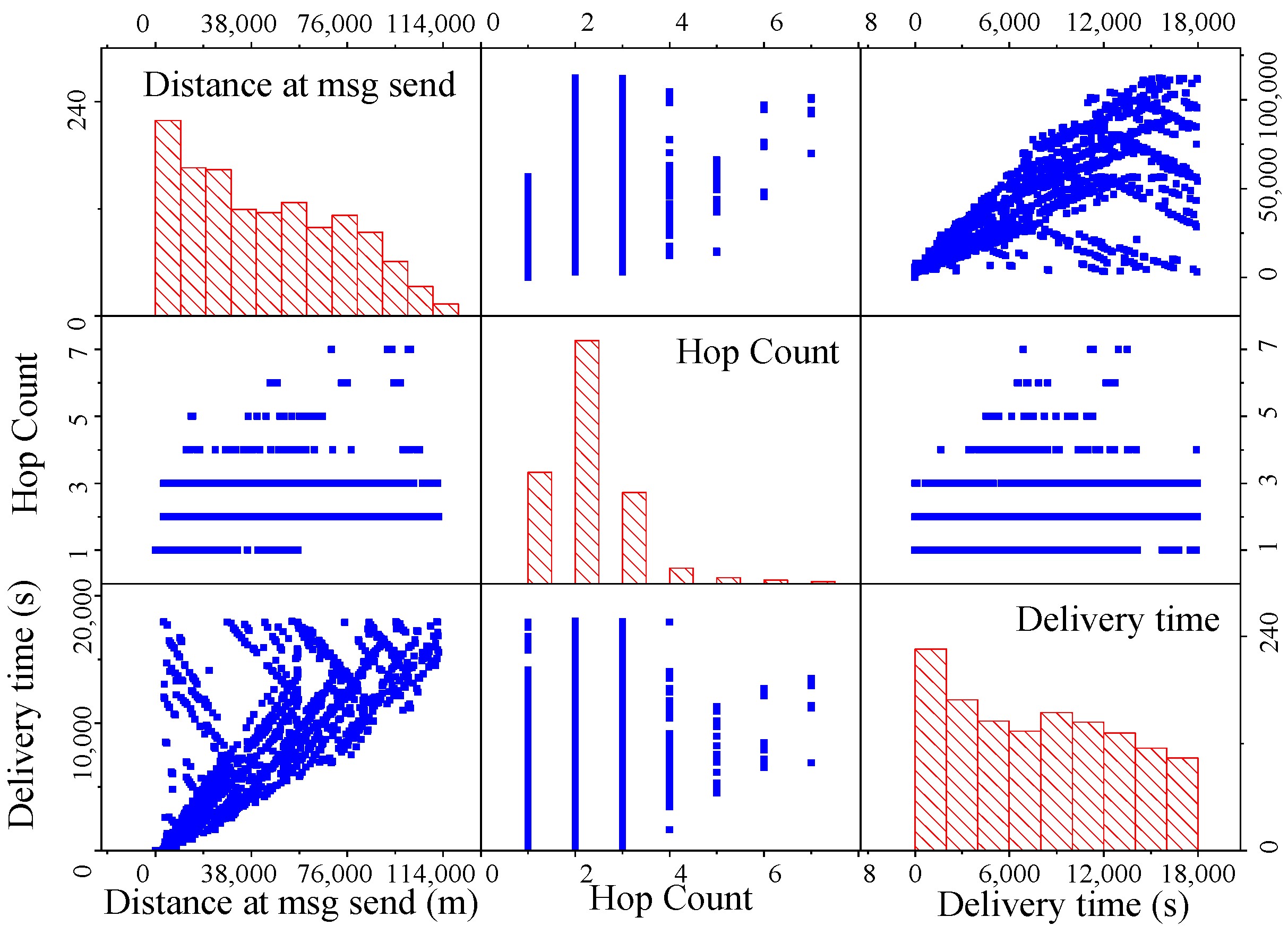
The statistics on the network message delay, delivery distance and hop count were gathered under the default conditions. The results and statistical analysis data are shown in Figure 10 and Figure 11. The amount of message delivered sharply dropped with the increase in node distance, as the distance exceeded 80 km. The average hop count in the network was about 2.7, and most of the hop count in the distribution was 2. The network’s average message delay was about 7600 s, and the nodes with lower delay were denser.
4.2. Results for the Change of Routing Parameters
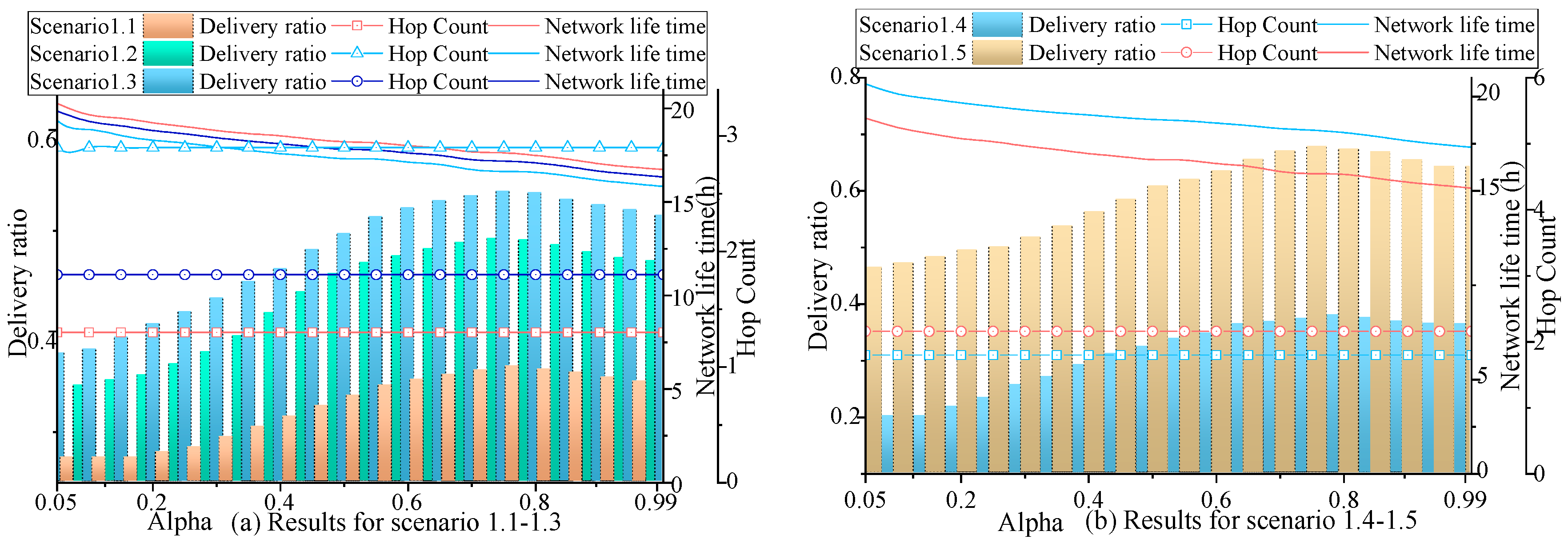
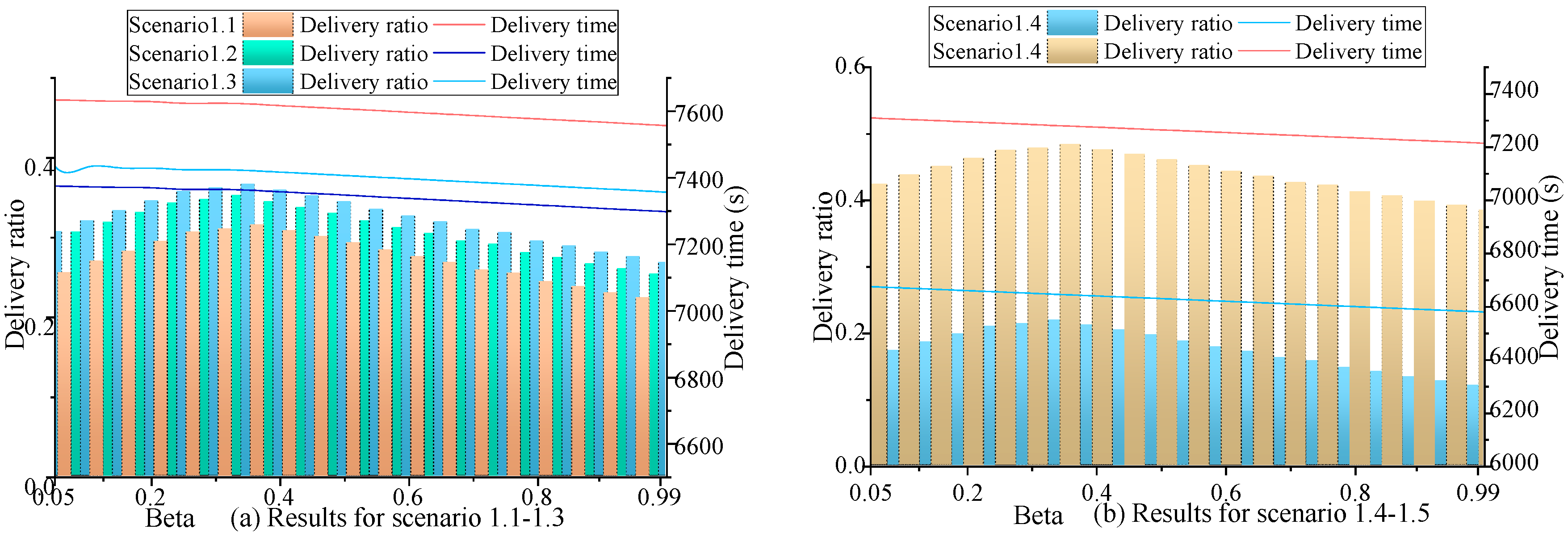
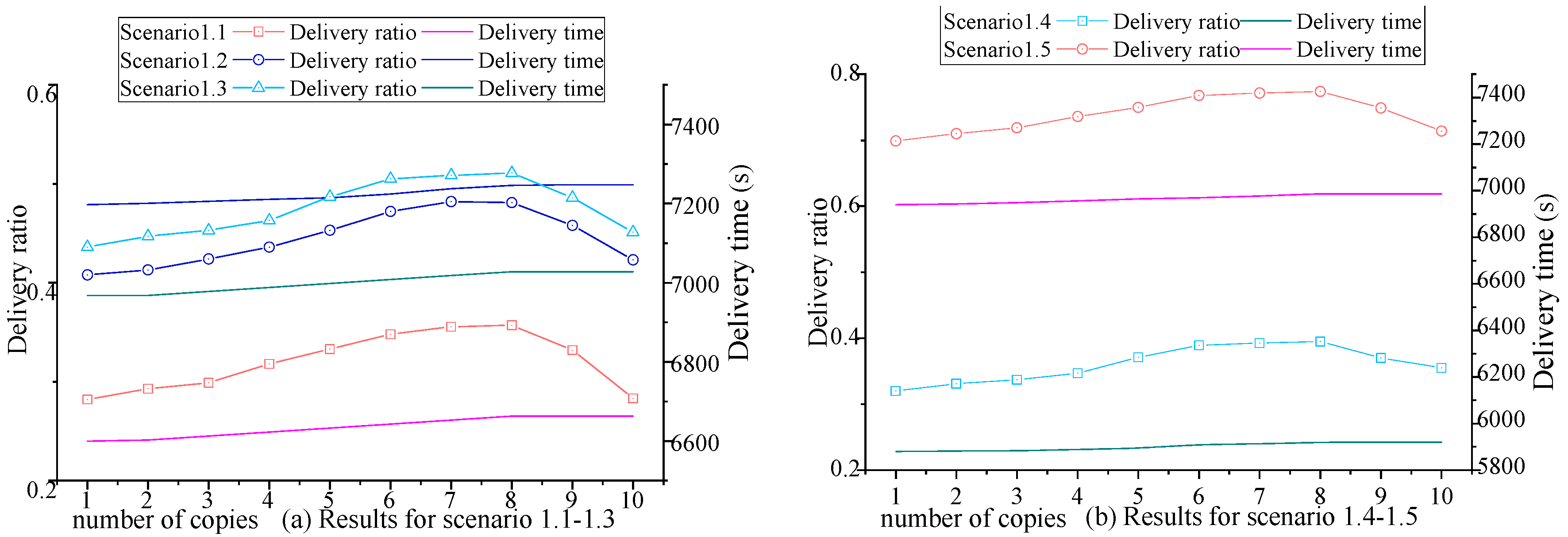
The values of the routing parameters are changed and the number and speed of the robots are adjusted in Scenario 1. The alpha of DTMA and beta of Prophet V2 varies from 0.05 to 0.99, with an increment of 0.05 for each simulation run. The number of copies of Spray and Wait varies from 1 to 10, with an increment of 1 for each simulation run. The configuration of the number and speed of the robots in Scenario 1 are as shown in Table 2. In different scenarios, the robots’ performance changes with the configured parameters, as presented in Figure 11, Figure 12 and Figure 13.
As can be seen in Figure 12, for alpha values of DTMA between 0.05 and 0.65, there are no significant differences in all variables except message delivery ratio. For alpha values from 0.7 to 0.9, the hop count remains steady but the network life time and the delivery probability decreases sharply. These results show that choosing an adequate alpha value is a critical step, and that the alpha value between 0.65 and 0.8 most likely provides the best trade-off between network life time and delivery probability.
In Figure 13, for the beta values of Prophet V2 ranging from 0.2 to 0.4, significant differences exist in the message delivery ratio. For the beta values from 0.2 to 0.37, the delivery probability goes steadily up, and when beta values are greater than 0.37, delivery probability begins to fall. In the simulation, the network delay keeps declining with the increase of beta values.
The results of the change in the routing parameters of Spray and Wait are shown in Figure 14. In multiple scenarios, with the change of number of copies, network performances show a common feature. As the number of copies increase, the delivery ratio and message delay rise steadily, until when the number of copies is greater than 8, delivery probability begins to drop sharply.
To sum up, this paper selects the optimized routing parameters based on the change rules of network performance. The parameter alpha of DTMA energy consumption is set to 0.78, and the optimized transfer factor of Prophet V2 beta is 0.36. For Spray and Wait, binary-mode mode is used and the initial number of copies is set to 8.
4.3. Results for the Change of Network Parameters
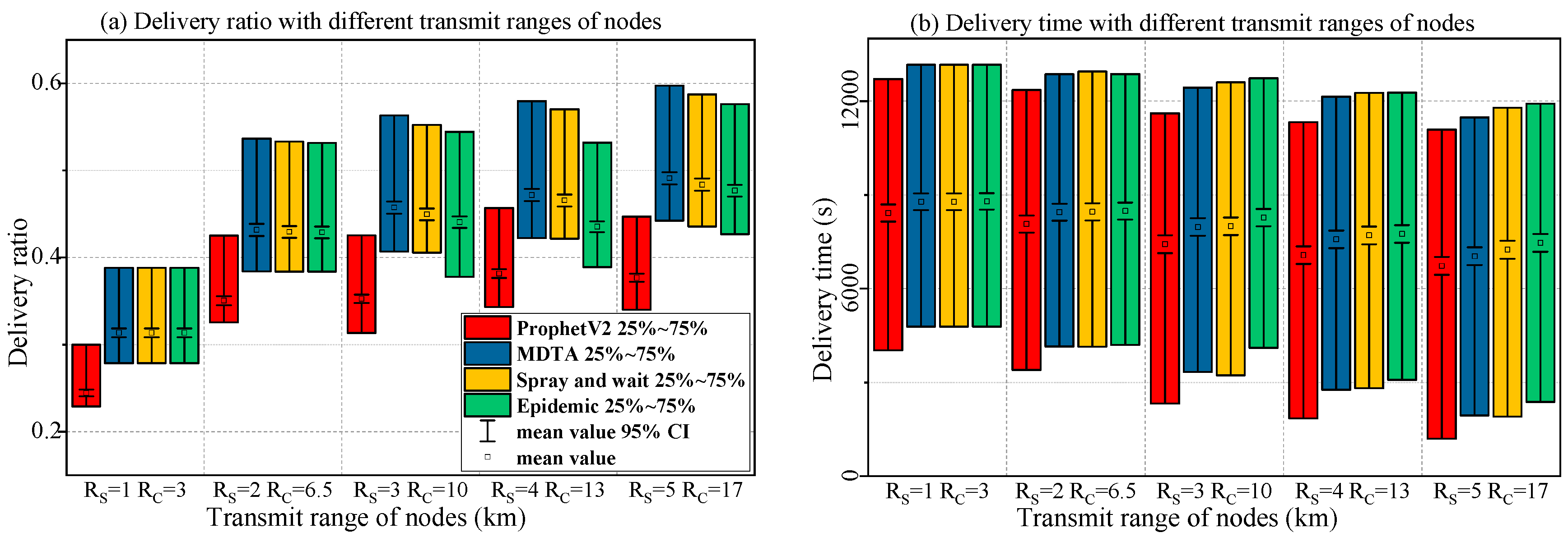
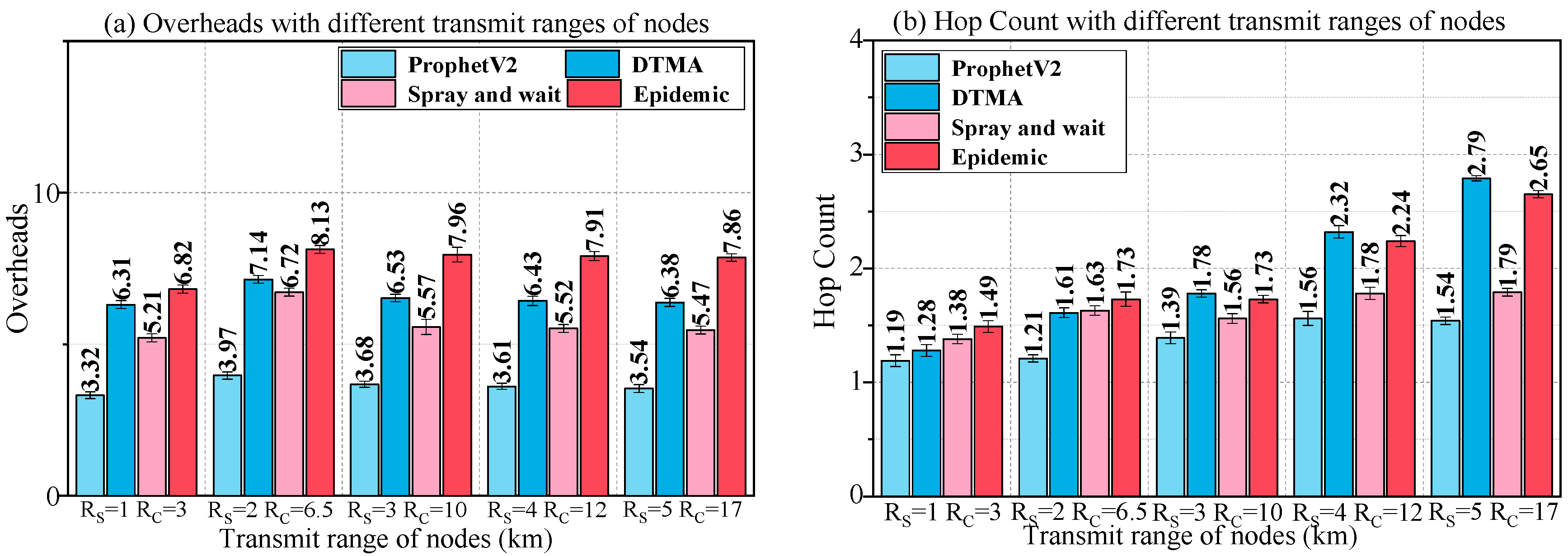
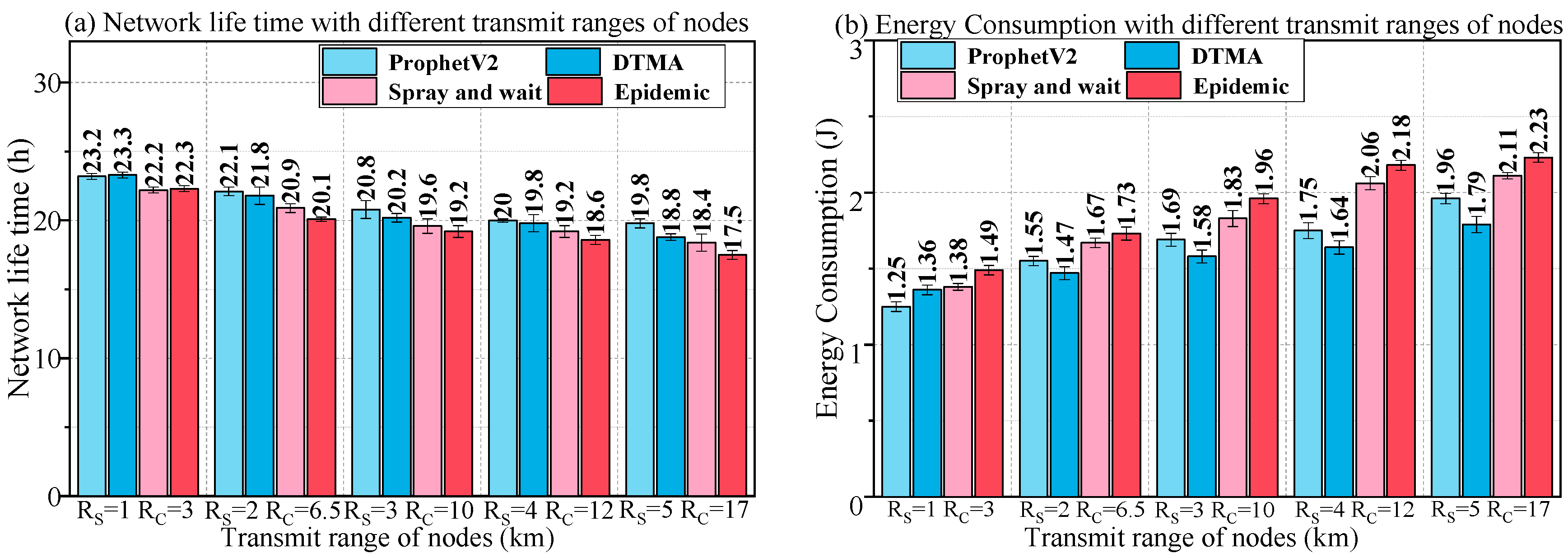
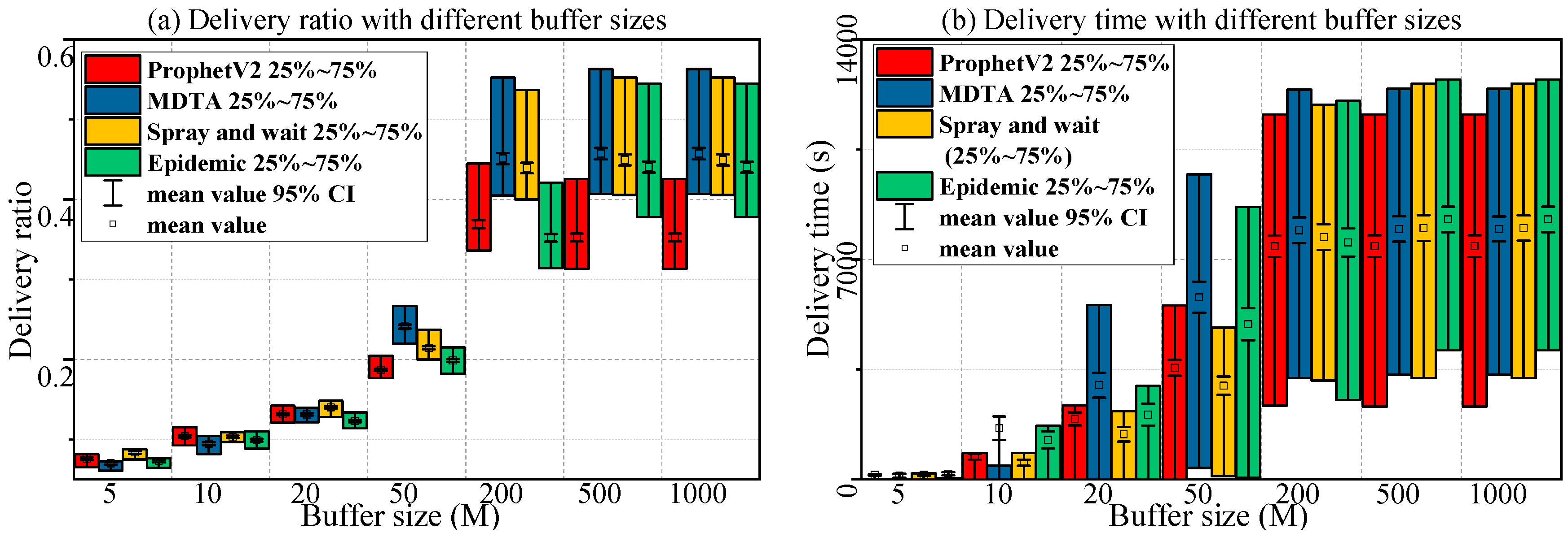
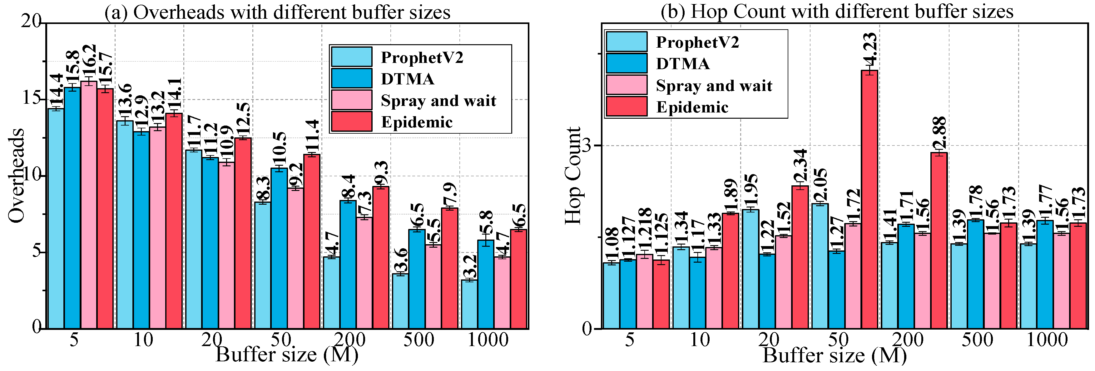
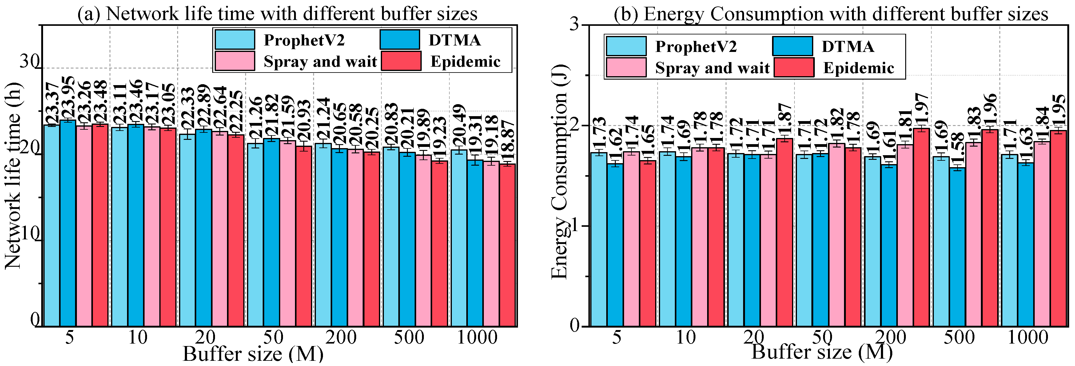
In Scenario 2, comparison was performed on the dynamic characteristics of four routing algorithms in different network environments. In different scenarios, we have recorded message delivery ratio, message delivery time, overheads, hop count, network life time and energy consumption. The 95% confidence intervals are calculated for every result and they are plotted on the figures. In sub-Scenarios 2.1–2.2, several parameters are changed, such as the transmission range of nodes and the buffer size. Each scenario has changed one or two parameters from the default values. 200 simulations were performed for each scenario. The parameters in Scenario 2 are configured as shown in Table 3 and Table 4. Results of Scenario 2 are shown in Figure 15, Figure 16, Figure 17, Figure 18, Figure 19 and Figure 20.
Results of Scenario 2 show that the proposed method performs as well as the other routing protocols in most cases or even better in some respects such as the delivery ratio and the energy consumption. We can see from Figure 15a and Figure 18a that the delivery ratio acts as an increasing function of all parameters for all protocols in Scenario 2. The message delivered in the proposed DTMA increases as the parameters increase, followed by Spray and Wait and Epidemic. Similarly, the energy consumption acts as an increasing function of all parameters for all protocols in Scenario 2. DTMA shows the minor energy consumption as the parameters increase, followed by Prophet V2 and Spray and Wait (Figure 17b and Figure 20b).
We can also see from the results of Scenario 2 that the delay shows different trends with the increase in all parameters of four protocols. Firstly, the delay is positively related to the buffer size (Figure 18b); secondly, it is negatively related to the transmission range of nodes (Figure 15b). In most cases, Prophet V2 shows the minor delay, followed by DTMA and Spray and Wait and Epidemic.
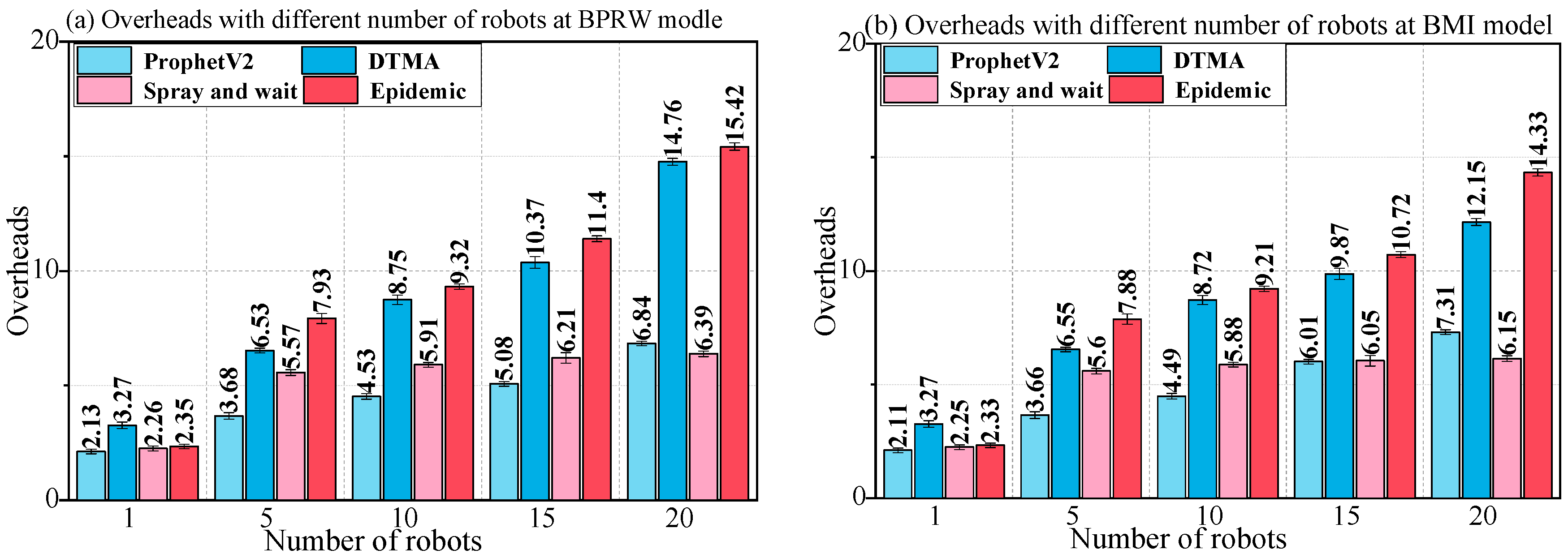
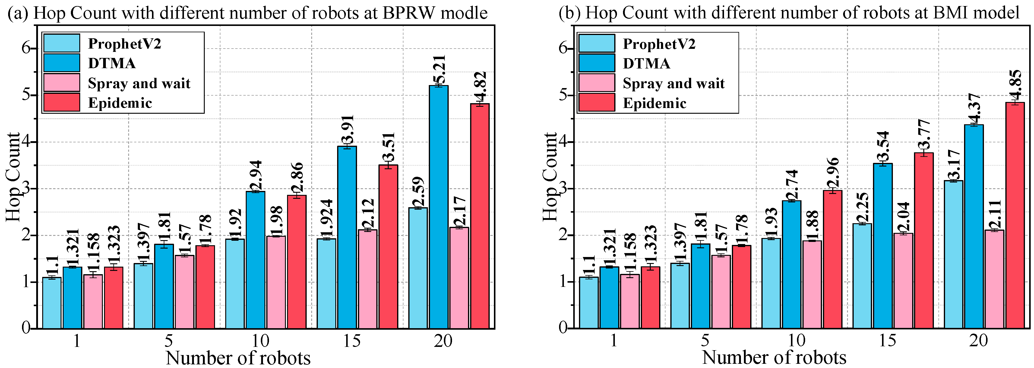
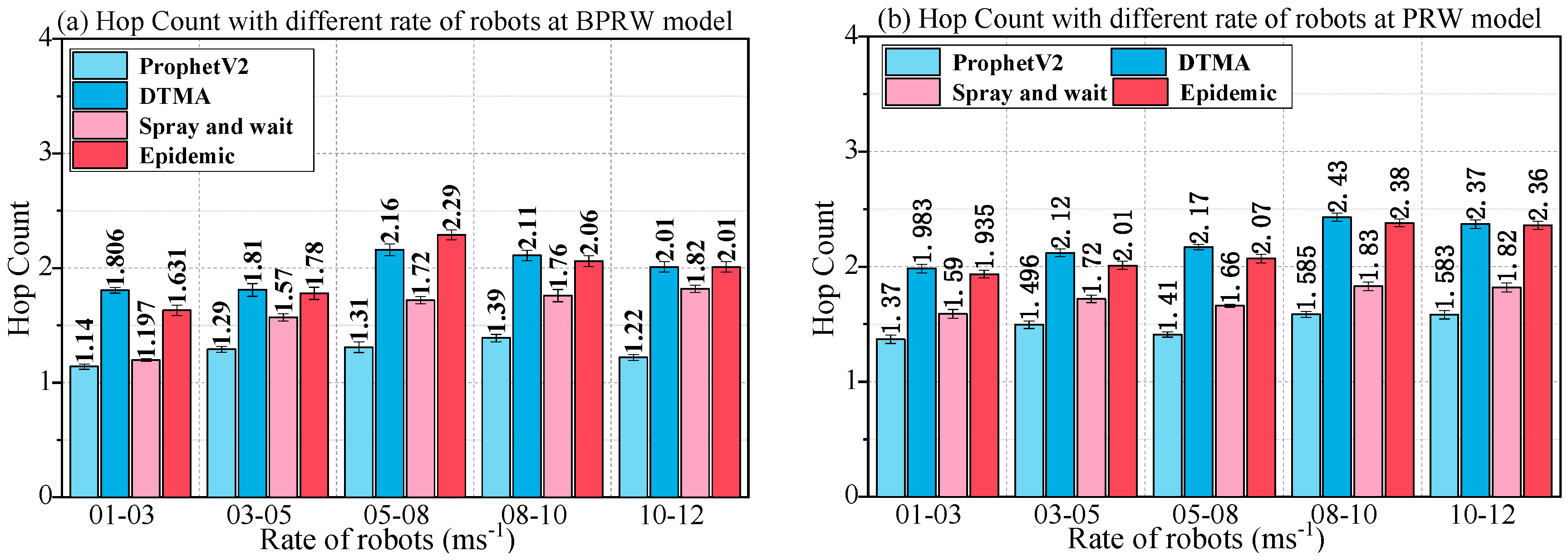
For Scenario 2, hop count performance is presented in Figure 16b and Figure 19b. DTMA and Epidemic try to deliver more messages through more hops, while Prophet V2 and Spray and Wait cannot change the number of hops when the parameters change.
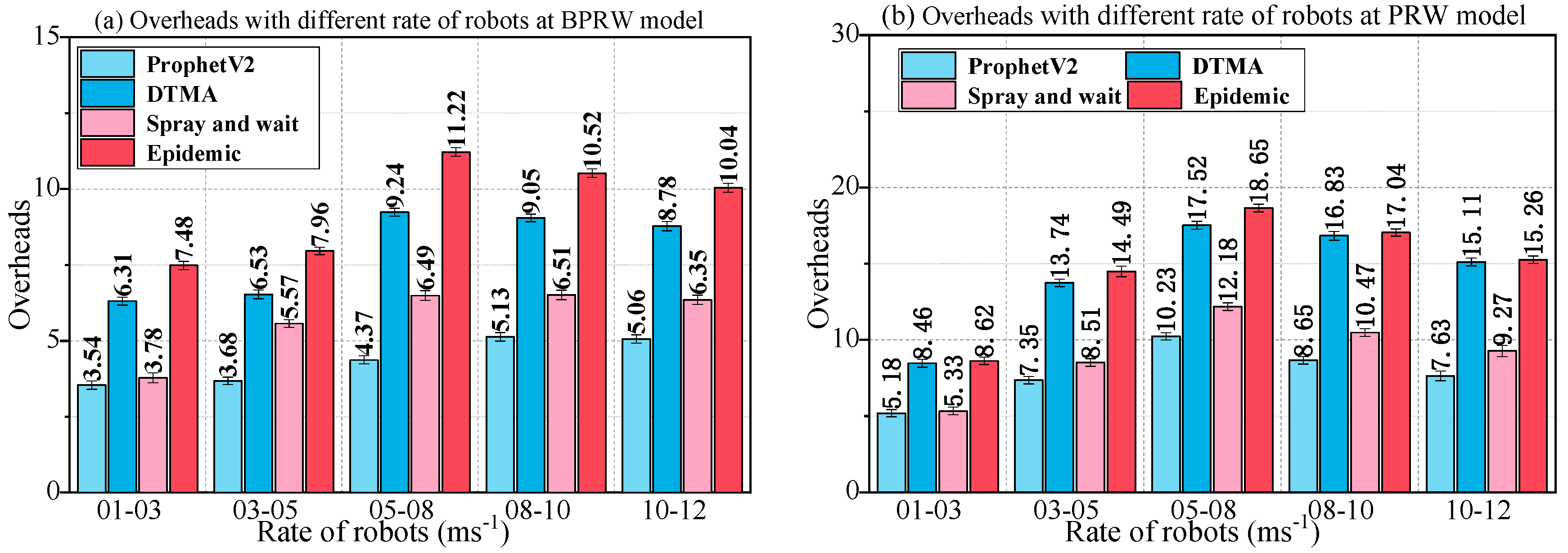
Regarding overheads, Scenario 2 shows that the proposed DTMA and Epidemic has the worst performance by replicating more messages than it is delivering. Prophet V2 has the best performance as the number of robots increases, followed by Spray and Wait. For all sub-scenarios, all protocols have a similar overhead performance except Prophet V2’s smaller overhead in general.
4.4. Results for the Change of Movement Model
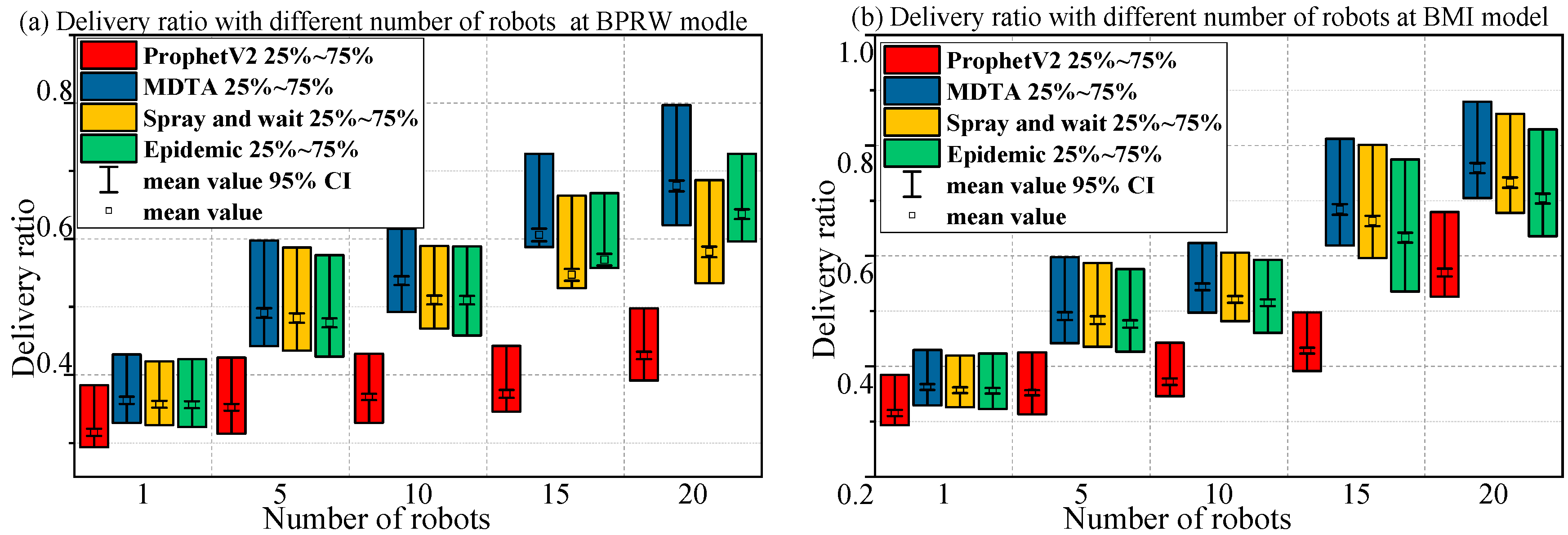
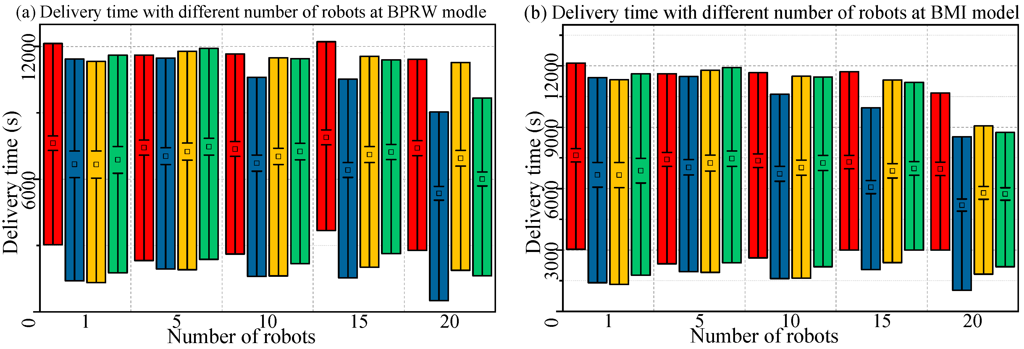
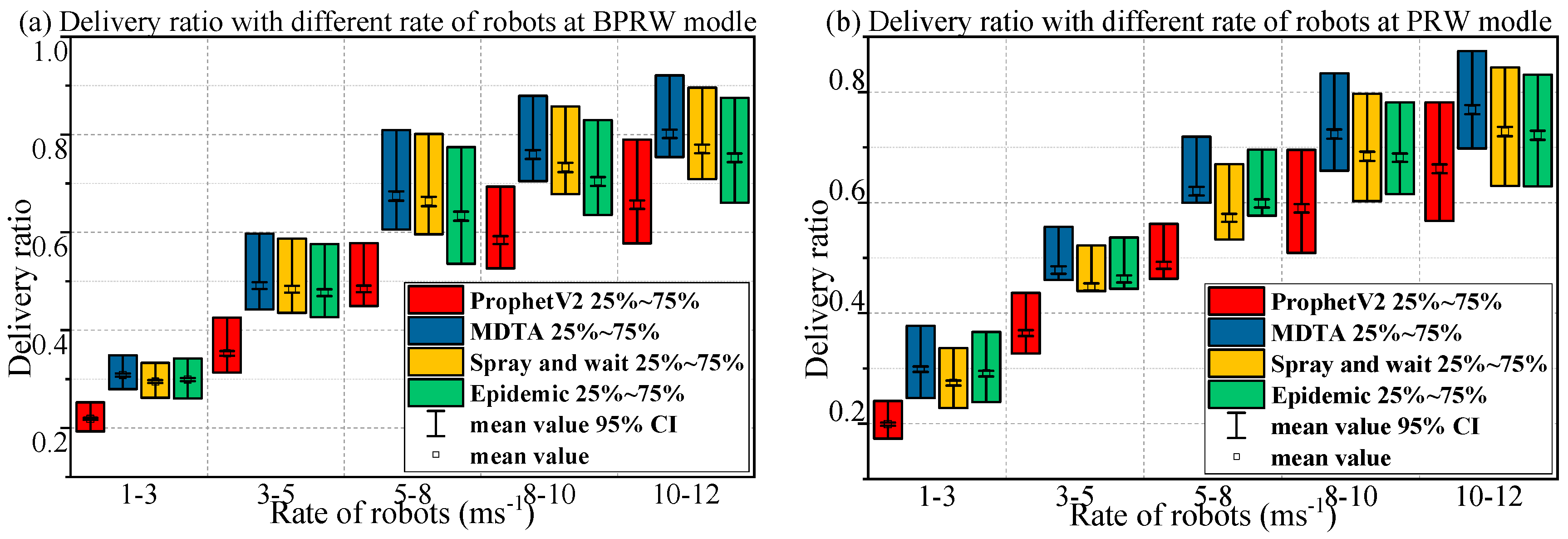
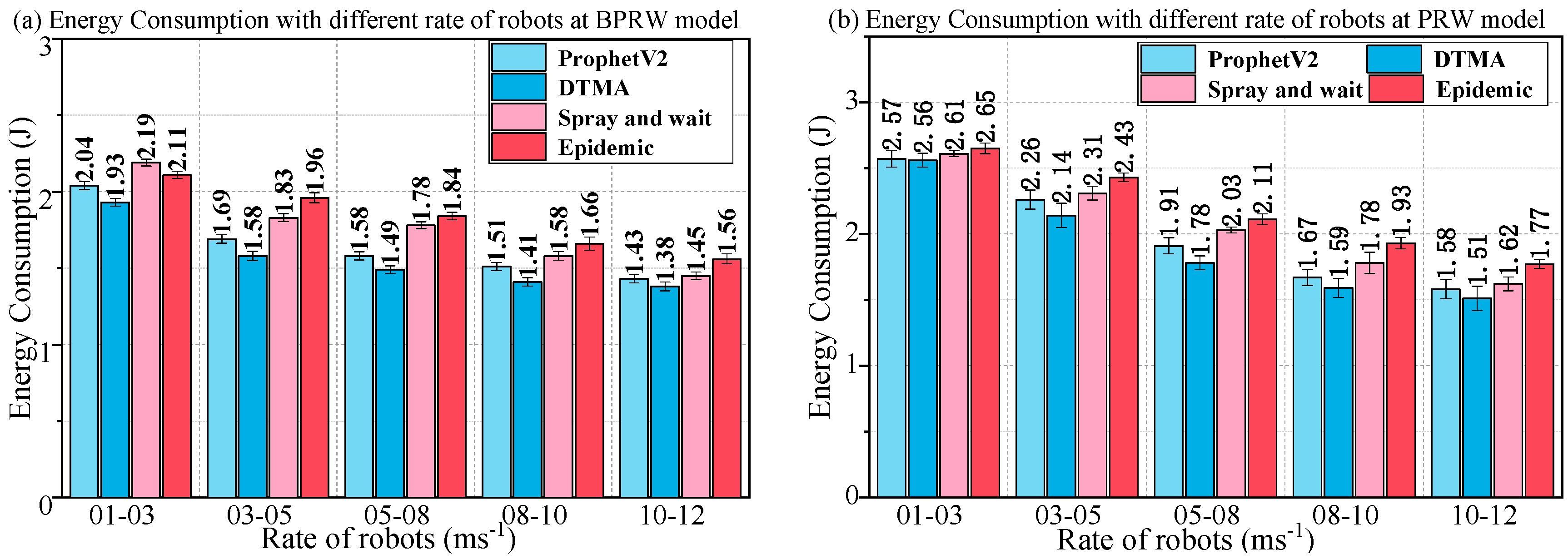
In order to investigate the influence of different movement models on several routing algorithms, Scenario 3 is constructed. Robots moved under different movement models of BPRW, BMI and PRW, and the number or rate of robot was increased from 1 to 20, or from 1–3 m/s to 10–12 m/s. In different scenarios, we have recorded message delivery ratio, message delivery time, overheads, hop count, network life time, and energy consumption. The 95% confidence intervals were calculated for every result and they were plotted on the figures. In sub-scenarios 3.1–3.4, several parameters were adjusted, such as number or movement rate of the robots and the movement model. The parameters in Scenario 3 are configured, as shown in Table 5, Table 6, Table 7 and Table 8. Each scenario has changed one or two parameters based on the default values. 200 simulations were performed for each scenario. The results for Scenario 3 are shown in Figure 21, Figure 22, Figure 23, Figure 24, Figure 25 and Figure 26.
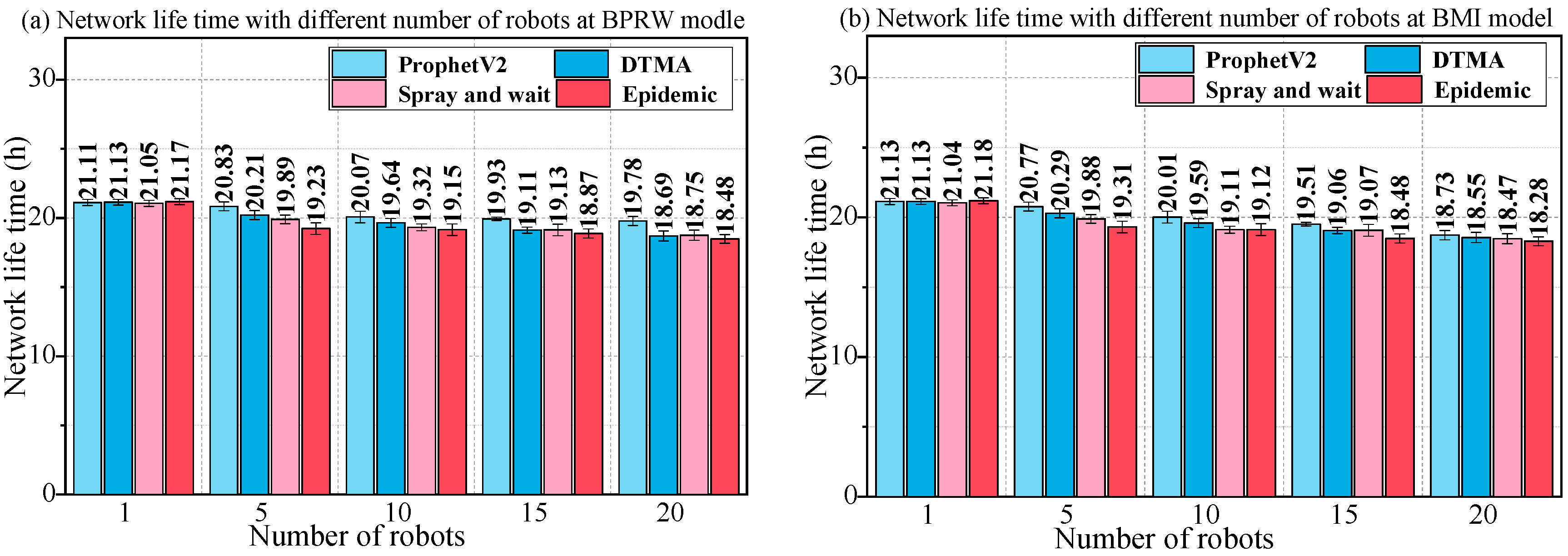
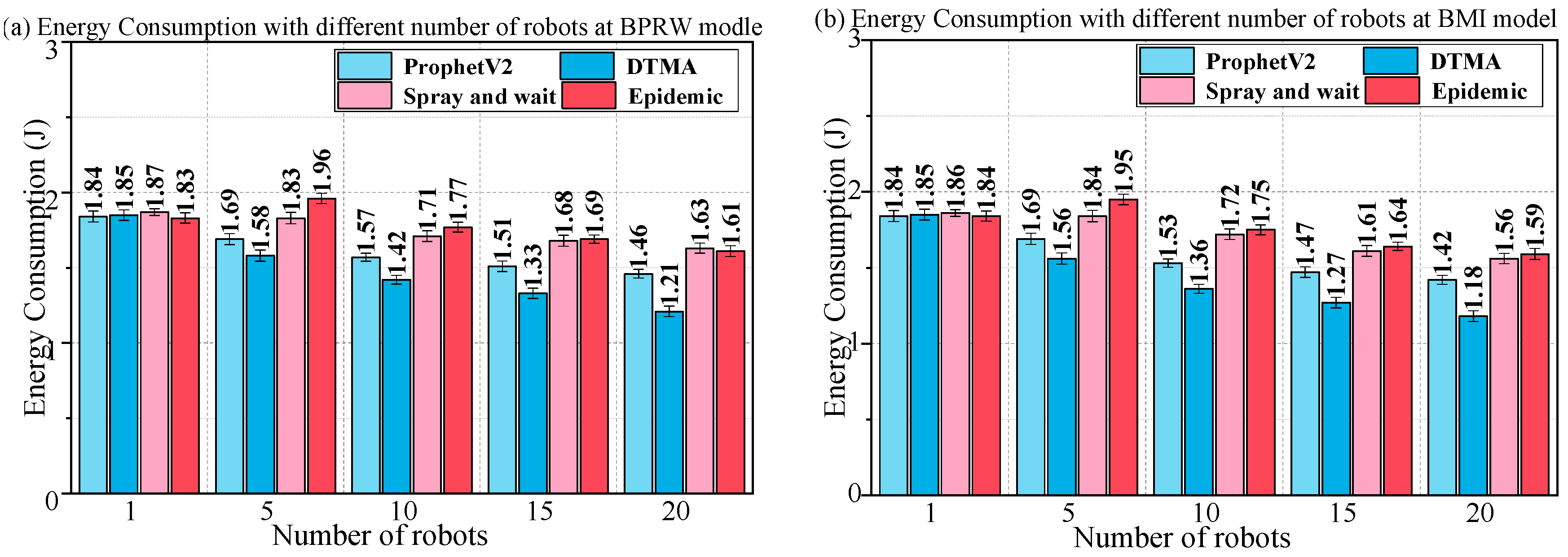
For Sub-scenarios 3.1–3.2, it can be seen from Figure 21, Figure 22, Figure 23, Figure 24, Figure 25 and Figure 26 that, all protocols have a similar performance with Scenario 2. The proposed DTMA performs best on the indexes of delivery ratio and energy consumption. Regarding hop count and overhead performance, Prophet V2 and Spray and Wait have the smallest number of hops and overheads, and DTMA almost performs the worst. Figure 22 also indicates that delay acts as a decreasing function of the rate of robots for all protocols. DTMA and Spray and Wait show the smallest delay as the rate increases, followed by Epidemic and Prophet V2. Finally, Prophet V2 and DTMA perform best on life time (Figure 26).
Figure 21, Figure 22, Figure 23, Figure 24, Figure 25 and Figure 26 show the difference in the performance of two motion models. It can be indicated that with the number of robots increasing, the difference between the performances of network under the two motion models becomes larger. When the number of robots is maintained at 1–5, the network performances under both models are approximately the same. After the number of robots increase to 10–20, all protocols have a better network performance when the robots follow uniform distribution in the map (BMI model). However, the performance of network life time is an exception (Figure 26). All protocols have a longer lifetime when robots can randomly move on the paths (BPRW model).
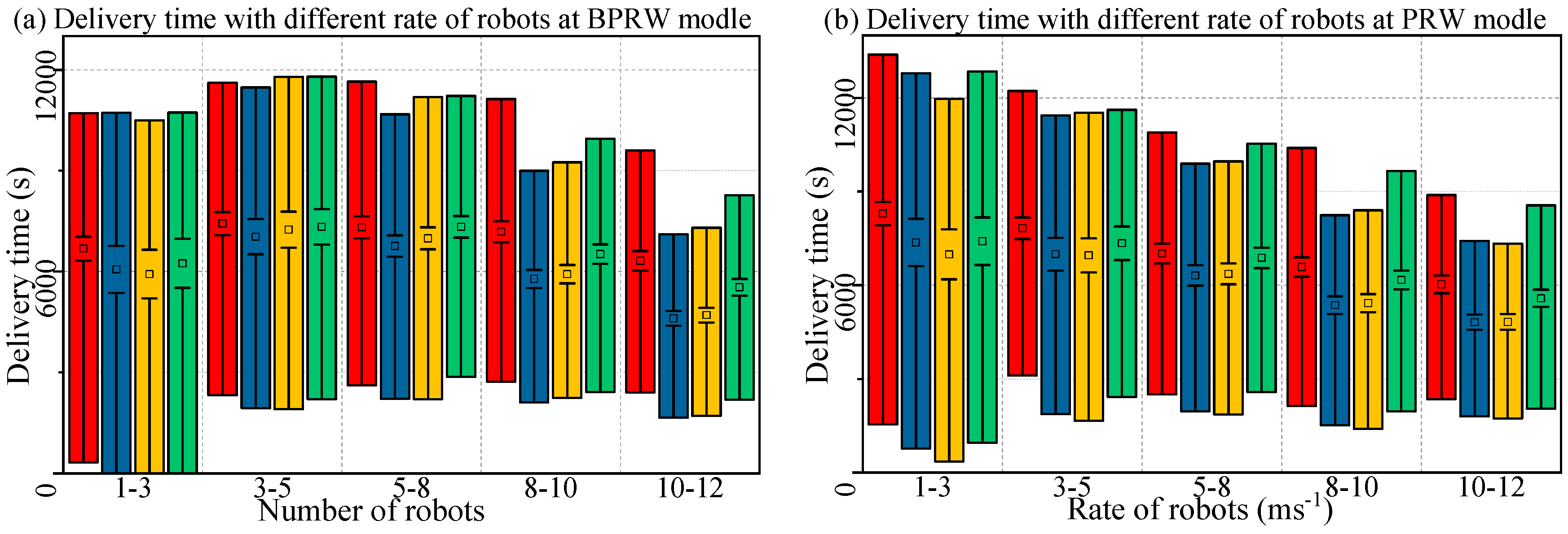
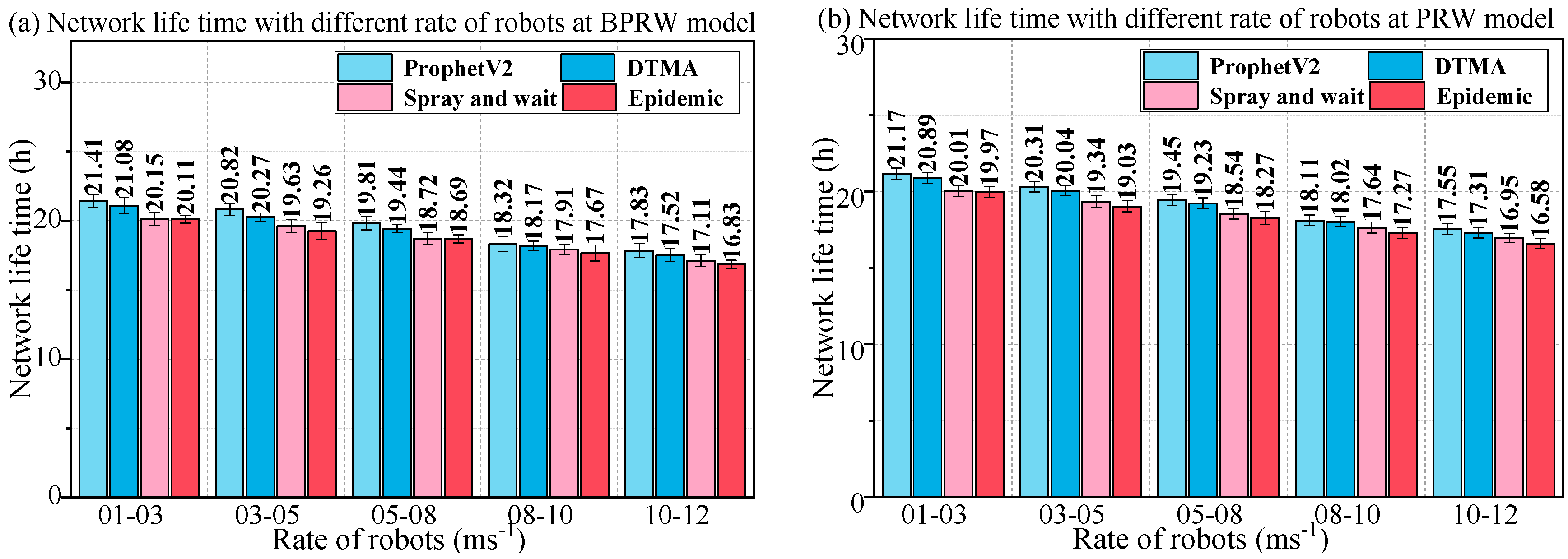
For Sub-scenarios 3.3–3.4, it can be seen from Figure 27, Figure 28, Figure 29, Figure 30, Figure 31 and Figure 32 that all protocols have a similar performance with Scenario 2. The proposed DTMA has the best performance on the delivery ratio and energy consumption. Regarding the hop count and the overhead performance, Prophet V2 and Spray and Wait have the smallest number of hops and overheads, and DTMA almost perform the worst. Figure 28 also indicates that the delay acts as a decreasing function of the rate of robots for all protocols. DTMA and Spray and Wait show the smallest delay as the rate increases, followed by Epidemic and Prophet V2. Finally, Prophet V2 and DTMA have the best life time performance (Figure 32).
Figure 27, Figure 28, Figure 29, Figure 30, Figure 31 and Figure 32 show the divergence in the performance of two motion models. In addition, it can be indicated that in most cases, all protocols have a better network performance when the robots follow one direction in the map (BPRW model). However, network life time performance is an exception (Figure 32). All protocols have a longer lifetime when robots can freely move on the path (PRW model).
4.5. Analysis and Verification of Results
In this paper, multiple RDTSN scenarios are performed for a transmission line monitoring system. All the obtained results have been analyzed and described in detail in this section. In addition, the simulation results have been verified by the field experiments of transmission line monitoring.
4.5.1. Analysis of Simulation Results
Simulation results are analyzed and discussed in this section. The analysis is divided into two parts, i.e., analysis of different routes in multiple scenarios and analysis of the effect of different motion models on network performance.
(1) Analysis of the change rules of routings with the different parameters
Adjusting transmission ranges or robot rate means changing the probability of node encounters. For all protocols, the message delivery ratio will increase as the nodes meet frequently. However, Prophet V2 performs the worst, as it is impossible to accurately describe the relationship among the network changes in RDTSN. As the large number of copies can clog the network, the growth of Epidemic’s delivery rate is also limited. Spray and Wait adopts the mechanism of restricting the number of copies, which determines its better performance in delivery ratio. The proposed DTMA considers the link availability that uses the calculation of the signal strength, which enhances the performance of message delivery. The best delivery performance is achieved in the simulation. The increase in the probability of node encounters also has a significant improvement in delivery time.
For all protocols, increasing buffer size can affect the update rate of messaging. In particular, an excessively small buffer size can significantly accelerate the message update rate, resulting in the discard of a large number of delayed messages. This process allows messages to be delivered in a real-time manner, as shown in Figure 18, where the values of message delay and delivery rate are both maintained at very low levels. When buffer size is large enough, such as over 500 M in Scenario 2, as shown in Figure 18, Figure 19 and Figure 20, since all message updates are not limited by buffer size, all policy performances tend to be stable. Under this situation, the performance of each algorithm is more dependent on the change in the probability of node encounters.
The change in the number of robots not only changes the probability of node encounters but also changes the total amount of messages. With the increase in the number of robots, the node interaction capability is strengthened, and the congestion of messages is increased. This results in a positive correlation between the delivery rate and the number of robots for all algorithms, and it also forms a stable delay. In addition, this phenomenon of stable delay can also be proved by the comparison of Figure 21, Figure 22, Figure 23, Figure 24, Figure 25 and Figure 26 and Figure 27, Figure 28, Figure 29, Figure 30, Figure 31 and Figure 32.
In the simulation, Epidemic and DTMA try to deliver more messages through more hops. Epidemic does not discriminate between the delivery of copies, resulting in the worst performance in energy consumption, and the increase in hops, copies and overhead. DTMA has good energy consumption performance in different scenarios. This is because it filters transmission paths by calculating energy consumption. However, due to the consideration of energy consumption, DTMA always tries to choose a short path with lower energy consumption, which also leads to an increase in the number of copies, hop count and overheads.
(2) Analysis of the effect of different motion models on network performance
Three motion models based on RDTSN are proposed. These models have different performances in dynamic scenarios. Firstly, PRW is a basic random motion model. Although PRW model is simple and has low cost of control, the network performance is not satisfying, especially in high-speed scenarios, where the probability of motion interference and uneven distribution is increased because of the random motion of the robot on a single ground line, and the performance of the PRW-based network is not satisfying. Secondly, BPRW model introduces a two-way traffic rule, which reduces the motion interference. Therefore, when the number of robots reaches 10–20, the performance of the network can be further improved due to the uneven distribution of the robots. Thirdly, BMI model integrates the advantages of BPRW model, and introduces a balanced distribution formation control. In multi-robot scenarios, BMI model improves the efficiency of multi-robot coordination and the network performance of RDTSN.
4.5.2. Verification of Simulation Results
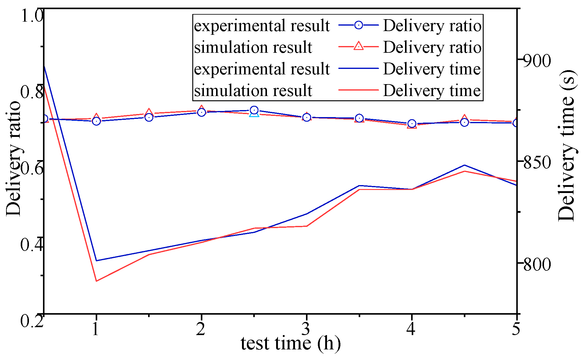
The effectiveness and reliability of RDTSN are verified by the field experiment and the results are shown in Figure 33. The field experiment is performed on an experimental transmission line with multi loops. In order to construct the experiment scenario, one WCN and two SNs are configured along the transmission line. There are two inspection robots walking on the experimental transmission line. A Mobile Monitoring Station (MMS) is set up as the CMP at 1000 m outside the experimental site.
DTMA is tested in a field experiment lasting 5 h. During the experiment, two robots are running on two ground wires respectively. The parameters of the test are shown in Table 9. In the process of experiment, MMS, robots and other nodes can establish effective communication with each other. The results of the experiment and the simulation are shown in Figure 34. The results of the field experiment are highly similar to those of simulation, which proves that the simulation can well reflect the performance of network and can act as a reference for comparison.
5. Discussion
The idea of RDTSN is derived from the rapid development and application of WSN technology, DTSN technology and robot technology. The most significant characteristic of RDTSN is wireless transmission of the inspection data by the inspection robots and the static nodes along a ground wire. Its communication mode is different from the real-time network with low delay and high cost of operation and maintenance. It is also different from Vehicle Delay-Tolerant Networks whose wireless signal could be frequently blocked by trees and buildings, etc. WSN and robot technologies have been rapidly developing in recent years, especially in terms of the light weight and cost-effectiveness of hardware. Thus, it becomes possible to build a WSN with a robot as the core node and propose a new method for monitoring high-voltage lines. RDTSN, combining the characteristics of WSN, Robot and DTSN, is very distinctive network. Firstly, the network structure is changeable and flexible for mobile robots as the intermediate transmission point of information; secondly, the network has the properties of delay-tolerance and intermittent connectivity; thirdly, as fewer nodes are deployed, the deployment costs are decreased, and the fault-tolerant performance is improved. These characteristics of RDTSN provide a strong technological support for the security of inspection data.
The main contribution of the proposed method is to enhance the intelligent level of power grid monitoring system and the data transmission quality of patrolling line. At present, the robot mainly uses the point-to-point communication mode when it is inspecting the transmission line. That is, a robot can only communicate with one MMS. Thus, such a communication mode seriously restricts the large-scale application of robotic line inspection. In this paper, a highly practical robot delay-tolerant sensor network (RDTSN) is proposed, which greatly reduces the workload of operators and improves the intelligence level of the transmission line inspection. Further, this research makes a new attempt in theory: The motion model of the inspection robot is analyzed and summed up, and the delivery rate and energy consumption factor are introduced for the mathematical modeling of RDTSN. Under the premise of guaranteeing the message delivery rate, the energy consumption of the node is reduced and the network life is extended. Finally, we design the routing algorithm (DTMA) based on the mathematical model, which balances the relationship between the delivery rate and the energy consumption, compares and chooses the optimized destination of the message, which greatly improves the reliability and practicability of the network. In addition, this can be seen from the simulation result.
The proposed method also needs improvement in several aspects in practical applications. Firstly, the RDTSN’s data has a high delay—as the result is shown in Section 4 there are over 60 min delay in general—and it is difficult to alarm the line burst fault in timely manner. This means the monitoring network can only do routine inspection and a lagged processing of the fault point. In addition, RDTSN is not compared with other methodologies and telecommunications technologies such as LPWAN (Low-Power Wide-Area Network). A more reasonable method combines LPWAN, and other technologies are going to be adopted to improve delivery time and energy consumption. Secondly, the adaptive adjustment of network message delivery and energy consumption cannot be realized currently. The energy factor in the method needs to be preset, as we did in Section 4.2. An intelligent algorithm, such as the deep learning method, can be possibly introduced to realize the adaptive adjustment of energy factor. Thirdly, the RDTSN-optimized routing algorithm (DTMA) reduces network energy consumption under the premise of ensuring a better message delivery rate. However, it also increases the network overheads and hop count, and it is almost the worst one in the simulation results. It means that the efficiency of routing algorithm needs to be improved. A more reasonable way is going to be adopted to limit the number of message copies to improve the efficiency of the algorithm.
6. Conclusions
This paper proposes a novel method of wireless monitoring system for transmission lines using RDTSN. The main conclusions are summarized as follows:
- (1)
- RDTSN is able to act as a new type of intelligent monitoring system to automatically inspect transmission lines. Because the robot always moves along the ground wire, the inspection data can be collected by the other nodes and forwarded to CMP for analysis. In addition, all the nodes of the RDTSN are in the air, without the wireless signal blocked by trees and buildings, and with an excellent adaptability. As a small number of robots are replaced with a large number of static nodes, the availability and the economy of the monitoring systems have been improved.
- (2)
- The proposed method mainly includes two parts, the RDTSN model and the data delivery strategy. In the first part, the composition and structure of the network are introduced. Then, the characteristics of the robot motion are analyzed, and two new motion models are proposed. Finally, a new mathematical model for the network is proposed. The proposed model fully considers the characteristics of the transmission lines and robots, and a scheme is designed to balance the message delivery rate and the network energy consumption. In the next part, a new routing algorithm (DTMA) is designed. DTMA is similar to the prophet algorithm, where the social information is used to calculate the link availability probability. Then, the mathematical model is combined to update the weight of the links. Finally, the homogeneous destinations of RDTSN are ranked.
- (3)
- In simulation experiments, three experimental scenarios performed including six network targets. Experimental results show that the RDTSN can complete the effective transmission of inspection data using the proposed DTMA and other three routing protocols, which verifies the effectiveness of the proposed method. In the comparison experiment, the proposed DTMA can perform as well as the other routing protocols in most cases or even better in some respects, such as the delivery ratio and the energy consumption, which verifies the feasibility of the proposed method.
Further research should mainly focus on the following aspects. One is that it is more difficult to set the effective thresholds of RDTSN if the change trends of network performances are not obvious. The network mathematical model should be further improved to obtain better self-adaptive ability of energy consumption. The other is that DTMA sometimes cannot achieve ideal overheads and hop count in simulations. A multi-factor analysis needs to be performed on the control of the replication and forwarding of messages. It is noteworthy that all wireless nodes use IEEE 802.11n as the communication protocol in the simulation and field experiments of this paper. Although it provides a high data rate, it has a great energy consumption. In subsequent studies, we will try to use similar IEEE 802.15.4 protocol to obtain a lower energy consumption. In addition, we are ready to use RDTSN and DTMA for real tests in the actual scenarios (the scenarios simulated in this paper).
Author Contributions
F.F. proposed and developed the research design, designed the simulation experiment, collected the experimental data, performed the data analysis, results interpretation and manuscript writing. G.W. assisted with developing the research design and results interpretation. M.W. assisted with refining the manuscript writing and coordinating the revision activities. Q.C. and S.Y. assisted with process of experiments.
Acknowledgments
This work was supported by a Guangdong Robot Special Project (2015B090922007), a Foshan Technical Innovation Team Project (2015IT100143), a National Science and Technology Major Project (2014ZX04015021), and a State Grid Jilin Electric Power Co., Ltd. Project, China (JDK2015-21). The authors also wish to thank anonymous reviewers, each of whom provided comments that directed important improvements in the manuscript.
Conflicts of Interest
The authors declare no conflict of interest.
References
- Machowski, J.; Bialek, J.; Bumby, J. Power System Dynamics: Stability and Control; John Wiley & Sons: New York, NY, USA, 2009; pp. 29–30. [Google Scholar]
- Mazur, K.; Wydra, M.; Ksiezopolski, B. Secure and Time-Aware Communication of Wireless Sensors Monitoring Overhead Transmission Lines. Sensors 2017, 17, 1610. [Google Scholar] [CrossRef] [PubMed]
- Wu, Y.C.; Cheung, L.F.; Lui, K.S.; Pong, P.W.T. Efficient Communication of Sensors Monitoring Overhead Transmission Lines. IEEE Trans. Smart Grid 2012, 3, 1130–1136. [Google Scholar] [CrossRef] [Green Version]
- Miller, R.; Abbasi, F.; Mohammadpour, J. Power line robotic device for overhead line inspection and maintenance. Ind. Robot 2017, 44, 75–84. [Google Scholar] [CrossRef]
- Lazaropoulos, A.G. Wireless Sensor Network Design for Transmission Line Monitoring, Metering, and Controlling: Introducing Broadband over power lines-enhanced network model (BPLeNM). ISRN Power Eng. 2014, 2014. [Google Scholar] [CrossRef]
- Qin, X.; Wu, G.; Lei, J.; Fan, F. A Novel Method of Autonomous Inspection for Transmission Line based on Cable Inspection Robot LiDAR Data. Sensors 2018, 18, 596. [Google Scholar] [CrossRef] [PubMed]
- Jiang, W.; Wu, G.; Fan, F. Autonomous location control of a robot manipulator for live maintenance of high-voltage transmission lines. Ind. Robot 2017, 44, 671–686. [Google Scholar] [CrossRef]
- Kim, J.; Kim, D.; Lim, K.W.; Ko, Y.B.; Lee, S.Y. Improving the reliability of IEEE 802.11 s based wireless mesh networks for smart grid systems. J. Commun. Netw. 2012, 14, 629–639. [Google Scholar] [CrossRef]
- Moghe, R.; Lambert, F.C.; Divan, D. Smart “stick-on” sensors for the smart grid. IEEE Trans. Smart Grid 2012, 3, 241–252. [Google Scholar] [CrossRef]
- Fateh, B.; Govindarasu, M.; Ajjarapu, V. Wireless Network Design for Transmission Line Monitoring in Smart Grid. IEEE Trans. Smart Grid 2013, 4, 1076–1086. [Google Scholar] [CrossRef]
- Rusinek, D.; Ksiezopolski, B.; Wierzbicki, A. Security Trade-Off and Energy Efficiency Analysis in Wireless Sensor Networks. IJDSN 2015, 11, 943475:1–943475:17. [Google Scholar] [CrossRef]
- Khabbaz, M.J.; Assi, C.M.; Fawaz, W.F. Disruption-tolerant networking: A comprehensive survey on recent developments and persisting challenges. IEEE Commun. Surv. Tutor. 2012, 14, 607–640. [Google Scholar] [CrossRef]
- Gomez, C.; Paradells, J. Urban Automation Networks: Current and Emerging Solutions for Sensed Data Collection and Actuation in Smart Cities. Sensors 2015, 15, 22874–22898. [Google Scholar] [CrossRef] [PubMed] [Green Version]
- Velásquez-Villada, C.; Solano, F.; Donoso, Y. Routing Optimization for Delay Tolerant Networks in Rural Applications Using a Distributed Algorithm. Int. J. Comput. Commun. Control 2014, 10, 100–111. [Google Scholar] [CrossRef]
- Wang, C.; Guo, S.; Yang, Y. An Optimization Framework for Mobile Data Collection in Energy-Harvesting Wireless Sensor Networks. IEEE Trans. Mob. Comput. 2016, 12, 2969–2986. [Google Scholar] [CrossRef]
- Project Loon. Google Inc. Available online: https://www.google.com/loon/ (accessed on 18 February 2016).
- Internet.org. Facebook Inc. Available online: https://www.internet.org/projects (accessed on 18 February 2016).
- Raffelsberger, C.; Hellwagner, H. A hybrid MANET-DTN routing scheme for emergency response scenarios. In Proceedings of the IEEE International Conference on Pervasive Computing and Communications Workshops IEEE Computer Society, San Diego, CA, USA, 18–22 March 2013; pp. 505–510. [Google Scholar]
- Asuquo, P.; Cruickshank, H.; Sun, Z.; Chandrasekaran, G. Analysis of DoS Attacks in Delay Tolerant Networks for Emergency Evacuation. In Proceedings of the International Conference on Next Generation Mobile Applications, Services and Technologies, Cambridge, UK, 9–11 September 2015; pp. 228–233. [Google Scholar]
- Jiang, P.; Bigham, J.; Bodanese, E. Adaptive service provisioning for emergency communications with DTN. In Proceedings of the Wireless Communications and Networking Conference, Quintana Roo, Mexico, 28–31 March 2011; pp. 2125–2130. [Google Scholar]
- Pentland, A.; Fletcher, R.; Hasson, A. Daknet: Rethinking connectivity in developing nations. Computer 2004, 37, 78–83. [Google Scholar] [CrossRef]
- Zhang, Y.; Liang, J.; Jiang, S. A Localization Method for Underwater Wireless Sensor Networks Based on Mobility Prediction and Particle Swarm Optimization Algorithms. Sensors 2016, 16, 212. [Google Scholar] [CrossRef] [PubMed]
- Kim, H.; Cho, H.S. SOUNET: Self-Organized Underwater Wireless Sensor Network. Sensors 2017, 17, 283. [Google Scholar] [CrossRef] [PubMed]
- Wang, Y.; Wu, H. Delay/fault-tolerant mobile sensor network (DFT-MSN): A new paradigm for pervasive information gathering. IEEE Trans. Mob. Comput. 2006, 6, 1021–1034. [Google Scholar] [CrossRef]
- Vahdat, A.; Becker, D. Epidemic Routing for Partially Connected Ad Hoc Networks; Technical Report CS-200006; Duke University: Durham, NC, USA, 2000. [Google Scholar]
- Spyropoulos, T.; Psounis, K.; Raghavendra, C.S. Spray and Wait: An Efficient Routing Scheme for Intermittently Connected Mobile Networks. In Proceedings of the 2005 ACM SIGCOMM Workshop on Delay-Tolerant Networking, Philadelphia, PA, USA, 22–26 August 2005. [Google Scholar]
- Lindgren, A.; Doria, A.; Davies, E.; Grasic, S. Probabilistic Routing Protocol for Intermittently Connected Networks. Available online: https://tools.ietf.org/html/rfc6693 (accessed on 13 March 2016).
- Hui, P.; Crowcroft, J.; Yoneki, E. BUBBLE Rap: Social-based Forwarding in Delay Tolerant Networks. In Proceedings of the ACM MobiHoc’08, Hong Kong, China, 26–30 May 2008. [Google Scholar]
- Daly, E.M.; Haahr, M. Social network analysis for routing in disconnected delay-tolerant manets. In Proceedings of the ACM MobiHoc’07, Montreal, QC, Canada, 9–14 September 2007. [Google Scholar]
- Mtibaa, A.; May, M.; Diot, C.; Ammar, M. Peoplerank: Social opportunistic forwarding. In Proceedings of the IEEE INFOCOM’10, San Diego, CA, USA, 15–19 March 2010. [Google Scholar]
- Yasmine, D.; Bouabdellah, K.; Mohammed, F. Using Mobile Data Collectors to Enhance Energy Efficiency and Reliability in Delay Tolerant Wireless Sensor Networks. J. Inf. Process. Syst. 2016, 12, 275–294. [Google Scholar]
- Velásquez-Villada, C.; Donoso, Y. Delay/Disruption Tolerant Network-Based Message Forwarding for a River Pollution Monitoring Wireless Sensor Network Application. Sensors 2016, 16, 436. [Google Scholar] [CrossRef] [PubMed]
- Keränen, A.; Ott, J.; Kärkkäinen, T. The ONE Simulator for DTN Protocol Evaluation. In Proceedings of the 2nd International Conference on Simulation Tools and Techniques (ICST), Rome, Italy, 2–6 March 2009. [Google Scholar]
- Graf, F.; Kriegel, H.P.; Renz, M. MARiO: Multi-Attribute Routing in Open Street Map. Advances in Spatial and Temporal Databases; Springer: Berlin/Heidelberg, Germany, 2011; pp. 486–490. [Google Scholar]
Figure 1.
Inspection robot project running in Jilin, 2016–2017. (a) Power tower and additional device; (b) Inspection robot; (c) Mobile Monitoring Station (MMS).
Figure 1.
Inspection robot project running in Jilin, 2016–2017. (a) Power tower and additional device; (b) Inspection robot; (c) Mobile Monitoring Station (MMS).

Figure 2.
Research directions of DTSN.

Figure 3.
Robot Delay-Tolerant Sensor Network (RDTSN). OPGW, Optical Fiber Composite Overhead Ground Wire.
Figure 3.
Robot Delay-Tolerant Sensor Network (RDTSN). OPGW, Optical Fiber Composite Overhead Ground Wire.

Figure 4.
Tow movement models of robot. (a) PRW movement model; (b) BPRW movement model.

Figure 5.
BMI movement models of robot. (a) State one; (b) state two.

Figure 6.
Network representation. (a) Two-node graph; (b) five-node graph.

Figure 7.
Network extended graph with the availability weights through time represented at once.

Figure 8.
Network routing solution.

Figure 9.
RDTSN scenarios map. (a) Scenarios map from Open Street Map; (b) simulation interface of the RDTSN in the ONE (Opportunistic Network Environment) simulator.
Figure 9.
RDTSN scenarios map. (a) Scenarios map from Open Street Map; (b) simulation interface of the RDTSN in the ONE (Opportunistic Network Environment) simulator.

Figure 10.
Results of the scenario of default value, delivery time and distance at message send and hop count.
Figure 10.
Results of the scenario of default value, delivery time and distance at message send and hop count.

Figure 11.
Statistical analysis data of delivery time and distance at message send and hop count, the blue scatter point is the result of data distribution, the red histogram is the statistical result of the data distribution.
Figure 11.
Statistical analysis data of delivery time and distance at message send and hop count, the blue scatter point is the result of data distribution, the red histogram is the statistical result of the data distribution.

Figure 12.
Results of Scenario 1 of DTMA. (a) Delivery ratio, network life time and hop count with different alpha in Scenario 1.1–1.3; (b) delivery ratio, network life time and hop count with different alpha in Scenario 1.4–1.5.
Figure 12.
Results of Scenario 1 of DTMA. (a) Delivery ratio, network life time and hop count with different alpha in Scenario 1.1–1.3; (b) delivery ratio, network life time and hop count with different alpha in Scenario 1.4–1.5.

Figure 13.
Results of Scenario 1 of Prophet V2. (a) Delivery ratio, delivery time with different beta in Scenario 1.1–1.3; (b) delivery ratio, deliver time with different beta in Scenario 1.4–1.5.
Figure 13.
Results of Scenario 1 of Prophet V2. (a) Delivery ratio, delivery time with different beta in Scenario 1.1–1.3; (b) delivery ratio, deliver time with different beta in Scenario 1.4–1.5.

Figure 14.
Results of Scenario 1 of Spray and Wait. (a) Delivery ratio, delivery time with different number of copies in Scenario 1.1–1.3; (b) delivery ratio, deliver time with different number of copies in Scenario 1.4–1.5.
Figure 14.
Results of Scenario 1 of Spray and Wait. (a) Delivery ratio, delivery time with different number of copies in Scenario 1.1–1.3; (b) delivery ratio, deliver time with different number of copies in Scenario 1.4–1.5.

Figure 15.
Results of Scenario 2.1. (a) Delivery ratio with different transmission ranges of nodes; (b) delivery time in seconds with different transmission ranges of nodes.
Figure 15.
Results of Scenario 2.1. (a) Delivery ratio with different transmission ranges of nodes; (b) delivery time in seconds with different transmission ranges of nodes.

Figure 16.
Results of Scenario 2.1. (a) Overheads with different transmission ranges of nodes; (b) hop count with different transmission ranges of nodes.
Figure 16.
Results of Scenario 2.1. (a) Overheads with different transmission ranges of nodes; (b) hop count with different transmission ranges of nodes.

Figure 17.
Results of Scenario 2.1. (a) Network life time with different transmission ranges of nodes; (b) energy consumption with different transmission ranges of nodes.
Figure 17.
Results of Scenario 2.1. (a) Network life time with different transmission ranges of nodes; (b) energy consumption with different transmission ranges of nodes.

Figure 18.
Results of Scenario 2.2. (a) Delivery ratio with different buffer sizes; (b) delivery time in seconds with different buffer sizes.
Figure 18.
Results of Scenario 2.2. (a) Delivery ratio with different buffer sizes; (b) delivery time in seconds with different buffer sizes.

Figure 19.
Results of Scenario 2.2. (a) Overheats with different buffer sizes; (b) hop count with different buffer sizes.
Figure 19.
Results of Scenario 2.2. (a) Overheats with different buffer sizes; (b) hop count with different buffer sizes.

Figure 20.
Results of Scenario 2.2. (a) Network life time with different number of robots; (b) energy consumption with different number of robots.
Figure 20.
Results of Scenario 2.2. (a) Network life time with different number of robots; (b) energy consumption with different number of robots.

Figure 21.
Results of Scenario 3, Delivery ratio with different number of robots. (a) BPRW movement model; (b) BMI movement model.
Figure 21.
Results of Scenario 3, Delivery ratio with different number of robots. (a) BPRW movement model; (b) BMI movement model.

Figure 22.
Results of Scenario 3, Delivery time with different number of robots. (a) BPRW movement model; (b) BMI movement model.
Figure 22.
Results of Scenario 3, Delivery time with different number of robots. (a) BPRW movement model; (b) BMI movement model.

Figure 23.
Results of Scenario 3, Overheads with different number of robots. (a) BPRW movement model; (b) BMI movement model.
Figure 23.
Results of Scenario 3, Overheads with different number of robots. (a) BPRW movement model; (b) BMI movement model.

Figure 24.
Results of Scenario 3, Hop count with different number of robots. (a) BPRW movement model; (b) BMI movement model.
Figure 24.
Results of Scenario 3, Hop count with different number of robots. (a) BPRW movement model; (b) BMI movement model.

Figure 25.
Results of Scenario 3, Network life time with different number of robots. (a) BPRW movement model; (b) BMI movement model.
Figure 25.
Results of Scenario 3, Network life time with different number of robots. (a) BPRW movement model; (b) BMI movement model.

Figure 26.
Results of Scenario 3, Energy consumption with different number of robots. (a) BPRW movement model; (b) BMI movement model.
Figure 26.
Results of Scenario 3, Energy consumption with different number of robots. (a) BPRW movement model; (b) BMI movement model.

Figure 27.
Results of Scenario 3, Delivery ratio with different rate of robots. (a) BPRW movement model; (b) PRW movement model.
Figure 27.
Results of Scenario 3, Delivery ratio with different rate of robots. (a) BPRW movement model; (b) PRW movement model.

Figure 28.
Results of Scenario 3, Delivery time with different rate of robots. (a) BPRW movement model; (b) PRW movement model.
Figure 28.
Results of Scenario 3, Delivery time with different rate of robots. (a) BPRW movement model; (b) PRW movement model.

Figure 29.
Results of Scenario 3, Overheads with different rate of robots. (a) BPRW movement model; (b) PRW movement model.
Figure 29.
Results of Scenario 3, Overheads with different rate of robots. (a) BPRW movement model; (b) PRW movement model.

Figure 30.
Results of Scenario 3, Hop count with different rate of robots. (a) BPRW movement model; (b) PRW movement model.
Figure 30.
Results of Scenario 3, Hop count with different rate of robots. (a) BPRW movement model; (b) PRW movement model.

Figure 31.
Results of Scenario 3, Network life time with different rate of robots. (a) BPRW movement model; (b) PRW movement model.
Figure 31.
Results of Scenario 3, Network life time with different rate of robots. (a) BPRW movement model; (b) PRW movement model.

Figure 32.
Results of Scenario 3, Energy consumption with different rate of robots. (a) BPRW movement model; (b) PRW movement model.
Figure 32.
Results of Scenario 3, Energy consumption with different rate of robots. (a) BPRW movement model; (b) PRW movement model.

Figure 33.
The field experiments. (a) Robot and static node; (b) MMS, communication device and antenna.
Figure 33.
The field experiments. (a) Robot and static node; (b) MMS, communication device and antenna.

Figure 34.
Result of field experiments and simulations.


Table 1.
Default parameters of the simulation.
| Parameter | Default Value |
|---|---|
| Network area size (m × m) | 74,500 × 143,400 |
| Simulation run time (s) | 86,400 |
| Number of Robots | 5 nodes |
| Number of SNs | 7 nodes |
| Number of WCNs | 5 nodes |
| RC (m) | 10,000 |
| RS (m) | 3000 |
| Movement rate of Robot (m/s) | 3–5 |
| Tpause (s) | 10–30 |
| Buffer size (M) | 500 |
| Message size (Kb) | 2000 |
| Robot message interval (s) | 60, 120 |
| SNs message interval (s) | 1800, 3600 |
| Source nodes | Robot, SNs |
| Destination nodes | WCNs |
| Movement model | BPRW |
| Alpha and Beta of DTMA | 0.78, 0.22 |
| Beta of Prophet V2 | 0.36 |
| Spray and Wait Router Copies | 8 |
Table 2.
Parameters of Scenario 1.
| Parameter | Scenario 1.1 | Scenario 1.2 | Scenario 1.3 | Scenario 1.4 | Scenario 1.5 |
|---|---|---|---|---|---|
| Numbers of robots | 1 | 5 | 10 | 5 | 5 |
| Movement rate (ms−1) | 3–5 | 3–5 | 3–5 | 1–3 | 5–8 |
Table 3.
Parameters of Scenario 2.1.
| Parameter (km) | Rs1, Rc1 | Rs2, Rc2 | Rs3, Rc3 | Rs4, Rc4 | Rs5, Rc5 |
|---|---|---|---|---|---|
| Transmission range | 1, 3 | 2, 6.5 | 3, 10 | 4, 13 | 5, 17 |
Table 4.
Parameters of Scenario 2.2.
| Parameter (M) | Buffer 1 | Buffer 2 | Buffer 3 | Buffer 4 | Buffer 5 | Buffer 6 | Buffer 7 |
|---|---|---|---|---|---|---|---|
| Buffer size | 5 | 10 | 20 | 50 | 200 | 500 | 1000 |
Table 5.
Parameters of Scenario 3.1.
| Parameter | Motion 1 | Motion 2 | Motion 3 | Motion 4 | Motion 5 |
|---|---|---|---|---|---|
| Number of robots | 1 | 5 | 10 | 15 | 20 |
| Movement model | BPRW | BPRW | BPRW | BPRW | BPRW |
Table 6.
Parameters of Scenario 3.2.
| Parameter | Motion 1 | Motion 2 | Motion 3 | Motion 4 | Motion 5 |
|---|---|---|---|---|---|
| Number of robots | 1 | 5 | 10 | 15 | 20 |
| Movement model | BMI | BMI | BMI | BMI | BMI |
Table 7.
Parameters of Scenario 3.3.
| Parameter (m/s) | Motion 1 | Motion 2 | Motion 3 | Motion 4 | Motion 5 |
|---|---|---|---|---|---|
| Movement rate | 1–3 | 3–5 | 5–8 | 8–10 | 10–12 |
| Movement model | BPRW | BPRW | BPRW | BPRW | BPRW |
Table 8.
Parameters of Scenario 3.4.
| Parameter (m/s) | Motion 1 | Motion 2 | Motion 3 | Motion 4 | Motion 5 |
|---|---|---|---|---|---|
| Movement rate | 1–3 | 3–5 | 5–8 | 8–10 | 10–12 |
| Movement model | PRW | PRW | PRW | PRW | PRW |
Table 9.
Default parameters of field experiment.
| Parameter | Default Value |
|---|---|
| Network area size (m × m) | 1000 × 15,000 |
| Test time (h) | 5 |
| Number of Robots | 2 nodes |
| Number of SNs | 2 nodes |
| Number of WCNs | 1 nodes |
| RC (m) | 3000 |
| RS (m) | 1000 |
| Movement rate of Robot (m/s) | 3–5 |
| Tpause (s) | 10–30 |
| Buffer size (M) | 500 |
| Message size (Kb) | 2000 |
| Robot message interval (s) | 60, 120 |
| SNs message interval (s) | 1800, 3600 |
| Source nodes | Robot, SNs |
| Destination nodes | MMS |
| Movement model | BPRW |
| Alpha and Beta of DTMA | 0.71, 0.29 |
© 2018 by the authors. Licensee MDPI, Basel, Switzerland. This article is an open access article distributed under the terms and conditions of the Creative Commons Attribution (CC BY) license (http://creativecommons.org/licenses/by/4.0/).
Share and Cite
MDPI and ACS Style
Fan, F.; WU, G.; Wang, M.; Cao, Q.; Yang, S. Robot Delay-Tolerant Sensor Network for Overhead Transmission Line Monitoring. Appl. Sci. 2018, 8, 847. https://doi.org/10.3390/app8060847
AMA Style
Fan F, WU G, Wang M, Cao Q, Yang S. Robot Delay-Tolerant Sensor Network for Overhead Transmission Line Monitoring. Applied Sciences. 2018; 8(6):847. https://doi.org/10.3390/app8060847
Chicago/Turabian StyleFan, Fei, Gongping WU, Man Wang, Qi Cao, and Song Yang. 2018. "Robot Delay-Tolerant Sensor Network for Overhead Transmission Line Monitoring" Applied Sciences 8, no. 6: 847. https://doi.org/10.3390/app8060847
Note that from the first issue of 2016, this journal uses article numbers instead of page numbers. See further details here.