Review on Structural Health Evaluation with Acoustic Emission


Department of Materials Science and Engineering, University of California, Los Angeles (UCLA), Los Angeles, CA 90095, USA
Appl. Sci. 2018, 8(6), 958; https://doi.org/10.3390/app8060958
Submission received: 20 May 2018
/
Revised: 7 June 2018
/
Accepted: 8 June 2018
/
Published: 11 June 2018
(This article belongs to the Special Issue Structural Health Monitoring of Large Structures Using Acoustic Emission–Case Histories)
Abstract
:This review introduces several areas of importance in acoustic emission (AE) technology, starting from signal attenuation. Signal loss is a critical issue in any large-scale AE monitoring, but few systematic studies have appeared. Information on damping and attenuation has been gathered from metal, polymer, and composite fields to provide a useful method for AE monitoring. This is followed by discussion on source location, bridge monitoring, sensing and signal processing, and pressure vessels and tanks, then special applications are briefly covered. Here, useful information and valuable sources are identified with short comments indicating their significance. It is hoped that readers note developments in areas outside of their own specialty for possible cross-fertilization.
1. Introduction
Nondestructive evaluation (NDE) of various structures, large and small, has been the primary target of acoustic emission (AE) technology along with its uses in materials research. The first success of AE technology was achieved at Aerojet for the inspection of Polaris missile chambers in the 1960s [1]. Further works continued for nuclear and chemical pressure vessels and tanks [2,3]. For industrial AE applications to fiber reinforced plastics (FRP) vessels, the Committee on Acoustic Emission for Reinforced Plastics (CARP) was instrumental in code development, culminating in ASME Boiler and Pressure Vessels Codes and ASTM standards. See Fowler et al. [4] and four following articles in the special issue of Journal of AE in 1989. A wide range of AE applications have been compiled in the AE volume of the Nondestructive Testing Handbook [5], while many articles appeared in conference proceedings and in Journal of AE [6]. Shiotani [7] and Bohse [8] reviewed various applications of AE to infrastructures and to structural diagnosis, respectively. Two recent review articles [9,10] on bridge and pressure-vessel inspection are noteworthy in connection to the topic of this introduction. Another review was published as a Sandia report, comparing AE with other methods for structural health monitoring (SHM) in evaluating damages to a full-scale wind turbine blade, and demonstrating the advantages of AE over others [11]. The present author also prepared survey papers on structural diagnosis [12] and on composites [13]. A comprehensive monograph by Giurgiutiu [14] on SHM of aerospace composites appeared recently and AE monitoring for SHM was covered in depth. AE uses in SHM have fully integrated acousto-ultrasonic methods, taking advantage of piezoelectric wafer active sensors (PWAS). A review paper by Mitra [15] covering the roles of guided waves in SHM is also useful. With the wealth of these available resources, this article will focus on those topics not addressed adequately elsewhere.
2. Signal Attenuation
An important issue during any structural inspection using AE methods is the decrease in signal intensity or attenuation. On the AE side, signal-to-noise ratio is important in signal detection. In SHM applications, quantitative system modeling is often desired and attenuation behavior needs to be a part of successful SHM system design [16]. The same phenomena at lower frequencies are referred to as structural damping and a recent review relative to composite materials [17] provides useful backgrounds. This topic is also indirectly related to the mechanical properties of polymers since most polymers exhibit viscoelastic behavior and strong acoustic damping [18,19].
2.1. Guided Wave Attenuation
In using AE to examine structures, we typically deal with two-dimensional wave propagation since thick-walled structures—like nuclear pressure vessels and concrete dams—are exceptional cases. For theoretical developments and early experimental results, see Viktorov’s book from 1967 [20] or numerous other books that followed dealing with wave propagation, e.g., Rose [21]. In most instances, AE signals propagate along the surface as Rayleigh waves or through thin-walled structures as Lamb waves. These waves are collectively known as guided waves. When they spread on two-dimensional structures, signal loss occurs from geometrical spreading (with inverse square root dependence on travel distance, x, or 1/√x dependence). Additionally, attenuation is caused from material absorption and scattering with exponential decay, or exp(−x) with attenuation coefficient . Combined, signal amplitude decreases following (1/√x)·exp(−x). For dispersive Lamb waves, signal loss also arises from dispersion or frequency-dependent wave speed, which spreads vibration energy over a longer period, reducing signal amplitude [13,20]. When the surfaces are covered with liquids or other damping matters, attenuation occurs from vibration energy leakage. These appear as additional values. Mal et al. [22] gave an extension of wave propagation theory to anisotropic plates with dissipation given in terms of quality factors, Q. They presented several examples of attenuation in fiber reinforced composite plates.
Press and Healy [23] in 1957 gave theory and experimental confirmation for Rayleigh wave attenuation. Measured Rayleigh attenuation coefficients (R) for PMMA were nearly linear with frequency and was 55 dB/m at 100 kHz. Viktorov [20] provided a parametric equation for R and listed three more R values for aluminum (Dural or 2017 alloy), glass and polystyrene (15.4, 73.7, 422 dB/m at 1 MHz, respectively). In 1964, Zhukov et al. [24] derived theoretical expressions for Lamb wave attenuation coefficients, L. These guided wave attenuation coefficients, R and L, depend on the attenuation coefficients of longitudinal and transverse bulk waves, or p and t. Zhukov et al. [24] also measured L values for the 0th and 1st symmetric and asymmetric modes, or S0, S1, A0, and A1 modes on low carbon steel plates (C = 0.15%). The measured L values ranged from 3.8 to 5.7 dB/m at 1.3 MHz and were comparable to their longitudinal and shear wave attenuation coefficients, p = 3.7 and t = 3.9 dB/m. At zero thickness limit for S0, L = √2 t. Pressure-vessel and pipeline steels are known for their low bulk wave attenuation of p = 1 to 10 dB/m at 2 MHz as tabulated in Krautkramer’s book [25], which are reduced further at lower frequencies. Such low attenuation values for Al and steels below 10 dB/m were reported by Mason and McSkimin [26], Roderick and Truell [27], Kamigaki [28], and Papadakis [29,30] among others at frequencies up to 20 MHz. These data were obtained using directly bonded, low-loss quartz transducers. Some of these tests also included t measurements. Thus, guided waves are expected to propagate with low loss when materials possess low p values.
Wave attenuation is characterized using several different parameters. In the ultrasonic and AE fields, attenuation coefficient is commonly used to represent an exponential decay. We use two units for One is dB/m and the other Np/m with 8.686 dB = 1 Np. Np stands for Nepers, a non-dimensional unit, and is useful in numerical computation. This is also related to damping (or loss) factor η by η = λ/π, where λ is the wave length. Here, η is the ratio of energy dissipated per cycle to maximum energy stored per cycle, and is also equal to loss tangent, tan δ. This tan δ is defined as the ratio of imaginary part (E”) to real part (E’) of a complex modulus, E* = E’ − iE” with i2 = −1. The damping factor (or loss tangent) is often used in dealing with vibration damping at lower frequencies. Another parameter is quality factor Q, defined as the inverse of η (or tan δ). See e.g., Kinsler et al. [31] and Cai et al. [32].
2.2. Attenuation Measurements on Large Metallic Structures
Graham and Alers [33] reported in 1975 the first quantitative study of AE signal attenuation on pressure vessels, showing that signal amplitude (expressed in dB scale) decreased linearly with distance of propagation, except near the signal source where the slope of the decrease was steeper. The frequency they examined was 100 to 850 kHz and the wall thickness of the pressure vessels was 100–130 mm. Thus, the signals examined were Rayleigh waves. Selected data was replotted against distance (in the logarithmic scale) as shown in Figure 1. Of the five plots, the data at 100 and 200 kHz followed the inverse square root distance dependence, indicating absorption loss was negligible. For the two higher frequency cases at 400 and 600 kHz, additional attenuation term of 1.7 or 2.1 dB/m accounted for the observed deviation from the 1/√x dependence. Data at 850 kHz was inadequate, but it seems to show even higher attenuation. For a given plate thickness, a limiting frequency exists, below which Rayleigh waves do not exist. For the 100-mm thick steel, it is 82 kHz, as shown in the Appendix A.
Pollock [34] reported AE signal attenuation for 30-kHz signals on a pipeline of nearly 300-m length. A replot of this data (with blue + symbols) in Figure 2a exhibits the same 1/√x behavior (indicated by a black line) with small additional attenuation of 0.17 dB/m. Data points for the 1/√x plus 0.17-dB/m attenuation are shown by red circles. Here, Lamb waves propagated on a relatively thin pipe wall (of a few cm thickness). Blackburn [35] reported attenuation data for large gas cylinders. These cylinders were 12-m length, 0.6-m diameter, and 14.3-mm wall thickness and made of heat-treated 4130 steel (quenched and tempered after fabrication). His data for a 3AAX tube at 150 kHz is plotted in Figure 2b. Most data points fit the 1/√x behavior except a few points deviated lower, suggesting possible effects of signal absorption at large distances. In these two studies, dispersion loss was minimal.
More attenuation measurements have been published recently. The data of Baran et al. [36] for 30-kHz signals on a pipeline up to 100-m length are shown in Figure 2c. Their results are similar to the Pollock case with a slightly higher attenuation of 0.34 dB/m. Sofer et al. [37] tested 150-kHz signals from pencil-lead breaks on steel sheet and plate, getting only the 1/√x behavior since the maximum distance was 2 m. Their cylindrical block did exhibit attenuation of 17 dB/m in addition to the 1/√x behavior. Thus, these observations fit with the theory and early experiments [20,24].
Two other works were outside the above framework. CETIM group [38] examined large penstocks in a hydropower plant covering the length of 40 m. Their low and medium frequency attenuation studies resulted in the inverse-distance behavior. This may be due to many thick flanges for these particular penstocks that appear different from the common design of long pipe sections. El-Shaib [39] reported Lamb wave attenuation on a steel plate, but his signal energy values decreased with 1/√x, implying negative amplitude attenuation. It is likely that his energy data was already converted to amplitude values.
2.3. Laboratory Attenuation Measurements
As a part of guided-wave sensor studies at UCLA [40,41], Lamb wave attenuation was measured for large aluminum (Al) plates (6.4-mm thick 1100 Al and 12.7-mm thick 6061 Al), steel (3.2-mm thick 410 stainless), soda-lime glass (4.7-mm thickness), PMMA (6.4-mm thickness), and polyvinyl chloride (PVC, 4.6-mm thickness). For the three metal and glass plates, the inverse-square root distance behavior prevailed with a few exceptions (when combined modes started to split at larger travel distances at some frequencies). The maximum travel distance was 500 mm and the frequency range was from 100 to 1500 kHz. The result of the 1/√x behavior for 410 stainless steel (SS) was surprising because this steel (along with pure Fe and pure Ni) was expected to show high bulk wave attenuation due to its magnetic properties [42]. However, Papadakis [43] reported only moderate attenuation for a comparable 416 stainless steel (p = 20 dB/m at 4 MHz). Papadakis [43] did find Ni to have a high p of 120 dB/m at 2 MHz. Drinkwater [44] calculated Lamb wave attenuation curves for glass, showing less than 0.1 dB/m attenuation below 0.5 MHz for a plate (3.9-mm thickness). Thus, the 1/√x behavior found here for glass confirms the calculation. In highly attenuating polymeric plates, signal levels were strongly reduced as shown in Figure 3. At 75 kHz on 6.4-mm thick PMMA (Figure 3a), S0-mode waves propagated with symmetric excitation and showed the 1/√x behavior plus L of 25 dB/m. At 380 kHz on PMMA (Figure 3b), seven Lamb modes are expected with the group velocity of 0.8 to 1.1 mm/µs according to dispersion curve calculation. Since the duration of excited signals was about 50 µs, mode separation was not observed and the entire wave packets were analyzed. Attenuation L beyond the geometrical spreading was higher at 121 dB/m. A 4.6-mm thick PVC plate exhibited even higher attenuation, reflecting its higher bulk wave attenuation [45]. As shown in Figure 3c, 130-dB/m attenuation was observed beyond the geometrical spreading at 75 kHz. For PMMA, the values of p and t below 100 kHz were available from resonant ultrasonic spectroscopy [46,47]. Assuming that the damping factor (η) values of 0.035 and 0.025 reported for 50 and 60 kHz, respectively, hold at 75 kHz, p and t are found as 27.3 and 52.0 dB/m for PMMA at 75 kHz. Using the Zhukov theory for L and calculated coefficients given, the attenuation of S0-mode waves was obtained as 33.7 dB/m for the frequency-thickness product of 0.48 MHz-mm for PMMA thickness of 6.4 mm. The observed L value for S0-mode is 25 dB/m, so L matching is good between theory and experiment. Castaings and Hosten [48,49] obtained complex elastic moduli for PMMA and predicted Lamb wave attenuation for five lowest modes. At 75 kHz, L for S0 was 21.5 dB/m, while L values ranged from 145 to 300 dB/m at 380 kHz. Thus, theory and experiment agree reasonably well also. When the observed p and t values are inserted to the Viktorov equation [20] for Rayleigh wave attenuation, R = A p + (1 − A) t = 51.0 dB/m as A = 0.05 with Poisson’s ratio of 0.37 for PMMA. This is in good agreement with 47 dB/m at 75 kHz, obtained by Press and Healy [23].
2.4. Complex Elastic Moduli Measurements
Castaings et al. [50] developed an elegant ultrasonic method that is capable of determining the complex elastic moduli of PMMA discussed above. This method utilized iterative numerical inversion techniques and transmitted ultrasonic fields obtained for multiple incident angles on a plate sample. Either immersion or air-coupling technique can be used. This method yielded complex viscoelastic stiffness coefficients. The complex elastic moduli for PMMA were given in Castaings and Hosten [49], showing η1 = 0.023, η2 = 0.056, η66 = 0.026, and η12 = 0.046. These were measured at 0.3 MHz. The η data is tabulated in Table 1.
For PMMA, many tests have been reported for η and for p. Figure 4 shows a plot of damping factor vs. frequency data from [47,51,52,53,54,55,56]. The value of η starts to rise at 0.001 Hz and the peak η of 0.09 is reached at 3 Hz, then decreasing at higher frequencies. These low frequency tests were in torsional mode (corresponding to η66 or η12) and yielded 40 to 60% higher values than Thakur’s data [53], conducted in tension mode (equivalent to η1), corresponding to t and p values, respectively, in terms of ultrasonic attenuation. Also plotted are η values converted from p measurements at higher ultrasonic frequencies between 0.5 to 6.4 MHz [54,55,56]. The η values from ultrasonic attenuation are relatively unchanged at approximately 0.01 and match Thakur’s data near 1 MHz within 25%. In fact, Hartman’s early η value of 0.089 is valid from 0.29 to 30 MHz [57]. If the trend at lower frequencies continues to the MHz range, it can be expected that t is 50% higher than p in the low MHz region. When all these η values are compared among them, it is evident that the transmission field inversion method [49] produced at least a factor of two larger results. Independent evaluation of this method seems advisable as their other complex elastic moduli data have been utilized by several other research groups as will be discussed below. Note also that η values for PMMA decrease by a factor of two from 10 kHz to 30 MHz. Given ultrasonic attenuation coefficient = ηπ/λ, values increase with frequency with their frequency dependence decreasing gradually. This behavior is expected in other engineering polymers.
From the above survey and results, we can estimate the attenuation of guided waves when we have bulk wave attenuation data. Unfortunately, values of p and t are unavailable at typical AE frequencies under 1 MHz for most engineering materials because large samples are needed for attenuation measurements. Even in usual ultrasonic frequencies above 1 MHz, it is difficult to find even p values for many materials. Still, high strength steels and Al alloys are qualitatively known to be good transmitters of ultrasounds. Thus, we can reasonably assume that AE signal attenuation follows the geometrical spreading and shows the 1/√x behavior. This assumption cannot be used when excess damping conditions exist from inside or outside contact with liquids or other lossy matters [58,59]. Then, we need to assess signal attenuation by traditional methods.
2.5. Survey of Ultrasonic Attenuation of Metallic Alloys
Table 2 lists ultrasonic attenuation of engineering alloys, noting material parameters given in the original articles. This list attempted to cover all the attenuation data available for engineering alloys, but some data were omitted for obvious errors in methods used. Large variations are sometimes seen for similar alloys, but detailed reevaluation of measurement methods is needed to explore their causes [67]. For example, Klinman et al. [68] obtained p of 60 dB/m at 5 MHz for an annealed 0.15%C steel with 20 µm grain size, but later Klinman et al. [69] reported for a similar sample p of 670 dB/m at 10 MHz. Papers from Harwell [70,71] also reported 500 to 1350 dB/m attenuation for annealed low C steels at 8–10 MHz. Such large differences in p at 5 and 10 MHz may arise from the frequency dependence of p. However, these appear to be strange, since Papadakis [29,72] obtained p = 12 dB/m for annealed 4150 steel and below 10 dB/m for a tempered martensitic bearing steel (52100 steel) over 1 to 10 MHz. Serious evaluation of these diverging results has not been conducted so far, but Papadakis’ data are more reliable as he used directly bonded quartz disc transducers, while later studies used damped ultrasonic transducers and water immersion [68,69,70,71]. Magnetic effects could be a factor, but are less than 10 dB/m at 1 MHz and not large enough [73,74]. Most of the references dealt with the longitudinal wave attenuation. Recently, Hirao, Ogi, and Ohtani [75,76,77,78,79] have measured shear wave attenuation using non-contact electromagnetic sensors. For example, they found t = 116 dB/m at 5 MHz for 0.15%C steel with 49 µm grain size, almost doubling Klinman’s p data at 5 MHz cited above [68]. Their t results in combination with longitudinal attenuation data allow one to estimate guided wave attenuation using the theories discussed in Viktorov [20]. The number of engineering alloys examined for t, however, is still limited.
In contrast to polymers, in which hysteretic effects due to molecular rearrangements are dominant [18], ultrasonic attenuation of crystalline metals and ceramics mainly comes from absorption, Rayleigh scattering, and stochastic scattering [26,80]. Absorption effect is similar to polymers with linear frequency dependence, though mechanisms are different. Both of the scattering contributions depend on frequency with a power law and the exponents are 4 and 2. Rayleigh scattering varies most with grain size. In Table 2, attenuation measurements that used low-loss quartz discs directly bonded to samples are marked with Q while non-contact electromagnetic measurements are marked with E. The rest utilized immersion, buffer rod, or direct contact methods. The unmarked group needs assumptions regarding signal loss at sample interfaces, where errors may be generated. Generazio [81] examined ultrasonic reflection coefficients and showed large variations and dependence on interface thickness and contact pressure. In view of low attenuation found in guided wave propagation dominated by the 1/√x dependence, it is likely that most structural steels used in pressure vessels, tanks, and pipelines have low values of p and t. Thus, high bulk wave attenuation of ultrasonic waves must be reexamined since high attenuation reports have mostly originated from immersion test procedures that included a plane-wave assumption in the analysis. This last point also needs further study because the sound fields ahead of a commonly used piston transducer suffer from divergence and diffraction [31,72].
2.6. Guided Wave Attenuation on Fiber-Reinforced Composites
Lamb wave experiments were also conducted at UCLA using fiber reinforced plastics (FRP). Figure 5a,b show two cases for an FRP with woven glass-fiber rovings and epoxy matrix (2.2 mm thickness, density 1.9 g/cm3, 0.38 fiber fraction). Attenuation data for S0 mode along the fiber direction at 60 and 100 kHz are plotted against (log) distance. The observed data can be attributed entirely to the 1/√x dependence at 60 kHz, while 100-kHz data matches the 1/√x dependence plus 10.8 dB/m attenuation. These attenuation coefficients are similar to p of 4.4 dB/m at 100 kHz for a unidirectional GFRP along the fiber (converted from η of 0.007) [90]. The above findings implies glass-fiber reinforced plastics (GFRP) behave similarly to common structural metallic alloys below 100 kHz. The same attenuation data can also be described conventionally with an attenuation coefficient of 21.2 dB/m (60 kHz) or 33.1 dB/m (100 kHz) including the geometrical spreading as shown in Figure 5c. These conventional attenuation coefficients are lower than p of 135 dB/m for another GFRP (with random mat) at 100 kHz, with its p increasing to 400 dB/m at 2 MHz [91]. However, this data was in the direction normal to fibers and not directly comparable. When attenuation due to absorption is high, it is convenient to include signal spreading in attenuation parameters in NDE applications.
Castaings and Hosten [48] used complex elastic moduli from [49] and predicted Lamb wave attenuation for unidirectional GFRP, giving S0-mode L value at 100 kHz of 17 dB/m. For this case, Castaings and Hosten [49] reported η11 = 0.047, η22 = 0.043, η33 = 0.033, η55 = 0.05, η66 = 0.038, η12 = 0.033, and η13 = 0.036 (fiber direction is the 3-direction and fiber volume 0.6). Neau et al. [61] reported another set of ηij for a GFRP, measured by the Castaings method. This set showed the values of η33 and η66 to be 70 and 240% higher. These η values by the Castaings method (listed in Table 1) are higher than other published values of η, determined from conventional vibration damping methods at lower frequencies. Crane [93] thoroughly reviewed test methods and results. He also gave additional results on damping of composite materials. See also [60], which listed η values from the 1980s as in [93]. For unidirectional GFRP with 0.6-fiber volume fraction, longitudinal damping factor η in the fiber direction was 0.004–0.006, about six-times smaller than the ultrasonic data above [49,61]. Crane [93] also noted that epoxy matrix has η of 0.022. Vantomme [94] obtained even lower damping factor values, e.g., η1 = 0.002 (or 0.0013 from [60]) and noted η for a single glass fiber to be 0.0015. Data in [60] gave η2 of 0.008 and η12 of 0.011 for E-glass/DX210 epoxy. These GFRP data are mostly lower than the epoxy data in Table 1 [60]. These damping data were all taken under 1 kHz and increasing trends with frequency were reported. If the main contribution to damping comes from the matrix, as existing theories postulated [91], the increase with frequency is likely to be insignificant considering the decreasing trend of damping factor noted on PMMA [42]. In fact, the data of p = 400 dB/m at 2 MHz cited earlier [91] correspond to the damping factor of 0.02. Thus, the Castaings–Hosten determination of GFRP damping factors that averaged to 0.043 apparently suffers from overestimation of a factor of two or more.
Attenuation and damping studies for carbon-fiber reinforced plastics (CFRP) have been conducted since the 1970s. In his exhaustive review, Crane [93] showed that longitudinal damping factor in the fiber direction (η1) was 0.001–0.005 for unidirectional CFRP with 0.6-fiber volume fraction. Transverse damping factor normal to the fiber direction (η2) was approximately 0.01. CFRP data from [60] were similar to GFRP values given above and match with the Crane values. A newer study confirmed these results [95]. These damping studies were made at low frequencies below 20 kHz using flexural bending of long beam samples. A recent work also verified η1 of ~0.001 using a longitudinal resonance technique with pultruded 0° samples [96]. At 2 MHz, η1 or η2 of 0.01 corresponds to ultrasonic attenuation coefficient (p) of 50 or 182 dB/m in the direction parallel or normal to fibers. Using quartz disc transducers, Kim [97] evaluated p and t of UD-CFRP (XA-S/1138) including those along the fiber direction over 1.8 to 9 MHz. At a fiber fraction of 0.6 and 2 MHz, αp was 55 and 450 dB/m, parallel and normal to fibers, while αt exceeded 1050 dB/m. Biwa et al. [98] made theoretical and experimental studies of attenuation for UD-CFRP (TR30/340) with epoxy matrix varying fiber volume fractions up to 0.6. At 2 MHz, p was 430 dB/m normal to fibers, about 10% higher than their theory. In both studies [97,98], the values of t were much higher than those of p. When the observed p of 450 dB/m is converted to η2, we get η2 of 0.025, about twice the low frequency data. An earlier work by Williams et al. [99] obtained 1 and η2 values of 0.014 and 0.049 along and normal to fibers at 2 MHz for a CFRP (AS/3501-6). They used multiple samples of square cross section (9.5 × 9.5 or 12.7 × 12.7 mm2) and 3.8- to 127-mm length to get their η1 2 values. Even ignoring a diffraction correction [100,101], αp along fibers at 2 MHz is 70 dB/m and is only 27% higher than Kim [97]. For p normal to fibers, it is 892 dB/m without diffraction correction and is about twice those of Kim [97] and Biwa et al. [98]. We also conducted an ultrasonic attenuation measurement at 2.25 MHz using an immersion method and obtained αp normal to fibers of 704 dB/m for CFRP (G50/F584) in a cross-ply layup, corresponding to η2 of 0.034. Along the fiber direction, the same CFRP yielded η1 of 0.02 at 0.5 MHz. This CFRP sample was from our earlier AE study [102]. The differences in attenuation among CFRP are partly due to fibers and resins used, but may also be from methods used. Thus, we expect η1 = 0.01~0.02 and η2 = 0.02~0.05 for UD-CFRP at low-MHz ultrasonic frequencies.
Using a torsion pendulum method, Adams [103] evaluated the damping η for single carbon fibers. For polyacrylonitrile (PAN)-based fibers, η was 0.0013, while pitch-based fibers (after stretching) had η of 0.0028. Ishikawa et al. [104] examined η for single carbon fibers of 13 different combinations of tensile strength and elastic modulus. These were newer fibers with improved properties and both PAN- and pitch-based fibers were tested for torsional damping. For the low η group, the values of η were about 0.025 for low strength fibers (under 2 GPa tensile strength). The middle η group had η = 0.035 ± 0.003 and the tensile strength varied from 2.5 to 6 GPa, including both high strength PAN fibers and high modulus meso-phase pitch fibers. The last group, or the high η group, showed high damping with η = 0.05 to 0.08 and possessed high strength of 3.8–6.3 GPa. This high damping in the newer high-performance carbon fibers is surprising since these η values are three to four times larger than epoxy matrix and nearing those of some elastomers. Earlier damping results from the 1980s were on CFRP with fibers of low to medium strength in today’s classification. Thus, these fibers had values of η under 0.04 and in combination with epoxy (η = 0.022), resultant η2 is consistent with the observed η2 of 0.02~0.05. Another check can be made by measuring ultrasonic attenuation. If the high damping values of 0.05 to 0.08 persist at low MHz frequencies, we should expect αp of 900–1500 dB/m at 2 MHz (2300–3600 dB/m at 5 MHz) of ultrasonic attenuation. This level of αp was reported on CFRP with T700 fiber. Olivier et al. [105] measured αp of 3300 dB/m at 5 MHz for 8-ply unidirectional CFRP, but with 1.7% porosity. Our recent preliminary measurement on a CFRP with T700 fiber (2–10 mm thickness, made from Toray 2501 prepregs; fiber fraction of 0.4) showed αp = 72 or 600 dB/m at 0.45 MHz in the fiber direction or normal to fiber direction. These αp values correspond to η1 and η2 of 0.05 and 0.13, respectively, and indeed imply that newer high-performance fibers have higher intrinsic damping in comparison to fibers made before the mid-1990s. The high damping behavior is beneficial for many engineering applications, but poses a challenge for SHM. Ishikawa et al. [104] related high torsional damping to amorphous carbon phase. Yet there seems to be no clear reason why newer high-performance carbon fibers possess high acoustic damping. Note that amorphous fused silica has very low damping. These ultrasonic studies should be repeated including the evaluation of neat resin and further research is needed for the origin of damping.
Complex elastic moduli of CFRP plates have been measured with the Castaings method. Four sets of ηij values are tabulated in Table 1. Note that fibers are oriented along the 3-axis for Neau et al. [61], but along the 1-axis for Matt [62] and Calomfirescu [63,64]. In three cases for CFRP-UD samples, damping along the fiber axis averaged to 0.069 while shear damping normal to fibers 0.098. These damping values are again two or more times higher than η2 values of comparable CFRP-UD samples. The complex elastic moduli were then used with higher order plate theory to calculate attenuation coefficients for S0 and A0 modes. Calomfirescu [63] obtained for a UD plate along the fibers (0°) αL of 27 and 150 dB/m at 300 kHz (45 and 250 dB/m at 500 kHz) for S0 and A0 modes, respectively. Along the fiber normal (90°) direction, corresponding values were 75 and 108 dB/m at 300 kHz. These attenuation values are beyond geometrical spreading. A few other calculations resulted in much higher attenuation values [16,61,62] than Calomfirescu results.
The S0 value along 0° of Calomfirescu [63] was much higher than our measurements on AS4/3506-1 CFRP plates [106]. In our CFRP study, three types of lay-ups (unidirectional, cross-ply, and quasi-isotropic) were used and complex attenuation behavior was found when the wave propagation direction shifted from the fiber orientations. For the UD plate, S0-mode attenuation value along the fiber direction (0°) at 300 kHz was 4.8 dB/m, which was slightly less than that of Al plate (5.8 dB/m). Since geometrical spreading was not separated and receiver size was 8 mm, the same test was repeated using a KRN sensor of 1 mm size. Figure 6a gives attenuation data for S0 and A0 modes at 100 kHz, which are represented by attenuation coefficients of 20 dB/m for S0 and 38 dB/m for A0 mode. When the same data is plotted in a log-log graph, only geometrical spreading effect or 1/√x behavior is found without additional attenuation. No signal loss was observed for S0-mode at 300 or 500 kHz, as shown in Figure 6b. This behavior appears to come from a sharp directivity for the UD plate observed previously [106]. In contrast, attenuation for A0-mode at 300 or 500 kHz was substantial. Values of L were 78 and 178 dB/m beyond geometrical spreading for A0-mode propagation along the fiber direction, as shown in Figure 7a,b. Thus, the L values for A0 are within a factor of two with the Calomfirescu calculation [63]. However, L for S0 at 0° vanished in our tests beyond geometrical spreading.
Schmidt et al. [65] used another approach in characterizing CFRP properties. They measured Lamb wave propagation utilizing air-coupled ultrasonic techniques and deduced the dispersion curves and attenuation behavior. The data was then used to construct an analytic model. Their modeling relied on higher order plate theory and the attenuation utilized hysteretic model where the damping coefficients (ηij) are independent of frequency. The values of ηij were given in Schmidt et al. [66] and listed in Table 1. It appears that an UD plate is marked 45° considering Cij values. Assuming this to be the case and noting that their ηij stand for C”ij, some of these are two-to-five times smaller than the corresponding values from the Castaings method [49]. However, off-fiber parameters of η22, η33, and η23 are grossly overestimated with η23 = 0.26 being five-times higher than η12 of PMMA. In dealing with different composite layups used, lamination theory was incorporated. An example given shows calculated attenuation coefficients for S0 and A0 modes on a quasi-isotropic CFRP plate. At 122 kHz, they obtained attenuation coefficients for S0 and A0 modes to be 4.3 and 50.2 dB/m beyond geometrical spreading. Another set of attenuation coefficients for S0 and A0 modes were reported graphically (CFRP layup was not given, but it seems to be UD). At 300 kHz, these were 31 and 140 dB/m, respectively. These αL matched with their experimental values. These were higher than our data that included geometrical spreading effects [106], and our new test data discussed above showing no attenuation at 100 kHz. Only the A0 data at 300 kHz matched within a factor of two. Schmidt et al. [65] included geometrical spreading in their modeling. This needs to be probed, however, since properly modeled calculations should predict 1/√x behavior from the viscoelastic parameters for quasi-isotropic CFRP, and a directional behavior for unidirectional CFRP. More comparative studies are obviously needed to obtain representative CFRP wave propagation characteristics.
2.7. Summaries
Section 2 considered signal attenuation, which often limits the use of AE inspection in many SHM applications. Since waves in most structures move as guided waves, Section 2.1 collected available theories for attenuation in isotropic media and described a general behavior, citing early experiments. Section 2.2 reviewed published wave propagation experiments, showing that available results can be rationalized well using the theories from Section 2.1. Section 2.3 reported Lamb wave propagation experiments conducted in laboratory scale for confirmation using elastic and viscoelastic plates. Results matched theoretical predictions. Section 2.4 discussed a new approach for attenuation studies using complex elastic moduli, which were obtained by the Castaings method. All the available results were collected in Table 1. Results for PMMA were then compared with damping factor determination, which had been accumulated over many years. It was found that the Castaings method prediction appears to overestimate the damping factor by a factor of two, suggesting the need for independent verification. Section 2.5 covered the ultrasonic attenuation of metals. For metallic alloys, structural attenuation behavior can be predicted when their attenuation coefficients, both longitudinal and transverse, are known. However, the attenuation data is limited and all the accessible values were tabulated in Table 2. More studies are needed, especially for commonly used structural alloys and for transverse attenuation coefficients that require special instrumentation. Section 2.6 dealt with the attenuation behavior of fiber composites. For these anisotropic media, only limited data sets are available and over short propagation distances. Calculations relied on higher order plate theory and complex elastic moduli from the Castaings method. This approach appears to be valid based on comparison with Lamb wave attenuation data and represents substantial advances in wave analysis. However, some of the damping factor data are apparently two or more times higher when compared to the corresponding values from ultrasonic attenuation measurements. Again, further studies are required to clarify the attenuation behavior of highly variable, anisotropic composite structures. Note that most available complex elastic moduli data sets lack manufacturing data on tested composite plates, making comparison difficult. Detailed material identification must accompany sophisticated mechanical characterization.
The above discussion demonstrated that modeling of guided waves for CFRP plates has advanced substantially. However, more refinements are needed in calculation procedures and validation of damping coefficients. While Rayleigh and hysteretic damping models produced realistic attenuation results that matched experiment [16,65], Kelvin–Voigt model as used in, e.g., [65], should be discarded for its physically unrealistic assumption. Additionally, the Kelvin–Voigt model introduces an arbitrary parameter (characteristic frequency) in damping calculation. Critical evaluation of the Castaings and Schmidt methods [49,66] for damping parameters is highly desirable to achieve a unified predictive method. As noted above, the Castaings method [49] gives damping factors twice higher than other methods and some ηij were also excessive in Schmidt et al. [66].
These basic studies point to difficulties in practical testing of FRP structures except at lower frequencies. As in the Sandia report [11], Weihnacht et al. [107] discussed testing of large FRP components. In one of their tests, they needed to place 64 sensors over a 38-m long blade at 3 to 5 m sensor spacing. Such a sensor count demonstrates tough challenges facing real time composite inspection. Thus, the strategy introduced by CARP [4] of using low (60 kHz) and high (150 kHz) frequency sensors in tandem remains valid for global and local AE source location.
3. Source Location
Methods of AE source location came from seismology and have been refined to meet demands for accuracy, speed, and robustness against false location [5,108,109,110,111,112]. Actually, the source location or localization problem is a general topic of interest to broad segments of science and engineering. See a comprehensive review in connection to signal processing [113]. The AE location methods also evolved with available computational capabilities, starting with table look-up and first-hit or zonal location, as described by Hutton in 1972 [114]. In 1991, Crostak [115] developed a directional sensing method with four-sensor arrays to simplify source location, allowing a source location using two sets of sensors. More recently, three-sensor arrays worked just as well, despite reducing the sensor count [116,117]. New localization methods are adapted to AE field as reported in, e.g., [112,118].
For typical AE applications, currently available 2-D and 3-D location algorithms satisfy their basic needs. The algorithms utilize time differences of arrival (TDOA) and seek the intersection of a set of hyperboloids assuming constant wave propagation speed, usually relying on iterative processes. However, there are more requirements developing in the SHM field for faster calculations and less sensor placements [14,119]. In particular, smaller sized PWAS have added a new dimension to source location strategy as these allow mode discrimination and provide directional information [14] and phased array concept is also a useful addition [120]. Automation of AE detection will enable broader uses of AE technology and Holford et al. [112] discussed some examples developed, focusing on fatigue problems that still menace critical structural elements.
One of newer approaches relies on exact closed form solutions, which can reach the source position efficiently and accurately. This analytical method obtains the AE source as the intersection of spheres, the radii of which are related to TDOA [121,122,123,124]. Some are introducing artificial intelligence concepts for source location, including Gaussian process, support vector machine and deep learning [125,126,127]. Earlier, neural networks and genetic algorithm were also used [128]. For AE source location on thin plates, Gorman [129,130,131] introduced the Lamb wave velocity variation due to S0 and A0 modes, although the dispersion behavior was used in sensor frequency selection earlier [33,114]. Others followed his approach and showed that, for linear location, only a single sensor is needed [132,133]. For anisotropic plates, Kundu et al. [117] developed a method without solving a system of nonlinear equations. This method relies on three-sensor arrays, allowing simpler orientation detection. For 2-D location, this method can also find velocity values by itself with improvements [134]. Other methods can also be used for anisotropic plates [135]. In some composite layups, complex velocity patterns develop and a generic method was devised for such cases [118]. In this best-matched point search method, a structure is represented by points defined relative to sensor network. TDOA values of an AE event are matched with those of the previously defined points, quickly yielding the position of the AE event. Another method with TDOA, named delta-T, has also been advanced since its inception and now incorporate several signal-processing methods, becoming more reliable in dealing with complex geometries [136]. These methods have a root, tracing back to the table look-up methods [114], but now are highly refined for today’s AE applications.
Another new approach utilizes time reversal methods. This concept originated from the need to focus on the origin through inhomogeneous media [137,138,139]. A time reversal method was applied to the analysis of a ribbed composite plate where Lamb wave mode conversion occurs adding an extra mode to the initial two-mode propagation [140]. Here, a matched filter is created that maximizes the ratio of output amplitude to the square root of the input energy. For source location, a number of waveforms recorded by a single sensor containing the impulse response of the medium are used, aided by scattering, mode conversions, and boundary reflections of the medium. As it uses a virtual focusing procedure, no iterative algorithms are used and no prior knowledge of the properties or anisotropic wave speed is needed. See also Douma et al. [141] and Robert et al. [142].
Other special topics are of interest. Liu et al. [143] examined source location errors when thick-walled vessels are tested. Traditionally, the accuracy limit of source location was empirically thought to be the thickness of a structure [5]. They defined errors in three different ways and conducted experiments using large concrete blocks with the thickness of 150 to 600 mm and sensor spacing of 4 to 5.5 m. Errors were found to be 2% to 10%, while the absolute errors were 5% to 30% of the thickness. Thus, results indicate that empirical estimates were realistic considering errors coming from the uncertainties in TDOA. A related report is on the inspection of heavy wall radioactive waste containers [144]. This does show we have to deal with thick-walled containers. Ozevin et al. [145] presented a source location method for open structures, like trussed towers or beams. Each element is modeled in 1-D and these elements are combined for complex spaced structures. A 2-D truss was modeled and compared to a laboratory scale bridge, confirming their approach to be valid. However, the practicality of such an approach depends on the attenuation of flaw AE signals and noise generated at joints inevitably present in large truss structures.
Section 3 covered various approaches to locate the origin of an AE signal, often referred to as an AE event. Basic location method developed from concepts used in seismology about 50 years ago, and was adapted to available instrumentation over the years. With advances in data processing capacity, newer approaches have sprung up in the past 20 years or so. Representative works were collected with brief description in this section.
4. Bridge Monitoring
AE monitoring on large bridges has a long history of successful outcome [5,9,12,146,147,148]. Initial emphasis was on steel truss structures as these contain many fatigue-prone joints in difficult to inspect locations. Fatigue damage of bridges has always presented technical challenge and remote monitoring capability with AE has become a viable solution [149]. Well-known fatigue damage in recent years was at the San Francisco–Oakland Bay Bridge, which led to a large-scale AE monitoring of the affected bridge segments following a successful demonstration of AE’s capability [150,151]. For this project, 640 sensors of 60-kHz resonance frequency were used to monitor 384 eyebars covering over 6-km distance. The main aim was to detect cracks of 2.5-mm size. By the turn of the 21st century, bridge engineers’ interests in acoustic (emission) monitoring of long-span suspension bridges finally reached the level for its practical implementation as shown by Hovhanessian [152]. Initial impetus came from the realization that a protection scheme of cable wire galvanizing (zinc coating) plus red lead (Pb3O4) paste was found inadequate on the Brooklyn Bridge and Williamsburg Bridge after nearly a century of continuous use. After 90–100 years, zinc coating was gone and many broken wires due to corrosion were found [153]. While these broken wires were repaired, more broken wires were also found in many newer bridges. On the Forth Road Bridge in the UK (a main span of 1006 m, opened in 1964), Colford [154] reported 8 out of 11,618 wires were broken at one of test locations in 2004. However, about 90% of the wires inspected exhibited Stage 3 (heavy) and 4 (severe) corrosion (Stage 5 being broken wire, according to NCHRP534 2004 [155]). After rehabilitation of the suspension cables along with the installation of a cable dehumidification system, fortified AE sensors were installed on the Forth Road Bridge in 2006 at 15 stations on each main cable (with about 140 m spacing over 2000 m span between anchorages). AE signals have been remotely monitored according to Hovhanessian [152], who earlier installed a similar AE monitoring system on the Bronx Whitestone Bridge (New York) in 1997 and Ancenis Bridge (France) in 2003. Additionally, M48 Severn Bridge (UK), Humber Bridge (UK), Quincy Bayview Bridge (cable-stayed, US), Lane Memorial Bay Bridges (US), and a dozen others suspension bridges have AE monitoring systems installed [156].
The suspension-cable dehumidification system was invented for use on the Akashi Kaikyo Bridge (Japan) in 1998 and more than two dozen such systems have been installed globally for new bridges and for rehabilitated ones [156]. While it can keep wire corrosion to a minimum, perhaps eliminating the need for AE, suspension wires used with a conventional protection system will start to experience corrosion problems after 10–20 years. On such bridges, AE monitoring can detect serious deterioration on bridge elements. Hopefully, more AE installation can help reduce the number of structurally deficient bridges in the future.
Section 4 dealt with bridge monitoring using AE. This topic is usually discussed only among project participants or covered in civil engineering circles, but some of the reports provided technical details presented above.
5. Sensing and Signal Processing
Conventional piezoceramic sensors still dominate AE applications to structures, although PWAS has started to become smaller and more functional for potential aerospace uses [14]. Recently, Ono [41,157,158] reexamined sensor calibration methods for different types of wave propagation. These new approaches incorporated laser interferometry as the basis for calibration and Vallen [159] took an initial step for their standardization. It was also demonstrated that the so-called reciprocity calibration methods [160,161,162] have fundamental flaws. It was also found that most AE sensors fail to satisfy required reciprocity conditions [157,158].
Attempts to develop practical AE sensors based on optical fibers have continued [163,164], but cost and directionality problems still are obstacles. Yu et al. [165] presented a novel use of a fiber Bragg grating (FBG) sensor, a version that relies on phase shifts. This FBG sensor, connected by an optical fiber to a CFRP plate, has a broad bandwidth and allowed Lamb wave mode separation. Using FBG sensors for multiple channel operation needed in practical AE monitoring remains a challenge. Source location with arrays of FBG sensors are reported; e.g., Shrestha et al. [166] and Innes et al. [167].
On AE specific signal processing, Barat et al. [168] and Elizarov et al. [169] successfully developed new techniques for AE hit detection without relying on threshold crossing. They used an optimized combination of filters to detect the arrival of AE hit. This is possible due to the differences between noise processes and AE signals, which produce short-time perturbations. Their algorithms have been implemented into hardware. This approach traces back to high-order statistics and the use of short-time average and long-time average as used by Lokajícek [170]. Another method of hit time of arrival based on wavelet transform was given by Pomponi [171]. This method is conceptually easier to understand than those of high-order filtering and is based on a constraint imposed on wavelet decomposition. This comes from the rise time limit arising from the frequency characteristics of AE sensor used and an efficient signal denoising was achieved. Other methods were also reported [172,173]. Sagista et al. [174] applied a slightly different use of wavelet transform to amplitude distribution analysis defining b-values in terms of bandpass-filtered signal energy. Another innovative approach for pattern recognition analysis was explored by Godin and coworkers [175]. This method is based on genetic algorithm, which is a relatively new optimization method, pioneered by Goldberg [176]. See also [128] for its earlier application in source location. This approach can provide an alternate scheme is data clustering, which has relied primarily on the k-means method [177,178].
Another front of signal processing was AE tomography. Katsuyama et al. [179] presented the principle of this method in 1992, which was independently developed in 2004 by Schubert [180]. This utilizes AE hits (natural or artificial) received by multiple sensors to interrogate the conditions of wave paths. This imaging strategy can use attenuation, wave speed, or impedance mismatch. Shiotani and coworkers have applied it for concrete inspection and reported successful outcomes relying on wave speed variation [7,181,182]. Since concrete quality affects its sound velocity, special consideration was needed, including Kalman filtering [183]. Nishida et al. [184,185] applied this method to concrete bridge decks subjected to fatigue loading in laboratory and field use. A good correlation was demonstrated between fatigue cracking and wave speed loss. Takamine et al. [186] used a variation of this method in deck inspection.
Section 5 discussed AE signal detection or sensing and signal processing other than signal location, which was covered in Section 3. In sensing part, piezoelectric ceramics are still dominant, even for PWAS devices. Yet, their calibration methods lagged behind till recently. Despite high hopes held earlier, optical fiber-based detectors have not reached a breaking point, mainly from high component cost and from the lack of revolutionary concepts. Still, FBG sensors are advancing as discussed. Several new approaches of signal processing appeared in the last ten years as noted. AE tomography, developed originally in 1992, has made a significant progress of late.
6. Pressure Vessels and Tanks
Three AE applications have evolved in recent years at industrial scales. One was the inspection of small size consumer liquefied petroleum gas (LPG) tanks in Europe and was discussed by Tscheliesnig and coworkers [187]. The key to the success of this application was appropriate selection of inspection threshold parameters along with optimized sensor placement. Subsequently, AE testing was extended to larger than 13-m3 tanks [188]. Next was the development of an examination method for high-pressure hydrogen tanks using AE, which led to the adaption of a special code case for ASME Boiler and Pressure Vessel Code, Section X [189,190]. Gorman [10] gave technical details of this approach, which was also discussed in [13]. The third AE application of significance is the life extension of self-contained breathing apparatus (SCBA), used by firemen and naval personnel. These are akin to SCUBA tanks, but have carbon-fiber wrapping over aluminum liners and are certified for the lifetime of 15 years. In April 2017, Gorman and coworkers at Digital Wave secured an exemption from the US Department of Transportation (DOT), allowing SCBA tanks to receive 15-year extension when these tanks pass AE inspection per DOT specifications. This permit was based on their studies conducted for US-DOT and for US Navy. DOT final report [191], which was completed in 2014, described technical details that led to evaluation criteria of SCBA tanks via AE testing. Anderson also provided the history of this inspection method and technical information that achieved the DOT approval [192]. The most critical aspect appears to be from fatigue and AE tests need to guarantee additional 15-year life. See [193,194] for a Navy report and recent specifications for SCBA testing from US DOT, issued 3 May 2018.
Stress rupture of structural members, also known as static fatigue, is an important topic and is central to predicting the remaining life of any structures for long term uses. Yet, it is extremely time consuming to conduct meaningful tests. For example, Digital Wave [191,192] relied on residual strength tests on damaged SCBA tanks, rather than long-term stress rupture testing, for assuring the remaining lifetime in SCBA testing. This topic was discussed in [13] in connection to pressure vessels made of fiber composites and the only known stress rupture life curves from Chang [195] were given. From this data, reproduced as Figure 8, one can see that Digital Wave’s estimate was indeed within the life expectancy since they kept working pressure under 30% of rupture pressure for CFRP. The subject of lifetime prediction overlaps with the prediction of earthquakes and the underlying process is known as critical phenomenon. See [196] for discussion related to AE and earthquakes. For more than 10 years, Godin’s group [197,198] has evaluated high temperature stress rupture response of SiCf/Si-B-C composites. By conducting tests at 450–600 °C for up to 4000 h, they were able to identify a power-law behavior for the lifetime and to define AE-based parameters that relate to microscopic fracture processes; interfacial changes and fiber cracking. Figure 9 shows the stress rupture curves of SiC fiber bundles and SiC composites at 500 °C (see also related reports on ceramic matrix composites) [199,200,201].
Section 6 introduced three successful AE inspection technologies for LPG tanks, high pressure hydrogen tanks and SCBA tanks. Also discussed was stress rupture testing of a ceramic matrix composite at high temperatures. Life prediction with AE, if more studies become available in the future, might make a ground-breaking contribution to earthquake prediction.
7. AE Inspection of Miscellaneous Processes
Some reports have appeared covering various processes. Since these are rare, yet useful, we list them below.
Tank-bottom inspection by AE has been widely practiced. For this testing, Papasalouros et al. [202] presented the statistical distribution data of their many inspection results. Naturally, such outcomes depend on specific sets of tested tanks, but this information should be of value to other inspectors and tank owners.
Kim et al. [203] monitored a blast furnace for steelmaking with AE for detecting cracks in its steel shell and leaks from hot air blower pipes. Burst and continuous signals were detected, respectively, providing a baseline data for devising an SHM system.
Serreti et al. [204] monitored the cold forming of aircraft wing panels using AE and seeking optimized forming parameters. The final aim is to automate the operation to get resultant panels equivalent to those made by qualified manual processes.
Zielke et al. [205] used AE to gain understanding of thermal spraying processes as AE signals are related to coating thickness achieved and to crack density of coatings. Different spray guns and their conditions must be selected properly and AE results provided guidelines to select the processes.
Manthei et al. [206] examined fracture of automobile windshields with AE and evaluated their fracture processes under static and dynamic loading together with finite element modeling. They identified the initiation point of fracture, which is crucial in proper modeling and support design.
Ravnik et al. [207] correlated low frequency AE during quenching of steel components to quenching cracks. Reliability of hydrophone detector was established and the system is ready for real component tests.
8. General Summary and Follow-Up Studies
Signal attenuation considered in Section 2.1, Section 2.2 and Section 2.3 led to the confirmation of the guided wave theories through reexamination of data from large structures as well as from laboratory-scale plate experiments. These theories for attenuation in isotropic media can be applied to predict signal loss in real structures of metallic alloys. For the distance of 10 m or so, the inverse square root distance (or 1/√x) behavior is enough, while at longer propagation distances material absorption effects need to be added in the form of (1/√x)·exp(–αx). The guided wave attenuation coefficient can be calculated when reliable bulk wave attenuation coefficients are available. However, Section 2.5 revealed the lack of such data for most common alloys. For these cases, one needs to conduct attenuation tests as in [33,34,35,36,37,38]. It is hoped that more bulk wave attenuation data will be accumulated in the future, although shear wave attenuation tests are difficult.
A new approach for attenuation studies using complex elastic moduli was reviewed in Section 2.4. The damping factors for stiffness coefficients were obtained by the Castaings method. Since no direct verification is feasible, obtained damping factors for PMMA (in Section 2.4) and fiber-reinforced composites (in Section 2.6) were compared with damping factor determination from dynamic mechanical analysis and ultrasonic attenuation studies. The comparison showed Castaings’ damping factors to typically be twice higher than those from other methods. Since the Castaings method was developed with sound theoretical foundation, some unaccounted factors appear to contribute to overestimation. A possible source is the common assumption made in most ultrasonic analysis, that is, the wave front to be planar. This was apparently a cause of higher bulk wave attenuation coefficients from immersion or buffer-rod methods as discussed in Section 2.5. In these ultrasonic methods, this point needs to be reevaluated. Clearly, the Castaings method is a valuable addition to viscoelastic analysis and making it verified will be beneficial to the field. Note that mechanical damping and ultrasonic attenuation studies are complementary, but these are usually separated. For example, Treviso’s review [17] mentioned no complex elastic moduli works, and Castaings and Hosten [48,49] ignored low frequency damping studies. Still, an identical physical mechanism governs vibration energy loss in polymers like PMMA and epoxy [18,19].
Attenuation studies for fiber-reinforced composites considered in Section 2.6 show significant advances made in the past 15 years. Yet, the fact remains that attenuation in composites is higher than in homogeneous metallic alloys. This is especially true at higher frequencies above a few hundred kHz, where signal analysis must be conducted to characterize microscopic fracture mechanisms, as discussed in detail by Sause [208]. Even from practical engineering approach of using pattern recognition analysis, the availability of high frequency components in AE signals is an important element for success. In composite plate design, ply lay-up sequences are crucial parameters and these also affect attenuation characteristics. This part has not entered into AE or SHM consideration, but will eventually become necessary to incorporate it in attenuation analysis. Initial steps were made in examining the directivity of attenuation behavior [102,104,209], but more future works are needed, accompanied by modeling studies to avoid experimentation. Some of the past attenuation studies used a common AE or ultrasonic sensors [104,209] and this must be avoided in future works. As shown in Figure 6 above, a small aperture sensor of 1-mm diameter gives different attenuation behavior. While sensor aperture effects can be partly corrected by analysis [210], the sensor aperture must be smaller than the wavelength to minimize displacement cancellation effects. From the materials research side, high damping in newer high-strength carbon fibers and their composites is an interesting subject since there is no obvious mechanism for such a behavior. While not touched in this review, NDE of sandwiched structures is an important field by itself. Attenuation problems are far more serious issues and AE inspection has not progressed adequately. A general review [211] and a guided wave study [212] are cited as starters.
Section 3 surveyed algorithm developments for AE source location. Various approaches have been added since Ge’s reviews [108,109] and each is expected to have strong and weak points. At this stage, it is hoped that some organizations or individuals formulate a signal generator software or a set of signal waveforms that can provide the basis for standard performance evaluation of an AE source location routine. It can start from a simple data set for testing location accuracy and speed. Eventually, an advanced data set should measure absolute/relative distance errors, robustness against noise and/or outliers, level of signal-to-noise ratio that can provide a certain level of location accuracy, as well as the minimum number of sensors needed for successful location. Without this type of standardized comparison, the objectivity of algorithm performance cannot be attained.
Section 4 covered AE applications to large bridges, which have been relatively unknown among AE engineers. It is hoped that more open reporting of success and failure promotes further technical developments for this crucial part of infrastructures.
Sensors and the rest of signal processing areas were discussed in Section 5. PWAS characterization is a logical next step in sensor calibration. Optical fiber sensor developments should be watched as a technical leap should come sooner or later. AE tomography has been applied primarily to concrete structures, but masonry can be another possible object for its application.
Section 6 highlighted four AE applications to structures, with three gaining commercial success. High temperature stress rupture monitoring is just as noteworthy technical success. With increasing uses of compressed gas in public and private transport—i.e., buses, trucks, and cars—the life extension of gas tanks can be a logical next step in AE applications.
Other AE applications worthy of mention were collected in Section 7. More applications of this type rarely appear in technical journals and one needs to peruse conference proceedings of AE and related fields.
9. Concluding Remarks
Limited aspects of AE uses have been reviewed, concentrating on the period of last several years. This review will hopefully provide an overview of various AE applications to large scale structures that will be discussed in this Special Issue on Structural Health Monitoring of Large Structures using Acoustic Emission Case Histories. However, many important issues were not covered here, especially on civil engineering side. On concrete issues, see a recent book edited by Ohtsu [213] and on SHM side, there are numerous books available. Another form of construction, masonry, has attracted increasing attention. Carpinteri et al. [214] examined historic masonry structures and identified internal crack distribution with AE source location methods. More recent reviews of AE studies of masonry structures were given by De Santis et al. [215] and Verstrynge et al. [216], again demonstrating the values of AE technology.
Author Contributions
The author has contributed from conception to writing in its entirety.
Funding
This research received no funding.
Acknowledgments
The author is grateful to N.G. for the use of Figure 9 and to UCLA Chapter of Materials Research Soc. SAMPE Competition team, N.S., team leader, for T700 CFRP plate samples. He also acknowledges numerous valuable discussions with AE colleagues in formulating opinions presented here, although any errors or omissions are his own.
Conflicts of Interest
The author declares no conflict of interest.
Appendix A. Limiting Frequency of Rayleigh Wave Propagation
Wave motion of Rayleigh waves decreases rapidly as the depth increases [20,21]. When the thickness of a plate, h, becomes smaller than three to four times the wavelength, wave propagation gradually shifts to Lamb wave modes. Hamstad [217] examined by experiment and by finite element analysis the limiting frequency of the Rayleigh wave propagation. Since this is of practical importance, some of his results are reproduced in Figure A1. He used a large steel plate (25.4-mm thick) in modeling Rayleigh wave propagation from a pencil-lead break. Wavelet transform spectrogram of calculated signal is shown in Figure A1a after 381-mm travel on the same side. Corresponding spectrogram for experimentally detected signal is given in Figure A1b. Both spectrograms show the strongest peak at the arrival time of Rayleigh waves (130 µs) and signal intensity diminishes below 250 kHz, shifting to Lamb wave S0 and A0 modes. His results of the low frequency limit of Rayleigh wave propagation, fL, (in MHz) can be described by fL = 8.2/h, as shown in Figure A1c. For a given thickness, h (in mm), Rayleigh waves exist only at frequencies above fL. At h = 100 mm, this fL is 82 kHz. This was the case for Graham–Alers attenuation study discussed in Section 2.2.
Figure A1.
(a) Wavelet transform of calculated signal waveform, received at 381 mm from a pencil-lead break on the same surface of a steel plate of 25.4 mm thickness; (b) wavelet transform of experimentally received signal waveform, received at 381 mm from a pencil-lead break on the same surface of a steel plate of 24.4 mm thickness; (c) the low frequency limit of Rayleigh wave propagation (in MHz) vs. steel plate thickness (in mm). These figures were rearranged from Figures 13a,b and 19 by Hamstad [217]. Reproduced with permission.

References
- Green, A.T.; Lockman, C.S.; Steele, R.K. Acoustic verification of structural integrity of Polaris chambers. Mod. Plast. 1964, 41, 137–139. [Google Scholar]
- Liptai, R.G.; Harris, D.O.; Tatro, C.A. (Eds.) Acoustic Emission; STP-505; American Society for Testing and Materials: Philadelphia, PA, USA, 1972; 337p. [Google Scholar]
- Spanner, J.C.; McElroy, J.W. Monitoring Structural Integrity by Acoustic Emission; STP-571; American Society for Testing and Materials: Philadelphia, PA, USA, 1975; 289p. [Google Scholar]
- Fowler, T.J.; Blessing, J.A.; Conlisk, P.J.; Swanson, T.L. The MONPAC system. J. Acoust. Emiss. 1989, 8, 1–10. [Google Scholar]
- Miller, R.K. (Ed.) Acoustic emission. In Nondestructive Testing Handbook, 3rd ed.; American Society for Nondestructive Testing: Columbus, OH, USA, 2005; Volume 6, 446p. [Google Scholar]
- Ono, K. (Ed.) Journal Acoustic Emission. 1982–. Available online: www.aewg.org (accessed on 15 April 2017).
- Shiotani, T. Recent advances of AE technology for damage assessment of infrastructures. J. Acoust. Emiss. 2012, 30, 76–99. [Google Scholar]
- Bohse, J. Acoustic emission. In Handbook of Technical Diagnostics: Fundamentals and Application to Structures and Systems; Czichos, H., Ed.; Springer: Berlin, Germany, 2013; pp. 137–160. [Google Scholar]
- Hay, D.R.; Cavaco, J.A.; Mustafa, V. Monitoring the civil infrastructure with acoustic emission: Bridge case studies. J. Acoust. Emiss. 2009, 27, 1–9. [Google Scholar]
- Gorman, M.R. Modal AE analysis of fracture and failure in composite materials, and the quality and life of high pressure composite pressure vessels. J. Acoust. Emiss. 2011, 29, 1–28. [Google Scholar]
- Rumsey, M.A.; Paquette, J.; White, J.R.; Werlink, R.J.; Beattie, A.G.; Pitchford, C.W.; van Dam, J. Experimental results of structural health monitoring of wind turbine blades, AIAA Paper AIAA-2008-1348. 2008. Available online: www.sandia.gov/wind/asme/AIAA-2008-1348.pdf (accessed on 25 April 2012).
- Ono, K. Application of acoustic emission for structure diagnosis. Diagnostyka Diagn. Struct. Health Monit. 2011, 2, 3–18. [Google Scholar]
- Ono, K.; Gallego, A. Research and applications of AE on advanced composites. J. Acoust. Emiss. 2012, 30, 180–229. [Google Scholar]
- Giurgiutiu, V. Structural Health Monitoring of Aerospace Composites; Academic Press: New York, NY, USA, 2015; 470p. [Google Scholar]
- Mitra, M.; Gopalakrishnan, S. Guided wave based structural health monitoring: A review. Smart Mater. Struct. 2016, 25, 053001. [Google Scholar] [CrossRef]
- Gresil, M.; Giurgiutiu, V. Prediction of attenuated guided waves propagation in carbon fiber composites using Rayleigh damping model. J. Intell. Mater. Syst. Struct. 2015, 26, 2151–2169. [Google Scholar] [CrossRef]
- Treviso, A.; Van Genechten, B.; Mundo, D.; Tournour, M. Damping in composite materials: Properties and models. Compos. Part B Eng. 2015, 78, 144–152. [Google Scholar] [CrossRef]
- Jarzynski, J.; Balizer, E.; Fedderly, J.J.; Lee, G. Acoustic Properties—Encyclopedia of Polymer Science and Technology; Wiley: New York, NY, USA, 2003. [Google Scholar] [CrossRef]
- Sinha, M.; Buckly, D.J. Acoustic properties of polymers. In Physical Properties of Polymers Handbook; Part X; Springer: Berlin, Germany, 2007; pp. 1021–1031. [Google Scholar]
- Viktorov, I.A. Rayleigh and Lamb Waves: Physical Theory and Applications; Plenum: New York, NY, USA, 1967; p. 154. [Google Scholar]
- Rose, J.L. Ultrasonic Waves in Solid Media; Cambridge University Press: Cambridge, UK, 1999; 476p. [Google Scholar]
- Mal, A.K.; Bar-Cohen, Y.; Lih, S.-S. Wave attenuation in fiber reinforced composites. In Mechanics and Mechanisms of Material Damping; ASTM STP-1169; American Society for Testing and Materials: Philadelphia, PA, USA, 1992; pp. 245–261. [Google Scholar]
- Press, F.; Healy, J. Absorption of Rayleigh waves in low-loss media. J. Appl. Phys. 1957, 28, 1323–1325. [Google Scholar] [CrossRef]
- Zhukov, K.V.; Merkulov, L.G.; Pigulevskii, E.D. Normal mode damping in a plate with free edges. Sov. Phys. Acoust. 1964, 10, 133–136. [Google Scholar]
- Krautkramer, J.; Krautkramer, H. Ultrasonic Testing of Materials; Springer: Berlin, Germany, 1969; p. 521. [Google Scholar]
- Mason, W.J.; McSkimin, H.J. Attenuation and scattering of high frequency sound waves in metals and glasses. J. Acoust. Soc. Am. 1947, 19, 464–473. [Google Scholar] [CrossRef]
- Roderick, R.L.; Truell, R. The measurement of ultrasonic attenuation in solids by the pulse technique and some results in steel. J. Appl. Phys. 1952, 23, 267–279. [Google Scholar] [CrossRef]
- Kamigaki, K. Ultrasonic attenuation in steel and cast iron. Sci. Rep. Res. Inst. Tohoku Univ. Ser. A 1957, 9, 48–77. [Google Scholar]
- Papadakis, E.P. Ultrasonic attenuation and velocity in three transformation products in steel. J. Acoust. Soc. Am. 1963, 35, 1884. [Google Scholar] [CrossRef]
- Papadakis, E.P. Ultrasonic attenuation in SAE 3140 and 4150 steel. J. Acoust. Soc. Am. 1960, 32, 1628–1639. [Google Scholar] [CrossRef]
- Kinsler, L.E.; Frey, A.R.; Coppens, A.B.; Sanders, J.V. Fundamentals of Acoustics, 3rd ed.; Wiley: New York, NY, USA, 1982. [Google Scholar]
- Cai, C.; Zheng, H.; Khan, M.S.; Hung, K.C. Modeling of Material Damping Properties in ANSYS. 2002 International ANSYS Conference Proceedings. Available online: https://support.ansys.com/staticassets/ANSYS/staticassets/resourcelibrary/confpaper/2002-Int-ANSYS-Conf-197.PDF (accessed on 19 May 2018).
- Graham, L.J.; Alers, G.A. Acoustic emission in the frequency domain. In Monitoring Structural Integrity by Acoustic Emission; STP-571; American Society for Testing and Materials: Philadelphia, PA, USA, 1975; pp. 11–39. [Google Scholar]
- Pollock, A.A. Classical wave theory in practical AE testing. In Progress in AE III; The Japanese Society for Non-Destructive Inspection: Tokyo, Japan, 1986; pp. 708–721. [Google Scholar]
- Blackburn, P.R. Acoustic emission from fatigue cracks in Cr-Mo steel cylinders. J. Acoust. Emiss. 1988, 7, 49–56. [Google Scholar]
- Baran, I.; Lyasota, I.; Skrok, K. Acoustic emission testing of underground pipelines of crude oil of fuel storage depots. In Proceedings of the 32nd European Conference on Acoustic Emission Testing, Prague, Czech Republic, 7–9 September 2016; pp. 15–26. [Google Scholar]
- Šofer, M.; Crha, J.; Zengerle, H. From near field to far field and beyond. In Proceedings of the 32nd European Conference on Acoustic Emission Testing, Prague, Czech Republic, 7–9 September 2016; pp. 475–483. [Google Scholar]
- Bryla, P.; Walaszek, H.; Herve, C.; Catty, J. Real time & long term acoustic emission monitoring: A new way to use acoustic emission—Application to hydroelectric penstocks and paper machine. In Proceedings of the 31st European Conference on Acoustic Emission Testing, Dresden, Germany, 3–5 September 2014. [Google Scholar]
- El-Shaib, M.N. Predicting Acoustic Emission Attenuation in Solids Using Ray-Tracing within a 3D Solid Model. Ph.D. Thesis, Heriot-Watt University, Edinburgh, UK, 2012; 230p. [Google Scholar]
- Ono, K.; Hayashi, T.; Cho, H. Bar-wave calibration of acoustic emission sensors. Appl. Sci. 2017, 7, 964. [Google Scholar] [CrossRef]
- Ono, K. On the piezoelectric detection of guided ultrasonic waves. Materials 2017, 10, 1325. [Google Scholar] [CrossRef] [PubMed]
- Zhang, J.; Perez, R.J.; Lavernia, E.J. Documentation of damping capacity of metallic, ceramic and metal-matrix composite materials. J. Mater. Sci. 1993, 28, 2395–2404. [Google Scholar] [CrossRef]
- Papadakis, E.P. Ultrasonic attenuation caused by scattering in polycrystalline metals. J. Acoust. Soc. Am. 1965, 37, 711–717. [Google Scholar] [CrossRef]
- Drinkwater, B.W.; Castaings, M.; Hosten, B. The interaction of Lamb waves with solid-solid interfaces. AIP Conf. Proc. 2003, 657, 1064–1071. [Google Scholar] [CrossRef]
- Zhang, F.; He, G.; Xu, K.; Wu, H.; Guo, S. The damping and flame-retardant properties of poly(vinyl chloride)/chlorinated butyl rubber multilayered composites. J. Appl. Polym. Sci. 2015, 132. [Google Scholar] [CrossRef]
- Povolo, F.; Goyanes, S.N. Amplitude-dependent dynamical behavior of poly(methyl methacrylate). Polym. J. 1994, 26, 1054–1062. [Google Scholar] [CrossRef]
- Lee, T.; Lakes, R.S.; Lal, A. Resonant ultrasound spectroscopy for measurement of mechanical damping: Comparison with broadband viscoelastic spectroscopy. Rev. Sci. Instrum. 2000, 71, 2855–2861. [Google Scholar] [CrossRef] [Green Version]
- Castaings, M.; Hosten, B. The use of electrostatic, ultrasonic, air-coupled transducers to generate and receive Lamb waves in anisotropic, viscoelastic plates. Ultrasonics 1998, 36, 361–365. [Google Scholar] [CrossRef]
- Castaings, M.; Hosten, B. Air-coupled measurement of plane wave, ultrasonic plate transmission for characterising anisotropic, viscoelastic materials. Ultrasonics 2000, 38, 781–786. [Google Scholar] [CrossRef]
- Castaings, M.; Hosten, B.; Kundu, T. Inversion of ultrasonic, plane-wave transmission data in composite plates to infer viscoelastic material properties. NDT E Int. 2000, 33, 377–392. [Google Scholar] [CrossRef]
- Capodagli, J.; Lakes, R. Isothermal viscoelastic properties of PMMA and LDPE over 11 decades of frequency and time: A test of time–temperature superposition. Rheol. Acta 2008, 47, 777–786. [Google Scholar] [CrossRef]
- Wang, Y.C.; Ko, C.C.; Wu, H.K.; Wu, Y.T. Pendulum-type viscoelastic spectroscopy for damping measurement of solids. J. Jpn. Soc. Exp. Mech. 2013, 13, s137–s142. [Google Scholar]
- Thakur, V.K.; Vennerberg, D.; Madbouly, S.A.; Kessler, M.R. Bio-inspired green surface functionalization of PMMA for multifunctional capacitors. RSC Adv. 2014, 4, 6677–6684. [Google Scholar] [CrossRef]
- Treiber, M.; Kim, J.Y.; Jacobs, L.J. Correction for partial reflection in ultrasonic attenuation measurements using contact transducers. J. Acoust. Soc. Am. 2009, 125, 2946–2953. [Google Scholar] [CrossRef] [PubMed]
- Carlson, J.E.; van Deventer, J.; Scolan, A.; Carlander, C. Frequency and temperature dependence of acoustic properties of polymers used in pulse-echo systems. In Proceedings of the 2003 IEEE Symposium on Ultrasonics, Honolulu, HI, USA, 5–8 October 2003; pp. 885–888. [Google Scholar] [Green Version]
- Pouet, B.F.; Rasolofosaon, N.J.P. Measurement of broadband intrinsic ultrasonic attenuation and dispersion in solids with laser techniques. J. Acoust. Soc. Am. 1993, 93, 1286–1292. [Google Scholar] [CrossRef]
- Hartmann, B.; Jarzynski, J. Ultrasonic hysteresis absorption in polymers. J. Appl. Phys. 1972, 43, 4304–4312. [Google Scholar] [CrossRef]
- Merkulov, L.G. Damping of normal mode in a plate immersed in a liquid. Sov. Phys. Acoust. 1964, 10, 169–173. [Google Scholar]
- Shehadeh, M.F. Monitoring of Long Steel Pipes Using Acoustic Emission. Ph.D. Thesis, Heriot-Watt University, Edinburgh, UK, 2006; 204p. [Google Scholar]
- European Coop. Space Standardization (ECSS). In Space Engineering, Structural Materials Handbook, Part I, Overview and Materials Properties and Applications; EDSS-E-HB-32-20 Part 1A; Sec. 5.4; ECSS: Noordwijk, The Netherlands, 2011; 535p. [Google Scholar]
- Neau, G.; Lowe, M.J.S.; Deschamps, M. Propagation of Lamb waves in anisotropic and absorbing plates: Theoretical derivation and experiments. AIP Conf. Proc. 2002, 615, 1062–1069. [Google Scholar] [CrossRef]
- Matt, H.M. Structural Diagnostics of CFRP Composite Aircraft Components by Ultrasonic Guided Waves and Built-in Piezoelectric Transducers. Ph.D. Thesis, University of California, San Diego, CA, USA, 2006; 242p. [Google Scholar]
- Calomfirescu, M.; Herrmann, A.S. On the propagation of Lamb waves in viscoelastic composites for SHM applications. Key Eng. Mater. 2007, 347, 543–548. [Google Scholar] [CrossRef]
- Calomfirescu, M. Lamb Waves for Structural Health Monitoring in Viscoelastic Composite Materials. Ph.D. Thesis, Universitat Bremen, Bremen, Germany, 2008; 128p. [Google Scholar]
- Schmidt, D.; Sadri, H.; Szewieczek, A.; Sinapius, M.; Wierach, P.; Siegert, I.; Wendemuth, A. Characterization of Lamb wave attenuation mechanisms. In Health Monitoring of Structural and Biological Systems; SPIE: San Diego, CA, USA, 2013; Volume 8695, p. 869503. [Google Scholar] [CrossRef]
- Schmidt, D.; Wierach, P.; Sinapius, M. Mode selective actuator-sensor system for Lamb wave-based structural health monitoring. In Proceedings of the 7th European Workshop on SHM, Nantes, France, 8–11 July 2014. [Google Scholar]
- Papadakis, E.P. The measurement of ultrasonic attenuation. In Methods of Experimental Physics; Edmonds, P.D., Ed.; Academic Press: New York, NY, USA, 1981; Chapter 3; pp. 108–156. [Google Scholar]
- Klinman, R.; Webster, G.R.; Marsh, F.J.; Stephenson, E.T. Ultrasonic prediction of grain size, strength, and toughness in plain carbon steel. Mater. Eval. 1980, 38, 26–32. [Google Scholar]
- Klinman, R.; Stephenson, E.T. Ultrasonic prediction of grain size and mechanical properties in plain carbon steel. Mater. Eval. 1981, 39, 1116–1120. [Google Scholar]
- Smith, R.L.; Reynolds, W.N.; Wadley, H.N.G. Ultrasonic attenuation and microstructure in low-carbon steels. Met. Sci. 1981, 15, 554–558. [Google Scholar] [CrossRef]
- Smith, R.L.; Rusbridge, K.L.; Reynolds, W.N.; Hudson, B. Ultrasonic attenuation, microstructure, ductile to brittle transition temperature in Fe-C alloys. Mater. Eval. 1983, 41, 219–222. [Google Scholar]
- Papadakis, E.P. Ultrasonic Attenuation and velocity in SAE 52100 steel quenched from various temperatures. Met. Trans. 1970, 1, 1053–1057. [Google Scholar]
- Latiff, R.H.; Fiore, N.F. Ultrasonic attenuation in spheroidized steel. J. Appl. Phys. 1974, 45, 5182–5186. [Google Scholar] [CrossRef]
- Coronel, V.F.; Beshers, D.N. Magnetomechanical damping in iron. J. Appl. Phys. 1988, 64, 2006–2015. [Google Scholar] [CrossRef]
- Ohtani, T.; Ogi, T.; Hirao, M. Ultrasonic attenuation peak during creep of a nickel-base superalloy with electromagnetic acoustic resonance. J. Soc. Mater. Sci. Jpn. 2004, 53, 692–698. [Google Scholar] [CrossRef]
- Hirao, M.; Ogi, H. EMATS for Science and Industry, Noncontacting Ultrasonic Measurements; Kluwer: Boston, MA, USA, 2003; p. 369. [Google Scholar]
- Ohtani, T.; Ogi, H.; Hirao, M. Change of ultrasonic attenuation and microstructure evolution in crept 2.25%Cr-1%Mo steels. J. Soc. Mater. Sci. Jpn. 2002, 51, 195–201. (In Japanese) [Google Scholar] [CrossRef]
- Ohtani, T.; Ogi, H.; Hirao, M. Electromagnetic acoustic resonance to assess creep damage in Cr–Mo–V steel, Japan. J. Appl. Phys. 2006, 45, 4526–4533. [Google Scholar] [CrossRef]
- Ohtani, T.; Takei, K. Change of ultrasonic attenuation and microstructure evolution during creep of SUS316L austenite stainless steels. J. Soc. Mater. Sci. Jpn. 2005, 54, 607–614. (In Japanese) [Google Scholar] [CrossRef]
- Reynolds, W.N.; Smith, R.N. Ultrasonic wave attenuation spectra in steels. J. Phys. D Appl. Phys. 1984, 17, 109–116. [Google Scholar] [CrossRef]
- Generazio, E.R. The Role of the Reflection Coefficient in Precision Measurement of Ultrasonic Attenuation; NASA Technical Memorandum 83788; NASA Lewis Research Center: Cleveland, OH, USA, 1984; 32p.
- Hikata, A.; Truell, R. Frequency dependence of ultrasonic attenuation and velocity on plastic deformation. J. Appl. Phys. 1957, 28, 522–523. [Google Scholar] [CrossRef]
- Mason, W.P.; McSkimin, H.J. Energy losses of sound waves in metals due to scattering and diffusion. J. Appl. Phys. 1948, 19, 940–946. [Google Scholar] [CrossRef]
- Zeng, F.; Agnew, S.R.; Raeisinia, B.; Myneni, G.R. Ultrasonic attenuation due to grain boundary scattering in pure niobium. J. Nondestruct. Eval. 2010, 29, 93–103. [Google Scholar] [CrossRef]
- Ahn, B.; Lee, S.S. Effect of microstructure of low carbon steels on ultrasonic attenuation. IEEE Trans. Ultrason. Ferroelectr. Freq. Control 2000, 47, 620–629. [Google Scholar] [PubMed]
- Du, H.; Turner, J.A. Ultrasonic attenuation in pearlitic steel. Ultrasonics 2014, 54, 882–887. [Google Scholar] [CrossRef] [PubMed]
- Wan, T.; Naoe, T.; Wakui, T.; Futakawa, M.; Obayashi, H.; Sasa, T. Effects of grain size on ultrasonic attenuation in type 316L stainless steel. Materials 2017, 10, 753. [Google Scholar] [CrossRef] [PubMed]
- Nadeau, F.; Bussiere, J.F.; Van Drunen, G. On the relation between ultrasonic attenuation and fracture toughness in type 403 stainless steel. Mater. Eval. 1985, 43, 101–107. [Google Scholar]
- Ramuhalli, P.; Good, M.S.; Diaz, A.A.; Anderson, M.T.; Watson, B.E.; Peters, T.J.; Dixit, M.; Bond, L.J. Ultrasonic Characterization of Cast Austenitic Stainless Steel Microstructure: Discrimination between Equiaxed- and Columnar-Grain Material—An Interim Study; PNNL-18912; Pacific Northwest National Laboratory: Richland, WA, USA, 2009; 84p.
- Jennes, J.R., Jr.; Kline, D.E. The dynamic mechanical properties of some epoxy matrix composites. J. Appl. Polym. Sci. 1973, 17, 3391–3422. [Google Scholar] [CrossRef]
- Dokun, O.D.; Jacobs, L.J.; Haj-Ali, R.M. Ultrasonic techniques to quantify material degradation in FRP composites. In Review of Progress in Quantitative Nondestructive Evaluation; Springer: Boston, MA, USA, 1999; pp. 1365–1371. [Google Scholar]
- Roman, I.; Ono, K. Acoustic emission characterization of failure mechanisms in Woven roving glass-epoxy composites. In Progress in Acoustic Emission II; Japanese Society for Non-Destructive Inspection: Tokyo, Japan, 1984; pp. 496–503. [Google Scholar]
- Crane, R.M. Vibration Damping Response of Composite Materials; US Navy Report; DTRC-SME-91/12; April 1991 AD A235 614; David Taylor Research Center: Bethesda, MD, USA, 1991; 303p. [Google Scholar]
- Vantomme, J. A parametric study of material damping in fibre-reinforced plastics. Composites 1995, 26, 147–153. [Google Scholar] [CrossRef]
- Yim, J.H.; Gillespie, J.W., Jr. Damping characteristics of 0° and 90° AS4/3501-6 unidirectional laminates including the transverse shear effect. Compos. Struct. 2000, 50, 217–225. [Google Scholar] [CrossRef]
- Jalili, M.M.; Mousavi, S.Y.; Pirayeshfa, A.S. Investigating the acoustical properties of carbon fiber-, glass fiber-, and hemp fiber-reinforced polyester composites. Polym. Compos. 2014, 35, 2103–2111. [Google Scholar] [CrossRef] [Green Version]
- Kim, H.C.; Park, J.M. Ultrasonic wave propagation in carbon fibre-reinforced plastics. J. Mater. Sci. 1987, 22, 4536–4540. [Google Scholar] [CrossRef]
- Watanabe, Y.; Biwa, S.; Ohno, N. Experimental investigation of ultrasonic attenuation behavior in carbon fiber reinforced epoxy composites. J. Soc. Mater. Sci. Jpn. 2002, 51, 451–457. [Google Scholar] [CrossRef]
- Williams, J.H., Jr.; Lee, S.S.; Nayeb-Hashemi, H. Ultrasonic wave propagation loss factor in composite in terms of constituent properties. J. Nondestruct. Eval. 1980, 1, 191–199. [Google Scholar] [CrossRef]
- Seki, H.; Granato, A.; Truell, R. Diffraction effects in the ultrasonic field of a piston source and their importance in the accurate measurement of attenuation. J. Acoust. Soc. Am. 1956, 28, 230–238. [Google Scholar] [CrossRef]
- Papadakis, E.P. Ultrasonic velocity and attenuation: Measurement methods with scientific and industrial applications. In Physical Acoustics; Academic Press: New York, NY, USA, 1976; Volume XII, pp. 277–375. [Google Scholar]
- Ono, K. Acoustic emission behavior of flawed unidirectional carbon fiber-epoxy composites. J. Reinf. Plast. Compos. 1988, 7, 90–105. [Google Scholar] [CrossRef]
- Adams, R.D. The dynamic longitudinal shear modulus and damping of carbon fibres. J. Phys. D Appl. Phys. 1975, 8, 738. [Google Scholar] [CrossRef]
- Ishikawa, M.; Kogo, Y.; Koyanagi, J.; Tanaka, F.; Okabe, T. Torsional modulus and internal friction of polyacrylonitrile and pitch-based carbon fibers. J. Mater. Sci. 2015, 50, 7018–7025. [Google Scholar] [CrossRef]
- Olivier, P.A.; Marguerès, P.; Mascaro, B.; Collombet, F. CFRP with voids: Ultrasonic characterization of localized porosity, acceptance criteria and mechanical characteristics. In Proceedings of the 16th International Conference on Composite Materials, Kyoto, Japan, 3–8 July 2007. [Google Scholar]
- Ono, K.; Gallego, A. Attenuation of Lamb waves in CFRP plates. J. Acoust. Emiss. 2012, 30, 109–123. [Google Scholar]
- Weihnacht, B.; Schulze, E.; Frankenstein, B. Acoustic emission analysis in the dynamic fatigue testing of fiber composite components. In Proceedings of the 31st European Working Group on Acoustic Emission, Dresden, Germany, 3–5 September 2014. [Google Scholar]
- Ge, M. Analysis of source location algorithms, Part I: Overview and non-iterative methods. J. Acoust. Emiss. 2003, 21, 14–28. [Google Scholar]
- Ge, M. Analysis of source location algorithms, Part II: Iterative methods. J. Acoust. Emiss. 2003, 21, 29–51. [Google Scholar]
- Summerscales, J. Acoustic Emission Source Location in Fibre-Reinforced Composite Materials; Advanced Composites Manufacturing Centre at Plymouth University: Plymouth, UK, 2013; 36p, ISBN 978-1-870918-04-6. [Google Scholar]
- Kundu, T. Acoustic source localization. Ultrasonics 2014, 54, 25–38. [Google Scholar] [CrossRef] [PubMed]
- Holford, K.M.; Eaton, M.J.; Hensman, J.J.; Pullin, R.; Evans, S.L.; Dervilis, N.; Worden, K. A new methodology for automating acoustic emission detection of metallic fatigue fractures in highly demanding aerospace environments: An overview. Prog. Aerosp. Sci. 2017, 90, 1–11. [Google Scholar] [CrossRef]
- Li, X.; Deng, Z.D.; Rauchenstein, L.T.; Carlson, T.J. Contributed Review: Source-localization algorithms and applications using time of arrival and time difference of arrival measurements. Rev. Sci. Instrum. 2016, 87, 041502. [Google Scholar] [CrossRef] [PubMed] [Green Version]
- Hutton, P.H.; Jolly, W.D.; Vetrano, J.B. Acoustic emission for periodic and continuous flaw detection in pressure vessels. In Proceedings of the U.S.-Japan Joint Symposium on Acoustic Emission, Tokyo, Japan, 4–6 July 1972. [Google Scholar]
- Crostack, H.A.; Böhm, P. Monitoring of a pressure vessel (ZB2) by means of acoustic emission. J. Acoust. Emiss. 1990, 9, 29–36. [Google Scholar]
- Aljets, D.; Chong, A.; Wilcox, S.; Holford, K. Acoustic emission source location in plate-like structures using a closely arranged triangular sensor array. J. Acoust. Emiss. 2010, 28, 85–98. [Google Scholar]
- Kundu, T.; Nakatani, H.; Takeda, N. Acoustic source localization in anisotropic plates. Ultrasonics 2012, 52, 740–746. [Google Scholar] [CrossRef] [PubMed]
- Scholey, J.J.; Wilcox, P.D.; Wisnom, M.R.; Friswell, M.; Pavier, M.; Aliha, M.R. A generic technique for acoustic emission source location. J. Acoust. Emiss. 2009, 27, 291–298. [Google Scholar]
- Boller, C.; Chang, F.K.; Fujino, Y. (Eds.) Encyclopedia of Structural Health Monitoring; Wiley: Hoboken, NJ, USA, 2009. [Google Scholar]
- He, T.; Pan, Q.; Liu, Y.; Liu, X.; Hu, D. Near-field beamforming analysis for acoustic emission source localization. Ultrasonics 2012, 52, 587–592. [Google Scholar] [CrossRef] [PubMed]
- Li, X.; Dong, L. An efficient closed-form solution for acoustic emission source location in three-dimensional structures. AIP Adv. 2014, 4, 027110. [Google Scholar] [CrossRef] [Green Version]
- Spencer, S.J. Closed-form analytical solutions of the time difference of arrival source location problem for minimal element monitoring arrays. J. Acoust. Soc. Am. 2010, 127, 2943–2954. [Google Scholar] [CrossRef] [PubMed]
- Liu, H.; Milios, E. Acoustic positioning using multiple microphone arrays. J. Acoust. Soc. Am. 2005, 117, 2772–2782. [Google Scholar] [CrossRef] [PubMed]
- Mellen, G.; Pachter, M.; Raquet, J. Closed-form solution for determining emitter location using time difference of arrival measurements. IEEE Trans. Aerosp. Electron. Syst. 2003, 39, 1056–1058. [Google Scholar] [CrossRef] [Green Version]
- Hensman, J.J.; Mills, R.; Pierce, S.G.; Worden, K.; Eaton, M.J. Locating acoustic emission sources in complex structures using Gaussian processes. Mech. Syst. Signal Process. 2010, 24, 211–223. [Google Scholar] [CrossRef]
- Ebrahimkhanlou, A.; Salamone, S. A probabilistic framework for single-sensor acoustic emission source localization in thin metallic plates. Smart Mater. Struct. 2017, 26, 095026. [Google Scholar] [CrossRef]
- Jiang, M.; Lu, S.; Sai, Y.; Sui, Q.; Jia, L. Acoustic emission source localization technique based on least squares support vector machine by using FBG sensors. J. Mod. Opt. 2014, 61, 1634–1640. [Google Scholar] [CrossRef]
- Worden, K.; Staszewski, W.J. Impact location and quantification on a composite panel using neural networks and a genetic algorithm. Strain 2000, 36, 61–70. [Google Scholar] [CrossRef]
- Gorman, M.R. Plate wave acoustic emission. J. Acoust. Soc. Am. 1991, 90, 358–364. [Google Scholar] [CrossRef]
- Ziola, S.M.; Gorman, M.R. Source location in thin plates using cross-correlation. J. Acoust. Soc. Am. 1991, 90, 2551–2556. [Google Scholar] [CrossRef]
- Gorman, M.R.; Prosser, W.H. AE source location by plate wave analysis. J. Acoust. Emiss. 1990, 9, 283–288. [Google Scholar]
- Yamada, H.; Mizutani, Y.; Nishino, H.; Takemoto, M.; Ono, K. Lamb wave source location of impact on anisotropic plates. J. Acoust. Emiss. 2000, 18, 51–60. [Google Scholar]
- Maji, A.K.; Satpathi, D.; Kratochvil, T. Acoustic emission source location using Lamb wave modes. J. Eng. Mech. 1997, 123, 154–161. [Google Scholar] [CrossRef]
- Park, W.H.; Packo, P.; Kundu, T. Acoustic source localization in an anisotropic plate without knowing its material properties—A new approach. Ultrasonics 2017, 79, 9–17. [Google Scholar] [CrossRef] [PubMed]
- Ebrahimkhanlou, A.; Salamone, S. AE source localization in thin metallic plates: A single sensor approach based on multimodal edge reflections. Ultrasonics 2017, 78, 134–145. [Google Scholar] [CrossRef] [PubMed]
- Al-Jumaili, S.K.; Pearson, M.R.; Holford, K.M.; Eaton, M.J.; Pullin, R. Acoustic emission source location in complex structures using full automatic delta T mapping technique. Mech. Syst. Signal Process. 2016, 72–73, 513–524. [Google Scholar] [CrossRef]
- Dorme, C.; Fink, M. Focusing in transmit-receive mode through inhomogeneous media: The TR matched filter approach. J. Acoust. Soc. Am. 1995, 98, 1155–1162. [Google Scholar] [CrossRef]
- Tanter, M.; Thomas, J.L.; Fink, M. Time reversal and the inverse filter. J. Acoust. Soc. Am. 2000, 108, 223–234. [Google Scholar] [CrossRef] [PubMed]
- Ing, R.-K.; Quieffin, N.; Catheline, S.; Fink, M. In solid localization of finger impacts using acoustic time-reversal process. Appl. Phys. Lett. 2005, 87, 204104. [Google Scholar] [CrossRef]
- Ciampa, F.; Meo, M. Impact detection in anisotropic materials using a time reversal approach. Struct. Health Monit. 2011, 11, 43–49. [Google Scholar] [CrossRef] [Green Version]
- Douma, J.; Niederleithinger, E.; Snieder, R. Locating events using time reversal and deconvolution: Experimental application and analysis. J. Nondestruct. Eval. 2015, 34, 2. [Google Scholar] [CrossRef]
- Robert, E.; Jurg, D. Acoustic emission source detection using the time reversal principle on dispersive waves in beams. In Proceedings of the 2013 International Congress on Ultrasonics (ICU 2013), Singapore, 2–5 May 2013. [Google Scholar] [CrossRef]
- Liu, F.; Ding, S.; Hu, D.; Wang, Q.; Xu, Y.; Kong, S.; Zheng, M. Sound source location error analysis of acoustic emission technique for thick-wall pressure vessel inspection. In Proceedings of the ASME 2009 Pressure Vessels and Piping Conference, Prague, Czech Republic, 26–30 July 2009; pp. 485–491. [Google Scholar] [CrossRef]
- Iliopoulos, S.; Aggelis, D.G.; Pyl, L.; Vantomme, J.; Van Marcke, P.; Coppens, E.; Areias, E. Detection and evaluation of cracks in the concrete buffer of the Belgian nuclear waste container using combined NDT techniques. Constr. Build. Mater. 2015, 78, 369–378. [Google Scholar] [CrossRef]
- Ozevin, D. Geometry-based spatial acoustic source location for spaced structures. Struct. Health Monit. 2010, 10, 503–510. [Google Scholar] [CrossRef]
- Nair, A.; Cai, C.S. Acoustic emission monitoring of bridges, review and case studies. Eng. Struct. 2010, 32, 1704–1714. [Google Scholar] [CrossRef]
- Washer, G. Nondestructive evaluation methods for bridge elements. In Bridge Engineering Handbook, 2nd ed.; Construction and Maintenance; CRC Press: Boca Raton, FL, USA, 2014; pp. 301–335. [Google Scholar]
- Kosnik, D.E.; Hopwood, T.; Corr, D.J. Acoustic emission monitoring for assessment of steel bridge details. AIP Conf. Proc. 2011, 1335, 1410–1417. [Google Scholar]
- Attanayake, U.; Aktan, H.; Hay, R.; Catbas, N. Remote Monitoring of Fatigue-Sensitive Details on Bridges; Report MDOT RC-1629; Michigan Department of Transport: Kalamazoo, MI, USA, 2015; 49p.
- Johnson, M.B.; Ozevin, D.; Washer, G.; Ono, K.; Gostautas, R.; Tamutus, T. Acoustic Emission Method for Real-Time Detection of Steel Fatigue Crack in Eyebar; National Academy of Sciences: Washington, DC, USA, 2012; pp. 72–79. [Google Scholar]
- Ley, O.; Gostautas, R.; Godinez-Azcuaga, V.F. Recent advances in structural health monitoring using acoustic emission. In Progress in Acoustic Emission XVIII; Japanese Society for Non-Destructive Inspection: Tokyo, Japan, 2016; pp. 153–156. [Google Scholar]
- Hovhanessian, G.; Laurent, E. Instrumentation and monitoring of critical structural elements unique to suspension bridges. In Advances in Cable-Supported Bridges; Taylor & Frances: London, UK, 2006; Chapter 8; pp. 111–119. [Google Scholar]
- Sluszka, P. Studies on the Longevity of Suspension Bridge Cables; Transportation Research Record 1290; National Academy of Sciences: Washington, DC, USA, 1990; pp. 272–278. [Google Scholar]
- Colford, B. The maintenance of long span bridges. In Proceedings of the 8th International Cable Supported Bridge Operators Conference, Edinburgh, UK, 3–5 June 2013. [Google Scholar]
- Mayrbaurl, R.M.; Camo, S. Guidelines for Inspection and Strength Evaluation of Suspension Bridge Parallel Wire Cables; National Cooperative Highway Research Program Report; NCHRP 534; National Academy of Sciences: Washington, DC, USA, 2004. [Google Scholar]
- Beabes, S.; Faust, D.; Cocksedge, C. Suspension bridge main cable dehumidification—An active system for cable preservation, Sustainable bridge structures. In Proceedings of the 8th New York City Bridge Conference, New York, NY, USA, 24–25 August 2015; pp. 3–18. [Google Scholar]
- Ono, K. Calibration methods of acoustic emission sensors. Materials 2016, 9, 508. [Google Scholar] [CrossRef] [PubMed]
- Ono, K. Critical examination of ultrasonic transducer characteristics and calibration methods. Res. Nondestruct. Eval. 2017, 1–46. [Google Scholar] [CrossRef]
- Vallen, H. Proposal for an absolute AE sensor calibration setup. In Proceedings of the World Conference on Acoustic Emission, Xi’an, China, 11–13 October 2017. [Google Scholar]
- NDIS 2109-91. Method for Absolute Calibration of Acoustic Emission Transducers by Reciprocity Technique; The Japanese Society for Non-Destructive Inspection: Tokyo, Japan, 1991; 13p. [Google Scholar]
- Hatano, H.; Watanabe, T. Reciprocity calibration of acoustic emission transducers in Rayleigh-wave and longitudinal-wave sound fields. J. Acoust. Soc. Am. 1997, 101, 1450–1455. [Google Scholar] [CrossRef]
- Monnier, T.; Friedrich, P.; Zhang, F. Primary calibration of acoustic emission sensors by the method of reciprocity-industrial exploitation of the calibration bench. In Proceedings of the 31st European Working Group on Acoustic Emission, Dresden, Germany, 3–5 September 2014. [Google Scholar]
- Wild, G.; Hinckley, S. Acousto-ultrasonic optical fiber sensors: Overview and state-of-the-art. IEEE Sens. J. 2008, 8, 1184–1193. [Google Scholar] [CrossRef]
- Teixeira, J.G.V.; Leite, I.T.; Silva, S.; Frazão, O. Advanced fiber-optic acoustic sensors. Photonic Sens. 2014, 4, 198–208. [Google Scholar] [CrossRef]
- Yu, F.; Okabe, Y.; Wu, Q.; Shigeta, N. Damage type identification based on acoustic emission detection using a fiber-optic sensor in carbon fiber reinforced plastic laminates. In Proceedings of the 32nd European Conference on Acoustic Emission, Prague, Czech Republic, 7–9 September 2016; pp. 543–550. [Google Scholar]
- Innes, M.; Davis, C.; Rosalie, C.; Norman, P.; Rajic, N. Acoustic emission detection and characterisation using networked FBG sensors. Procedia Eng. 2017, 188, 440–447. [Google Scholar] [CrossRef]
- Shrestha, P.; Kim, J.H.; Park, Y.; Kim, C.G. Impact localization on composite wing using 1D array FBG sensor and RMS/correlation based reference database algorithm. Compos. Struct. 2015, 125, 159–169. [Google Scholar] [CrossRef]
- Barat, V.; Borodin, Y.; Kuzmin, A. Intelligent AE signal filtering methods. J. Acoust. Emiss. 2010, 28, 109–119. [Google Scholar]
- Elizarov, S.; Barat, V.; Shimansky, A. Nonthreshold acoustic emission data registration principles. In Proceedings of the 31st European Working Group on Acoustic Emission, Dresden, Germany, 3–5 September 2014. [Google Scholar]
- Lokajícek, T.; Klíma, K. A first arrival identification system of acoustic emission (AE) signals by means of a high-order statistics approach. Meas. Sci. Technol. 2006, 17, 2461. [Google Scholar] [CrossRef]
- Pomponi, E.; Vinogradov, A. Wavelet based approach to acoustic emission phase picking. In Proceedings of the 31st European Working Group on Acoustic Emission, Dresden, Germany, 3–5 September 2014. [Google Scholar]
- Manhertz, G.; Csicso, G.; Gardonyi, G.; Por, G. Real-time acoustic emission event detection with data evaluation for supporting material research. In Proceedings of the 31st European Working Group on Acoustic Emission, Dresden, Germany, 3–5 September 2014. [Google Scholar]
- Kharrat, M.; Ramasso, E.; Placet, V.; Boubakar, L. Acoustic emission in composite materials under fatigue tests: Effect of signal-denoising input parameters on the hits detection and data clustering. In Proceedings of the 31st European Working Group on Acoustic Emission, Dresden, Germany, 3–5 September 2014. [Google Scholar]
- Sagasta, F.A.; Zitto, M.; Piotrokowski, R.; Gallego, A.; Benavent-Climent, A. A novel wavelet b-value of acoustic emissions to evaluate local damage in RC frames subjected to earthquakes. In Proceedings of the 31st European Working Group on Acoustic Emission, Dresden, Germany, 3–5 September 2014. [Google Scholar]
- Sibil, A.; Godin, N.; R’Mili, M.; Maillet, M.; Fantozzi, G. Optimization of acoustic emission data clustering by a genetic algorithm method. J. Nondestruct. Eval. 2012, 31, 169–180. [Google Scholar] [CrossRef]
- Goldberg, D.E. Genetic Algorithms in Search, Optimization, and Machine Learning; Addison Wesley: Reading, MA, USA, 1989; 412p. [Google Scholar]
- Anastassopoulos, A.A.; Philippidis, T.P. Clustering methodology for the evaluation of acoustic emission from composites. J. Acoust. Emiss. 1995, 13, 11–22. [Google Scholar]
- Godin, N.; Huguet, S.; Gaertner, R.; Salmon, L. Clustering of acoustic emission signals collected during tensile tests on unidirectional glass/polyester composite using supervised and unsupervised classifiers. NDT E Int. 2004, 37, 253–264. [Google Scholar] [CrossRef]
- Katsuyama, K.; Seto, M.; Kiyama, T.; Utagawa, M. Three-dimensional AE tomography for image processing of the deteriorated material. Saf. Eng. (Anzen Kogaku) 1992, 31, 321–326. (In Japanese) [Google Scholar]
- Schubert, F. Principle of AE tomography. J Acoust. Emiss. 2004, 22, 147–158. [Google Scholar]
- Kobayashi, Y.; Shiotani, T. Computerized AE tomography. In Innovative AE and NDT Techniques for On-Site Measurement of Concrete and Masonry Structures; Ohtsu, M., Ed.; Springer: Dordrecht, Germany, 2016; pp. 47–68. [Google Scholar]
- Kobayashi, Y.; Shiotani, T.; Oda, K. Three-dimensional AE-tomography with accurate source location technique. In Proceedings of the Structural Faults and Repair Conference, London, UK, 8–10 July 2014. [Google Scholar]
- Kobayashi, Y.; Shiotani, T.; Oda, K. System identification for three-dimensional AE-tomography with Kalman filter. In Proceedings of the 31st European Working Group on Acoustic Emission, Dresden, Germany, 3–5 September 2014. [Google Scholar]
- Nishida, T.; Shiotani, T.; Asaue, H.; Maejima, T.; Kobayashi, Y. Damage evaluation for CR bridge deck under wheel loading test by means of AE tomography. In Progress in Acoustic Emission XVIII; The Japanese Society for Non-Destructive Inspection: Tokyo, Japan, 2016; pp. 111–116. [Google Scholar]
- Fukuda, M.; Shiotani, T.; Nishida, T.; Asaue, H.; Watabe, K.; Kobayashi, Y. Damage evaluation for in-field bridge deck by AE tomography. In Progress in Acoustic Emission XVIII; The Japanese Society for Non-Destructive Inspection: Tokyo, Japan, 2016; pp. 481–486. [Google Scholar]
- Takamine, H.; Watabe, K.; Miyata, H.; Asaue, H.; Nishida, T.; Shiotani, T. Efficient damage inspection of deteriorated RC bridge deck with rain-induced elastic wave. Constr. Build. Mater. 2018, 162, 908–913. [Google Scholar] [CrossRef]
- Lackner, G.; Tscheliesnig, P. Requalification of LPG tanks in Europe: Verifying the structural integrity by monitoring the pressure test with acoustic emission. In Proceedings of the 19th World Conference on Non-Destructive Testing, Munich, Germany, 13–17 June 2016. [Google Scholar]
- Di Fratta, C.; Ferraro, A.; Tscheliesnig, P.; Lackner, G.; Correggia, V.; Altamura, N. AT on buried LPG tanks over 13 m3: An innovative and practical solution. In Proceedings of the 31st European Working Group on Acoustic Emission, Dresden, Germany, 3–5 September 2014. [Google Scholar]
- Newhouse, N.L.; Rawls, G.B.; Rana, M.D.; Shelley, B.F.; Gorman, M.R. Development of ASME section X code rules for high pressure composite hydrogen pressure vessels with non-load sharing liners. In Proceedings of the 2010 ASME Pressure Vessels and Piping Conference, PVP 2010, Bellevue, WA, USA, 18–22 July 2010. [Google Scholar]
- ASME Boiler and Pressure Vessel Code, Sec. X, Fiber-Reinforced Plastic Pressure Vessels; Mandatory Appendix 8-620 and NB10-0601, Supplement 9; The American Society of Mechanical Engineers: New York, NY, USA, 2017; 323p.
- Digital Wave Corp. Use of Modal Acoustic Emission (MAE) for Life Extension of Civilian Self-Contained Breathing Apparatus (SCBA) DOT-CFFC Cylinders; Final Report; US DOT Contract DTPH56-13-P-000029; Digital Wave Corp: Centennial, CO, USA, 2014; 204p. Available online: www.phmsa.dot.gov/sites/phmsa.dot.gov/files/docs/technical-resources/56376/finalreport-june20-2014.pdf (accessed on 20 May 2018).
- Anderson, M. A Review of Composite SCBA Cylinders and DOT Life Extension; Digital Wave Corp: Centennial, CO, USA, 2016; 7p, Available online: www.digitalwavecorp/scba-life-extension-1 (accessed on 1 May 2018).
- Flage, D.; Hunter, D.; Robinson, S.; Ceres, R.; Gorman, M.; Ziola, S. Self-Contained Breathing Apparatus (SCBA) Cylinder Life-Extension Study; Final Report; NAVSEA Contract N00024-11-C-4314; CACI International: Fairfax, VA, USA, 2012; 23p, Available online: navy-self-contained-breathing-apparatus-scba-composite-cylinder-life-extension-research-project.pdf (accessed on 20 May 2018).
- US DOT Pipeline and Hazardous Materials Safety Administration. Modal Acoustic Emission (MAE) Examination Specification for Requalification of Composite Overwrapped Pressure Vessels (Cylinders and Tubes); Tech. Report; US Dept. Transportation: Washington, DC, USA, 3 May 2018; 23p. Available online: www.phmsa.dot.gov/technical-resources/hazmat-technical-resources/technical-reports (accessed on 20 May 2018).
- Chang, J.B. Implementation Guidelines for ANSI/AIAA S-081: Space Systems Composite Overwrapped Pressure Vessels; Aerospace Report No. TR-2003(8504)-1; AD A413531; Aerospace Corp: El Segundo, CA, USA, 2003; 83p. [Google Scholar]
- Carpinteri, A.; Lacidogna, G. (Eds.) Acoustic Emission and Critical Phenomena: From Structural Mechanics to Geophysics; CRC Press: Boca Raton, FL, USA, 2008; 282p. [Google Scholar]
- Maillet, E.; Godin, N.; R’Mili, M.; Reynaud, P.; Lamon, J.; Fantozzi, G. Analysis of acoustic emission release during static fatigue tests at intermediate temperatures on ceramic matrix composites: Towards rupture time prediction. Compos. Sci. Technol. 2012, 72, 1001–1007. [Google Scholar] [CrossRef]
- Godin, N.; Reynaud, P.; R’Mili, M.; Fantozzi, G. Identification of a critical time with acoustic emission monitoring during static fatigue tests on ceramic matrix composites: Towards lifetime prediction. Appl. Sci. 2016, 6, 43. [Google Scholar] [CrossRef]
- Dassios, K.G.; Aggelis, D.G.; Kordatos, E.Z.; Matikas, T.E. Cyclic loading of a SiC-fiber reinforced ceramic matrix composite reveals damage mechanisms and thermal residual stress state. Compos. Part A 2013, 44, 105–113. [Google Scholar] [CrossRef]
- Tracey, J.; Waes, A.; Daly, S. A new experimental approach for in situ damage assessment in fibrous ceramic matrix composites at high temperature. J. Am. Ceram. Soc. 2015, 98, 1896–1906. [Google Scholar] [CrossRef]
- Li, L.B. Damage development in fiber-reinforced ceramic-matrix composites under cyclic fatigue loading using hysteresis loops at room and elevated temperatures. Int. J. Fract. 2016, 199, 39–58. [Google Scholar] [CrossRef]
- Papasalouros, D.; Bollas, K.; Kourousis, D.; Anastasopoulos, A. Acoustic emission tank floor testing: A study on the data-base of tests and follow-up inspections. In Proceedings of the 31st European Working Group on Acoustic Emission, Dresden, Germany, 3–5 September 2014. [Google Scholar]
- Kim, D.H.; Lee, S.B.; Yang, B.S.; Bae, D.M. Structural health monitoring of blast furnace in steel mill using acoustic emission technique. In Progress in Acoustic Emission XVIII; The Japanese Society for Non-Destructive Inspection: Tokyo, Japan, 2016; pp. 37–42. [Google Scholar]
- Seretti, A.; Boyer, L.; Adam, L.; Proust, A. Acoustic emission monitoring of cold forming automated operation on airplane wing panels. In Proceedings of the 31st European Working Group on Acoustic Emission, Dresden, Germany, 3–5 September 2014. [Google Scholar]
- Zielke, R.; Tillmann, W.; Abdulgader, M.; Sievers, N.; Wang, G. Process control of thermal spraying. In Proceedings of the 31st European Working Group on Acoustic Emission, Dresden, Germany, 3–5 September 2014. [Google Scholar]
- Manthei, G.; Alter, C.; Kolling, S. Localization of initial cracks in laminated glass using acoustic emission analysis—Part I. In Proceedings of the 31st European Working Group on Acoustic Emission, Dresden, Germany, 3–5 September 2014. [Google Scholar]
- Ravnik, F.; Grum, J. Identification of machine components cracking with sound emission during steel quenching. In Proceedings of the 32nd European Working Group on Acoustic Emission, Prague, Czech Republic, 7–9 September 2016; pp. 419–431. [Google Scholar]
- Sause, M.G.R. In Situ Monitoring of Fiber-Reinforced Composites; Springer: Berlin, Germany, 2016; 633p. [Google Scholar]
- Asamene, K.; Hudson, L.; Sundaresan, M. Influence on acoustic emission signals in carbon fiber reinforced composites. Ultrasonics 2015, 59, 86–93. [Google Scholar] [CrossRef] [PubMed]
- Schubert, K.; Herrmann, A.S. On attenuation and measurement of Lamb waves in viscoelastic composites. Compos. Struct. 2011, 94, 177–185. [Google Scholar] [CrossRef]
- Ibrahim, M.E. Nondestructive evaluation of thick-section composites and sandwich structures: A review. Compos. Part A 2014, 64, 36–48. [Google Scholar] [CrossRef]
- Schaal, C.; Mal, A. Core-skin disbond detection in a composite sandwich panel using guided ultrasonic waves. ASME J. Nondest. Eval. 2017, 1, 011006. [Google Scholar] [CrossRef]
- Ohtsu, M. (Ed.) Acoustic Emission and Related Non-Destructive Evaluation Techniques in the Fracture Mechanics of Concrete; Woodhead: Cambridge, UK, 2015; 318p. [Google Scholar]
- Carpinteri, A.; Lacidogna, G.; Niccolini, G. Multidimensional approaches to study of Italian seismicity. In Acoustic Emission and Critical Phenomena: From Structural Mechanics to Geophysics; CRC Press: Boca Raton, FL, USA, 2008; pp. 245–270. [Google Scholar]
- De Santis, S.; Tomor, A.K. Laboratory and field studies on the use of acoustic emission for masonry bridges. NDT E Int. 2013, 55, 64–74. [Google Scholar] [CrossRef]
- Verstrynge, E.; De Wilder, K.; Drougkas, A.; Voet, E.; Van Balen, K.; Wevers, M. Crack monitoring in historical masonry with distributed strain and acoustic emission sensing techniques. Constr. Build. Mater. 2018, 162, 898–907. [Google Scholar] [CrossRef]
- Hamstad, M.A. Some observations on Rayleigh waves and acoustic emission in thick steel plates. J. Acoust. Emiss. 2009, 27, 114–136. [Google Scholar]
Figure 1.
Attenuation data (amplitude in dB vs. distance in m) on steel pressure vessels at five frequencies from Graham-Alers [33]. From top to bottom: 100 kHz (blue), 200 kHz (red), 400 kHz (purple), 600 kHz (orange), and 850 kHz (green). Signal source was a white noise generator. Lines drawn represent 1/√x dependence.

Figure 2.
Attenuation data (amplitude in dB vs. distance in m) on steel structures. (a) Signal attenuation on a pipeline at 30 kHz by Pollock [34]; (b) Signal attenuation on a gas cylinder at 150 kHz by Blackburn [35]; (c) Signal attenuation on a pipeline at 30 kHz by Baran et al. [36]. Lines drawn represent 1/√x dependence. Measured data points are shown by + (blue) and modeled points are in filled circles (red) in (a,c).

Figure 3.
Lamb wave attenuation curves with amplitude in dB and distance in mm. Data symbols are identical to those in Figure 2. (a) S0-mode propagation at 75 kHz on 6.4-mm thick PMMA. Red points are for the 1/√x behavior plus L of 25 dB/m; (b) mixed mode propagation at 380-kHz, fitting the 1/√x behavior plus L of 121 dB/m; (c) S0-mode propagation at 75 kHz on 4.6-mm thick PVC matched the 1/√x behavior plus L of 130 dB/m.


Figure 4.
Damping factor of PMMA over 11 decades of frequency, peaking at 3 Hz, from the literature. Torsional damping: blue X [47], blue circle [51], green circle [52]; longitudinal damping: green + [53], red circle [54], purple square [55], purple diamond [56].

Figure 5.
Lamb wave attenuation data for S0 mode along the fiber direction of an FRP. (a) Data at 60 kHz match with 1/√x dependence; (b) data (blue +) at 100 kHz fit to the 1/√x dependence plus 10.8 dB/m attenuation, shown by red circles; (c) the same attenuation data (in dB) plotted against linear distance. Blue points: 60 kHz with the slope of 21.2 dB/m. Red points: 100 kHz with 33.1 dB/m. This FRP was used in an AE study [92].

Figure 6.
(a) UD-CFRP attenuation for S0 (blue) and A0 (red) modes at 100 kHz, amplitude in dB scale; (b) UD-CFRP attenuation for S0 mode at 300 kHz (blue) and at 500 kHz (red), amplitude was calculated using the square root of the wave packet energy. Information on the UD-CFRP plate was given in [106].

Figure 7.
UD-CFRP attenuation for A0 modes vs. (log) distance. Observed data (blue +), modeled attenuation of geometrical spread plus attenuation (red circle), geometrical spread (gray circle). Amplitude in dB scale. (a) Attenuation of 78 dB/m for 300 kHz; (b) attenuation of 178 dB/m for 500 kHz. Amplitude was calculated as in Figure 6.

Figure 8.
Applied stress vs. rupture time curves of composite-overwrapped pressure vessels with glass, carbon, and Kevlar fibers. Stress is expressed in percent of the short-time rupture pressure. Reproduced from [13], originally from Chang [195]. Reproduced with permission.

Figure 9.
Applied stress vs. rupture time curves of SiC fiber bundles (blue) and SiC composites (red) at 500 °C. Shaded zone denoted monotonic fracture is for the short-time fracture stress of the SiC composite (1.85–2.25 GPa). From Godin et al. [198]. Reproduced with permission.
Figure 9.
Applied stress vs. rupture time curves of SiC fiber bundles (blue) and SiC composites (red) at 500 °C. Shaded zone denoted monotonic fracture is for the short-time fracture stress of the SiC composite (1.85–2.25 GPa). From Godin et al. [198]. Reproduced with permission.


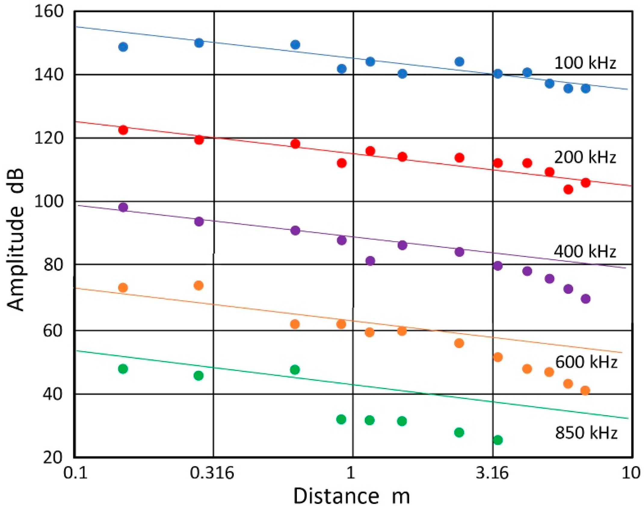
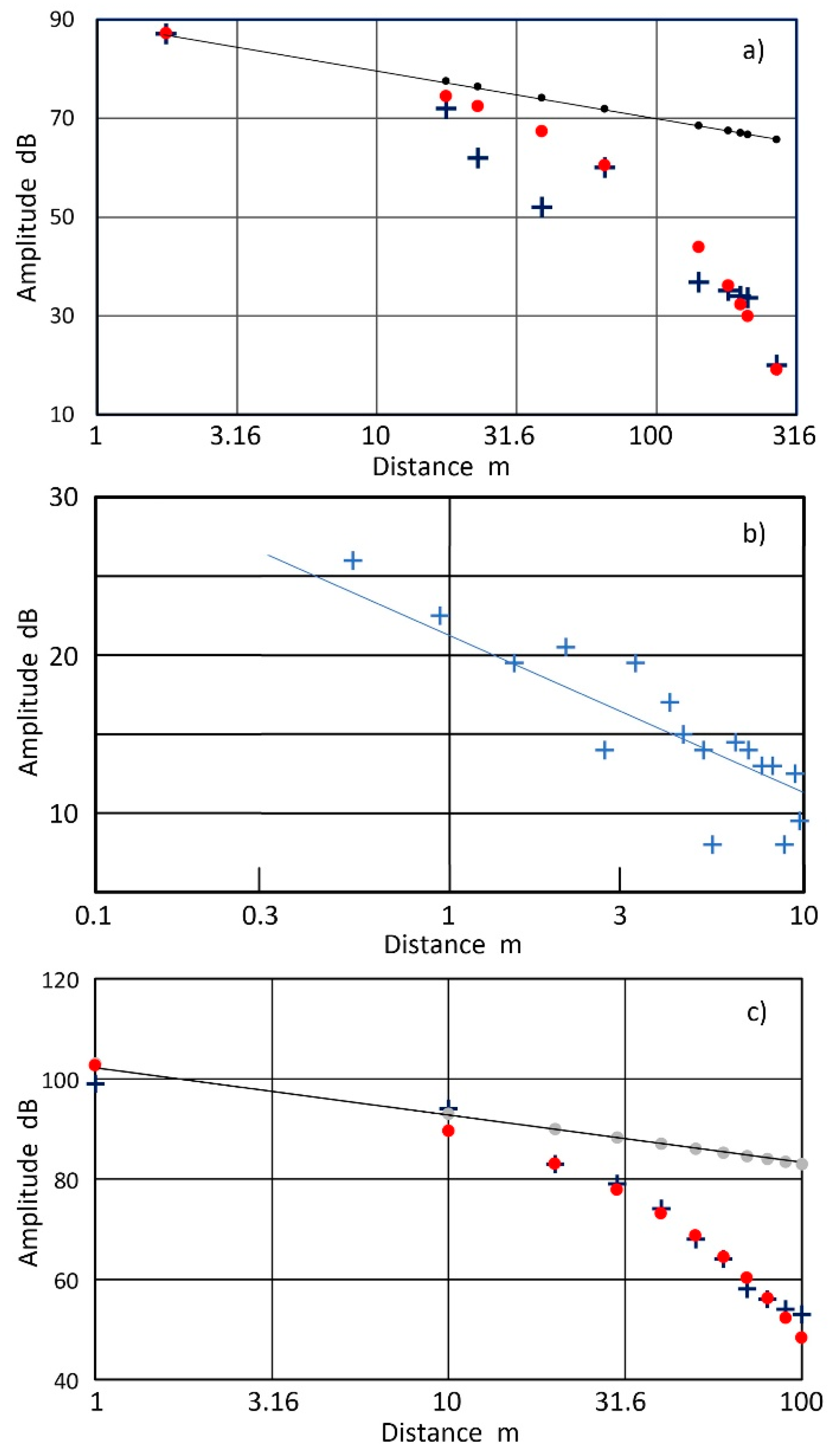
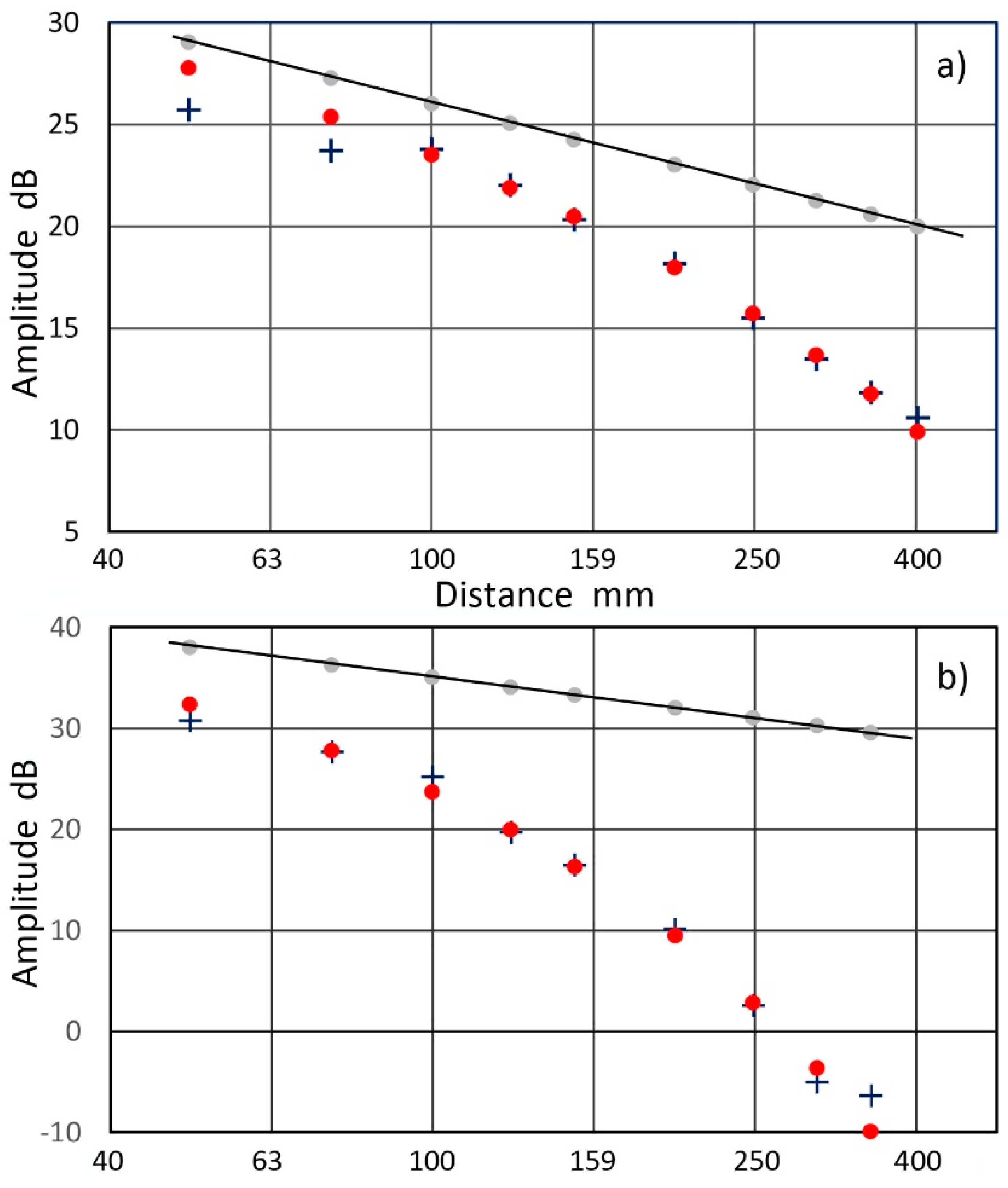
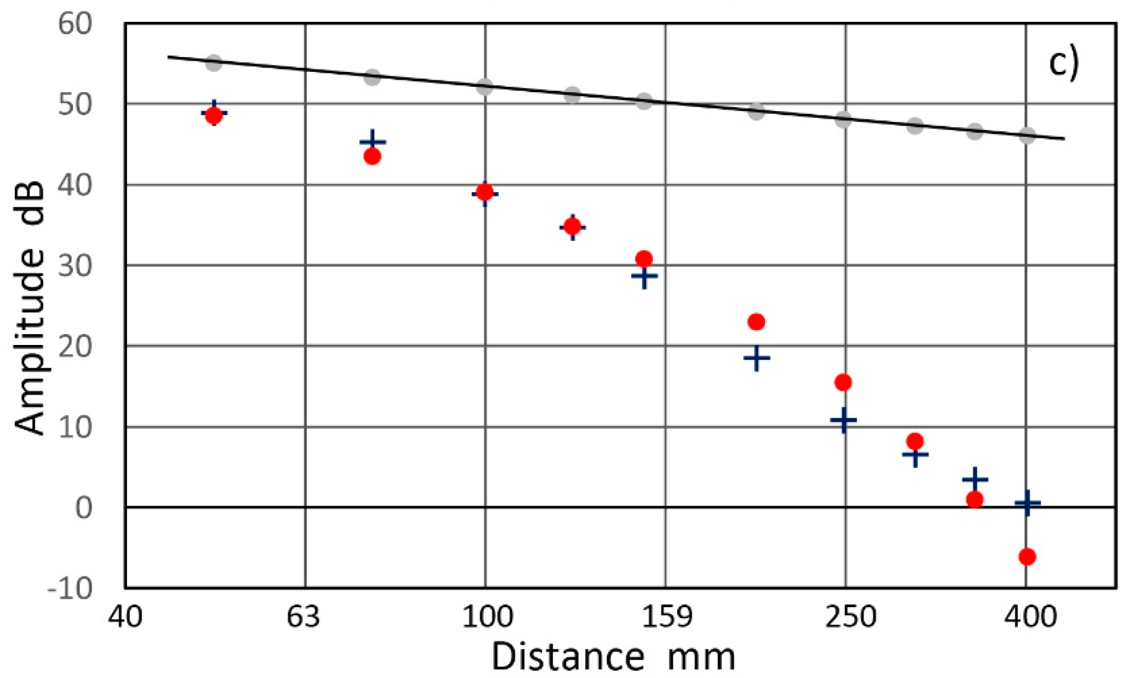
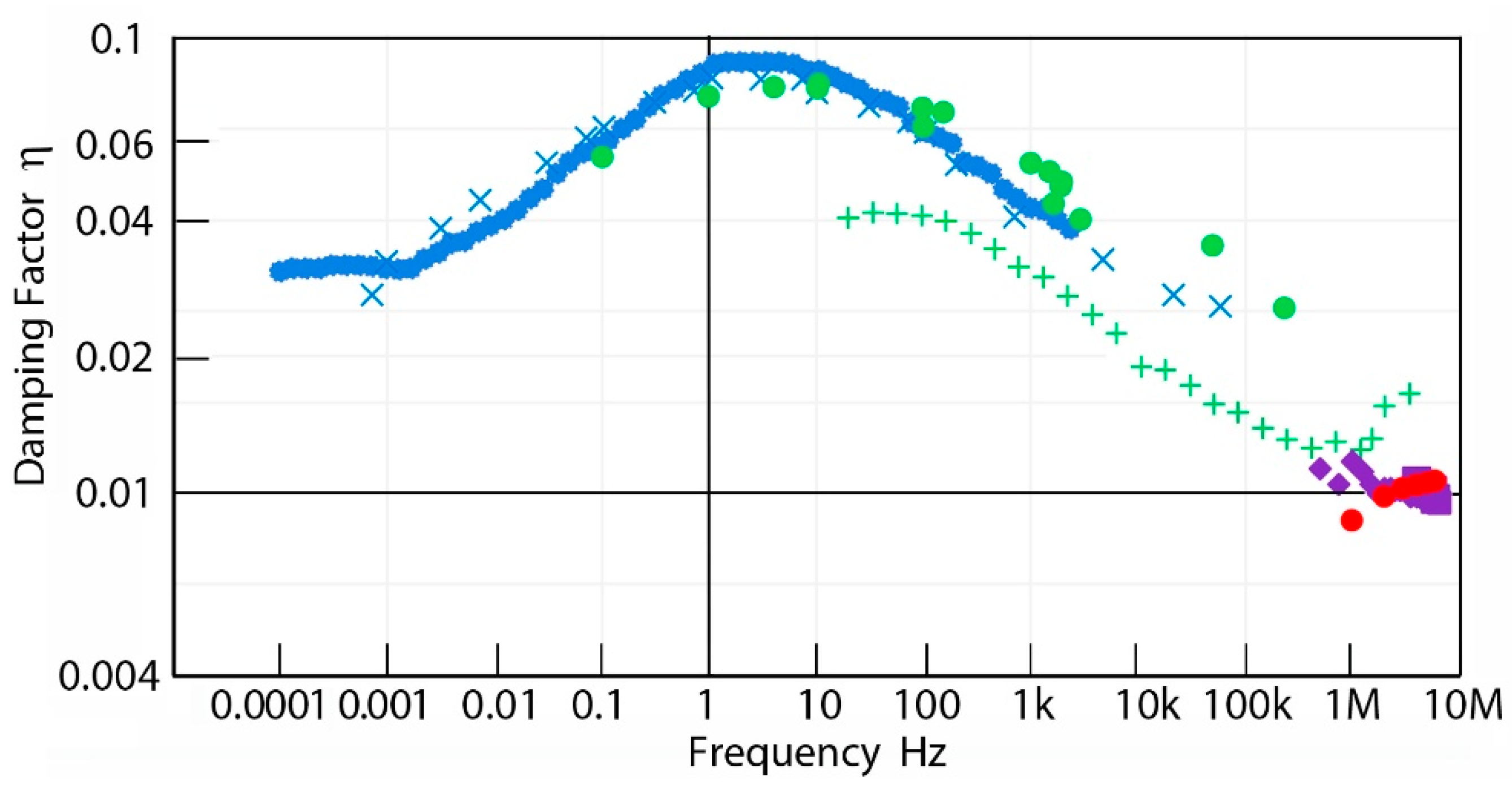
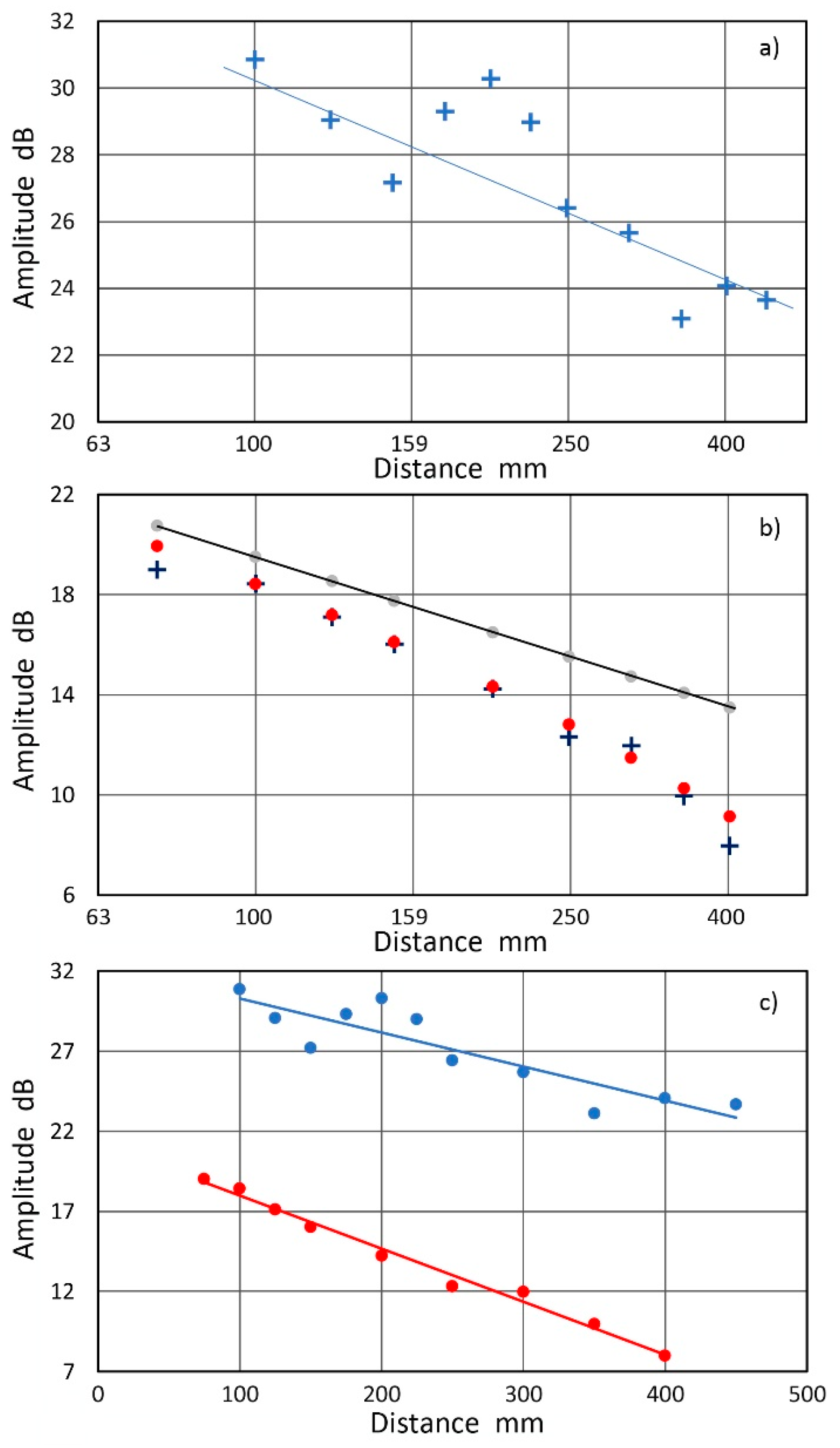
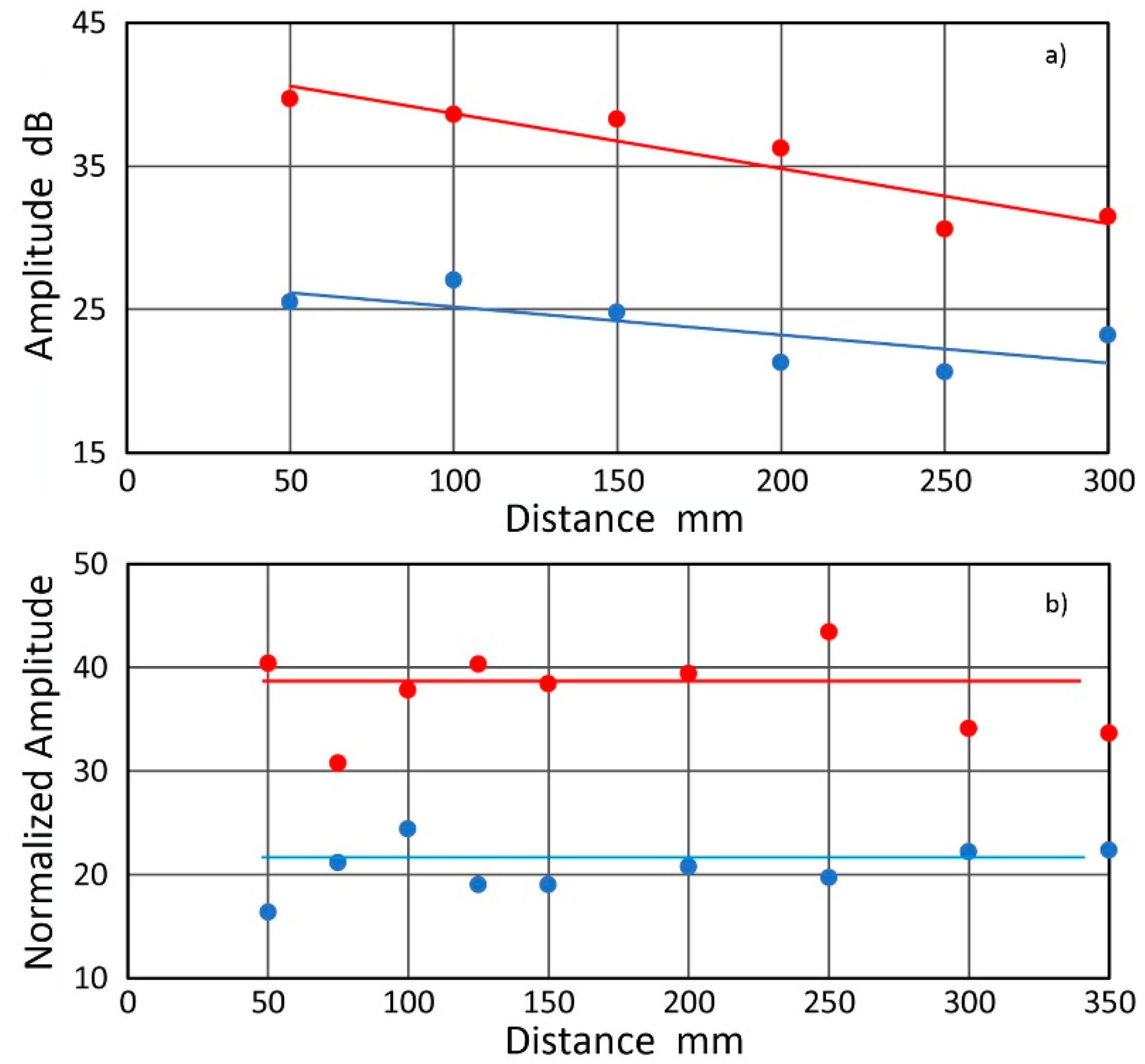
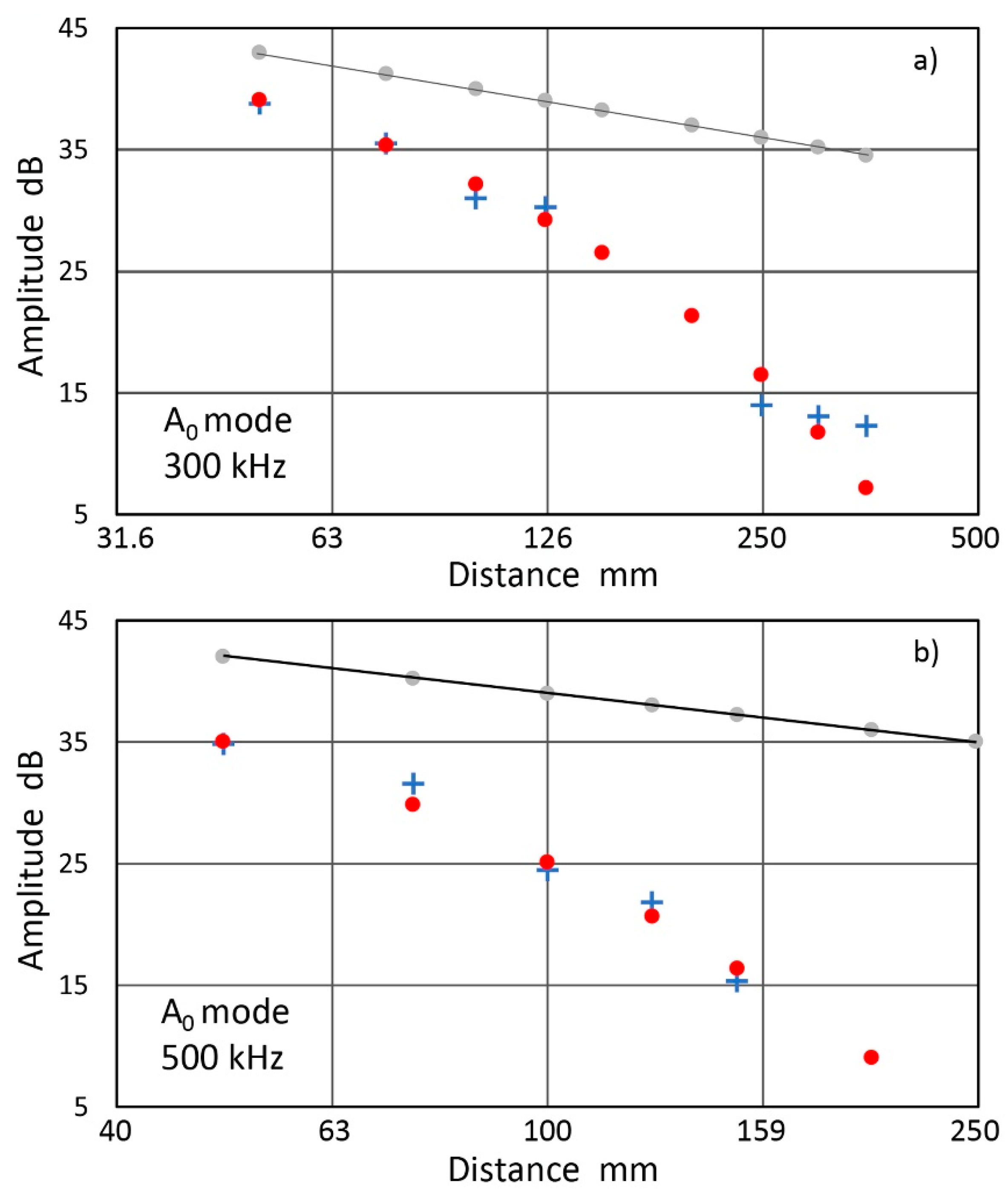
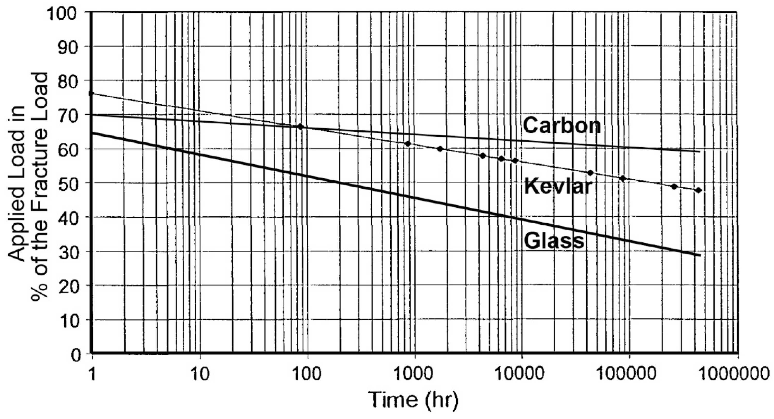
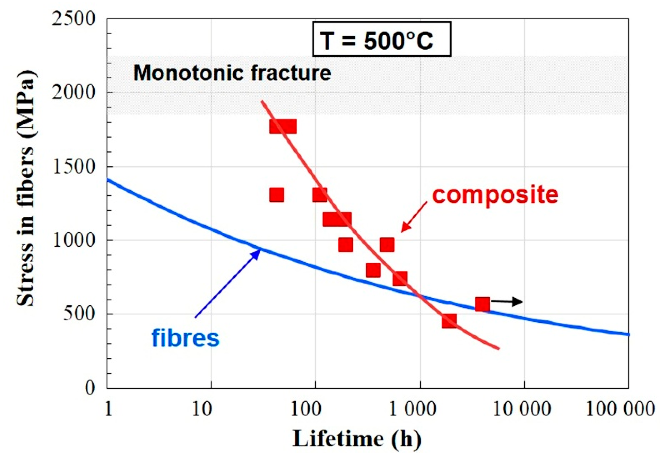
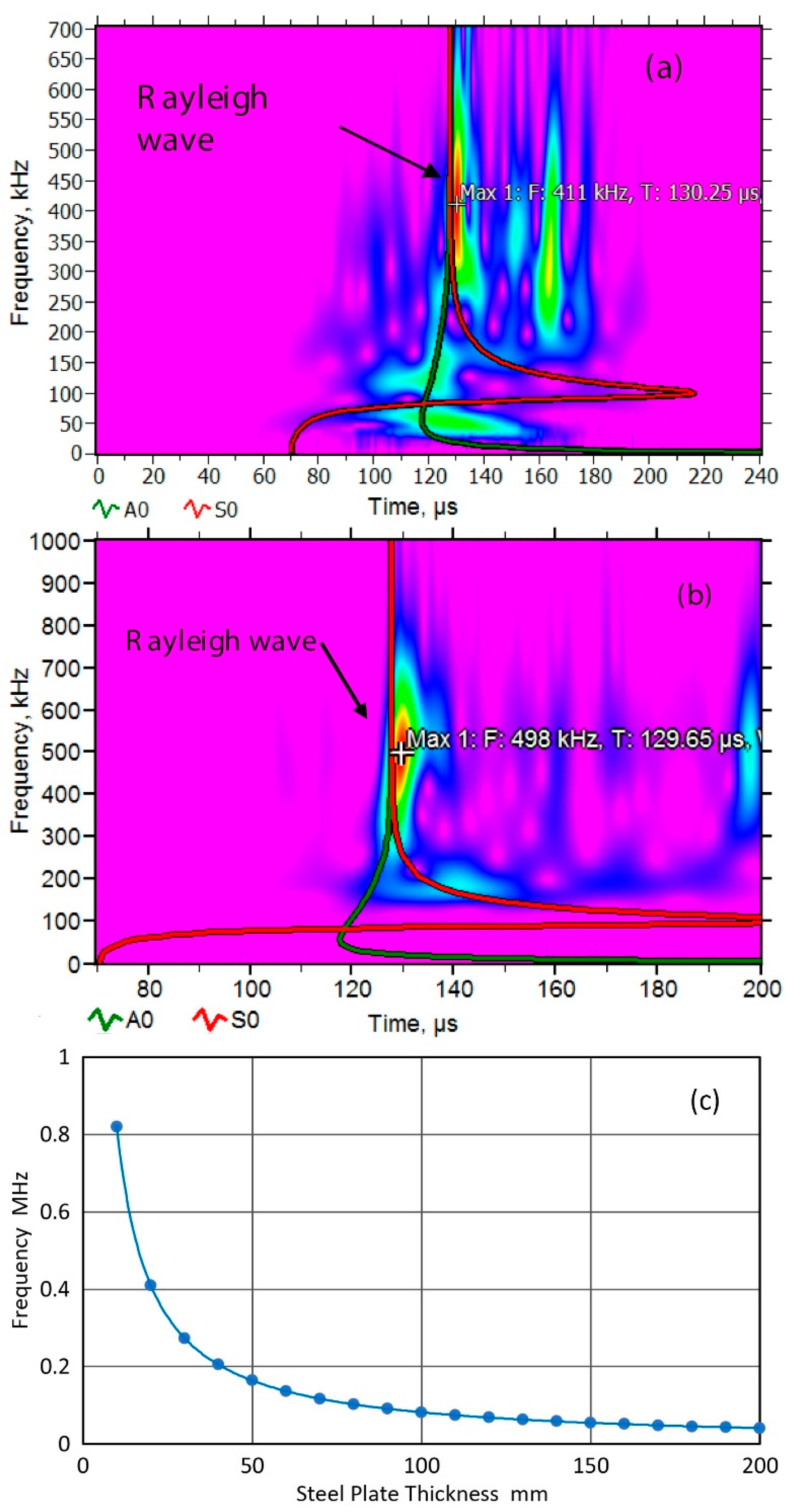
Table 1.
Damping factors from complex elastic moduli measurements
| Ref. No. 1 | Material | Axis 2 | η11 | η22 | η33 | η44 | η55 | η66 | H12 | η13 | η23 | Freq (MHz) |
|---|---|---|---|---|---|---|---|---|---|---|---|---|
| [60] | Epoxy | 0.01 | 0.01 | 0.011 | ||||||||
| [49] | PMMA | 0.023 | 0.056 | 0.026 | 0.046 | 0.3 | ||||||
| [49] | GFRP-UD | 3 | 0.047 | 0.043 | 0.033 | 0.050 | 0.038 | 0.033 | 0.036 | 0.3 | ||
| [61] | GFRP-UD | 3 | 0.051 | 0.038 | 0.056 | 0.100 | 0.070 | 0.091 | 0.014 | 0.106 | 0.05–0.2 | |
| [61] | CFRP-UD | 3 | 0.027 | 0.05 | 0.075 | 0.06 | 0.063 | 0.11 | 0.037 | 0.1 | 0.05–0.2 | |
| [62] | CFRP-UD | 1 | 0.061 | 0.024 | 0.046 | 0.084 | 0.062 | 0.055 | 0.114 | 0.105 | 0.029 | |
| [63] | CFRP-UD | 1 | 0.086 | 0.045 | 0.06 | 0.037 | 0.033 | 0.005–0.2 | ||||
| [64] | CFRP-UD | 1 | 0.024 | 0.043 | 0.041 | 0.032 | 0.056 | 0.093 | 0.143 | 0.074 | 0.2–0.93 | |
| [64] | CFRP-QI | 1 | 0.041 | 0.067 | 0.034 | 0.045 | 0.044 | 0.068 | 0.071 | 0.016 | 0.2–0.93 | |
| [65,66] | CFRP XP | 1 | 0.020 | 0.018 | 0.001 | 0.010 | 0.017 | 0.026 | 0.018 | 0.016 | 0.001 | 0.01–1 |
| [65,66] | CFRP-UD | 1 | 0.015 | 0.099 | 0.099 | 0.010 | 0.045 | 0.045 | 0.015 | 0.015 | 0.261 | 0.01–1 |
1: Ref. No. refers to reference number. 2: Axis indicates the coordinate direction along fiber direction (0° orientation in QI-quasi-isotropic or XP-cross-ply).
Table 2.
Ultrasonic attenuation of engineering alloys
| Material | Type | α-p 1 | α-t 1 | Method 2 | Condition 3 | Reference | Ref. No. |
|---|---|---|---|---|---|---|---|
| Al | 1100 (2S) | 0.16 (5), 1(10) | Q | Hikata (1957) | [82] | ||
| Al | Al (99.99%) | 28 (6.3) | E | Anneal 200 °C 1 h | Hirao (2003) | [76] | |
| 2017 (17ST) | 5.6 (5) | 13.1 (4) | Q | GS: 0.23 mm | Mason (1947) | [26] | |
| 2017 (17ST) | 2.6 (5) | 7.9 (5) | Q | GS: 0.13 mm | Mason (1947) | [26] | |
| Cu | Cu (99.99%) | 88 (2.3) | E | GS: 35 µm | Hirao (2003) | [76] | |
| Brass (360) | 45.7 (10) | 286 (5) | Q | GS: 49 µm | Papadakis (1965) | [43] | |
| Mg | -- | 32.3 (10) | Q | GS: 0.2 mm | Mason (1948) | [83] | |
| AZ31 (FS1) | 6.9 (10) | 4.1 (10) | Q | GS: 0.12 mm | Mason (1948) | [83] | |
| Nb | Nb | 280–510 (5) | GS: 43–124 µm | Zeng (2010) | [84] | ||
| Ni | Grade A | 115 (3.5) | 240 (2) | Q | GS: 55 µm | Papadakis (1965) | [43] |
| Waspaloy | 51 (4.5) | E | solution + aged | Ohtani (2004) | [75] | ||
| Fe | Fe-0.004%C | 339 (8.2) | GS: 50 µm | Ahn (2000) | [85] | ||
| Fe-0.02%C | 300–1350 (10) | GS: 18–137 µm | Smith (1981) | [70] | |||
| Fe-0.06%C | 46–101 (5) | GS: 22–30 µm | Klinman (1980) | [68] | |||
| Steel | Fe-0.15%C | 33–60 (5) | GS: 14–40 µm | Klinman (1980) | [68] | ||
| Fe-0.15%C | 116 (5) | E | GS: 49 µm | Hirao (2003) | [76] | ||
| Fe-0.2%C | 220–340 (5) | GS: 120–290 µm | Ahn (2000) | [85] | |||
| Fe-0.25%C | 45–91 (5) | GS: 12–29 µm | Klinman (1980) | [68] | |||
| Fe-low C | 83–237 (5) | GS: 50–120 µm | Klinman (1980) | [68] | |||
| Fe-0.4%C | 53 (5) | GS: 12–20 µm | Klinman (1980) | [68] | |||
| Fe-0.4%C | 86–127 (5) | GS: 50–65 µm | Klinman (1980) | [68] | |||
| 4150 | 78.7 (10) | RHC: 14 | Roederick (1952) | [27] | |||
| 4150 | 19.7 (20) | RHC: 61 | Roederick (1952) | [27] | |||
| 4145 | 14.5 (5) | Q | VHN: 746 | Kamigaki (1957) | [28] | ||
| 4145 | 22.5 (5) | Q | VHN: 265 | Kamigaki (1957) | [28] | ||
| 3140 | 21.2 (10) | Q | RHC: 45 | Papadakis (1960) | [30] | ||
| 4150 | 21.2 (10) | Q | RHC: 54 | Papadakis (1960) | [30] | ||
| 4150 | 12.2 (10) | Q | pearlie-bainite | Papadakis (1964) | [29] | ||
| 4150 | 6.4 (20) | Q | martensite (M) | Papadakis (1964) | [29] | ||
| 4150 | 11.0 (20) | Q | tempered M | Papadakis (1964) | [29] | ||
| 1Cr-Mo-V | 33 (5) | E | tempered M | Ohtani (2002) | [77] | ||
| 2.25Cr-1Mo | 25.6 (3.9) | E | annealed | Ohtani (2006) | [78] | ||
| 1075 | 10 (5) | Q | GSc: 27 µm | Kamigaki (1957) | [28] | ||
| 1075 | 35 (5) | Q | GSc: 38 µm | Kamigaki (1957) | [28] | ||
| 1075 | 68 (5) | Q | GSc: 68 µm | Kamigaki (1957) | [28] | ||
| 1075 | 174 (5) | Q | GSc: 174 µm | Kamigaki (1957) | [28] | ||
| 1075 | 73.5 (10) | Q | VHN: 696 | Kamigaki (1957) | [28] | ||
| 1075 | 90 (10) | Q | VHN: 274 | Kamigaki (1957) | [28] | ||
| 1075 | 174 (10) | Q | VHN: 270 | Kamigaki (1957) | [28] | ||
| 1080 | 19.2–33.9 (10) | Q | spheroidized | Latiff (1974) | [83] | ||
| 1080 | 230–290 (5) | normalized | Ahn (2000) | [85] | |||
| Rail steel | 26–150 (10) | Quenched | Du (2014) | [86] | |||
| 52100 | 2.4–22 (10) | 6.8–44 (10) | Q | RHC: 55–61 | Papadakis (1970) | [72] | |
| Plain C | 150–1000 (15) | GS: 15–33 µm | Smith (1983) | [71] | |||
| Plain C | 150–1690 (10) | GS: 10–31 µm | Klinman (1981) | [69] | |||
| 316L SS | 230 (5), 360 (10) | GS: 37 µm | Wan (2017) | [87] | |||
| 316L SS | 5.0 (5) | E | GS: 19.5 µm | Ohtani (2005) | [79] | ||
| 403 SS | 26 (10) | Q | GSc: 25 µm | Nadeau (1985) | [88] | ||
| 416 SS | 27.8 (5) | 159 (5) | Q | GS: 30 µm | Papadakis (1965) | [43] | |
| 416 SS | 348 (10) | Q | GS: 30 µm | Papadakis (1965) | [43] | ||
| 440C austenitic SS | 313 (5) | 814 (5) | Q | GS: 50 µm | Papadakis (1965) | [43] | |
| Cast austenitic SS | 192 (0.5), 174 (1) | columnar 2.5 mm | Ramuhalli (2009) | [89] | |||
| Cast austenitic SS | 264 (0.5), 272 (1) | equiaxed 2.3 mm | Ramuhalli (2009) | [89] |
1 Attenuation coefficient is given in dB/m, followed by frequency in MHz in the parentheses. In many cases, results for additional frequencies are given as well. 2 Q refers to measurement method using quartz discs and E using electromagnetic transducer. 3 GS: grain size, GSc: pearlite colony size or prior austenite grain size, VHN: Vickers hardness number, RHC: Rockwell hardness-C-scale, M: martensite.
© 2018 by the author. Licensee MDPI, Basel, Switzerland. This article is an open access article distributed under the terms and conditions of the Creative Commons Attribution (CC BY) license (http://creativecommons.org/licenses/by/4.0/).
Share and Cite
MDPI and ACS Style
Ono, K. Review on Structural Health Evaluation with Acoustic Emission. Appl. Sci. 2018, 8, 958. https://doi.org/10.3390/app8060958
AMA Style
Ono K. Review on Structural Health Evaluation with Acoustic Emission. Applied Sciences. 2018; 8(6):958. https://doi.org/10.3390/app8060958
Chicago/Turabian StyleOno, Kanji. 2018. "Review on Structural Health Evaluation with Acoustic Emission" Applied Sciences 8, no. 6: 958. https://doi.org/10.3390/app8060958
Note that from the first issue of 2016, this journal uses article numbers instead of page numbers. See further details here.