A Multi-Frame PCA-Based Stereo Audio Coding Method

Abstract

With the increasing demand for high quality audio, stereo audio coding has become more and more important. In this paper, a multi-frame coding method based on Principal Component Analysis (PCA) is proposed for the compression of audio signals, including both mono and stereo signals. The PCA-based method makes the input audio spectral coefficients into eigenvectors of covariance matrices and reduces coding bitrate by grouping such eigenvectors into fewer number of vectors. The multi-frame joint technique makes the PCA-based method more efficient and feasible. This paper also proposes a quantization method that utilizes Pyramid Vector Quantization (PVQ) to quantize the PCA matrices proposed in this paper with few bits. Parametric coding algorithms are also employed with PCA to ensure the high efficiency of the proposed audio codec. Subjective listening tests with Multiple Stimuli with Hidden Reference and Anchor (MUSHRA) have shown that the proposed PCA-based coding method is efficient at processing stereo audio.

1. Introduction

The goal of audio coding is to represent audio in digital form with as few bits as possible while maintaining the intelligibility and quality required for particular applications [1]. In audio coding, it is very important to deal with the stereo signal efficiently, which can offer better experiences of using applications like mobile communication and live audio broadcasting. Over these years, a variety of techniques for stereo signal processing have been proposed [2,3], including M/S stereo, intensity stereo, joint stereo, and parametric stereo.

M/S stereo coding transforms the left and right channels into a mid-channel and a side channel. Intensity stereo works on the principle of sound localization [4]: humans have a less keen sense of perceiving the direction of certain audio frequencies. By exploiting this characteristic, intensity stereo coding can reduce the bitrate with little or no perceived change in apparent quality. Therefore, at very low bitrate, this type of coding usually yields a gain in perceived audio quality. Intensity stereo is supported by many audio compression formats such as Advanced Audio Coding (AAC) [5,6], which is used for the transfer of relatively low bit rate, acceptable-quality audio with modest internet access speed. Encoders with joint stereo such as Moving Picture Experts Group (MPEG) Audio Layer III (MP3) and Ogg Vorbis [7] use different algorithms to determine when to switch and how much space should be allocated to each channel (the quality can suffer if the switching is too frequent or if the side channel does not get enough bits). Based on the principle of human hearing [8,9], Parametric Stereo (PS) performs sparse coding in the spatial domain. The idea behind parametric stereo coding is to maximize the compression of a stereo signal by transmitting parameters describing the spatial image. For stereo input signals, the compression process basically follows one idea: synthesizing one signal from the two input channels and extracting parameters to be encoded and transmitted in order to add spatial cues for synthesized stereo at the receiver’s end. The parameter estimation is made in the frequency domain [10,11]. AAC with Spectral Band Replication (SBR) and parametric stereo is defined as High-Efficiency Advanced Audio Coding version 2 (HE-AACv2). On the basis of several stereo algorithms mentioned above, other improved algorithms have been proposed [12], which causes Max Coherent Rotation (MCR) to enhance the correlation between the left channel and the right channel, and uses MCR angle to substitute the spatial parameters. This kind of method with MCR reduces the bitrate of spatial parameters and increases the performance of some spatial audio coding, but has not been widely used.

Audio codec usually uses subspace-based methods such as Discrete Cosine Transform (DCT) [13], Fast Fourier Transform (FFT) [14], and Wavelet Transform [15] to transfer audio signal from time domain to frequency domain in suitably windowed time frames. Modified Discrete Cosine Transform (MDCT) is a lapped transform based on the type-IV Discrete Cosine Transform (DCT-IV), with the additional property of being lapped. Compared to other Fourier-related transforms, it has half as many outputs as inputs, and it has been widely used in audio coding. These transforms are general transformations; therefore, the energy aggregation can be further enhanced through an additional transformation like PCA [16,17], which is one of the optimal orthogonal transformations based on statistical properties. The orthogonal transformation can be understood as a coordinate one. That is, fewer new bases can be selected to construct a low dimensional space to describe the data in the original high dimensional space by PCA, which means the compressibility is higher. Some work was done on the audio coding method combined with PCA from different views. Paper [18] proposed a novel method to match different subbands of the left channel and the right channel based on PCA, through which the redundancy of two channels can be reduced further. Paper [19] mainly focused on the multichannel procession and the application of PCA in the subband, and it discussed several details of PCA, such as the energy of each eigenvector and the signal waveform after PCA. This paper introduced the rotation angle with Karhunen-Loève Transform (KLT) instead of the rotation matrix and the reduced-dimensional matrix compared to our paper. The paper [20] mainly focused on the localization of multichannel based on PCA, with which the original audio is separated into primary and ambient components. Then, these different components are used to analyze spatial perception, respectively, in order to improve the robustness of multichannel audio coding.

In this paper, a multi-frame, PCA-based coding method for audio compression is proposed, which makes use of the properties of the orthogonal transformation and explores the feasibility of increasing the compression rate further after time-frequency transition. Compared to the previous work, this paper proposes a different method of applying PCA in audio coding. The main contributions of this paper include a new matrix construction method, a matrix quantization method based on PVQ, a combination method of PCA and parametric stereo, and a multi frame technique combined with PCA. In this method, the encoders transfer the matrices generated by PCA instead of the coefficients of the frequency spectrum. The proposed PCA-based coding method can hold both a mono signal and a stereo signal combined with parametric stereo. With the application of the multi-frame technique, the bitrate can be further reduced with a small impact on quality. To reduce the bitrate of the matrices, a method of matrix quantization based on PVQ [21] is put forward in this paper.

The rest of the paper is organized as follows: Section 2 describes the multi-frame, PCA-based coding method for mono signals. Section 3 presents the proposed design of the matrix quantization. In Section 4, the PCA-based coding method for the mono signal is extended to stereo signals combined with improved parametric stereo. The experimental results, discussion, and conclusion are presented in Section 5, Section 6 and Section 7, respectively.

2. Multi-Frame PCA-Based Coding Method

2.1. Framework of PCA-Based Coding Method

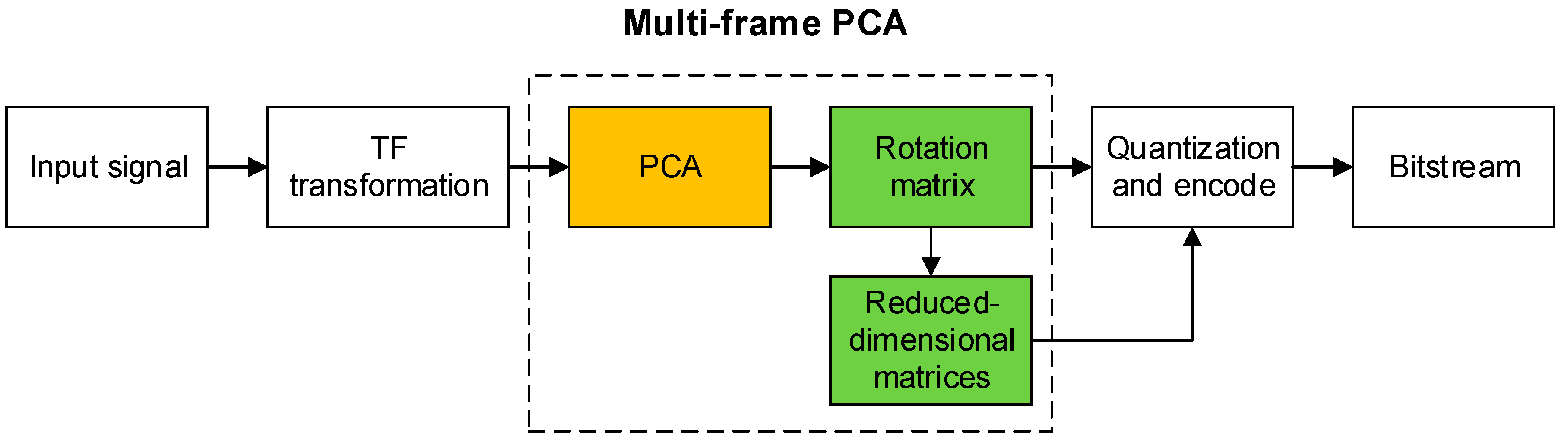
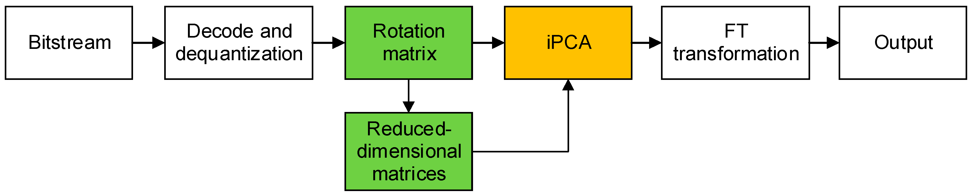
The encoding process can be described as follows: after time-frequency transformation such as MDCT, the frequency coefficients are used in the module of PCA, which includes the multi-frame technique. Several matrices are generated after PCA is quantized and encoded to bitstream. The decoder is the mirror image of the encoder, after decoding and de-quantizing, matrices are used to generate frequency domain signals by inverse PCA (iPCA). Finally, after frequency-time transformation, the encoder can export audio. Flowcharts of encoder and decoder for mono signals are shown in Figure 1 and Figure 2. The part of MDCT is used to concentrate energy of signal on low band in frequency domain, which is good for the process of matrix construction (details are shown in Section 2.4). Some informal listening experiments have been carried out on the performance applying PCA without MDCT. The experimental results show that without MDCT, the performance of PCA has slight reduction, which means more bits are needed by the scheme without MDCT in order to achieve the same output quality of the scheme with MDCT. Thus, in this paper MDCT is assumed to enhance the performance of the PCA, although it will bring more computational complexity.

2.2. Principle of PCA

The PCA’s mathematical principle is as follows: after coordinate transformation, the original high-dimensional samples with certain relevance can be transferred to a new set of low-dimensional samples that are unrelated to each other. These new samples carry most information of the original data and can replace the original samples for follow-up analysis.

There are several criteria for choosing new samples or selecting new bases in PCA. The typical method is to use the variance of new sample F₁ (i.e., the variance of the original sample mapping on the new coordinates). The larger Var (Fi) is, the more information Fi contains. So, the first principal component should have the largest variance F₁. If the first principal component F₁ is not qualified to replace the original sample, then the second principal component F₂ should be considered. F₂ is the principal component with the largest variance except F₁, and F₂ is uncorrelated to $F_1$, that is, $\mathrm{Cov}\left(F_1,F_2\right)=0$. This means that the base of F₁ and the base of F₂ are orthogonal to each other, which can reduce the data redundancy between new samples (or principal components) effectively. The third, fourth, and p-th principal component can be constructed similarly. The variance of these principal components is in descending order, and the corresponding base in new space is uncorrelated to other new base. If there are m n-dimensional data, the procession of PCA is shown in

Table 1. PCA ALGORITHM.

Algorithm: PCA (Principle Component Analysis)
(i) Obtain matrix by columns: $X_{\left[\begin{array}{cc}m& n\end{array}\right]}$
(ii) Zero-mean columns in $X_{\left[\begin{array}{cc}m& n\end{array}\right]}$ to get matrix X
(iii) Calculate C = $\frac{1}{m}{X}^{T}X$
(iv) Calculate eigenvalues ${\lambda }_1,{\lambda }_2,{\lambda }_3\dots {\lambda }_n$ and eigenvectors $a_1,a_2,a_3\dots a_n$ of C
(v) Use eigenvector to construct $P_{\left[\begin{array}{cc}n& n\end{array}\right]}$ according to the eigenvalue
(vi) Select the first k columns of $P_{\left[\begin{array}{cc}n& n\end{array}\right]}$ to construct the rotation matrix $P_{\left[\begin{array}{cc}n& k\end{array}\right]}$
(vii) Complete dimensionality reduction by $Y_{\left[\begin{array}{cc}m& k\end{array}\right]}=X_{\left[\begin{array}{cc}m& n\end{array}\right]}\times P_{\left[\begin{array}{cc}n& k\end{array}\right]}$

.

The contribution rate of the principal component reflects the proportion that each principal component accounts for the total amount of data after coordinate transformation, which can effectively solve the problem of dimension selection after dimensionality reduction. In PCA application, people often use the cumulative contribution rate as the basis for principal components selection. The cumulative contribution rate $M_k$ of the first k principal components is

$$M_k=\frac{{{\displaystyle \sum }}_{i=1}^k{\lambda }_i}{{{\displaystyle \sum }}_{i=1}^n{\lambda }_i}$$

(1)

If the contribution rate of the first k principal components meets the specific requirements (the contribution rates are different according to different requirements), the first k principal components can be used to describe the original data to achieve the purpose of dimensionality reduction.

PCA is a good transformation due to its properties, as follows:

(i)

Each new base is orthogonal to the other new base;

(ii)

Mean squared error of the data is the minimum after transformation;

(iii)

Energy is more concentrated and more convenient for data processing.

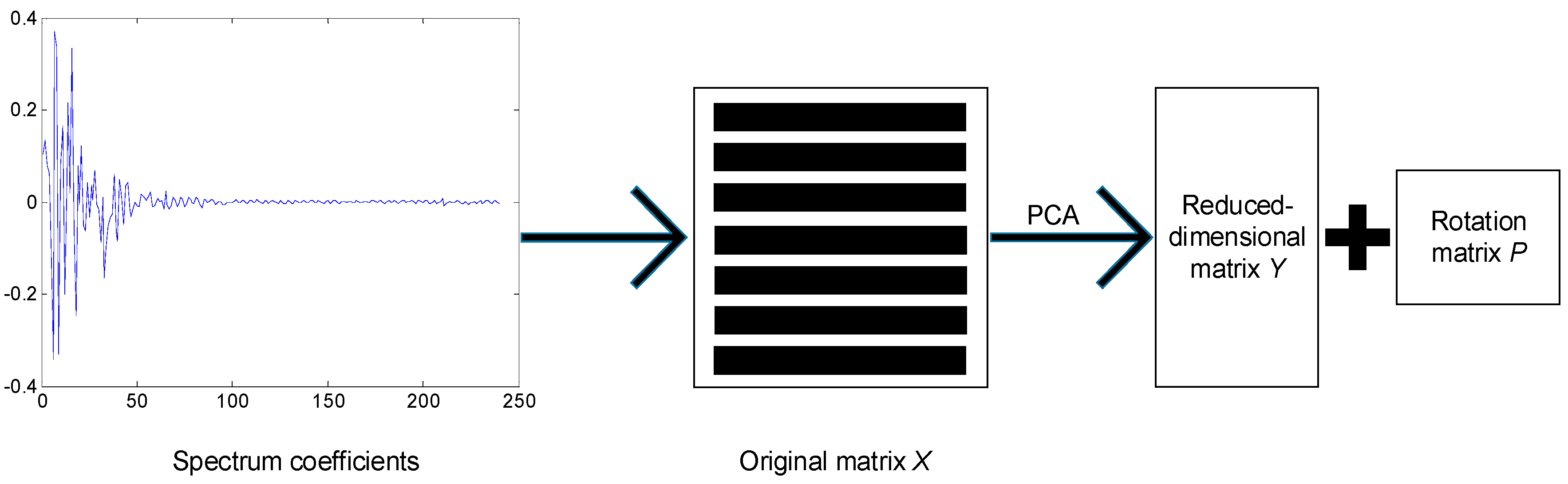
It is worthwhile noting that PCA does not simply delete the data of little importance. After PCA transformation, the dimension-reduced data can be transformed to restore most of the high-dimensional original data, which is a good character for data compression. In this paper, as is shown in Figure 3, the spectrum coefficients of the input signal are divided into multiple samples according to specific rules; then, these samples will be constructed to the original matrix X. After the principal component analysis, matrix X is decomposed into reduced-dimensional matrix Y and rotation matrix P; the process of calculating matrix Y and P is shown in Table 1. The matrix Y and P are transmitted to the decoder after quantization and coding. In decoder, the original matrix can be restored by multiplying reduced-dimensional matrix and transposed rotation matrix. There is some data loss during dimension reduction, but the loss is much less, so we can ignore it. For example, we can recover 99.97% information through a 6-dimension matrix, when the autocorrelation matrix has the 15th dimension. Ideally the original matrix X can be restored by reduced-dimensional matrix Y and rotation matrix P with

$$X\approx X_{restore}=Y\times P^T$$

(2)

in which $X_{restore}$ is the matrix restored in decoder and $P^T$ is the transposition rank of matrix P. Then, $X_{restore}$ is reconstructed to spectral coefficients.

2.3. Format of Each Matrix

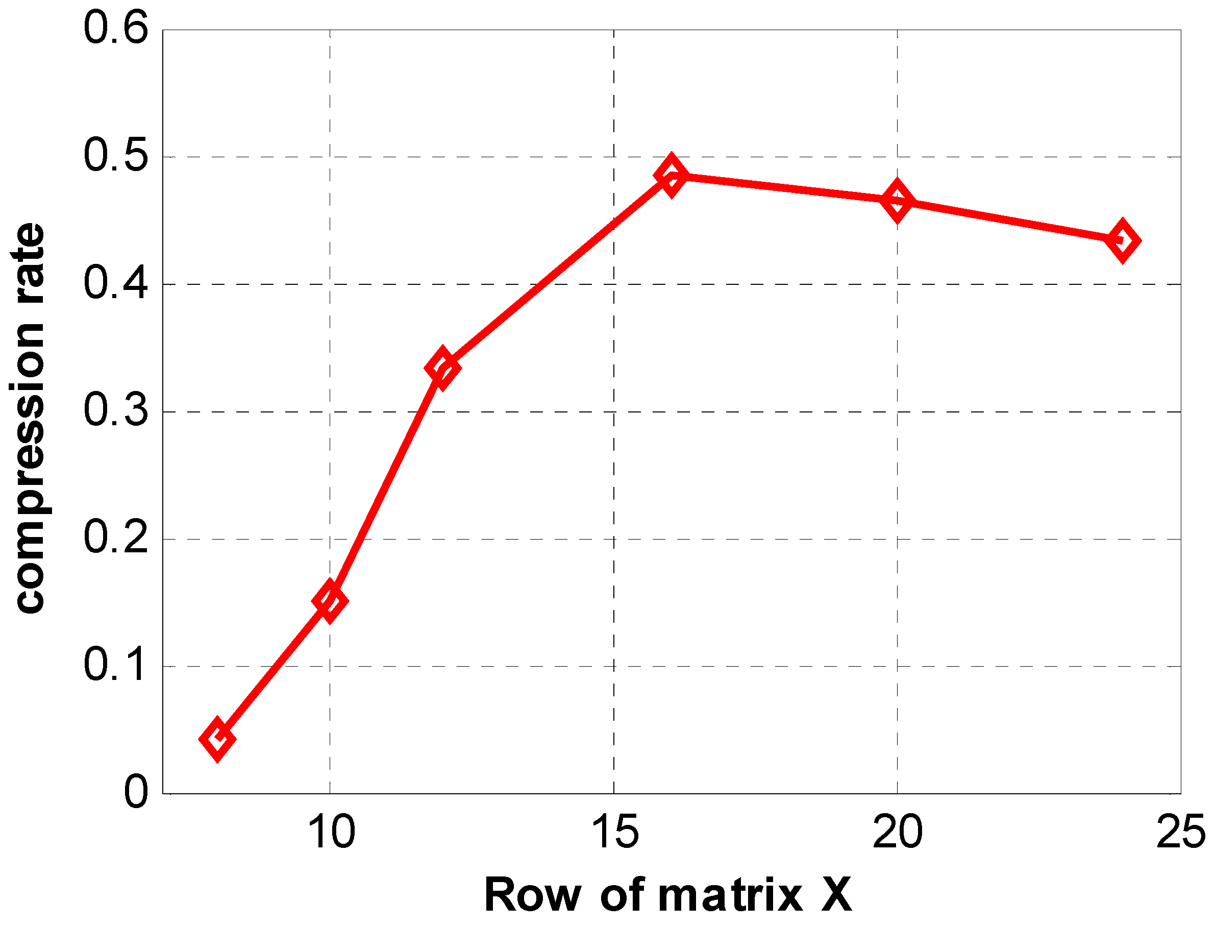
In encoder, when the sampling rate is 48 kHz, the frame has 240 spectral coefficients after MDCT (in this paper, the MDCT frame size is 5 ms with 50% overlap). There are many forms of matrices like 6 × 40, 12 × 20, 20 × 12, and so on; each format of matrix brings different compression rates. In a simple test, several formats of original matrix were constructed. Then, a subjective test was devised using those different dimensional rotation matrices. 10 listeners recorded the number of dimensions when the restored audio had acceptable quality. Then, the compression rate was calculated by the number of dimensions. As is shown in Figure 4, the matrix has the largest compression rate when it has 16 rows. So, the matrix $X_{\left[\begin{array}{cc}16& 15\end{array}\right]}$ with 16 rows and 15 columns is selected for transient frame in this paper. That means a 240-coefficient-long frequency domain signal is divided into 16 samples, each sample having 15 dimensions.

2.4. Way of Matrix Construction

An appropriate way to obtain the 16 samples from frequency domain coefficients is necessary. This paper proposes one method as follows: suppose the coefficients of one frame in frequency domain are $a_{1,}{a}_2\dots a_{240}$. $a_1$ is filled in the first column and the first row $X_{\left[\begin{array}{cc}1& 1\end{array}\right]}$, $a_2$ is filled in the first column and the second row $X_{\left[\begin{array}{cc}2& 1\end{array}\right]}$, and $a_{16}$ is filled in the first column and the 16th row $X_{\left[\begin{array}{cc}16& 1\end{array}\right]}$. Then, $a_{17}$ is filled in the first row and second column $X_{\left[\begin{array}{cc}1& 2\end{array}\right]}$, $a_{18}$ is filled in the second row and second column $X_{\left[\begin{array}{cc}2& 2\end{array}\right]}$, and so on, until all the coefficients have been filled in the original matrix $X_{\left[\begin{array}{cc}16& 15\end{array}\right]}$; that is,

$$X_{\left[\begin{array}{cc}16& 15\end{array}\right]}=\left[\begin{array}{ccc}{a}_{1,}& \cdots & a_{225}\\ ⋮& \ddots & ⋮\\ a_{16,}& \cdots & a_{240}\end{array}\right]$$

(3)

This method has two obvious advantages, which can be find in Figure 5:

(i) This method takes advantage of the short-time stationary characteristic of signals in the frequency domain. Therefore, the difference between different rows in the same column of the matrix constructed by this sampling method is small. In other words, the difference between the same dimensions of different samples in the matrix is small, and different dimensions have similar linear relationships, which is very conducive to dimensionality reduction.

(ii) This method allows signal energy to gather still in the low-dimensional region of the new space. The energy of the frequency domain signal is concentrated in the low frequency region; after PCA, the advanced column of reduced-dimensional matrix still has the most signal energy. Thus, after dimensionality reduction, we can still focus on the low-dimensional region.

2.5. Multi-Frame Joint PCA

In the experiment, a phenomenon was observed that the rotation matrices of adjacent frames are greatly similar. Therefore, it is possible to do joint PCA with multiple frames to generate one rotation matrix, that is, multiple frames use the same rotation matrix. Therefore, the codec can transmit fewer rotation matrices, and bitrate can be reduced.

Below is one way to do joint PCA with least error. First, frequency domain coefficients of n sub-frames are constructed as n original matrices ${X_1}_{\left[\begin{array}{cc}16& 15\end{array}\right]}$, ${X_2}_{\left[\begin{array}{cc}16& 15\end{array}\right]}\dots {X_n}_{\left[\begin{array}{cc}16& 15\end{array}\right]},$ respectively; then, the original matrices of each sub-frame are used to form one original matrix $X_{\left[\begin{array}{cc}16n& 15\end{array}\right]}$. This matrix is used to obtain one rotation matrix and n reduced-dimensional matrices.

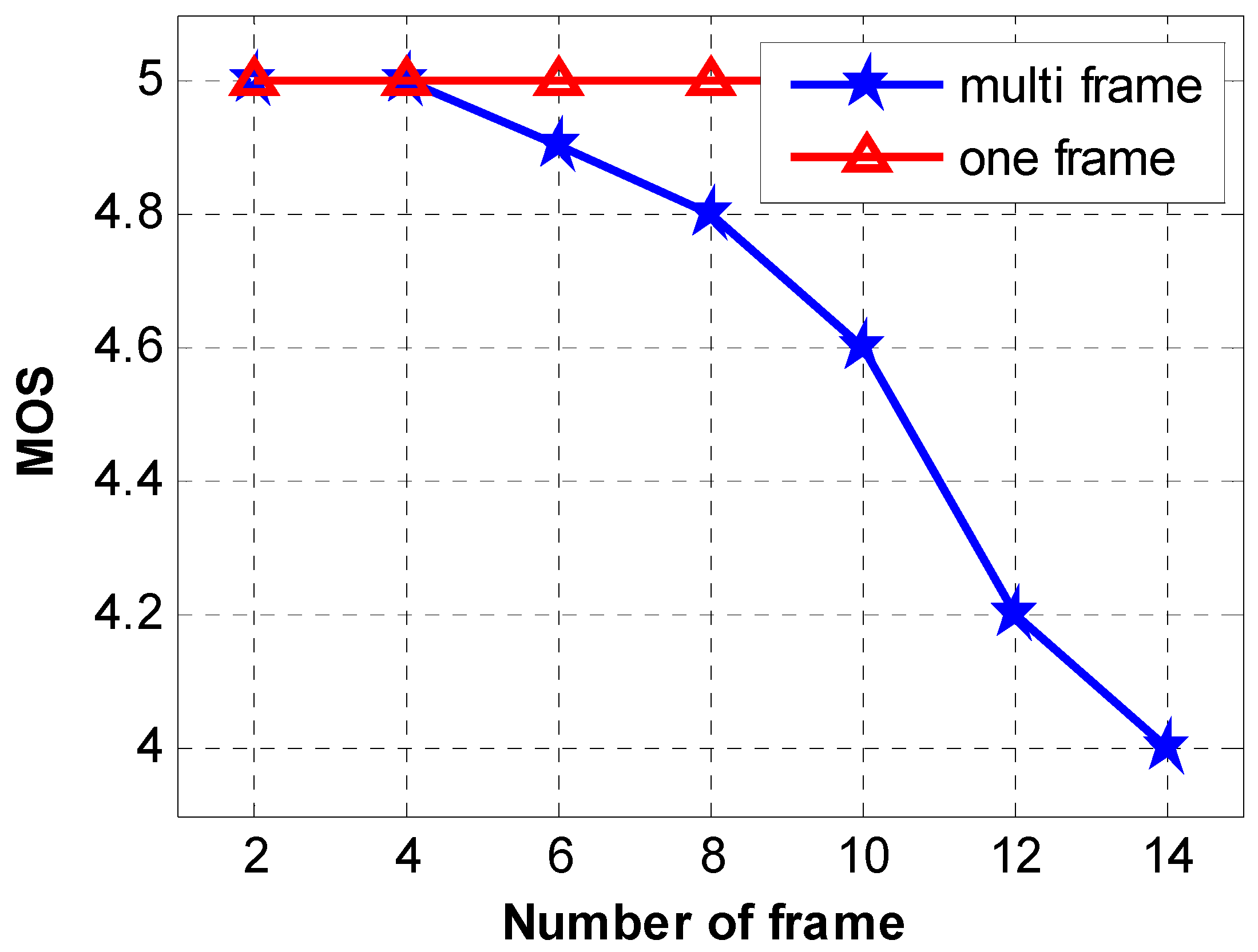
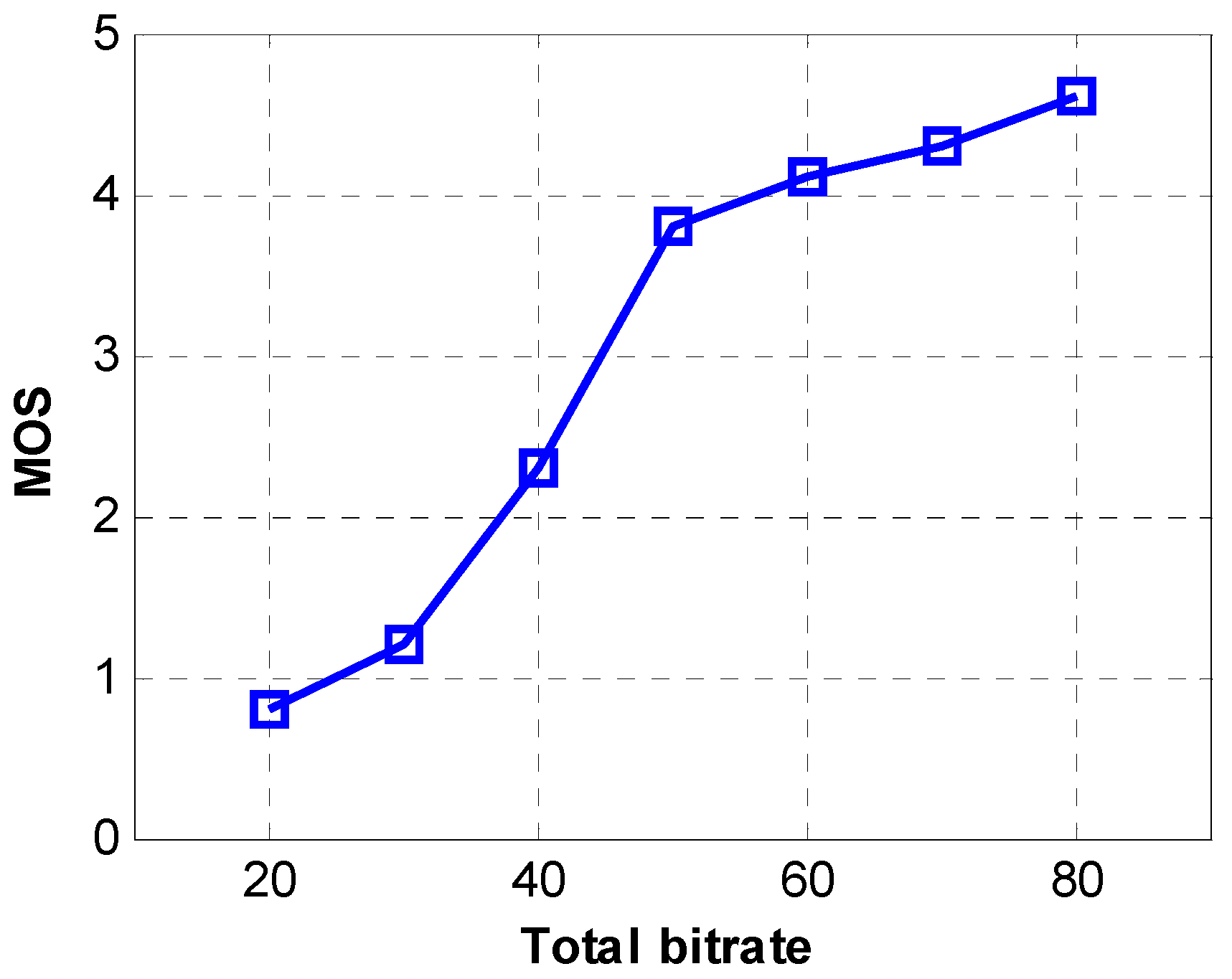
If too many matrices are analyzed at the same time, the codec delay will be high, which is unbearable for real-time communication. Besides, the average quality of restored audio signal decreases with the increase in the number of frames. Therefore, the need to reduce bitrate and real-time communication should be comprehensively considered. A subjective listening test was designed to find the relationship between the number of frames and the quality of restored signal. 10 audio materials from European Broadcasting Union (EBU) test materials were coded with multi-frame PCA with different numbers of frames. The Mean Opinion Score (MOS) [22] of the restored music was recorded by 10 listeners. The statistical results are shown in Figure 6.

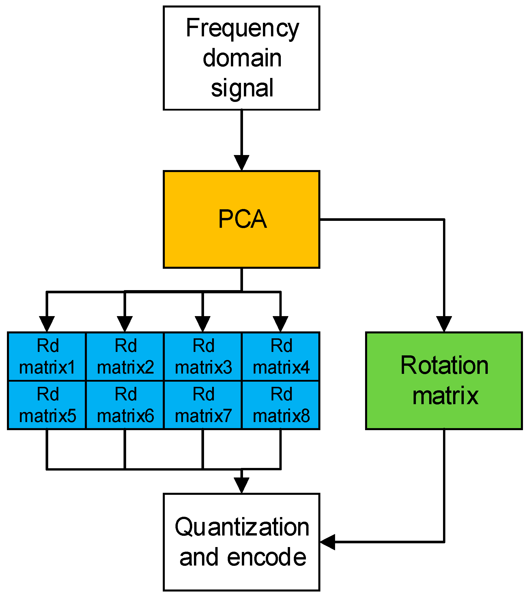
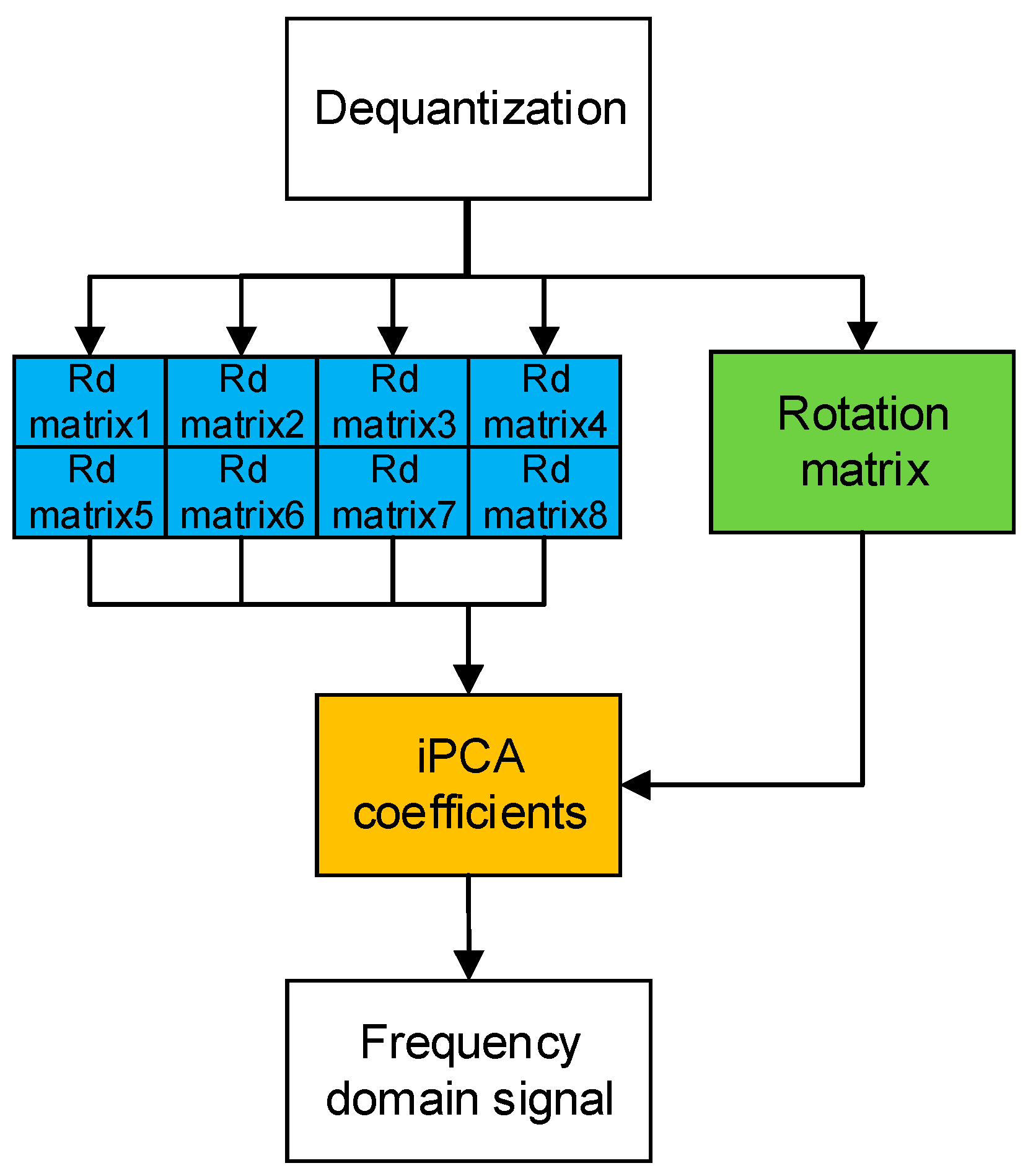
As is shown in Figure 6, when the number of frames is less than 6 or 8, the decrease of audio quality is not obvious. A suitable number of frames is then subjected to joint PCA. Taken together, when 8 sub-frames are analyzed at the same time, the bitrate and the delay of encoder is acceptable, that is, for every 40 ms signal, 8 sub-frame reduced-dimensional (Rd) matrices and one rotation matrix are transferred. Main functions of the mono encoder and decoder combined with multi-frame joint PCA are shown in Figure 7 and Figure 8. In encoder, 40 ms signal is used to produce 8 Rd matrices and 1 rotation matrix. In decoder, after receiving 8 Rd matrices and 1 rotation matrix, 8 frames are restored to generate 40 ms signal.

3. Quantization Design Based On PVQ

According to the properties of matrix multiplication, if the error of one point in matrix Y or P is large, the restored signal may have a large error. Therefore, uniform quantization cannot limit the error of every point in the matrix in the acceptable range with bitrate limitation. So, it is necessary to set a series of new quantization rules based on the properties of the dimensionality matrix and the rotation matrix. It is assumed that the audio signal obeys the distribution of Laplace [23], and both PCA and MDCT in the paper are orthogonal transformations. Thus, the distribution of matrix coefficients is maintained in Laplace distribution. Meanwhile, we have observed the values in reduced-dimensional matrix and rotation matrix. It is shown that most values of cells in matrix are close to 0, and the bigger the absolute value, the smaller the probability is. Based on the above two statements, the distribution of coefficients in reduced-dimensional matrix and rotation matrix can be regarded as Laplace distribution. Lattice vector quantization (LVQ) is widely used in the codec because of its low computational complexity. PVQ is one method of LVQ that is suitable for Laplace distribution. Thus, this section presents a design of quantization for reduced-dimensional matrix and rotation matrix combined with PVQ.

3.1. Quantization Design of the Reduced-Dimensional Matrix

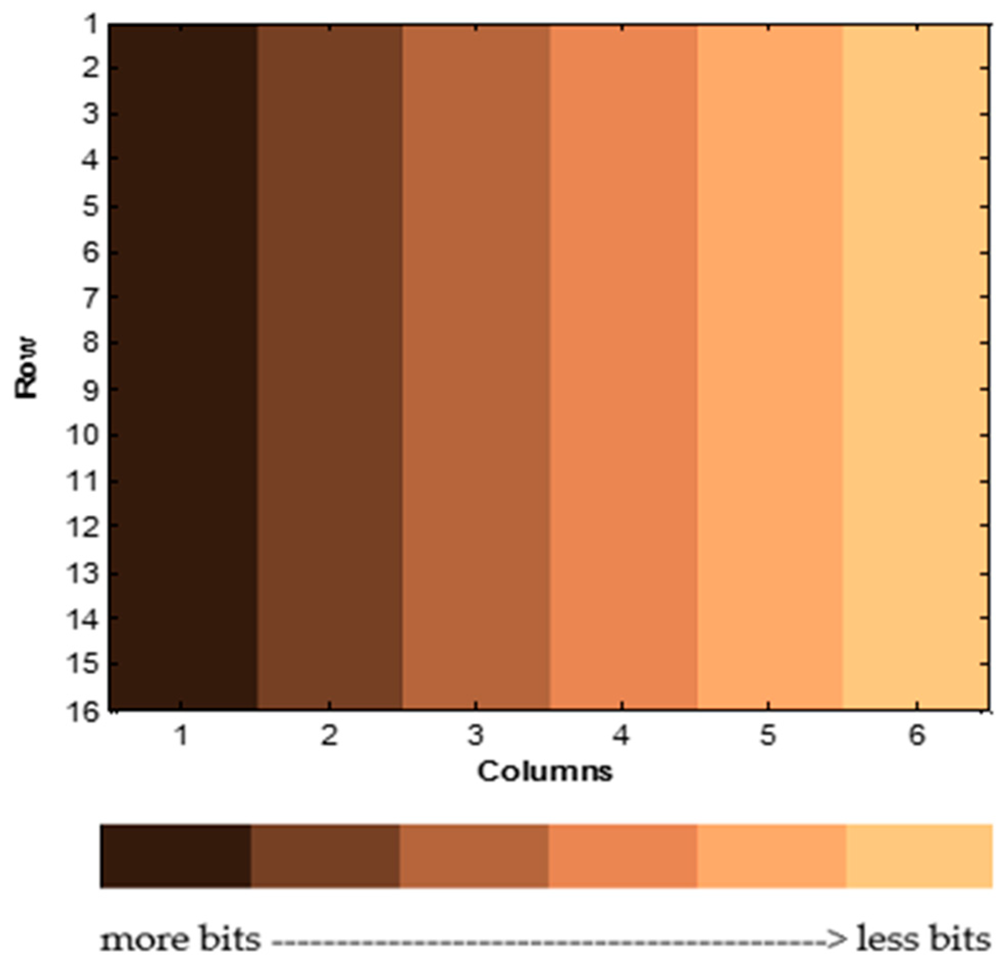
In the reduced-dimensional matrix, the first column is the first principal component, the second column is the second principal component, etc. According to the property of PCA, the first principal component has the most important information of the original signal, and information carried by other principal components becomes less and less important. In fact, more than 95% of the original signal energy, which can be also called information, is restored only by the first principal component. That means if the quantization error of the first principal component is large, compared with the original signal, the restored signal also has a large error. Therefore, the first principal component needs to be allocated more bits, and the bits for other principal components should be sequentially reduced. For some kinds of audio, 4 principal components are enough to obtain acceptable quality, while for other kinds of audio 5 principal components may be needed. We choose 6 principal components, because they can satisfy almost all kinds of audio. In fact, the fifth and sixth principal components play a small role in the restored spectral; therefore, little quantization accuracy is needed for the last two principal components.

Based on the above conclusion, the reduced dimensional matrix can be divided into certain regions, as is shown in Figure 9. Different regions have different bit allocations: the darker color means more bits needed.

A PVQ quantizer was used to quantify the distribution of different bits in each principal component of the reduced-dimensional matrix. Several subjective listening tests have been carried out, and the bits assignments policy is determined according to the quality of the restored audio under different bit assignments. Finally, the bits that need to be allocated for each principal component are determined.

Table 2. Quantization bit for reduced-dimensional matrix.

Principal Component	Bits Needed (bit/per Point)
First principal component	3
Second principal component	3
Third principal component	2.5
Fourth principal component	1.5
Fifth principal component	0.45
Sixth principal component	0.45

gives the number of bits required for each principal component of non-zero reduced-dimensional matrix under the PVQ quantizer.

3.2. Quantization Design of the Rotation Matrix

According to Y = XP in encoder and $X_{restore}=Y{P}^T$ in decoder, some properties of the rotation matrix can be found:

(i)

The higher row in matrix P is used to restore the region of higher frequencies in the restored signal.

(ii)

The first column in matrix P corresponds to the first principal component in the reduced-dimensional matrix. That means that the first column of the rotation matrix only multiplies with the first column (first principal component) of the reduced-dimensional matrix when calculating the restored signal in the decoder. The second column of the rotation matrix only multiplies with the second column (second principal component) of the reduced-dimensional matrix, and so on. According to the above properties of the rotation matrix, the quantization distribution of the rotation matrix has been made clearer, that is, the larger the row number is, and the larger the column number is, the fewer allocation bits there are.

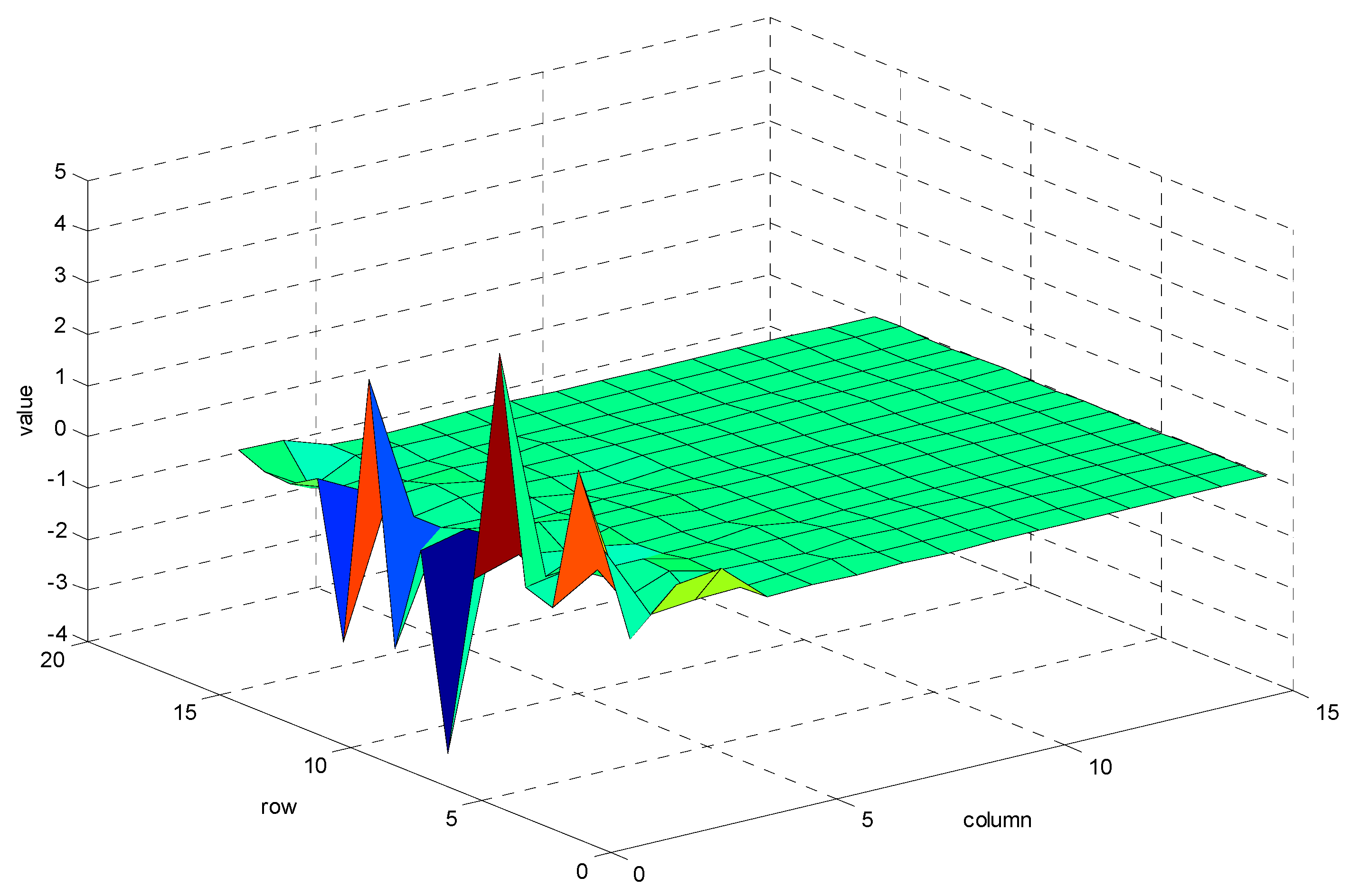
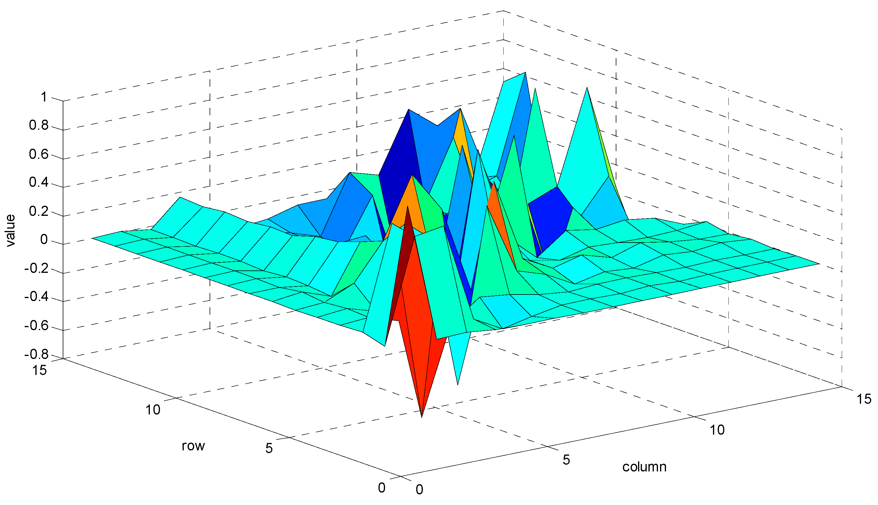
In addition to the above two properties of the rotation matrix, there is another important property. Generally, the data in the first four rows around the diagonal are bigger than others. The thinking of this characteristic in this paper is as follows: common audio focuses more energy on low-band in frequency domain, and the method of matrix construction described in Section 2.4 can keep the coefficients of low-band stay in low-column. Thus, the first diagonal value that is calculated from the first column must be the largest one of overall values in rotation matrix or autocorrelation matrix. The second diagonal value could quite possibly be the second-largest value, and so on. That means these data are more important for decoder, so the quantization accuracy of these regions with larger absolute values can determine the error between the restored signal and the original signal. Therefore, the data around the diagonal need to be allocated with more bits. Figure 10 shows the “average value” rotation matrix of a piece of audio as an example to show this property more clearly.

The rotation matrix also has the following quantization criterion:

(i)

The first column of the rotation matrix needs to be precisely quantized, because the first principal component of the reduced-dimensional signal is only multiplied by the first column of P in decoder to restore signal.

(ii)

Data in columns 2–6 in row 1 have little effect on the restored signal, so that few bits can be allocated for this region.

(iii)

The higher row in matrix P is used to restore the region of higher frequencies in the restored signal. The data in lines 13, 14, and 15 correspond to the frequency that exceeds the range of frequencies perceptible to the human ear, so these data do not need to be quantized.

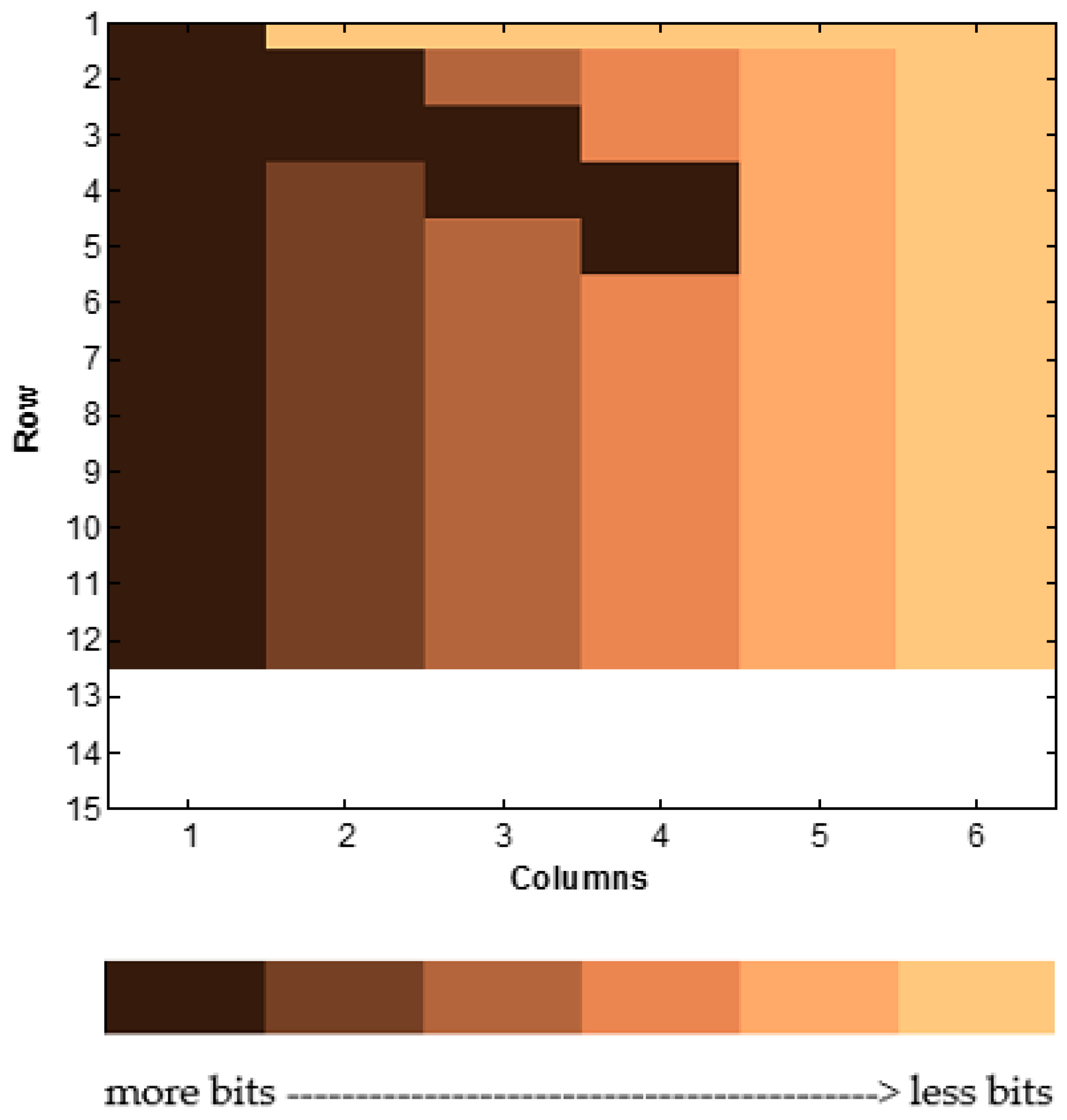
According to the above quantization criteria, the rotation matrix that is divided into the following regions according to bit allocation is shown in Figure 11. The darker the color is, the more bits should be allocated.

The same test method as the one for reduced-dimensional matrix was used to determine the number of bits needed in each region in rotation matrix.

In

Table 3. Quantization bits for rotation matrix.

Region	Bits Needed (bit/per Point)
The first region	4
The second region	3
The third region	2
The fourth region	2
The fifth region	0.5
The sixth region	0.5
The seventh region	0

, the first region corresponds to the region with the darkest color in Figure 11; the second corresponds to the area with the second-darkest color, and so on. The white color means there are no bits allocated to that area.

3.3. Design of the Low-Pass Filter

The noise generated from quantization and matrix calculation is white noise. There are two ways to reduce it. The first way is introducing noise shaping to make noise more comfortable for human hearing, and the second way is introducing a filter in decoder.

For most signals, the energy concentrates on low frequency domain, therefore the noise in low frequency domain does not sound obvious because of simultaneous masking. While in the high frequency part, if the original signal does not have high frequency components, the noise signal will not be masked and can be heard. So, a low-pass filter can be set to mask the high frequency noise signal, without affecting the original signal. The key point of the filter design is to determine the cut-off frequency.

Given the original matrix $X_{\left[\begin{array}{cc}16& 15\end{array}\right]}=\left[\begin{array}{ccc}{a}_1& \dots & a_{225}\\ ⋮& \ddots & ⋮\\ a_{16}& \dots & a_{240}\end{array}\right]$, there are 15 subbands in X, in which the first subband is the first row, the second subband is the second row, and so on. When $\mathrm{C}=\frac{1}{m}{X}^{T}X$ is calculated in PCA, the first value $e_1$ on the diagonal line $e_1,e_2\dots e_{15}$ is calculated by

$$\begin{array}{cc}\hfill e_1& =((a_1-\overline{a})\ast (a_1-\overline{a})+(a_2-\overline{a})\ast (a_2-\overline{a})+\dots (a_{16}-\overline{a})\ast (a_{16}-\overline{a}))/16\hfill \\ \hfill & =({a_1}^2+{a_2}^2+\dots {a_{16}}^2+16{\overline{a}}^2-2\overline{a}(a_1+a_2+\dots a_{16}))/16\hfill \\ \hfill & =({a_1}^2+{a_2}^2+\dots {a_{16}}^2-16{\overline{a}}^2)/16\hfill \end{array}$$

(4)

in which ${a_1}^2+{a_2}^2+\dots {a_{16}}^2$ is equal to the energy of the first subband $E_1$, and $\overline{a}$ is the average value of the first subband. Therefore, the relationship between $E_1$ and $e_1$ is

$$E_1=16(e_1+{\overline{a}}^2)$$

(5)

Actually, the value of ${\overline{a}}^2$ is far less than $e_1$, so $E_1$ is equal to 16$e_1$, and the relationships between $E_2\dots E_{15}$ and $e_2\dots e_{15}$ can be gotten by analogy. Therefore, through PCA, the energy of each subband is calculated, and the filter can be determined by the energy of each band. Considering the proportion of energy accumulation, $A_k$ is

$$A_k=\frac{{{\displaystyle \sum }}_{i=1}^k{e}_i}{{{\displaystyle \sum }}_{i=1}^{15}{e}_i}$$

(6)

According to some experiments, when $A_k=99.6\%$, k is the proper cut-off band. When the signal passes through the filter, the noise signal will be filtered out, and the signal itself will not be too much damaged.

Considering the frequency characteristics of the audio signal, the stop band setting is not low, and the signal with more than 20,000 Hz is often ignored by default, so each band of the above 15 bands will not be transmitted. Taken together, $e_1,e_2,e_3,e_{12},e_{13},e_{14},e_{15}$ will not be transmitted, and the index of the left 8 bands are quantized by 3 bits, so the bitrate for cut-off band is 75 bps.

4. PCA-Based Parametric Stereo

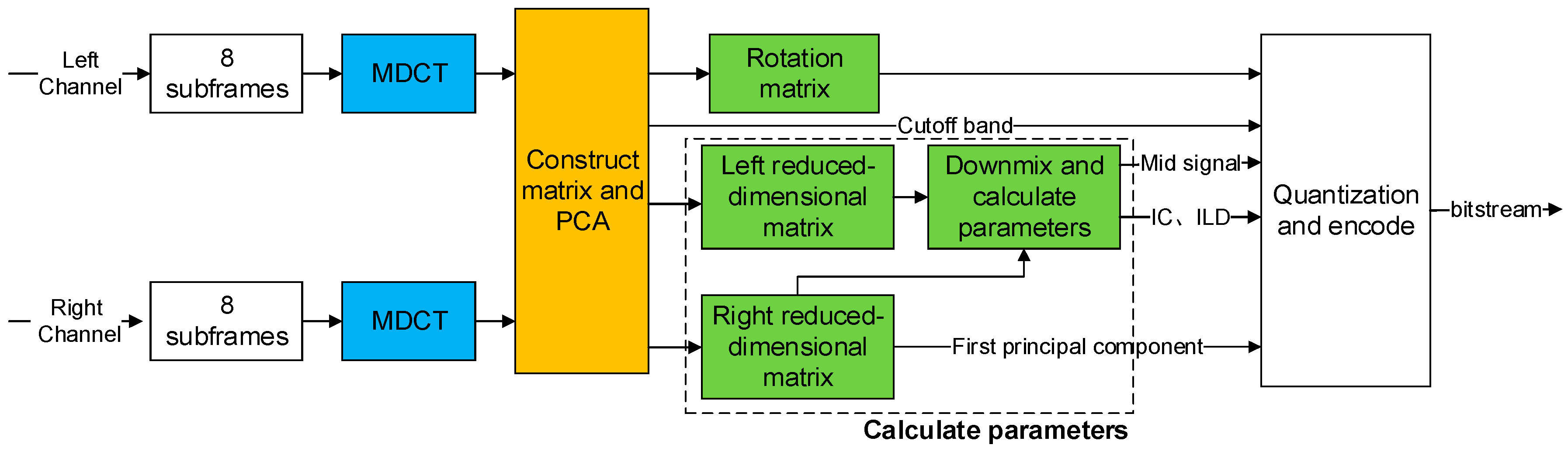
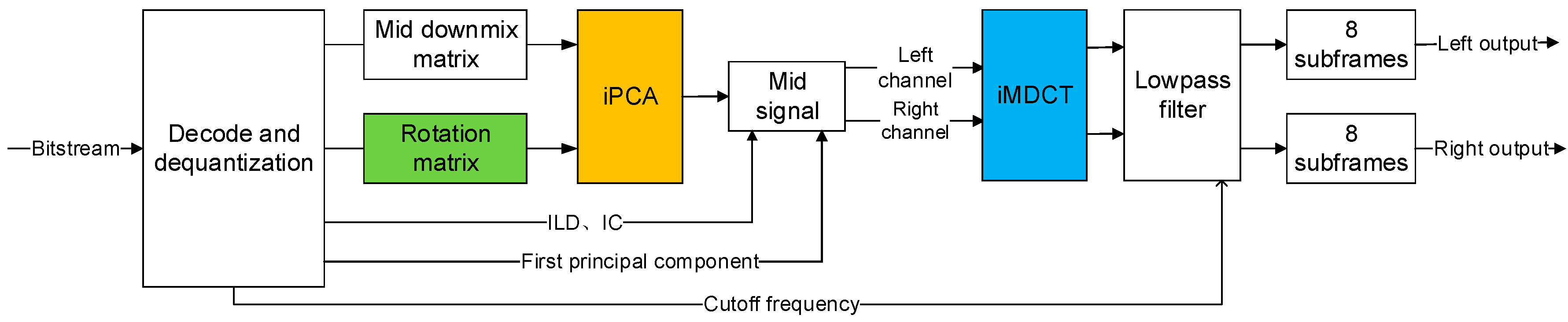
The stereo coding method proposed in this paper, as the extension of mono coding method mentioned before, is shown in Figure 12 and Figure 13. The encoder and decoder for stereo audio use the same module of PCA and quantization as mono audio. The differences between mono coding and stereo coding are elaborated in the following sections. In encoder, the two channels’ signal carries out MDCT and the two channels’ coefficients gather to generate an original matrix to do PCA; then, an improved parametric stereo module is used to downmix and calculate parameters of the high-band. Finally, a module based on PVQ is used for quantizing coefficients of matrix, and so on. In decoder, coefficients of mid downmix matrix and rotation matrix are used to generate mid channel; then, spatial parameters and other information are introduced to restore stereo signals. After inverse MDCT (iMDCT) and filtering, the signal can be regarded as the output signal.

4.1. Procession of Stereo Signal

Since the signals in two channels of the stereo tend to have high correlation. The signal of the left and right channels can be constructed into one original matrix. Firstly, the coefficients from left channel and right channel construct original matrices $X_{l\left[mn\right]}$ and $X_{l\left[mn\right]}$ respectively. Then, matrices $X_{l\left[mn\right]}$. and $X_{r\left[mn\right]}$ are used to form a new matrix X, in which $=\left[\begin{array}{c}{X}_{l\left[mn\right]}\\ X_{r\left[mn\right]}\end{array}\right]$. Matrix X is used to obtain one rotation matrix $P_{\left[nk\right]}$ by PCA, and $P_{\left[nk\right]}$ can handle both left and right channel signals. That is,

$$Y_{l\left[mk\right]}=X_{l\left[mn\right]}\times P_{\left[nk\right]}$$

(7)

$$Y_{r\left[mk\right]}=X_{r\left[mn\right]}\times P_{\left[nk\right]}$$

(8)

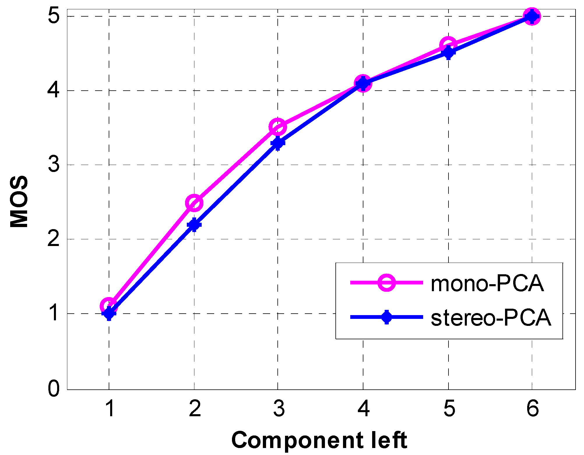
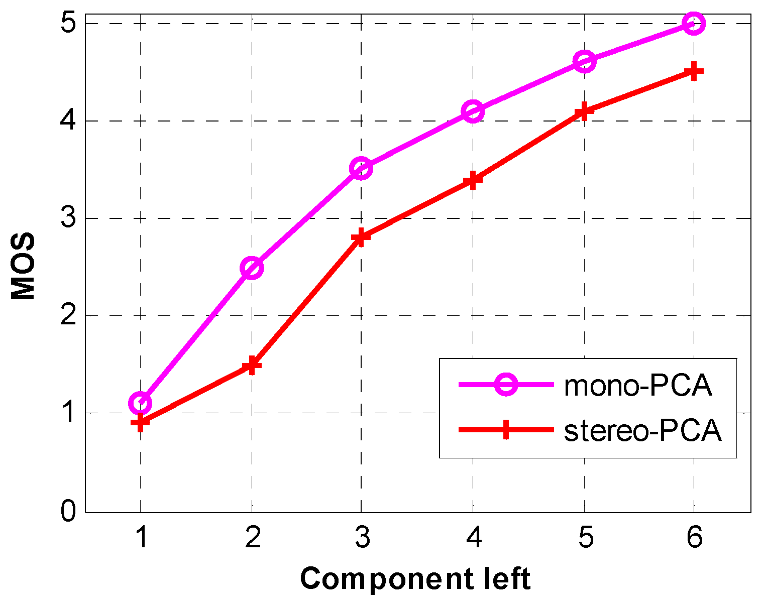
If the first six principal components are preserved, most mono audio signals can be well restored. At this time, we keep the first six bases in principal component matrix and obtain rotation matrix $P_{\left[\begin{array}{cc}15& 6\end{array}\right]}$. The reduced-dimensional matrices of each sub-frame are $Y_{1\left[156\right]},Y_{2\left[156\right]},\dots ,Y_{8\left[156\right]}$. Experiments were done to verify the design for stereo signals: 10 normal audio files and 5 artificial synthesized audio files (the left channel and right channel have less correlation) were chosen as the test materials. Results of the subjective listening experiments are shown in Figure 14 and Figure 15. We can consider that for most stereo signals, in which two channels have high relevance with each other, the proposed method for stereo signals perform as well as for mono signals.

4.2. Parameters in Parametric Stereo

In parametric stereo, Interaural Level Difference (ILD), Interaural Time Difference (ITD), and Interaural Coherence (IC) are used to describe the difference between two channels’ signals. In MDCT domain, the above parameters in subband b are calculated by:

$$\mathrm{ILD}\left[\mathrm{b}\right]=10lo{g}_{10}\frac{{{\displaystyle \sum }}_{k=A_{b-1}}^{A_b-1}{X}_l\left(k\right)X_l\left(k\right)}{{{\displaystyle \sum }}_{k=A_{b-1}}^{A_b-1}{X}_r\left(k\right)X_r\left(k\right)}$$

(9)

$$\mathrm{IC}\left[\mathrm{b}\right]=\mathrm{R}\left(X_{bl}\left(k\right),X_{br}\left(k\right)\right)=\frac{\langle X_{bl}\left(k\right),X_{br}\left(k\right)\rangle }{\left|X_{bl}\left(k\right)\right|\left|X_{br}\left(k\right)\right|}$$

(10)

While in MDCT domain, calculating ITD must introduce Modified Discrete Sine Transform (MDST) to calculate Interaural Phase Difference (IPD) instead of ITD, in which MDST is:

$$Y\left(k\right)={{\displaystyle \sum }}_{n=0}^{N-1}x\left(n\right)w\left(n\right)\sin \left[\frac{2\pi }{N}\left(n+\frac{1}{2}+\frac{N}{4}\right)\left(k+\frac{1}{2}\right)\right],k=0,1,2\dots ,\frac{N}{2}-1$$

(11)

in which $Y\left(k\right)$ is the spectrum coefficients, $x\left(n\right)$ is the input signal in time domain, and $w\left(n\right)$ is the window function. Then, a new transform MDFT is introduced, $Z\left(k\right)=X\left(k\right)+jY\left(k\right)$, in which $X\left(k\right)$ is the MDCT spectral coefficients, $Y\left(k\right)$ is the MDST spectral coefficients, and IPD can be calculated by

$$\mathrm{IPD}\left[\mathrm{b}\right]=\angle \left({{\displaystyle \sum }}_{k=A_{b-1}}^{A_b-1}{Z}_l\left(k\right){Z_r}^{\ast }\left(k\right)\right)$$

(12)

Traditional decoder uses these parameters and a downmix signal to restore left channel’s signal and right channel’s signal. Compared with formula (4, 9, 10), when the method described in Section 4.1 is used to deal with stereo signals, ${\displaystyle \sum }_{k=A_{b-1}}^{A_b-1}{X}_l\left(k\right)X_l\left(k\right)$ and ${\displaystyle \sum }_{k=A_{b-1}}^{A_b-1}{X}_r\left(k\right)X_r\left(k\right)$ can be calculated in the processing of PCA; therefore, parametric stereo and PCA have high associativity. After PCA, we can get ILD and IC only by calculating $\langle X_{bl}\left(k\right),X_{br}\left(k\right)\rangle$. In addition, we also need to calculate IPD by Formula (12); however, introducing MDST will bring computational complexity, and ITD or IPD mainly works on signals below 1.6 kHz that play smaller roles in high frequency domain. Thus, some improvements can be made to the parametric stereo according to the nature of the PCA.

4.3. PCA-Based Parametric Stereo

Given that the original matrix is $X=\left[\begin{array}{ccc}{a}_1& \dots & a_{225}\\ ⋮& \ddots & ⋮\\ a_{16}& \dots & a_{240}\end{array}\right]$, and the rotation matrix is $P=\left[\begin{array}{ccc}{p}_1& \dots & p_{76}\\ ⋮& \ddots & ⋮\\ p_{15}& \dots & p_{90}\end{array}\right]$, the reduced-dimensional matrix is $Y=XP=\left[\begin{array}{ccc}{b}_1& \dots & b_{49}\\ ⋮& \ddots & ⋮\\ b_{16}& \dots & b_{64}\end{array}\right]$. For the coefficients in the reduced-dimensional matrix Y,

$$b_1=a_1{p}_1+a_{17}{p}_2+\dots a_{225}{p}_{15}$$

(13)

$$b_2=a_2{p}_1+a_{18}{p}_2+\dots a_{226}{p}_{15}$$

(14)

$$b_{16}=a_{16}{p}_1+a_{33}{p}_2+\dots a_{240}{p}_{15}$$

(15)

The first column is only related to the first column of P (the first base). As Figure 9 shows, main energy of the first base in the rotation matrix is entirely concentrated on the data in the first column of the first row. Therefore, the matrix Y can be approximated as

$$b_1=a_1{p}_1$$

(16)

$$b_2=a_2{p}_1$$

(17)

$$b_{16}=a_{16}{p}_1$$

(18)

While $p_1$ in the matrix P is approximately equal to 1. Therefore the first column in the matrix Y is equal to the first column originally in matrix X. When the sampling rate is 48 kHz, the first column in X indicates the coefficients from 0 to 1.6 kHz, which means that when calculating the restored signal, the points below 1.6 kHz in the frequency domain happen to be the first principal component. So, the first principal component can be used to restore signals below 1.6 kHz in frequency domain instead of introducing MDST and estimating binaural cues. In decoder, the spectrum of the left and right channels above 1.6 kHz can be restored according to the downmix reduced-dimensional matrix, rotation matrix, and spatial parameters. The spectrum of the left and right channels below 1.6 kHz can be restored according to the first principal component and the downmix reduced-dimensional matrix.

4.4. Subbands and Bitrate

The spectrums of signal are divided into several segments based on Equivalent Rectangular Bands (ERB) model. The subbands are shown in

Table 4. Subband division.

index	0	1	2	3	4	5	6	7
start	0	100	200	300	400	510	630	760
index	8	9	10	11	12	13	14	15
start	900	1040	1200	1380	1600	1860	2160	2560
index	16	17	18	19	20	21	22	23
start	3040	3680	4400	5300	6400	7700	9500	12,000
index	24	25
start	15,500	19,880

.

The quantization of space parameters uses ordinary vector quantization. The codebook with different parameters is designed based on the sensitivity of the human ear and the range of the parameter fluctuation of the experimental corpus. The codebooks of ILD and IC are shown in

Table 5. Codebook for ILD. (ILD, Interaural Level Difference).

index	0	1	2	3	4	5	6	7
ILD	−20	−15	−11	−8	−5	−3	−1	0
index	8	9	10	11	12	13	14	15
ILD	1	3	5	8	11	13	15	20

and

Table 6. Codebook for IC. (IC, Interaural Coherence).

index	0	1	2	3	4	5	6	7
IC	1	0.94	0.84	0.6	0.36	0	−0.56	−1

, respectively.

According to the above codebooks, the ILD parameters of each subband are quantized using 4 bits, and the IC parameters of each subband are quantized using 3 bits. According to the above sub-band division, the number of sub-bands higher than 1.6 kHz accounts for half of the total number of sub-bands in the whole frequency domain, which is 13, so the number of bits needed for each frame’s spatial parameter is 13 × 7 = 91. For frequencies above 1.6 kHz, the rate of quantitative parameters is about 4.5 kbps. In the frequency domain less than 1.6 kHz, the first principal component is used to describe the signal directly. The rate of transmission of the first principal component is around 10 kbps, so the parameter rate of PCA-based parametric stereo is around 15 kbps. In traditional parametric stereo [24], IPD of each subband is quantized by 3 bits, so the parameter rate of the traditional parameter stereo is about (4 + 3 + 3 + 3) × 25 × 50 = 16.25 kbps. Therefore, compared with traditional parametric stereo, the rate of PCA-based parametric stereo is slightly reduced.

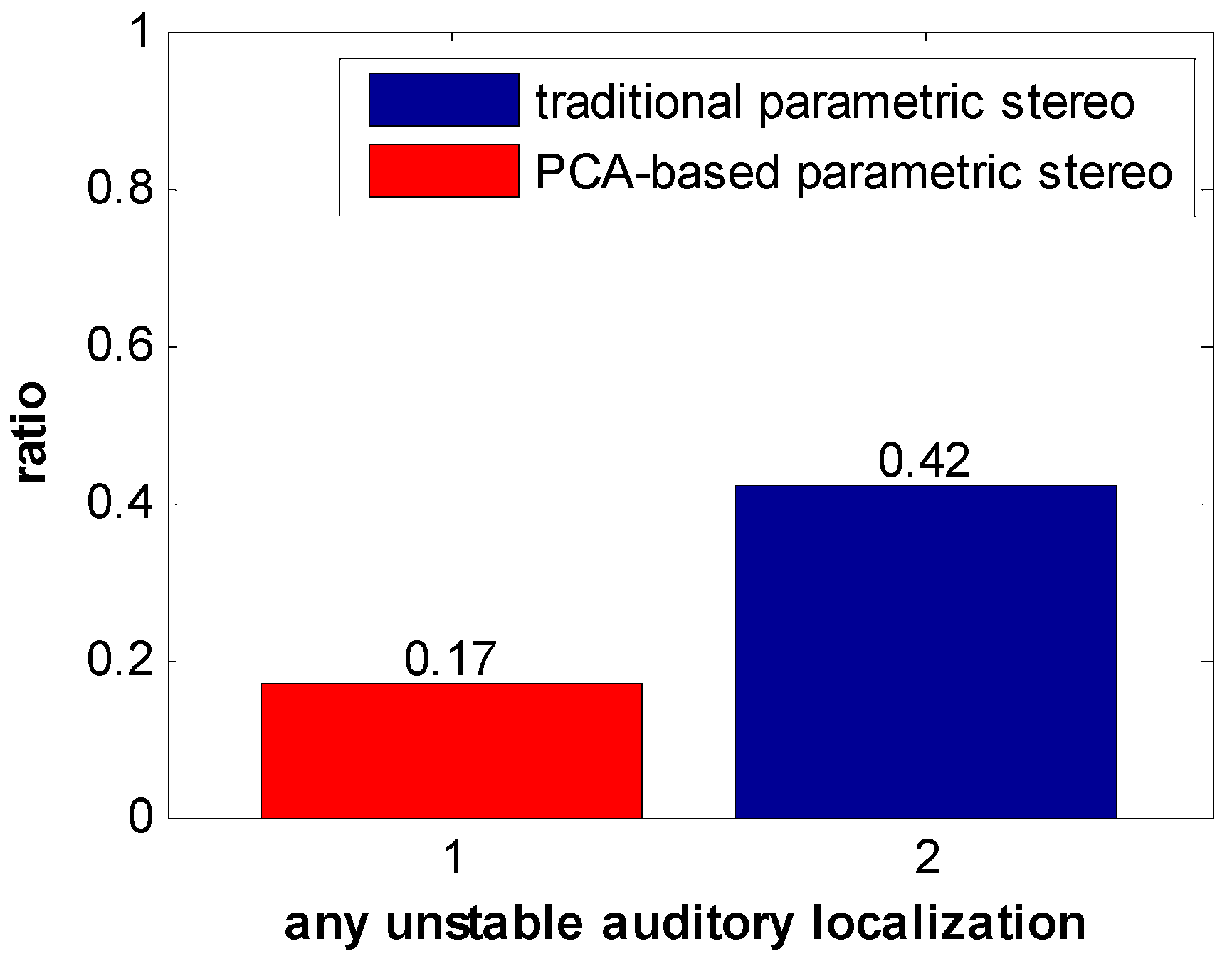
Figure 16 shows the results of a 0–1 test for spatial sense. In this test, 12 stereo music from EBU test materials is chosen. Score 0 means the sound localization is stable, and score 1 means there are some unstable sound localization in test materials. The ratio in Figure 16 is calculated from the times of unstable localization, and lower ratio means better performance in the quality of spatial sense. Experiments show that compared with the traditional parametric stereo encoding method, the spatial sense of the audio source has been obviously improved through the PCA-based parametric stereo. Through the use of PCA, almost half of the amount of parameter estimation can be reduced, while the computational complexity still rises because of the increasing complexity of PCA.

5. Test and Results

The method proposed in this paper performs significantly better with stereo signals compared to mono signals. Thus, this section only presents the results for stereo signals. In order to verify the encoding and decoding performance of the PCA-based stereo coding method, some optimized modules such as DTX, noise shaping, and other efficient coding tools in the codec were not used in testing

5.1. Design of Test Based on MUSHRA

The key points of the MUSHRA [25] test are as follows:

5.1.1. Test Material

(i) Several typical EBU test sequences were selected: piano, trombone, percussion, vocals, song of rock, multi sound source background and mixed voice, and so on.

(ii) Contrast test objects: PCA-based codec signal that transmits two channels separately, PCA-based codec signal with traditional parametric stereo, PCA-based codec signal with improved parametric stereo, G719 codec signal with traditional parametric stereo [24], HE-AACv2 codec signal, anchor signal, and original signal. In the algorithm proposed in this paper, the relationship between the quality of the restored signal and bitrate is not linear, as Figure 17 shows, which uses a simple subjective test with different bitrate allocation; therefore, the test chooses a case in which the qualities of restored signal and bitrate are both acceptable.

The bits allocations of each module in PCA–based codec for stereo signal are shown in

Table 7. Bitrate allocation in encoder.

Module	Bitrate
Reduced-dimensional matrix	35 kbps
Rotation matrix	5 kbps
First principal component	10 kbps
Spatial parameters and side information	5 kbps

.

(iii) In order to eliminate psychological effects, the order and the name of each test material in each group are random. The listener needs to select the original signal from the test signals and score 100 points, and the rest of the signals are scored by 0–100 according to overall quality, including sound quality and the spatial reduction degree.

5.1.2. Listeners

10 people with certain listening experiences were selected for the listening test, of which 5 were male, 5 were female, and each listener has normal hearing.

5.1.3. Auditory Environment

All 10 listeners use headphones connected to a laptop in quiet environments.

5.2. Test Results

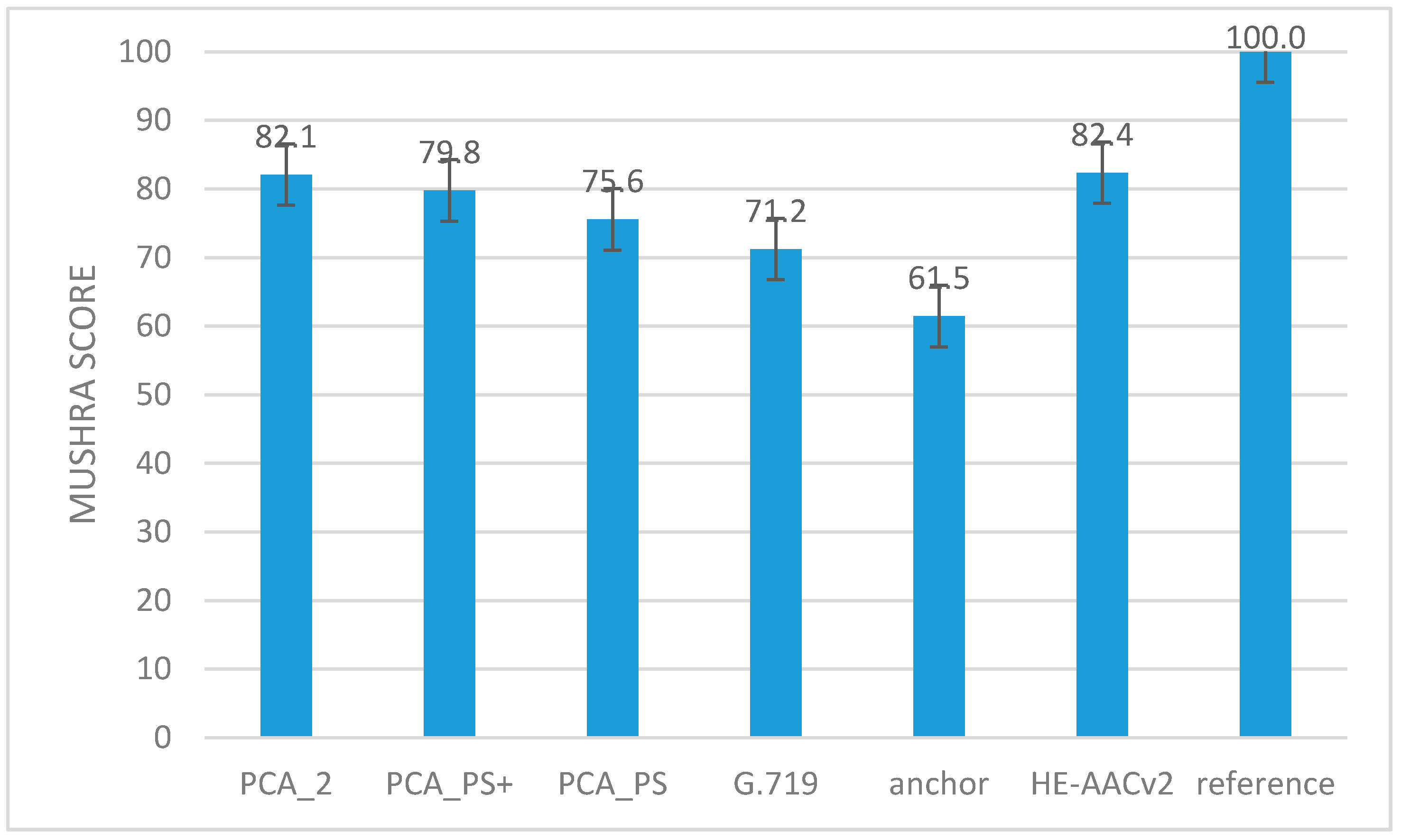
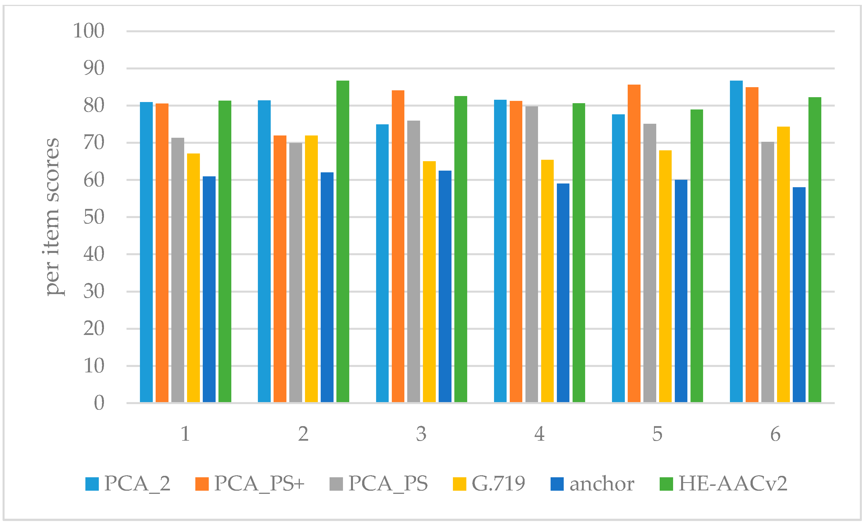
After the test is finished, we calculated average value and the 95% confidence interval based on the listeners’ scores. The average confidence interval of each test codec is [77.2, 87.0], [74.4, 84.2], [70.5, 80.7], [65.8, 76.6], [56.1, 66.9], and [78.6, 86.2]. After removing three outlier data (data beyond confidence interval), the test results of MUSHRA are shown in Figure 18 and Figure 19.

Compared with traditional parametric stereo, the PCA-based parametric stereo has less bitrate, higher quality, and better spatial sense. Compared with G719 with traditional parametric stereo with the same bitrate, PCA-based codec signal has better quality. Compared with HE-AACv2 signal, the average score of the PCA-based parametric stereo is slightly less than HE-AACv2. HE-AACv2 is a mature codec that uses several techniques to improve the quality, including Quadrature Mirror Filter (QMF), Spectral Band Replication (SBR), noise shaping and so on. The complexity of PCA is less than the part of the 32-band QMF in HE-AACv2. Considering the high complexity and maturity of HE-AACv2, the test results are optimistic. Conclusions can be drawn that the PCA-based codec method possesses good performance, especially for stereo signal in which the audio quality and spatial sense can be recovered well.

5.3. Complexity Analysis

The module of principal component analysis can be regarded as a part of the singular value decomposition (SVD): the calculate procession of the right singular matrix and the singular value of original matrix $X_{\left[\begin{array}{cc}m& n\end{array}\right]}$, therefore the algorithm complexity of principal component analysis module is O(n^3). According to the properties of SVD, when n < m, the computation complexity of the right singular matrix is half of the computation complexity of SVD for $X_{\left[\begin{array}{cc}m& n\end{array}\right]}.$ Therefore, the algorithm complexity and delay of PCA are far less than those of SVD. In the Intel i5-5200U processor, 4 GB memory, 2.2 GHz work memory, it takes 20 ms to finish one part of PCA. Given the time reduction of parametric stereo, the delay of PCA-based codec algorithm is in the acceptable range. In the part of multi-frame joint PCA, the forming of the original matrix takes 40 ms. When the first frame finishes MDCT, the process of forming original matrix will begin. Besides, the thread of PCA is different from matrix construction, and MDCT windowing also belongs to the calculating thread. Suppose the time for MDCT of first frame is t₁; the whole delay can be regarded as around 40 + t₁ ms, which is around 50 ms. The delay of the algorithm proposed in this paper still has space to be improved, and we can make the balance of delay and bitrate better by adjusting the number of multi frames using a more intelligent strategy in the future.

6. Discussion

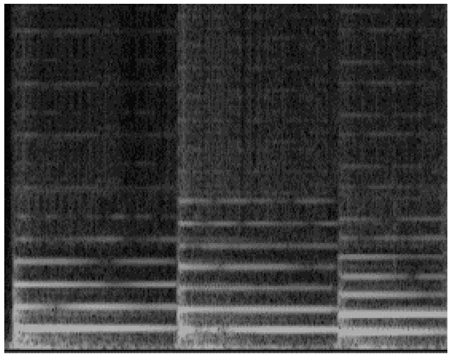
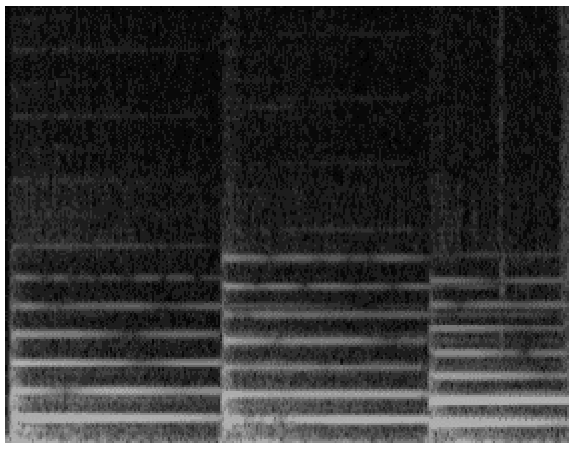
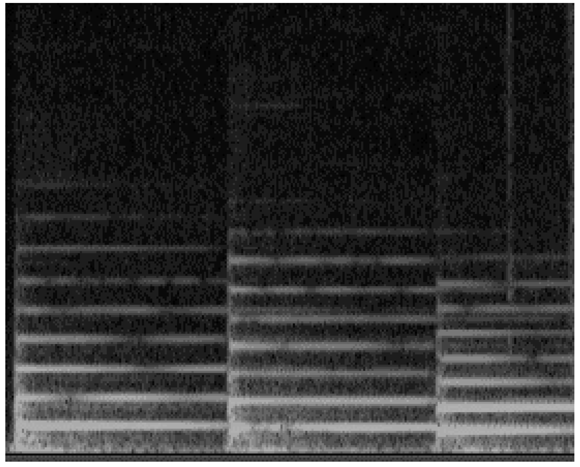
This paper just presents a preliminary algorithm. There is still much space for improvement in real applications. One question worth further study is how to eliminate the noise. In the experiment, when the number of bits or the number of principal components is too small, the noise spectrum has special nature, as Figure 20, Figure 21 and Figure 22 show. Signal in Figure 20 is restored by three components; compared with signal in Figure 21 and Figure 22, the spectrum of noise in high-frequency domain has obvious repeatability, which occurs once every 1.6 kHz. Therefore, low pass filter mentioned in Section 3.3 is not the best way to get rid of this noise: the damage of original signal is unavoidable. Ideally, an adaptive notch filter can filter the spectrum of noise clearly and not damage original signal. However, the design of such an adaptive notch filter needs to be studied more in the future.

7. Conclusions

The framework of proposed multi-frame PCA-based audio coding method has several differences compared to other codecs; therefore, there are lots of barriers to the design of an optimal algorithm. This paper proposed several ways to remove those barriers. For mono signal, the design of PCA-based coding method in this paper, including multi-frame signal processing, matrix design, and quantization design can hold it efficiently. As to stereo signal, PCA has high associativity with parametric stereo, which makes PCA-based parametric stereo certainly feasible and significant. Experimental results show satisfactory performance of the multi-frame PCA-based stereo audio coding method compared with the traditional audio codec.

In summary, research on the multi-frame PCA-based codec, both for mono and stereo, has certain significance and needs further improvement. This kind of stereo audio coding method has good performance in processing different kinds of audio signals, but further studies are still needed before it can be widely applied.

References

- Bosi, M.; Goldberg, R.E. Introduction to Digital Audio Coding and Standards; Kluwer Academic Publishers: Dordrecht, The Netherlands, 2003; pp. 399–400. ISBN 1402073577. [Google Scholar]
- Fatus, B. Parametric Coding for Spatial Audio. Master’s Thesis, KTH, Stockholm, Sweden, 2015. [Google Scholar]
- Faller, C. Parametric joint-coding of audio sources. In Proceedings of the AES 120th Convention, Paris, France, 20–23 May 2016. [Google Scholar]
- Blauert, J. Spatial Hearing: The Psychophysics of Human Sound Localization; MIT Press: Cambridge, MA, USA, 1983; pp. 926–927. ISBN 0262021900. [Google Scholar]
- ISO/IEC. 13818-7: Information Technology—Generic Coding of Moving Pictures and Associated Audio Information—Art 7: Advanced Audio Coding (AAC); ISO/IEC JTC 1/SC 29: Klagenfurt, Austria, 2006. [Google Scholar]
- Herre, J. From Joint Stereo to Spatial Audio Coding—Recent Progress and Standardization. In Proceedings of the 7th International Conference of Digital Audio Effects (DAFx), Naples, Italy, 5–8 October 2004. [Google Scholar]
- Jannesari, A.; Huda, Z.U.; Atr, R.; Li, Z.; Wolf, F. Parallelizing Audio Analysis Applications—A Case Study. In Proceedings of the 39th International Conference on Software Engineering: Software Engineering Education and Training Track (ICSE-SEET), Buenos Aires, Argentina, 20–28 May 2017; pp. 57–66. [Google Scholar]
- ISO/IEC. 14496-3:2001/Amd 2: Parametric Coding for High-Quality Audio; ISO/IEC JTC 1/SC 29: Redmond, WA, USA, 2004. [Google Scholar]
- Breebaart, J.; Par, S.V.D.; Kohlrausch, A.; Schuijers, E. Parametric coding of stereo audio. EURASIP J. Appl. Signal Process. 2005, 9, 1305–1322. [Google Scholar] [CrossRef]
- Faller, C.; Baumgarte, F.D. Binaural cue coding—Part I: Psychoacoustic fundamentals and design principles. IEEE Trans. Speech Audio Process. 2003, 11, 509–519. [Google Scholar] [CrossRef]
- Faller, C.; Baumgarte, F.D. Binaural cue coding—Part II: Schemes and applications. IEEE Trans. Speech Audio Process. 2003, 11, 520–531. [Google Scholar] [CrossRef]
- Zhang, S.H.; Dou, W.B; Lu, M. Maximal Coherence Rotation for Stereo Coding. In Proceedings of the 2010 IEEE International conference on multimedia & Expo (ICME), Suntec City, Singapore, 19–23 July 2010; pp. 1097–1101. [Google Scholar]
- Ahmed, N.; Natarajan, T.; Rao, K.R. Discrete cosine transform. IEEE Trans. Comput. 1974, 1, 90–93. [Google Scholar] [CrossRef]
- Smith, S.W. The Scientist and Engineer's Guide to Digital Signal Processing, 2nd ed.; California Technical Publishing: San Diego, CA, USA, 1997; ISBN 0-9660176. [Google Scholar]
- Skodras, A.; Christopoulos, C.; Ebrahimi, T. The jpeg 2000 still image compression standard. IEEE Signal Process. Mag. 2001, 18, 36–58. [Google Scholar] [CrossRef]
- Pearson, K. On Lines and Planes of Closest Fit to Systems of Points in Space. Philos. Mag. 1901, 2, 559–572. [Google Scholar] [CrossRef]
- Jia, M.S.; Bao, C.C.; Liu, X.; Li, R. A novel super-wideband embedded speech and audio codec based on ITU-T Recommendation G.729.1. In Proceedings of the 2009 Annual Summit and Conference of Asia-Pacific Signal and Information Processing Association (APSIPA ASC), Sapporo, Japan, 4–7 October 2009; pp. 522–525. [Google Scholar]
- Jia, M.S.; Bao, C.C.; Liu, X.; Li, X.M.; Li, R.W. An embedded stereo speech and audio coding method based on principal component analysis. In Proceedings of the International Symposium on Signal Processing and Information Technology (ISSPIT), Bilbao, Spain, 14–17 December 2011; Volume 42, pp. 321–325. [Google Scholar]
- Briand, M.; Virette, D.; Martin, N. Parametric representation of multichannel audio based on Principal Component Analysis. In Proceedings of the 120th Convention Audio Engineering Society Convention, Paris, France, 1–4 May 2006. [Google Scholar]
- Goodwin, M. Primary-Ambient Signal Decomposition and Vector-Based Localization for Spatial Audio Coding and Enhancement. In Proceedings of the IEEE Conference on Acoustics, Speech, and Signal Processing (ICASSP), Honolulu, HI, USA, 15–20 April 2007; pp. I:9–I:12. [Google Scholar]
- Chen, S.X.; Xiong, N.; Park, J.H.; Chen, M.; Hu, R. Spatial parameters for audio coding: MDCT domain analysis and synthesis. Multimed. Tools Appl. 2010, 48, 225–246. [Google Scholar] [CrossRef]
- Robert, C.S.; Stefan, W.; David, S.H. Mean opinion score (MOS) revisited: Methods and applications, limitations and alternatives. Multimed. Syst. 2016, 22, 213–227. [Google Scholar] [CrossRef]
- Hou, Y.; Wang, J. Mixture Laplace distribution speech model research. Comput. Eng. Appl. 2014, 50, 202–205. [Google Scholar] [CrossRef]
- Jiang, W.J.; Wang, J.; Zhao, Y.; Liu, B.G.; Ji, X. Multi-channel audio compression method based on ITU-T G.719 codec. In Proceedings of the Ninth International Conference on Intelligent Information Hiding and Multimedia Signal Processing (IINMSP), Beijing, China, 8 July 2014. [Google Scholar]
- ITU-R. BS.1534: Method for the Subjective Assessment of Intermediate Quality Level of Coding Systems; International Telecommunication Union: Geneva, Switzerland, 2001. [Google Scholar]
Figure 1.
Flowchart of mono encoder. (TF, Time-to-Frequency; PCA, Principle Component Analysis).
Figure 2.
Flowchart of mono decoder. (iPCA, inverse Principle Component Analysis; FT, Frequency-to-Time).
Figure 3.
Scheme of PCA-based coding method. (PCA, Principle Component Analysis).
Figure 4.
Compression rate for different format of matrix.
Figure 5.
Example for matrix construction (“value” means the value of cells in original matrix, “column” means the column of original matrix, and “row” means the row of original matrix).
Figure 6.
Subjective test results for different number of frames.
Figure 7.
Multi-frame in encoder. (PCA, Principle Component Analysis; Rd, reduced-dimensional).
Figure 8.
Multi-frame in decoder. (iPCA, inverse Principle Component Analysis; Rd, reduced-dimensional).
Figure 9.
Bits allocation for reduced-dimensional matrix (darker color means more bits needed).
Figure 10.
An example rotation matrix (“value” means the average value of cells in rotation matrices, “column” means the column of rotation matrix, and “row” means the row of rotation matrix).
Figure 11.
Bit allocation for rotation matrix (darker color means more bits needed; white color means no bits).
Figure 12.
Flowchart of stereo encoder. (MDCT, Modified Discrete Cosine Transform; PCA, Principle Component Analysis; IC, Interaural Coherence; ILD, Interaural Level Difference).
Figure 13.
Flowchart of stereo decoder. (MDCT, Modified Discrete Cosine Transform; iPCA, inverse Principle Component Analysis; IC, Interaural Coherence; ILD, Interaural Level Difference).
Figure 14.
Subjective MOS of high-relation stereo signal. (MOS, Mean Opinion Score).
Figure 15.
Subjective MOS of low-relation stereo signal.
Figure 16.
Test results for spatial sense.
Figure 17.
Relationship between quality and bitrate.
Figure 18.
Results of MUSHRA test. (PCA_2 represents the PCA-based codec signal that is transmitted over two channels separately (75 kbps), PCA_PS+ represents PCA-based codec signal with improved parametric stereo (55 kbps), PCA_PS represents PCA-based codec signal with traditional parametric stereo (56 kbps), G.719 represents G.719 codec signal with traditional parametric stereo (56 kbps), anchor represents anchor signal, HE_AACv2 represents HE-AACv2 signal (55 kbps), and reference represents hidden reference signal).
Figure 19.
MUSHRA score of per item test. (PCA_2 represents the PCA-based codec signal that is transmitted over two channels separately (75 kbps), PCA_PS+ represents PCA-based codec signal with improved parametric stereo (55 kbps), PCA_PS represents PCA-based codec signal with traditional parametric stereo (56 kbps), G.719 represents G.719 codec signal with traditional parametric stereo (56 kbps), anchor represents anchor signal; HE-AACv2 represents HE-AACv2 signal (55 kbps), and hidden reference material has been removed. 1–6 represents different test materials).
Figure 20.
The spectrogram of the signal restored by three components.
Figure 21.
The spectrogram of the signal restored by four components.
Figure 22.
The spectrogram of the signal restored by five components.