Using the Partial Wave Method for Wave Structure Calculation and the Conceptual Interpretation of Elastodynamic Guided Waves

Department of Engineering Science and Mechanics, Pennsylvania State University, University Park, PA 16802, USA
*
Author to whom correspondence should be addressed.
Appl. Sci. 2018, 8(6), 966; https://doi.org/10.3390/app8060966
Submission received: 8 May 2018
/
Revised: 1 June 2018
/
Accepted: 8 June 2018
/
Published: 12 June 2018
(This article belongs to the Special Issue Ultrasonic Guided Waves)
Abstract
:Featured Application
Shortcut to wave-structure calculation for elastodynamic guided waves and prediction of acoustic leakage behavior.
Abstract
The partial-wave method takes advantage of the Christoffel equation’s generality to represent waves within a waveguide. More specifically, the partial-wave method is well known for its usefulness when calculating dispersion curves for multilayered and/or anisotropic plates. That is, it is a vital component of the transfer-matrix method and the global-matrix method, which are used for dispersion curve calculation. The literature suggests that the method is also exceptionally useful for conceptual interpretation, but gives very few examples or instruction on how this can be done. In this paper, we expand on this topic of conceptual interpretation by addressing Rayleigh waves, Stoneley waves, shear horizontal waves, and Lamb waves. We demonstrate that all of these guided waves can be described using the partial-wave method, which establishes a common foundation on which many elastodynamic guided waves can be compared, translated, and interpreted. For Lamb waves specifically, we identify the characteristics of guided wave modes that have not been formally discussed in the literature. Additionally, we use what is demonstrated in the body of the paper to investigate the leaky characteristics of Lamb waves, which eventually leads to finding a correlation between oblique bulk wave propagation in the waveguide and the transmission amplitude ratios found in the literature.
1. Introduction
In this paper, we demonstrate how the partial-wave method, as first introduced by Solie and Auld [1], can be used to gain a new perspective on guided waves. This new perspective adds to our understanding of the structure of guided waves, and provides valuable insight into the leaky characteristics of Lamb waves (which are not to be confused with the study of leaky Lamb waves and their corresponding dispersion curve solutions).
At present, our understanding of guided waves is primarily informed by the derivation of characteristic equations and dispersion curve solutions. The dispersion curve solutions in particular have become significantly more accessible with the widespread use of the semi-analytical finite element (SAFE) method. However, the SAFE method does not provide the same level of understanding that would be possible by analyzing a characteristic equation. The most well-known example of this is that the two-part Lamb wave characteristic equation shows that all of the Lamb waves can be divided into two types: symmetric and anti-symmetric. Hence, the importance of the present work. However, this paper will not cover the calculation of dispersion curves, attenuation, energy loss, or anisotropic materials. Neither will it cover the derivation of characteristic equations for various guided waves.
For the purpose of clarity, in this paper, bulk waves are plane waves that travel through the bulk of a media, and surface waves are plane waves that travel along the surface of a media. It is emphasized that all of the waves are considered to have a planar wavefront.
Section 2 and Section 3 will provide a brief history and the fundamentals of the partial-wave method and the Christoffel equation, respectively. These sections give special attention to the diction used and the assumptions made, as they are pertinent to how the interpretation presented in this paper deviates from the literature. Section 4 describes this new method of interpretation. It discusses in detail how the slowness curve solutions of the Christoffel equation can be used to interpret the characteristics of most guided waves, and the Lamb wave solutions in particular. Section 5 and Section 6 apply the new method of interpretation to a variety of guided waves, which include Rayleigh waves, Stoneley waves, Lamb waves, and shear horizontal waves.
Section 7 focuses on Lamb waves, and a method developed in Section 6 is used to investigate the contributions of each partial wave to Lamb waves from 50 kHz to 20 MHz for a 1-mm thick aluminum plate. This section also identifies characteristics of Lamb waves that have not been formally discussed in the literature.
Section 8 uses the results from the previous sections to develop an understanding of the leaky characteristics of Lamb waves. Various characteristics of the acoustic leakage from the waveguide can be easily determined, including the angle of propagation and the amplitude of emission based on the interface conditions. A correlation between the amount of acoustic leakage and the refraction qualities of obliquely travelling bulk waves in the guided wave is also identified.
2. The Partial Wave Method
The term ‘partial-wave method’ first appeared in a paper by Solie and Auld in 1973 [1]; specifically, it was called “the method of partial waves (or transverse resonance)”. This method was described as follows: “In this method, the plate wave solutions are constructed from simple exponential-type waves (partial waves), which reflect back and forth between the boundaries of the plates…” They go on to write, “A basic principle of the partial wave method is that the partial waves are coupled to each other by reflections at the plate boundaries”.
In Auld’s 1990 monograph [2], he discusses the method further: “[the superposition of partial waves method] can be further simplified by making use of the transverse resonance principle, which has been used to great advantage in electromagnetism” [emphasis added by Auld]. That is, what is known colloquially as the partial-wave method can be broken down into two parts. First, there is the superposition of the partial-waves method, which uses the principle of superposition with the Christoffel equation’s solutions (i.e., partial waves) [2]. Second, there is the transverse resonance principle, which assumes that the standing wave perpendicular to wave propagation can only exist if the partial waves satisfy the relevant boundary conditions [2,3]. Modern application of the partial-wave method includes the calculation of dispersion curves using the global-matrix method or the transfer-matrix method for anisotropic plates and/or multilayered plates [4,5].
3. The Christoffel Equation and the Use of Slowness Curves
The Christoffel equation is critical to the flexibility and strength of the partial-wave method. The Christoffel equation can be derived by assuming a plane wave (Equation (4)) propagating in a solid elastic media (Equations (1)–(3)).
Here , , and are the stress, strain, and displacement; and are the mass density and elastic stiffness; and are the wave vector and angular frequency; , and is the time variable. When combined, Equations (1)–(4) yield the Christoffel equation:
When Equation (5) is solved, a slowness curve/surface can be calculated and plotted in an inverse phase velocity space.
3.1. Deriving the Expression for the Slowness Curves of an Isotropic Solid
For an isotropic linear elastic solid, Equation (2) can be replaced with:
where and are the Lamé parameters and is the Kronecker delta. As a side note, in addition to replacing Equation (2) with Equation (6), if Equation (4) is replaced with:
or:
then, the Christoffel equation can be used to derive the relationship between the Lamé parameters, the longitudinal wave speed, , and the shear wave speed, :
where and are the unit vectors along the -axis and the -axis. Using Equation (6), assuming (i.e., wave propagation in the – plane), and dividing through by , Equation (5) can be rearranged into matrix form:
where:
Equations (11) and (12) represent a system of linear homogeneous equations, where and = . The non-trivial solution to Equation (11) only exists if:
Expanding Equation (13) based on Equation (12) results in:
The solutions to the characteristic equation (Equation (14)) are:
If Equations (9) and (10) are considered, the right-hand side of Equations (15) and (16) become and , respectively. These represent the slowness curve solutions to the Christoffel equation of an isotropic material. It should be noted that in Equation (14), the squared term represents the multiplicity in the shear wave’s slowness curve solutions.
3.2. Interpretation of Slowness Curve Solutions
From the previous section, it is clear that the solutions to the Christoffel equation do not take into consideration the boundary conditions (BCs) of the problem. That is, the solution only depends on the material properties of the elastic solid in which the plane waves propagate. As a result, in the literature, it is shown that the Christoffel equation can be used to determine the reflection and refraction characteristics of plane waves at oblique incidence to an interface between anisotropic elastic solids [6,7,8]. Additionally, the energy velocity vector and the bulk wave’s skew angle can be calculated [4].
Slowness curves are often plotted in terms of the ‘inverse phase velocity’. However, since phase velocity is not a vector, the use of the term ‘inverse phase velocity’ to describe the slowness vector can be confusing. A different notation that may be easier to conceptually understand is plotting slowness curves on the and axis instead of the versus axis. Therefore, if a ray is drawn from the origin to a point on the slowness curve, it is understood that its unit vector describes the wave propagation direction in the – plane.
Since the focus of the partial-wave method is on guided waves, for the purposes of this paper, it is assumed that the wave is propagating parallel to the boundary/interface, which we take to be in the -direction. The -axis is through the thickness of the elastic solid. This coordinate system will be maintained throughout the entirety of the paper, with additional details depending on the problem being considered. Further, continuing to assume that , and using the frequency–wavenumber (-) pairs obtained from any one of the many methods for calculating dispersion curves (i.e., enforcing the BC and solving the eigenvalue problem), the Christoffel equation becomes a complex valued quadratic eigenvalue problem in three dimensions. The solution, should it exist, will always be composed of six complex valued eigensolutions. These six solutions are the partial waves of the partial-wave method. The partial waves can be paired up into three pairs, and each pair is composed of an upward and a downward propagating wave (i.e., the magnitudes of the eigenvalues are the same, but the signs are opposite) [1,4].
In Auld [2], there is a discussion of regions for an increasing , in which the partial waves have specific characteristics. Also, in Auld [2], it is recognized that at an interface, is the same for all of the partial waves in order to satisfy Snell’s law, and that a given guided wave must theoretically have a single value for a given . Auld gives an example for an isotropic material, which has two slowness curves and three regions (see Equations (15) and (16)):
The inverses of the shear and longitudinal group velocities ( and ) are also the radii of the two slowness curves, which are circles for an isotropic material. By Crandall’s paper [6], it is also understood that outside of these circles, the value for becomes imaginary, and the magnitude traces a hyperbola.
Auld also gives examples of slowness curve representations for a shear horizontal (SH) mode composed of obliquely travelling bulk waves, and a piezoelectric plate with leaky electromagnetic radiation [2].
This concludes the state-of-the-art section of the paper. How these theories and concepts allow us to reinterpret our understanding of guided waves in a novel way is discussed from here onward.
4. Reinterpreting the Dispersion Curves
As mentioned previously, the Christoffel equation is only dependent upon the material properties of the elastic solid in which the plane waves propagate. The BCs are not used until the partial-wave method is applied. Not only that, but the boundary conditions are not limited to the conventional traction-free BCs (e.g., Lamb waves). As a result, the partial-wave method is not limited to any specific type of waveguide. In fact, most types of guided waves should be representable using slowness curves. For some, such as the shear horizontal guided waves, this approach is more cumbersome than the standard derivation. However, its value lies in how it provides a fundamental foundation for all of the guided waves, and a common method for interpreting and comparing each one. When considering reflection/transmission, mode conversion, or multi-mode propagation, this perspective is quite beneficial.
In modern literature, perhaps the most commonly used dispersion curves are of Lamb waves in an aluminum plate in terms of phase velocity versus the frequency–thickness product. Using the three regions depicted in Figure 1, we can divide the phase velocity dispersion curves into three regions, as shown in Figure 2. By doing this, it is possible to view how the dispersion curve solutions match up with the partial waves’ characteristics. For example, this is a good way to dispel the potential misconception that guided waves are composed of multiple reflecting bulk waves. That is, the original assumption of plane wave propagation (Equation (4)), which is fundamental to the Christoffel equation, does not exclude the surface wave solution (i.e., imaginary-valued ) as increases. It would be more accurate to say that guided waves are a superposition of reflecting bulk waves and surface waves with elliptical particle motion (this will be shown in the later calculations and examples).
In fact, guided waves composed solely of reflecting bulk waves exist only in Region 3 (c), where they are highly dispersive. However, there is one exception to this rule: there exists a range of phase velocities in Region 2 (Figure 1b), where only bulk waves propagate, which will be discussed in a later section.
The A0 mode and Rayleigh waves exist in Region 1 (Figure 1a), where each guided wave can be represented in terms of six surface waves. The low-frequency S0 mode is in Region 2 (b), and is composed of two surface waves and two bulk waves (as will be shown later in the paper), excluding the two shear horizontal partial waves.
The line separating Region 1 (Figure 1a) and Region 2 (Figure 1b) has great significance, since many Lamb wave modes appear nearly non-dispersive near it. That is, the higher-order Lamb waves approach the shear wave speed, and the A0 and S0 modes approach the Rayleigh wave speed for large values. The shear horizontal modes also converge to this line for large values. The line separating Region 2 (Figure 1b) and Region 3 (Figure 1c) has many higher-order Lamb modes, which appear nearly non-dispersive close to it as well.
The A0 and S0 Lamb wave modes’ tendency to approach the Rayleigh wave phase velocity can also be explained using this reinterpretation, since increasing will increase the magnitude of the imaginary-valued (see Figure 1a). Once increases sufficiently, the surface waves decay with the depth from the surface before interacting with the opposite traction-free boundary, thereby imitating a Rayleigh wave. This also explains why quasi-Rayleigh waves [9] have similar wave structures to Rayleigh waves. That is, the quasi-Rayleigh wave and the Rayleigh wave are both composed of partial waves (with slight differences in amplitude and exponential decay).
Many higher-order Lamb modes have wave structures that are sinusoidal through the thickness, but have slightly larger or smaller amplitudes near the traction-free boundaries. In Region 2 (Figure 1b), this could be explained by surface waves affecting the wave structure near the traction-free boundaries, while the reflecting bulk waves create the sinusoidal appearance.
This reinterpretation of guided waves provides for the relatively simple calculation of wave structures based on the superposition of the partial-wave eigensolutions. Based on the preceding concepts and with wave propagation in the -direction, . Solving Equations (15) and (16) for results in:
and:
respectively. Equations (9), (10) and (17) can then be substituted into Equation (11) to get matrix as a function of and :
And Equations (9), (10) and (18) can be substituted into Equation (11) to get matrix as a function of and and :
Finding the reduced row echelon form of and gives the solution to the eigenvectors, which contain, at most, two free variables (i.e., and ). Considering and , and also the “” terms in them, which correspond with the sign of , results in four possible eigenvectors (not including the multiplicity). For the positive eigenvalue of the longitudinal wave, the eigenvector is:
While for the negative eigenvalue of the longitudinal wave, the eigenvector is:
For the positive eigenvalue of the shear wave, the eigenvector is:
While for the shear wave’s negative eigenvalue, the eigenvector is:
The superscripts and correspond to the longitudinal and the shear waves, respectively. The can be made more specific by using and to denote the shear vertical and shear horizontal polarizations.
Examining Equations (21) and (22), it is clear that for , the square root becomes imaginary-valued, and for , the square-root becomes real-valued. These two scenarios correspond with the surface wave and bulk wave solutions, respectively. The same holds true for Equations (23) and (24) with instead of , with p = 0. For or and positive , the corresponding eigenvector is:
and for negative it is:
Hence, for very large values (relative to their respective wave speeds), the eigenvectors become circularly polarized, regardless of whether it is a shear wave or longitudinal wave. Lastly, for a given and , the values of the four partial waves (not including the multiplicity of the shear waves) can be calculated using Equations (15) and (16):
As implied previously, since the solution of the Christoffel equation does not depend on the boundary/interface conditions, a linear combination of the partial waves should be able to represent most elastodynamic guided waves, regardless of the boundary/interface conditions. We demonstrate this in the following sections. The material properties shown in Table 1 will be used. For each partial-wave eigenvector calculated in the following examples, the free variable is set equal to unity; then, the resulting eigenvector is normalized into a unit vector by dividing by its magnitude.
5. Rayleigh Waves and Generalized Rayleigh Waves
5.1. Rayleigh Waves
The Rayleigh wave, which travels at the surface of a half-space, is a good starting example, since its solution is well-known, and this different approach will mirror the conventional derivation in the literature. The term ‘generalized Rayleigh waves’ will be used to refer to a class of wave propagation solutions developed following the original Rayleigh wave derivation, as was done by Stoneley [11]. This will be considered later in section V.B.
Assuming an aluminum half-space with the boundary at , an example Rayleigh wave calculation is completed using the previously mentioned methods. The eigensolutions for the six partial waves at a frequency of rad/s and a wavenumber of 1103.4 rad/m are shown in Table 2. The frequency and wavenumber were chosen to match the non-dispersive phase velocity solution to the standard Rayleigh wave problem.
There are several notable results in Table 2:
- All of the values are imaginary, since Rayleigh waves exist in Region 1 (Figure 1a);
- is larger in magnitude than and because of the hyperbolic shape of the imaginary-valued slowness curves;
- , , , and have a multiplicity due to the isotropic material properties;
- The eigenvectors are complex, which suggests elliptical particle motion [9];
- and are not complex-valued.
As shown in Figure 3, only the exponentially decaying solutions are necessary for the Rayleigh wave solution, because the domain is a half-space.
Although the derivation method is different, closer inspection of the solutions shows that they match the values of and given by Viktorov [9]. In the conventional derivation, the Rayleigh wave solution is a superposition of two exponentially decaying terms that are dependent upon the phase velocity and material properties, so this close agreement is expected. A superposition of the two partial waves, when , can be represented as:
The amplitudes of each partial wave, and , are solved for by substituting into one of the BCs:
and assuming . This approach is taken in lieu of satisfying both BCs (by setting the determinant of the coefficients matrix equal to zero), since is an approximate value, and the determinant is never exactly zero, so most attempts at getting a reduced row echelon form of the matrix result in the trivial solution of the eigenvector. To avoid this dilemma, we set , and normalized as necessary. could be used in place of the other BC, but only one is necessary. Solving for , it is found that . Plotting Equation (29) with the calculated values of and gives the same wave structure for a Rayleigh wave as that found in Viktorov [9].
5.2. Stoneley Waves
The same approach can be applied to generalized Rayleigh waves. Generalized Rayleigh waves refer to guided waves that demonstrate Rayleigh wave-like characteristics, such as for example, Stoneley waves, Scholte waves, and Love waves [11,12,13]. For this example, Stoneley waves will be the focus, but a similar approach can be applied to the others as well.
Stoneley waves, which propagate along the interface between two half-spaces, will be analyzed as an example. Stoneley waves typically have a non-dispersive phase velocity that is slightly less than the denser material’s bulk shear wave velocity, which means that it is in Region 1 (Figure 1a). A Rayleigh wave-like wave structure should exist in the denser half-space [2]. A tungsten half-space rigidly connected to an aluminum half-space will be used for the example. Using Auld’s example (i.e., on pages 104–105 in [2]), the six eigensolutions are calculated for a frequency of rad/s and a wavenumber of rad/m. The frequency and wavenumber are chosen to meet the non-dispersive phase velocity solution to the Stoneley wave problem [2]. The eigensolutions at this frequency and wavenumber are shown in Table 3 and Table 4 for tungsten and aluminum, respectively.
For both tungsten and aluminum, the Stoneley wave is in Region 1 (Figure 1a). To construct the Stoneley wave displacement solution, the following partial waves are needed: solutions and from aluminum’s Christoffel equation, and solutions and from the tungsten’s Christoffel equation. Solutions and from the aluminum are considered to be exponentially decaying solutions for + values, while solutions and from the tungsten are considered to be exponentially decaying solutions for − values. These are shown in Figure 4 with respect to the interface.
The superposition of partial waves for each material, when , is shown in Equations (32) and (33). For tungsten (using values from Table 3):
while for aluminum (using values from Table 4):
Since the two half-spaces are assumed to be welded at the interface, the three of the four available interface conditions:
can be used to solve for the amplitudes , , and (i.e., assuming ).
Using these interface conditions, it was found that , , . Equations (32) and (33) can now be plotted to get the Stoneley wave’s wave structure, as shown in Figure 5.
6. Lamb Waves and Shear Horizontal Waves
Consider a 1-mm thick aluminum plate with traction-free BCs, and the same frequency as was analyzed in the previous section. The wavenumbers are calculated based on the Lamb wave dispersion curve solutions at that frequency.
6.1. A0 Lamb Wave Mode
The six eigensolutions at a frequency of rad/s and a wavenumber of 1688.7 rad/m are shown in Table 5. This frequency–wavenumber pair corresponds with the red-triangle symbol plotted in the dispersion-curve plot shown in Figure 2. Similar to the Christoffel equation solutions used for the Rayleigh -wave case, the solutions in Table 5 are typical of Region 1 (Figure 1a), in which the A0 mode exists. Unlike the Rayleigh wave case, there is now a bottom surface, so the exponentially increasing eigensolutions are now necessary, although they will be written as exponentially decreasing from the bottom surface upward as . Using the coordinate system shown in Figure 6, assignment to the top or bottom of the plate means that the partial waves will be defined using or , respectively. For simplicity, the rule used in this paper to categorize the partial waves between the top or bottom of the plate is shown in Table 6.
The superposed displacement profile in the z-direction is constructed by considering the symmetry of the problem:
where . For partial waves existing on the bottom surface of the plate, it is shown in Equation (38) that the -position is offset by the thickness of the plate. Just as in the Rayleigh wave problem, , , and can be solved by using three of the four BC available (assuming that ):
It was found that , and . As before, Equation (38) can now be used to plot the wave-structure of the A0 mode at this frequency.
6.2. S0 Lamb Wave Mode
The six eigensolutions at a frequency of rad/s and a wavenumber of 591.57 rad/m are shown in Table 7, where the shear vertical solutions have real-valued and real-valued eigenvectors. This frequency–wavenumber pair corresponds with the red-diamond symbol plotted in the dispersion-curve plot shown in Figure 2. These solutions correspond with the bulk waves reflecting within the plate waveguide (see Figure 7).
The displacement solution is constructed in a manner analogous to the A0 mode, except now there are bulk waves present:
, and are determined by using three of the four BCs (Equations (39)–(42)) (assuming that ), and are found to be , and . As before, Equation (43) can now be used to plot the wave structure of the S0 mode at this frequency. Occasionally, the plotted wave structure will be at a phase that is inconsistent with the conventional wave structure figures. This can be corrected by multiplying all of the displacements by , where . This multiplication is equivalent to letting the wave propagate over some non-zero distance and/or time.
6.3. Shear Horizontal Guided Wave Mode
Since the shear horizontal (SH) guided wave modes are similar to each other, a single discussion of how each behaves is possible. The dispersion relationship found in Rose [4] is:
is the guided wave mode number, and . The phase velocity is equal to the shear wave velocity for , and for large values, it approaches the shear wave velocity for all . The shear wave velocity represents the boundary between regions 1 and 2 (Figure 1a,b). That is, and . The SH partial wave exists as a bulk wave in the plate that is propagating parallel to the traction-free boundaries. When and is not large, then the SH guided wave modes increase in phase velocity and are highly dispersive. With the increasing phase velocity, the incidence angles of the SH bulk waves decrease as the solution of the Christoffel equation traces the shear slowness curve (the slowness curve representation of this dispersive SH guided wave mode is shown in Auld [2]).
7. The Contribution of Various Partial Waves in Each Lamb Wave
7.1. Symmetry and Opposing Phases
Based on the results from the S0 and A0 Lamb wave examples, it would seem as if there is an inherent symmetry to the problem, since the amplitudes of the partial wave pairs often have equal magnitudes or are out of phase by 180°. This is due to the problem’s symmetric geometry. This leads to the following simplification to the displacement solution used to calculate the wave structure:
where is either +1 or −1. Determining which partial waves should be assigned to the top or bottom of the plate is done in the same way as in the previous examples. As before, it is still implied by the use of the Christoffel equation that . In practice though, a few test calculations reveal that although the amplitudes of the partial-wave pairs are close to equivalent, they are not exactly equivalent. At best, Equation (45) can be used as a general description of the characteristics of many of the Lamb waves, but it is not a mathematically viable solution for our current application. That being said, the general description is invaluable for analyzing the characteristics of Lamb waves.
7.2. Using Symmetry to Summarize the Contribution of Longitudinal and Shear Partial Waves
One of the advantages of the partial-wave method approach is that the contribution of each partial wave can be determined for each Lamb wave mode. That is, if the amplitudes are normalized by dividing by:
and since due to the symmetry of the problem, a representation of the amount of longitudinal partial wave contribution can be calculated using the average of and :
This average is used to account for the approximate nature of the solutions. is representative of the amount of the longitudinal partial waves that make up a given Lamb wave mode, and is overlaid on the dispersion curves as an intensity plot in Figure 8a.
Similarly, since due to the symmetry of the problem, the contribution of the shear vertical partial waves can also be shown by calculating:
and plotting it in Figure 8b.
In Figure 8, it can be seen that in Region 1 (Figure 1a), the apportionment of longitudinal (i.e., ) and shear vertical (i.e., ) partial waves are similar. However, in regions 2 and 3 (Figure 1b,c) however, this is no longer the case. In Region 2 (Figure 1b), the Lamb waves around 4000 m/s are almost entirely made up of bulk shear vertical partial waves, and Lamb waves just below 6000 m/s are made up of mostly surface longitudinal partial waves. Interestingly, Lamb modes have phase and group velocities of and are comprised of shear bulk waves propagating at ±45° [14]. Region 2 (Figure 1b) also has a clear phase velocity dependence on the amount of each partial wave, but no frequency dependence. In Region 3 (Figure 1c), a certain degree of mode dependence appears, but it does not appear to differentiate between symmetric and anti-symmetric modes.
7.3. Using Opposing Phases to Sort Symmetric and Anti-Symmetric Lamb Wave Modes
Another advantage of using the partial-wave method is that the phase difference between the partial waves at the top and bottom of the plate can be different depending on the type of Lamb wave. That is, in symmetric modes, the top partial wave will be about 180° out-of-phase with the bottom partial wave. Anti-symmetric modes will typically have the top and bottom partial waves in-phase. This can be demonstrated by calculating from Equation (45):
which should be equivalent to:
However, since the frequency–wavenumber pairs are approximations, will vary from to for most Lamb waves. The values of are overlaid on the dispersion curves in Figure 9. It is worth emphasizing that the phase difference between the top and bottom partial waves applies to both the longitudinal and shear vertical partial waves, as shown in Equation (45).
Figure 9 demonstrates the phase difference characteristics of symmetric and anti-symmetric Lamb waves, but it also shows how those characteristics break down at high frequencies where dispersion curves intersect. At these intersection points, a phase difference (either or ) will dominate the surrounding points of both dispersion curves. The clearest examples of this phenomenon are circled in red in Figure 9.
8. Leaky Characteristics of Lamb Waves
Lamb waves travel through a traction-free plate. Leaky Lamb waves are the waves that propagate through the same waveguide when the traction-free boundaries are replaced with fluid half-spaces. The theoretical literature on leaky Lamb waves focuses on the calculation of dispersion curves and determining how these curves differ from the conventional Lamb wave dispersion curves [15,16]. The focus of this section is not this, but rather the leaky characteristics of Lamb waves, assuming there is no change in the dispersion curves. That is, the dispersion curves of a plate surrounded by a vacuum will be used as an approximation for the dispersion curves of a plate surrounded by air. This is a universal standard practice. The goal will be to use the partial-wave method to determine the characteristics of the acoustic leakage into the fluid from the Lamb wave travelling in the plate waveguide.
Before continuing, it should be stated that for fluids, the Eulerian form of the balance of linear momentum for acoustics is:
This complicates the velocity–pressure relationship of the acoustic fluid. To simplify this, it is assumed that the displacement is time-harmonic, which makes the particle velocity:
It is also assumed that the displacement is spatially harmonic and longitudinal in polarization such that:
where is the unit vector denoting the direction of wave propagation. Using Equations (52) and (53) in Equation (51) results in:
The Eulerian form can approximate the Lagrangian form with these assumptions if:
Equation (55) can be rearranged to:
If it is assumed that the phase velocity is around m/s and that displacements are about m, then for frequencies much less than rad/s, the Eulerian form should approximate the Lagrangian form. As a result, the simpler pressure–velocity relationship:
which was derived from the Lagrangian form of the balance of linear momentum for fluids assuming a time-harmonic displacement, can be used for the following example.
As an acoustic wave in a fluid, the slowness curve can be plotted as a circle with a radius equal to . Plotted with respect to aluminum’s slowness curve, the order of magnitude difference in radii makes all but the very dispersive part of the A0 mode, at very low frequencies, emit acoustic bulk waves (see Figure 10). At these low frequencies, the A0 mode is highly dispersive, and has a phase velocity lower than the acoustic wave speed in air.
The comparison of slowness curves from various media, which are shown in Figure 10, is similar to an example in Auld [2], but that example discussed the electromagnetic emission from a piezoelectric waveguide. The approach relies on Snell’s law, dictating that the wavenumber (i.e., ) should be equal at the interface between media. However, if Snell’s law were to be used directly, complex-valued angles (i.e., ) would need to be used.
Based on this slowness curve representation, it can be concluded that the acoustic leakage will be an obliquely travelling bulk wave. The angle of incidence of the acoustic leakage would be between 0° and 20° for most Lamb waves. If these findings are applied to air-coupled transducers, it would suggest that there is an optimum angle of reception for the air-coupled transducers.
The partial waves for air can be represented as an obliquely traveling longitudinal wave:
and the partial waves of a Lamb wave in an aluminum plate (see Equations (38) and (43)) can be used with five of the six available interface conditions:
where an expression for can be found by using Equations (57) and (58) to find that:
Although stress components are expressly used in the boundary conditions detailed in this paper, it is understood that they describe traction continuity. Equations (59)–(64) represent the traction and displacement continuity conditions indicative of a fluid–solid interface. We assume that , , , , , and can be calculated as before by using the continuity conditions in Equations (59)−(64). and in this case would correspond with the amplitudes of the longitudinal waves at the top and bottom of the plate. All of the amplitudes were normalized by dividing each by:
Equations (38) and (58) can then be used to plot the wave structure, and verify that the interface conditions are satisfied.
Since it is now possible to calculate the amplitude of the acoustic leakage, every point of the Lamb wave dispersion curve can be input to determine the ideal guided wave mode for maximum (or minimum) acoustic leakage. Figure 11 shows sample calculations for a 1-mm aluminum plate. The color axis of Figure 11 is the average amplitude of acoustic leakage from Lamb waves:
Assuming there is a direct correlation between the strength of acoustic leakage and the amplitude of the acoustic wave coupled to the Lamb wave, Figure 11 suggests several things:
- the A0 mode can have a lower amplitude of acoustic leakage than the S0 mode (when normalized by the amplitude of the wave structure);
- the amount of acoustic leakage is not mode-dependent;
- comparisons to Figure 8 suggest a potential relationship between the dominant partial waves present and the amplitude of the acoustic leakage;
Perhaps most interesting is that the maximum acoustic leakage is concentrated in Region 2 (Figure 1b) of the dispersion curves, while Region 1 (Figure 1a) has noticeably less acoustic leakage. A possible explanation for why this would be is that the guided wave modes in Region 1 (Figure 1a) are composed of surface partial waves, which are inherently coupled to the interface.
In Region 2 (b), bulk shear vertical partial waves propagate through the thickness of the plate. Incident upon the aluminum–air interface, this can be modeled as an oblique incidence problem to determine the reflection and transmission characteristics, as shown in Figure 12 where is the incident angle of a shear vertical bulk wave.
Displacement terms for each bulk wave are constructed according to particle polarization and wave propagation direction. The same BCs that are detailed in Equations (59)−(64) are applied to this problem. Along with Snell’s law, these BCs are used to calculate the displacement amplitude ratios as a function of incidence angle, , as shown in Figure 13:
- is the particle displacement amplitude ratio between the reflected longitudinal wave in the aluminum and the incident shear wave in the aluminum.
- is the particle displacement amplitude ratio between the reflected shear wave in the aluminum and the incident shear wave in the aluminum.
- is the particle displacement amplitude ratio between the transmitted longitudinal wave in the air and the incident shear wave in the aluminum.
It is noted that in place of , the ratio of wavenumbers were used, e.g., .
By setting up Snell’s law to be an equivalence between a bulk wave and an arbitrary wave in the same plate, the relation is:
Considering that is defined with respect to the z-axis, Snell’s law becomes:
The black vertical line in Figure 13 corresponds with an incidence angle of about 45.45°, which translates to a phase velocity of 4350 m/s by Snell’s law. For reference, a phase velocity at the shear wave speed, 3100 m/s, corresponds with an incidence angle of 90°, and a phase velocity at the longitudinal wave speed, 6350 m/s, corresponds with an incidence angle of 29°. The angles in the vicinity of 45.45° are associated with very little mode conversion to longitudinal modes, but most importantly to a large transmission of acoustic longitudinal waves to the air half-space. The behavior of the waves within the plate is consistent with what is Region 2 of Figure 8b.
Region 3 (c) would correspond to smaller angles of incidence as the phase velocity increases. For angles of incidence that are less than the first critical angle (i.e., ), the mode conversion to longitudinal waves is significant with progressively less transmission of acoustic leakage as the angle of incidence decreases. At the larger phase velocities in Region 3 (Figure 1c) (i.e., ), the longitudinal bulk waves traveling through the plate would then begin to contribute significantly to any acoustic leakage.
In many studies of leaky Lamb waves, the fluid medium in which the wave leaks is water; thus, it is worth mentioning that the dispersion curves do not change significantly when water coupling is included [15,16]. As a result, many of the conclusions made in this example calculation pertaining to the form of the acoustic leakage can be found to agree, to some degree, with the findings in Hayashi and Inoue’s paper [15]. Specifically, the findings that the oblique propagation of the longitudinal acoustic wave in the water and the evanescent propagation of it at a phase velocity less than the longitudinal wave speed in water agree. We reiterate that Hayashi and Inoue [15] and Gravenkamp et al. [16] focus on the study of the dispersion curves of leaky Lamb waves, which is different from what was done in this example calculation.
9. Conclusions
This paper exploits the Christoffel equation, slowness curves, and the partial-wave method to establish a foundation on which guided waves can be analyzed, compared, and explained. The approach was used to calculate the wave structures of many types of guided waves, once the frequency–wavenumber pairs were known. It is, of course, possible to calculate the wave structures using the well-known methods for dispersion curve calculation, but those methods can often be calculation-intensive. There are analytical expressions, but those leave little room for conceptual interpretation. Thus, the approach detailed in this paper is seen as a relatively easy, general, and informative method for calculating wave structures of specific modes of interest. Indicative of that are the Lamb wave characteristics observed in the paper, which relate to the phase difference between the top and bottom partial waves, and the amount by which each partial wave contributes to each Lamb wave. It was shown, among other things, that in Region 2 (Figure 1b), there is a phase velocity range in which the Lamb waves consist of partial shear vertical bulk waves traveling at ±45°. These are known as Lame waves, and they exhibit the most leakage into the fluid half-spaces surrounding the plate. Likewise, there is a similar band where all of the modes are dominated by longitudinal surface waves. It was also shown that the symmetric and anti-symmetric modes can be characterized by the phase difference between the partial waves associated with the top surface and those associated with the bottom surface.
The example calculation of the leaky characteristics of Lamb waves is applicable to air-coupled transducers. The optimum angle calculation is merely Snell’s law, but the calculation of the amplitude of acoustic leakage provides us with a potentially simple methodology to compare the amount of acoustic leakage from various Lamb waves. Also, the potential relationship between the acoustic leakage from Lamb waves and the well-known oblique incidence problems could help to explain some of the acoustic leakage phenomenon using familiar and relatively simple theories. Beyond Lamb waves, a similar approach can be used for Rayleigh waves.
For other guided waves such as the Lamb-like waves in a plate on a half-space, the method detailed in this paper should still apply. That is, there will be six partial waves (i.e., four in the plate and two in the half-space) and six BCs (i.e., two traction-free at the top of the plate, and two traction continuity and two displacement continuity at the interface).
Lastly, the partial-wave method is not at all restricted to isotropic materials; it can also be used with anisotropic materials. If a similar approach is attempted for anisotropic materials, the immediately discernable differences would be that there are four regions instead of three in the dispersion curves, and three slowness curves instead of two. Some symmetry in the eigensolutions of the Christoffel equation may also disappear as a result of the anisotropy. That being said, the general approach is still expected to hold true, although further analysis is needed to confirm this.
Author Contributions
C.H. conducted the modeling and drafted the manuscript. C.L. advised C.H. and helped edit the manuscript.
Funding
This research received no external funding.
Conflicts of Interest
The authors declare no conflicts of interest.
References
- Solie, L.; Auld, B. Elastic waves in free anisotropic plates. J. Acoust. Soc. Am. 1973, 54, 50–65. [Google Scholar] [CrossRef]
- Auld, B. Acoustic Fields and Waves in Solids; Robert, E., Ed.; Krieger Publishing Company: Malabar, FL, USA, 1990. [Google Scholar]
- Rozzi, T.; Mongiardo, M. Open Electromagnetic Waveguides; The Institution Engineering and Technology: London, UK, 1997. [Google Scholar]
- Rose, J.L. Ultrasonic Waves in Solid Media; Cambridge University Press: New York, NY, USA, 1999. [Google Scholar]
- Lowe, M. Matrix Techniques for Modeling Ultrasonic Waves in Multilayered Media. IEEE Trans. Ultrason. Ferroelectr. Freq. Control. 1995, 42, 525–542. [Google Scholar] [CrossRef]
- Crandall, S.H. On the Use of Slowness Diagrams to Represent Wave Reflections. J. Acoust. Soc. Am. 1970, 47, 1338–1342. [Google Scholar] [CrossRef]
- Henneke, E.G. Reflection-Refraction of a Stress Wave at a Plane Boundary between Anisotropic Media. J. Acoust. Soc. Am. 1972, 51, 210–217. [Google Scholar] [CrossRef]
- Achenbach, J. Wave Propagation in Elastic Solids; North Holland Elsevier: New York, NY, USA, 1973. [Google Scholar]
- Viktorov, I. Rayleigh and Lamb Waves: Physical Theory and Applications; Springer Science+Business Media: New York, NY, USA, 1967. [Google Scholar]
- Blackstock, D. Fundamentals of Physical Acoustics; John Wiley and Sons, Inc.: New York, NY, USA, 2000. [Google Scholar]
- Stoneley, R. Elastic Waves at the Surface of Separation of Two Solids. R. Soc. Proc. 1924, 106, 416–428. [Google Scholar] [CrossRef] [Green Version]
- Scholte, J. The Range of Existence of Rayleigh and Stoneley Waves. Geophys. J. Int. 1947, 5, 120–126. [Google Scholar] [CrossRef]
- Scholte, J. On the Stoneley-wave equation. I. Proc. Acadamy Sci. Amst. (KNAW) 1942, 45, 20–25. [Google Scholar]
- Matsuda, N.; Biwa, S. Phase and group velocity matching for cumulative harmonic generation in Lamb waves. J. Appl. Phys. 2011, 109, 094903. [Google Scholar] [CrossRef] [Green Version]
- Hayashi, T.; Inoue, D. Calculation of leaky Lamb waves with a semi-analytical finite element method. Ultrasonics 2014, 54, 1460–1469. [Google Scholar] [CrossRef] [PubMed]
- Gravenkamp, H.; Birk, C.; Song, C. Numerical modeling of elastic waveguides coupled to infinite fluid media using exact boundary conditions. Comput. Struct. 2014, 141, 36–45. [Google Scholar] [CrossRef]
Figure 1.
Depiction of the characteristics of (a) region 1, (b) region 2, and (c) region 3 with respect to the slowness curves of an isotropic solid. Slowness curves with solid lines denote real-valued solutions, and dotted lines denote imaginary-valued solutions. This figure is a compilation of elements from the figures in Auld [2] and Crandall [6].

Figure 2.
Lamb wave dispersion curves for an aluminum plate divided according to the three regions shown in Figure 1.
Figure 2.
Lamb wave dispersion curves for an aluminum plate divided according to the three regions shown in Figure 1.

Figure 3.
Conceptual depiction of the partial waves, which are necessary for the Rayleigh-wave problem, overlaid on a traction-free boundary of an aluminum half-space.
Figure 3.
Conceptual depiction of the partial waves, which are necessary for the Rayleigh-wave problem, overlaid on a traction-free boundary of an aluminum half-space.

Figure 4.
Conceptual depiction of the partial waves from tungsten and aluminum, which are necessary for the Stoneley wave problem, overlaid on the two half-spaces.
Figure 4.
Conceptual depiction of the partial waves from tungsten and aluminum, which are necessary for the Stoneley wave problem, overlaid on the two half-spaces.

Figure 5.
Wave structure of a Stoneley wave calculated using the partial-wave method at an aluminum/tungsten interface. Blue lines are the coordinate axis. − is in the tungsten half-space, and + is in the aluminum half-space.
Figure 5.
Wave structure of a Stoneley wave calculated using the partial-wave method at an aluminum/tungsten interface. Blue lines are the coordinate axis. − is in the tungsten half-space, and + is in the aluminum half-space.

Figure 6.
Conceptual depiction of the partial waves, which are necessary for the A0 Lamb wave problem, overlaid on a plate in vacuum.
Figure 6.
Conceptual depiction of the partial waves, which are necessary for the A0 Lamb wave problem, overlaid on a plate in vacuum.

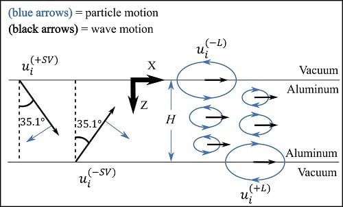
Figure 7.
Conceptual depiction of the partial waves, which are necessary for the S0 Lamb wave problem, overlaid on a plate in vacuum. The angle for the propagation direction of the shear vertical partial waves was calculated using .
Figure 7.
Conceptual depiction of the partial waves, which are necessary for the S0 Lamb wave problem, overlaid on a plate in vacuum. The angle for the propagation direction of the shear vertical partial waves was calculated using .

Figure 8.
Amplitude of the (a) longitudinal (i.e., ) and (b) shear vertical (i.e., ) partial waves after normalizing and averaging the magnitude for various points on the Lamb wave dispersion curves for a 1-mm thick aluminum plate.
Figure 8.
Amplitude of the (a) longitudinal (i.e., ) and (b) shear vertical (i.e., ) partial waves after normalizing and averaging the magnitude for various points on the Lamb wave dispersion curves for a 1-mm thick aluminum plate.

Figure 9.
value which is indicative of the phase difference between the top and bottom partial waves for various points on the Lamb wave dispersion curves for a 1-mm thick aluminum plate. The color axis is constrained to and .
Figure 9.
value which is indicative of the phase difference between the top and bottom partial waves for various points on the Lamb wave dispersion curves for a 1-mm thick aluminum plate. The color axis is constrained to and .

Figure 10.
Depiction of the aluminum slowness curves compared with the slowness curve for air. Slowness curves with solid lines denote real-valued solutions, and dotted lines denote imaginary-valued solutions (figure not to scale).
Figure 10.
Depiction of the aluminum slowness curves compared with the slowness curve for air. Slowness curves with solid lines denote real-valued solutions, and dotted lines denote imaginary-valued solutions (figure not to scale).

Figure 11.
Amplitude of the longitudinal partial waves in the air half-space after normalizing and averaging the magnitude for various points on the Lamb wave dispersion curves for a 1-mm thick aluminum plate. The Lamb wave dispersion curves were calculated assuming traction-free boundary conditions (BC).

Figure 12.
Depiction of the oblique plane wave problem being considered.

Figure 13.
(a) The absolute value, (b) real part, and (c) imaginary part of the amplitude ratios for an incident shear vertical bulk wave at an aluminum–air interface.
Figure 13.
(a) The absolute value, (b) real part, and (c) imaginary part of the amplitude ratios for an incident shear vertical bulk wave at an aluminum–air interface.


Table 1.
Material properties used for the calculations shown in this paper.
| Aluminum [4] | Tungsten [4] | Air [10] | |
|---|---|---|---|
| , kg/m3 | 2700 | 19,250 | 1.2 |
| , GPa | 56.98 | 199.4 | - |
| , GPa | 25.95 | 158.6 | - |
| , m/s | 6350 | 5180 | 343 |
| , m/s | 3100 | 2870 | - |
Table 2.
Eigenvalues and normalized eigenvectors from the Christoffel equation for aluminum at rad/s and rad/m.
Table 2.
Eigenvalues and normalized eigenvectors from the Christoffel equation for aluminum at rad/s and rad/m.
| Partial Waves | , rad/m | |||
|---|---|---|---|---|
| 982.6 | −0.747 | 0 | 0.665 | |
| −982.6 | 0.747 | 0 | 0.665 | |
| 400.0 | −0.341 | 0 | 0.940 | |
| −400.0 | 0.341 | 0 | 0.940 | |
| 400.0 | 0 | 1 | 0 | |
| ) | −400.0 | 0 | −1 | 0 |
Table 3.
Eigenvalues and normalized eigenvectors from the Christoffel equation for tungsten at rad/s and rad/m.
Table 3.
Eigenvalues and normalized eigenvectors from the Christoffel equation for tungsten at rad/s and rad/m.
| Partial Waves | , rad/m | |||
|---|---|---|---|---|
| 997.6 | −0.762 | 0 | 0.648 | |
| −997.6 | 0.762 | 0 | 0.648 | |
| 374.5 | −0.304 | 0 | 0.953 | |
| −374.5 | 0.304 | 0 | 0.953 | |
| 374.5 | 0 | 1 | 0 | |
| ) | −374.5 | 0 | −1 | 0 |
Table 4.
Eigenvalues and normalized eigenvectors from the Christoffel equation for aluminum at rad/s and rad/m.
Table 4.
Eigenvalues and normalized eigenvectors from the Christoffel equation for aluminum at rad/s and rad/m.
| Partial Waves | , rad/m | |||
|---|---|---|---|---|
| 1058.1 | −0.742 | 0 | 0.671 | |
| −1059.1 | 0.742 | 0 | 0.671 | |
| 562.5 | −0.433 | 0 | 0.902 | |
| −562.5 | 0.433 | 0 | 0.902 | |
| 562.5 | 0 | 1 | 0 | |
| ) | −562.5 | 0 | −1 | 0 |
Table 5.
Eigenvalues and normalized eigenvectors from the Christoffel equation for aluminum at rad/s and rad/m.
Table 5.
Eigenvalues and normalized eigenvectors from the Christoffel equation for aluminum at rad/s and rad/m.
| Partial Waves | , rad/m | |||
|---|---|---|---|---|
| 1612.4 | −0.723 | 0 | 0.691 | |
| −1612.4 | 0.723 | 0 | 0.691 | |
| 1339.5 | −0.621 | 0 | 0.784 | |
| −1339.5 | 0.621 | 0 | 0.784 | |
| 1339.5 | 0 | 1 | 0 | |
| ) | −1339.5 | 0 | −1 | 0 |
Table 6.
Method for assigning partial waves to the top or bottom of the plate using the coordinate system shown in Figure 6 and assuming .
Table 6.
Method for assigning partial waves to the top or bottom of the plate using the coordinate system shown in Figure 6 and assuming .
| Top of Plate | Bottom of Plate | |
|---|---|---|
| Real-valued (bulk waves) | and | and |
| Imaginary-valued (surface waves) | and | and |
Table 7.
Eigenvalues and normalized eigenvectors from the Christoffel equation for aluminum at rad/s and rad/m.
Table 7.
Eigenvalues and normalized eigenvectors from the Christoffel equation for aluminum at rad/s and rad/m.
| Partial Waves | , rad/m | |||
|---|---|---|---|---|
| 312.93 | −0.884 | 0 | 0.468 | |
| −312.93 | 0.884 | 0 | 0.468 | |
| 841.13 | −0.818 | 0 | 0.575 | |
| −841.13 | 0.818 | 0 | 0.575 | |
| 841.13 | 0 | 1 | 0 | |
| ) | −841.13 | 0 | −1 | 0 |
© 2018 by the authors. Licensee MDPI, Basel, Switzerland. This article is an open access article distributed under the terms and conditions of the Creative Commons Attribution (CC BY) license (http://creativecommons.org/licenses/by/4.0/).
Share and Cite
MDPI and ACS Style
Hakoda, C.; Lissenden, C.J. Using the Partial Wave Method for Wave Structure Calculation and the Conceptual Interpretation of Elastodynamic Guided Waves. Appl. Sci. 2018, 8, 966. https://doi.org/10.3390/app8060966
AMA Style
Hakoda C, Lissenden CJ. Using the Partial Wave Method for Wave Structure Calculation and the Conceptual Interpretation of Elastodynamic Guided Waves. Applied Sciences. 2018; 8(6):966. https://doi.org/10.3390/app8060966
Chicago/Turabian StyleHakoda, Christopher, and Cliff J. Lissenden. 2018. "Using the Partial Wave Method for Wave Structure Calculation and the Conceptual Interpretation of Elastodynamic Guided Waves" Applied Sciences 8, no. 6: 966. https://doi.org/10.3390/app8060966
Note that from the first issue of 2016, this journal uses article numbers instead of page numbers. See further details here.