Calculation of Guided Wave Dispersion Characteristics Using a Three-Transducer Measurement System

Featured Application

Rapid generation of dispersion curves for guided wave applications when knowledge of the material properties and thickness of the structure to be inspected are unknown.

Abstract

Guided ultrasonic waves are of significant interest in the health monitoring of thin structures, and dispersion curves are important tools in the deployment of any guided wave application. Most methods of determining dispersion curves require accurate knowledge of the material properties and thickness of the structure to be inspected, or extensive experimental tests. This paper presents an experimental technique that allows rapid generation of dispersion curves for guided wave applications when knowledge of the material properties and thickness of the structure to be inspected are unknown. The technique uses a single source and measurements at two points, making it experimentally simple. A formulation is presented that allows calculation of phase and group velocities if the wavepacket propagation time and relative phase shift can be measured. The methodology for determining the wavepacket propagation time and relative phase shift from the acquired signals is described. The technique is validated using synthesized signals, finite element model-generated signals and experimental signals from a 3 mm-thick aluminium plate. Accuracies to within 1% are achieved in the experimental measurements.

1. Introduction

Guided waves have been extensively investigated in the recent years as a nondestructive testing (NDT) technique because of their advantages compared to ultrasonic testing (UT) inspection. The key benefit of this technology is the ability to interrogate the entire thickness of thin-walled structures over large areas from a single location.

During guided wave propagation, waves experience dispersion that distorts the wave shape as the wave propagates, due to a dependence of velocity on frequency [1,2]. Dispersion curves show the relation of phase and group velocities against frequency, for a particular geometry and material. Determination of dispersion curves is important for any guided wave application; accurate dispersion curves enable wave modes of received wavepackets to be distinguished, specific wave modes to be cancelled to clean the acquired signal, the propagation of wave modes in a particular direction using phased arrays [3] and the spatial location of damage in the structure to be determined based on time-of-flight measurements [4]. Guided waves are being used in commercial products, for instance to detect wall thickness losses due to corrosion for pipeline inspection in the oil and gas industry. These commercial products generate a unique wave mode which propagates along the structure avoiding the creation of multimodal excitations, as this would increase the complexity of the analysis of the signals [5,6]. Problems with the application of guided waves occur when the material properties or thickness of the structure to be inspected are unknown due to imprecise records, commercial confidentiality or manufacturing and maintenance uncertainty. This is a particular problem when evaluating composite structures, like wind turbine blades, where elastic constants are not often available. To inspect this kind of structure in an industrial environment, it becomes impracticable as currently there are no means of generating the dispersion curves for such situations. Therefore, there is a need to be able to calculate in situ the phase and group velocities at frequencies of interest in a quick and reliable way without requiring prior knowledge of material properties or thickness.

There has been much work published on the determination of dispersion curves describing many analytical, numerical and experimental methods. For relatively simple structures like plates or pipes, dispersion curves can be predicted using the commercially available software Disperse^®, which uses the global matrix method [7]. Other methods, such as the transfer matrix method [8,9] or pseudospectral collocation method [10], have been utilized to determine dispersion curves. Finite element (FE) [11] and semi-analytical finite element [12,13] methods have been also used. All these numerical and analytical methods require knowledge of material properties and thickness of the structure to determine the dispersion curves.

Experimental methods do not suffer this limitation, since guided wave data is directly acquired from the inspected structure. The most widely used experimental technique to measure dispersion curves is the 2D fast Fourier transform (FFT) [14]. This signal processing technique requires the acquisition of many signals along the wave propagation direction in order to carry out a double FFT in time and space. The result is a wavenumber–frequency matrix, which can be rearranged to give the phase velocity dispersion map. The acquisition of the signals from all required locations is manually prohibitive; therefore, a laser scanning vibrometer (LSV) is commonly used to automatically obtain the signals from preselected points. This device is highly sensitive and bulky, being restricted to controlled areas like laboratories [15] and difficult to use in situ.

Other experimental techniques have been proposed recently. Harb and Yuan [16,17] presented a noncontact technique using an air-coupled transducer (ACT) to generate the wave mode on the plate and an LSV to acquire the propagating mode. The technique requires precise control of the incidence angle of the ultrasonic pressure from the ACT upon the surface. By relating the frequency to the incidence angle at which the wave amplitude is maximized, it is possible to calculate the phase velocity using Snell’s law. However, the technique has limited applicability outside of the laboratory. In works by Mažeika et al. [18,19], a zero-crossing technique is used to calculate the phase velocity based on the measurement of the position of constant phase points of the pulse corresponding to zero amplitude as a function of time. A similar approach is taken in the phase velocity method in [20], tracking the peaks of the pulse rather than the zero crossings. To produce convincing results, both techniques require the acquisition of a large number of signals at different distances, making these techniques time-consuming. For the sake of reducing time and sampling points in space, Adams et al. [21] presented a method using an array probe from which a time–space matrix can be created. A 2D filter is applied to the matrix to extract the phase velocities. The technique was demonstrated to be valid in simulation using FE analysis. However, for realistic probe sizes, the technique has limited experimental applications. In [22], sparse wavenumber analysis was used to experimentally recover the dispersion curves from an aluminum plate; however, seventeen sensors were needed to deploy the technique. An alternative approach to getting dispersion curves from experimental signals is to use time–frequency representations [23], where group velocity can be directly determined. However, the calculation of phase velocity involves the integration of group velocity requiring precise values of ω and k at the lower limit, which are not easy to obtain experimentally. For medical purposes, two techniques, SVD and LRT, were evaluated for extracting the dispersion curves of cortical bones in [24]. Both techniques require a large number of receivers and transmitters.

Experimental calculation of bulk wave velocities in dispersive materials has been studied [25]. Sachse and Pao used the method of phase spectral analysis, where the phase delay is calculated using the real and imaginary parts of the Fourier transform of the pulse, and then obtaining the group delay through the differentiation of the phase characteristics of the pulse with respect to frequency. Pialucha et al. presented the amplitude spectrum technique overcoming the requirement of the phase spectrum technique for the separation of successive pulses in the time domain for bulk waves [26]. However, the phase spectral technique provided better results when pulses can be separated.

In this paper, an experimental technique for straightforward calculations of phase and group velocities of guided waves at frequencies of interest is presented. The technique requires just the acquisition of two signals spaced a few cm using conventional transducers, enabling its application on in-service structures located in poorly controlled environments. There is no requirement for prior knowledge of the material properties or thickness of the inspected structure. In Section 2, the formulation on which the experimental technique relies is presented. Section 3 describes in detail the methodology to extract the group delay and phase shift from experimental signals. Successive sections present validation tests using synthesized signals and simulated signals from FE analysis. Finally, experimental signals from a 3 mm-thick aluminium plate are used to validate the technique as a solution to the problem presented in the introduction.

2. Theoretical Basis

Assuming that the propagating pulse is sufficiently narrow-band that dispersion does not significantly distort the wavepacket over the propagation distance, the signal can be approximated as [27],

$$\psi \left(x,t\right)=G\left(t-\frac{x}{v_g}\right)e^{i\left(kx-\omega t\right)},$$

(1)

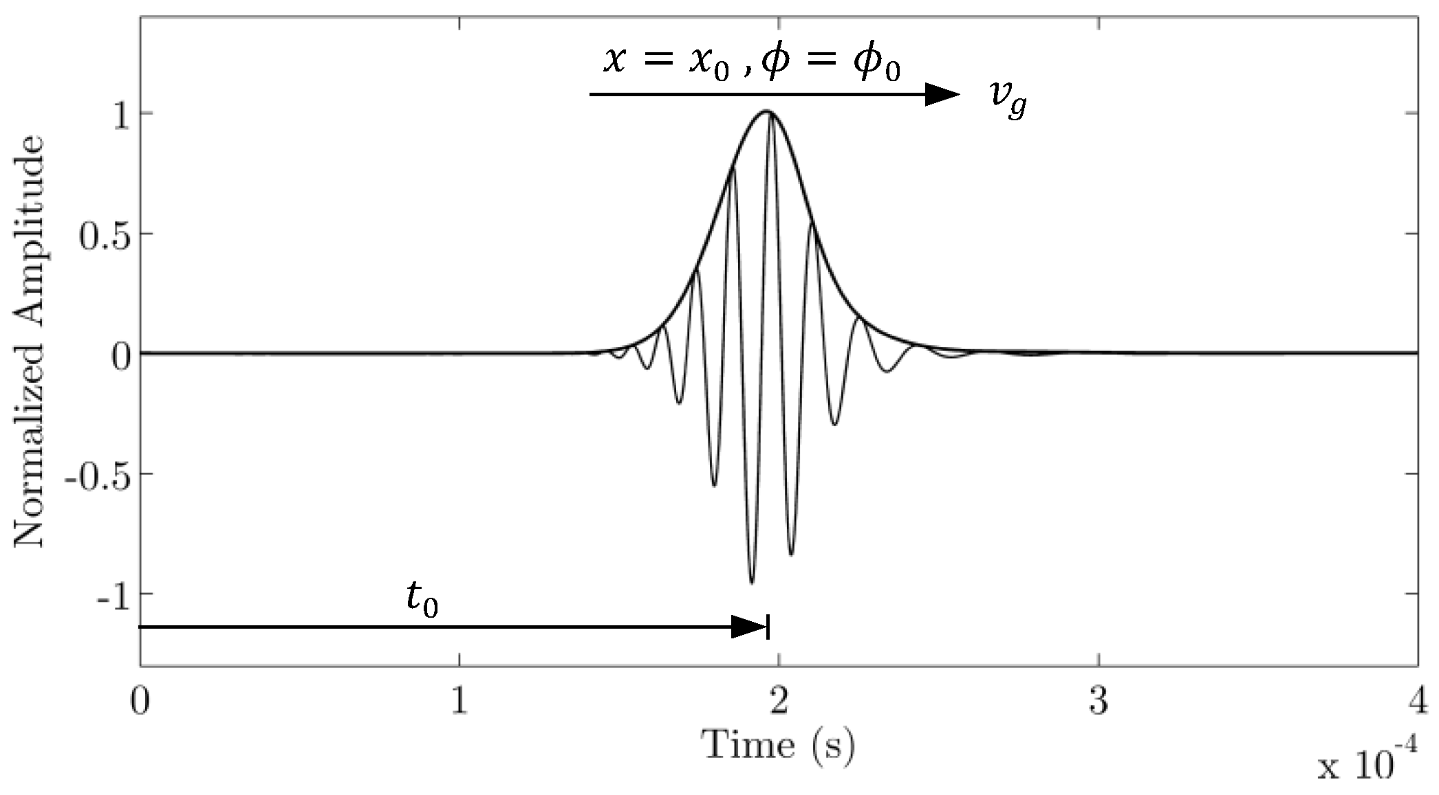
where $x$ is propagation distance, $t$ is time, $\omega =2\pi f$ is the angular frequency of the harmonic wave at frequency $f$ and $k=2\pi /\lambda$ is the wavenumber. $G\left(t\right)$ is a function defining the temporal pulse shape. $G\left(t\right)$ is defined such that the pulse has a peak at $t=0$. $v_g$ is the group velocity at which the packet propagates, and so if the trajectory of the wavepacket peak is defined as the point whereby $G\left(t_0-x_0/v_g\right)=G\left(0\right)$, then

$$v_g=\frac{x_0}{t_0}.$$

(2)

The wavepacket is shown schematically in Figure 1. The harmonic part of the signal has a phase of

$$\varphi =kx-\omega t,$$

(3)

and propagates at the phase velocity [6,27].

$$v_p=\frac{\omega }{k}$$

(4)

The phase of the harmonic signal at the centre of the wavepacket $x_0,t_0$ is

$${\varphi }_0=k{x}_0-\omega t_0.$$

(5)

Rearranging and substituting for $v_p$ and $v_g$ gives

$${\varphi }_0=k{t}_0\left(\frac{x_0}{t_0}-\frac{\omega }{k}\right),$$

(6)

$${\varphi }_0=k{t}_0\left(v_g-v_p\right).$$

(7)

For nondispersive waves, $v_p=v_g$ and Equation (7) gives the expected result that the phase at the wavepacket center is ${\varphi }_0=0$ for all propagation times. Where the system is dispersive there is a finite phase difference between the harmonic part of the signal and the wavepacket, ${\varphi }_0$, which increases linearly with propagation time and is positive if $v_g>v_p$, negative if $v_g<v_p$. Assuming that this phase difference can be measured experimentally, Equations (4) and (5) further yield two useful equations for evaluating the phase velocity:

$$v_p=\frac{x_0-\frac{{\varphi }_0}{k}}{t_0},$$

(8)

$$v_p=\frac{x_0}{t_0+\frac{{\varphi }_0}{\omega }}.$$

(9)

In Figure 2, an illustrative example of a S₀-mode wavepacket at 150 kHz is shown. The solid line is the S₀ mode after 1.2-m propagation including the dispersion. The dashed line represents the S₀ mode after the propagation without dispersion, namely, the wavepacket was calculated using the same phase velocity for all frequencies. In this example, the phase shift is negative (–1.26 radians), which means the phase velocity is higher than the group velocity. Using (9), the calculation of the phase velocity would be 1.2 m divided by the sum of 223 µs, which is the time of the wavepacket to travel 1.2 m at group velocity, plus –1.34 µs which is the time that the signal at an angular frequency, $\omega =2\pi ·150000$, takes to cover –1.26 radians. Group velocity and phase velocity are calculated using (2) and (9), respectively: $v_g=5381m{s}^{-1}$ and $v_p=5414m{s}^{-1}$.

3. Methodology

In this section, the methodology for determining the phase shift and hence the phase velocity is presented. This general methodology is complemented by a description of a specific experiment setup described in Section 6.1. The technique is based on the analysis of two signals acquired at different distances in the direction of wave propagation. One of them will be treated as the baseline and the other signal will be modified in time and phase in order to match with the baseline. The methodology is composed of different signal processing techniques which are presented in a block diagram in Figure 3.

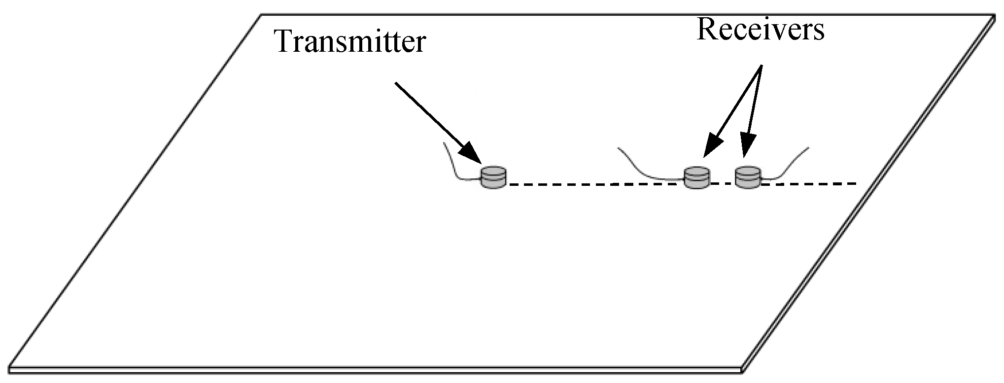
The experimental setup is composed of one transmitter and two receivers along the propagation direction of the wave to be measured, as shown in Figure 4. For isotropic systems the wave velocity is independent of direction. The technique analyses the effect of propagation between the first receiver and the second receiver. Spacing between receivers of a few centimeters is selected in order to avoid large phase shifts and waveform deformations due to dispersion.

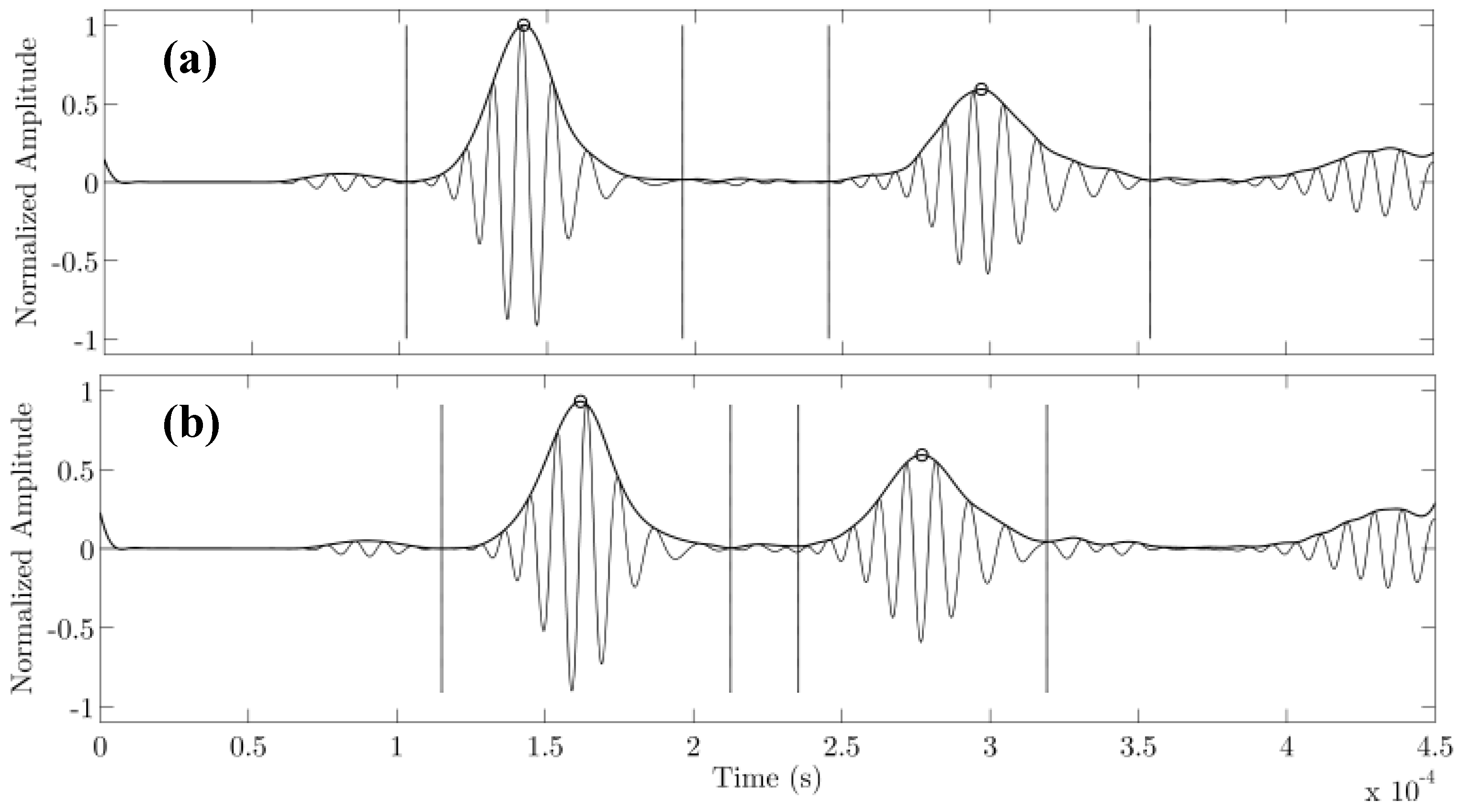
The first step in analyzing the data is the isolation of the desired wavepacket by removing the rest of the signal. The boundaries of each wavepacket are determined by studying the slope of its envelope. The boundaries are set at the closest zero slopes before and after each peak, see example of real signals in Figure 5. Once the region containing the wavepacket is identified, the remainder of the signal is discarded. Both signals are truncated with the same boundaries in order to maintain the time difference between the wavepackets, $w_1$ and $w_2$. The boundaries used are the left limit of the signal of the closest receiver to the transmitter and the second limit of the signal of the further receiver, as can be seen in Figure 6. Afterwards, the Hilbert Transform (H(…)) [28] is applied to both wavepackets and the magnitude extracted in order to determine the envelope of each wavepacket:

$$e_1\left(t\right)=\left|H\left(w_1\left(t\right)\right)\right|,$$

(10)

$$e_2\left(t\right)=\left|H\left(w_2\left(t\right)\right)\right|.$$

(11)

These two envelopes are then cross-correlated to determine the time delay between them:

$$\Delta t=\underset{\tau }{argmax}\left(\left(e_1\star e_2\right)\left(\tau \right)\right),$$

(12)

where $\tau$ is the applied time delay and $\Delta t$ the value that maximizes the correlation. Once this time delay is known, the phase delay to the harmonic part of $w_2\left(t\right)$ that maximizes the cross-correlation between the delayed phase-shifted wavepacket $w_2^{\ast }\left(t-\Delta t\right)$ and $w_1\left(t\right)$ is calculated. This process consists of the modification in phase of the signal from the furthest receiver by a phase angle, $\varphi$, and finding the phase shift that maximizes the cross correlation. The phase shift, $\varphi$, is applied to $w_2^{\ast }$; then, the cross correlation between $w_1$ and $w_2^{\ast }$ is calculated. The optimum phase shift is the phase angle when the correlation coefficient with time delay, $\Delta t$, is highest.

$${\varphi }_{opt}=\underset{\varphi }{argmax}\left(\left(w_1\star w_2^{\ast }\right)\left(\Delta t\right)\left(\varphi \right)\right)$$

(13)

This methodology enables the calculation of the lag time and phase shift between the two signals acquired at different distances. By knowing these three variables (distance, time and phase) and also the excitation frequency, (2) and (9) can be used to determine the group and phase velocity, respectively.

The proposed methodology in this paper is based on the acquisition of two signals spaced a few centimeters apart, since for such short distances the distortion for any wave mode is relatively small, enabling a straightforward determination of the phase shift.

4. Synthetic Signal Analysis

The first validation was carried out using synthesized signals. The signal synthesis is based on the adjustment in frequency and wavenumber of the input signal in the frequency domain. Knowing the waveform at one point, in this case the input signal at the transmitting point, and the dispersion characteristics of each wave mode, the wave modes can be reconstructed in the time domain at any distance [29]. If $u\left(x,t\right)$ is the reconstructed wave mode at a distance $x$ from the transmitting point, $t$ is the time, $F\left(\omega \right)$ is the Fourier transform of the input signal and $k\left(\omega \right)$ is the wavenumber as a function of the angular frequency, then

$$u\left(x,t\right)={\int }_{-\infty }^{\infty }F\left(\omega \right)e^{i\left(k\left(\omega \right)x-\omega t\right)}d\omega$$

(14)

The relation between wavenumber and angular frequency is extracted directly from the dispersion curves provided by Disperse^® and introduced in the integral.

As an initial test of the signal processing method, developed signals are synthesized that are highly pure, without noise and overlapping between modes. The higher the sampling frequency is set, the better accuracy the technique provides. The sampling frequency was set at 10 MHz, since it has been observed that it provides a good balance between computational time and accuracy.

A set of signals for symmetric (S₀), antisymmetric (A₀) and shear horizontal (SH₀) wave modes were created by evaluating equation (14) in MATLAB for two propagation distances, 30 cm and 35 cm: the analysed propagated distance ($\Delta d$) in this case is 5 cm. The analysed frequencies are from 60 to 370 kHz with steps of 10 kHz.

The results after applying the signal processing algorithm described in Section 3 to the synthesized signals are presented in Figure 7. The results (black circles) accurately reconstruct the theoretical values from Disperse^® (grey lines). In Figure 8, the extracted phase shift has been represented against the frequency for the three fundamental modes. For the S₀ mode, the phase values have negative values decaying from –2 degrees at 60 kHz to –52 degrees at 370 kHz. For the A₀ mode, conversely, the phase is positive, increasing along the frequency, since the phase velocity is lower than the group velocity; from 377 degrees at 60 kHz to 673 degrees at 370 kHz. In this case, the phase values are much higher than the S₀ and SH₀ ones, because the A₀ mode is highly dispersive at these frequencies. For the SH₀ mode, the extracted phase values are 0 degrees at 60 kHz and 1 degree at 370 kHz. The SH₀ is a nondispersive mode so the phase value remains at near 0 degrees.

The sampling frequency is an important factor, since it determines the degree of resolution of the group velocity. As these examples are performed for short propagation distances, the time that the wave modes take to cover that distance is small. Thus, low sampling frequencies are not able to determine the group velocity accurately. Faster modes require higher sampling frequencies to get the same resolution as slower modes. In this case of 5 cm spacing, the propagation time for the S₀ mode at 200 kHz is 9.3 µs; a sampling frequency of 1 MHz will have a time resolution of 1 µs which yields a velocity resolution for this particular example of 556 m/s; with a sampling frequency of 10 MHz, the velocity resolution will be 58.4 m/s; and with a sampling frequency of 100 MHz, the velocity resolution will be 5.8 m/s. This resolution issue can be observed in Figure 7; at lower velocities the curves are smoother, and at higher velocities (S₀ mode) the curves have poorer velocity resolution.

5. Finite Element Analysis

A three-dimensional FE analysis was performed in Abaqus to simulate signals. While the previous analysis required the input of the dispersion curves to create the propagated signals, this FE analysis does not require prior knowledge of the dispersion characteristics.

FE models were created simulating guided wave propagation at five different frequencies in an aluminium plate (1000 × 1000 × 3 mm). The transmitter and receivers were modelled as ideal point transducers. The transmitting point was placed at the centre of the plate, where the coordinate system was established. A force was applied in the x-direction to simulate a shear transducer. This generated S₀ and A₀ modes along the x-axis and the SH₀ mode along the y-axis. The input signal was a 5-cycle sine with a Hanning window at central frequencies of 60, 80, 100, 120 and 140 kHz. Multiple receiver points were located on the positive x-axis and positive y-axis from the centre of the plate to the edge every 1 cm, resulting in 50 receivers at each axis. The time and spatial discretization for the finite element model was established at 10^-2 µs and 1 mm, respectively, in order to ensure convergence and to obey the Nyquist sample-rate criterion. The mesh was formed by C3D8 elements.

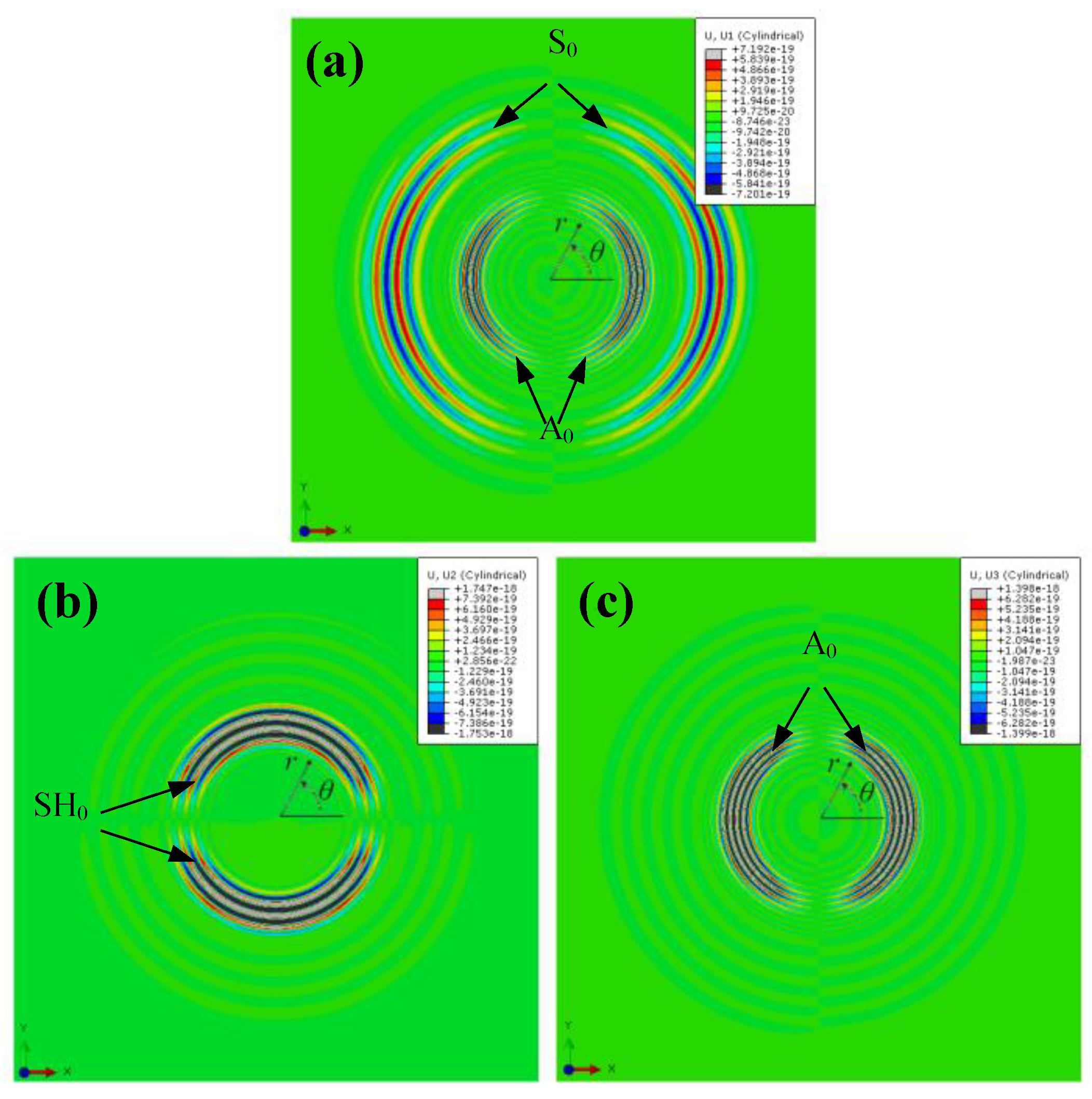
The FE analysis software provides the results decoupled for each axis direction, so it is straightforward to evaluate each wave mode separately. In Figure 9, the results have been computed in cylindrical coordinates to show clearly the three wave modes of propagation at each axis. In Figure 9a, showing radial displacement, S₀ and A₀ modes are depicted, S₀ being the faster mode. In Figure 9b showing tangential displacement, the SH₀ mode propagates along the y-axis, and in Figure 9c, showing out-of-plane displacement, the A₀ mode is clearly present.

Since the plate is relatively small, overlaps between wave modes and echoes from edges are produced, as can be seen in Figure 10. This is a particular problem at lower frequencies (60 and 80 kHz) due to the length of the pulses. Therefore, an additional optimisation step has been added to minimize the error introduced by the overlapping. The FE model has 50 receiver points, every 1 cm along the axis so the five least-overlapped signals are selected for analysis. The selection is performed by analyzing the amplitude at the beginning and end of the envelope of the wavepacket of interest; the signals with the lowest amplitude at those regions are selected. Then, the signal processing described in Section 3 is applied for all the pair combinations between the five selected receivers. Once the phase and group velocities are calculated for each combination, the velocities are averaged to give the final velocity estimates. Any outliers that are introduced during selection of the five signals are eliminated. As shown in Figure 11, the phase velocity matches very well with the theoretical values from Disperse^®. In the group velocity graph, the results correlate well with the theoretical velocities, having a noticeable variation in the S₀ value at 60 kHz. This variation occurs at 60 kHz due to the overlap between the S₀ mode and the A₀ mode, which is more pronounced for the longer pulses at this frequency. This error does not appear for the A₀ mode because the signals used for the analysis were out-of-plane displacements, where the S₀ mode is practically imperceptible. Note that the results improve as the frequency increases, since the wavelength decreases and mode separation increases. Overlapping of pulses is an issue for this technique, as it changes the phase and waveform of the analyzed mode, highly distorting the results and impeding its application.

The results for the phase velocity are better than for the group velocity, more notably when overlapping occurs. This is because of the phase-shift term in the denominator in (9). This contribution in the phase velocity equation minimizes the erroneous calculated value of the propagation time and also provides more resolution on the calculation of the phase velocity, removing the stepped shape seen in the group velocity.

6. Experimental Demonstration

6.1. Test Setup

The specimen is a 4 m by 2 m aluminium plate of 3 mm thickness. Two piezoelectric transducers were used, one transmitter and one receiver. The transmitter was fixed at the centre of the plate using a tool that provides force over the transducer; and the receiver was manually attached at various distances from the transmitter. For the evaluation of the S₀ mode, the receiver was placed at 45, 50 and 55 cm from the transmitter. For the case of the A₀ and SH₀ modes, the receiver was set at 25, 30 and 35 cm from the transmitter. Those distances were selected to minimize the wavepacket distortion due to overlaps.

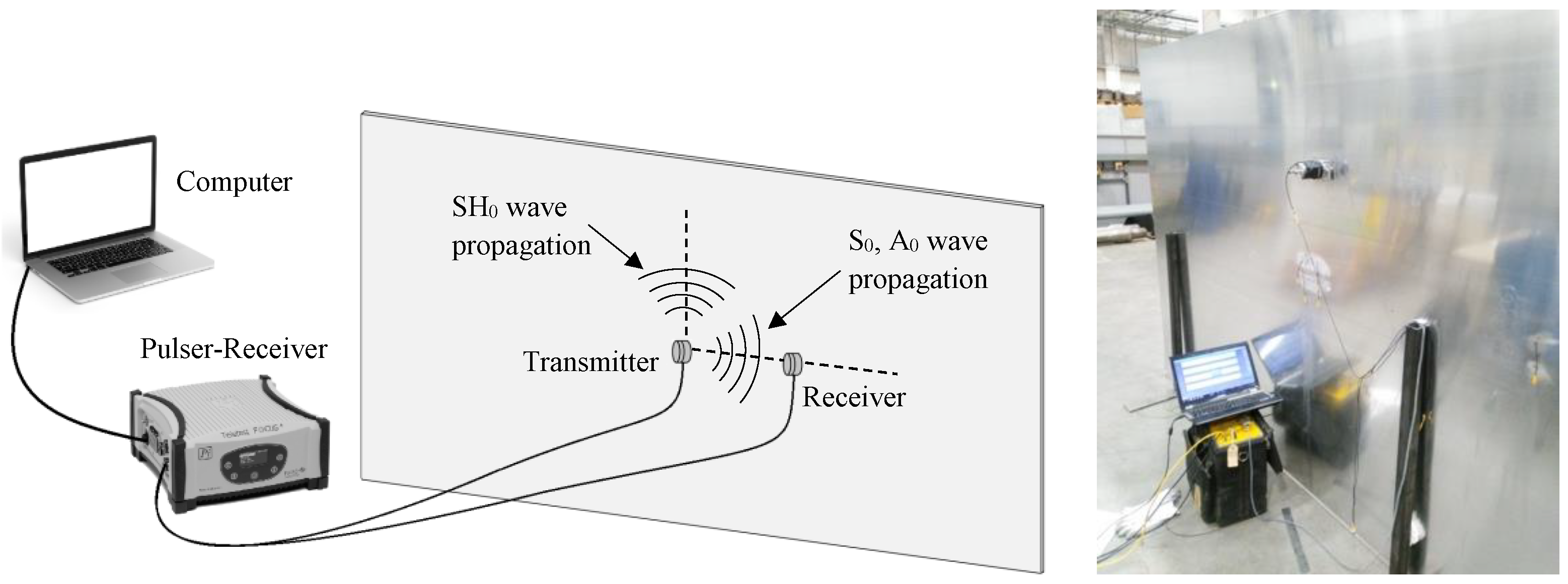
A pulser-receiver (Teletest^® unit) was used to excite the transducer and acquire the signals. Two independent channels were used for the excitation and acquisition. A PC with the Teletest^® software was used to control the pulser-receiver and configure the experimental parameters. Input signals of five-cycle Hanning-windowed bursts with centre frequencies from 40 kHz to 140 kHz in steps of 5 kHz were used to excite the transmitter. This frequency range was chosen since it is the operating frequency range of the transducers used in the experiment. Signals were recorded with a 1 MHz sampling frequency; 32 averages were taken, and the record length of the signals was 1 ms. The experimental setup is presented in Figure 12.

Two types of piezoelectric transducers (PI Ceramic GmbH) were used in the experiment, a shear piezoelectric element (d₁₅ type) and a compressional piezoelectric element (d₃₃ type), both with an active contact area of 13 mm by 3 mm. Figure 13 shows the direction of poling and corresponding shear deformation for the shear transducer. The shear transducer was used to evaluate the S₀ and SH₀ wave modes, and the A₀ wave mode was analyzed using the compressional transducer, which mainly produces an out-of-plane vibration. Using the shear transducer, S₀ waves are generated in the direction of the poling axis, and SH₀ in the perpendicular axis. A small amount of A₀ is also generated on the poling axis. In the case of the compressional transducer, S₀ and A₀ are created omnidirectionally. The averaged amplitudes of the S₀ and SH₀ modes using the shear transducer at the propagation distances specified above are 13 mV and 33 mV, respectively; and the amplitude of the A₀ mode is 63 mV using the compressional transducer.

Experimental signals were acquired at a sampling frequency of 1 MHz providing a poor time resolution for the wave velocities of interest. Therefore, the sampling rate of the signals was increased by a factor of 10 using cubic spline interpolation to give a time accuracy of 0.1 µm (10 MHz). The interpolation is a necessary step when the propagation distance is a few cm, as the propagation time of the faster modes, such as S₀, is of the same order of magnitude as the original sampling period. By reducing the sampling period by means of interpolation, the accuracy of the group velocity is increased. However, a small error is introduced in the signal due to the interpolation. Overall, the improvements gained for the velocity calculation are more significant than the errors introduced in the signals. The signal-to-noise ratios of the S₀, A₀ and SH₀ signals were around 30 dB, 37 dB and 35 dB, respectively.

6.2. Experimental Results

The results presented in Figure 14 and Figure 15 have been extracted from signals at two different spacings: 5 cm and 10 cm. The velocities extracted from the experimental signals correlate quite well with the theoretical velocities. However, there are slight variations around the theoretical velocities. These variations can be caused by a number of factors, such as the aforementioned interpolation and overlapping, but also by the manipulation of the transducers, which in this case were handled manually. Small variations in the correct spacing distance between transducers lead to errors in the calculation of the velocities. The velocity–distance relationship is linear so the relative error in the calculated velocity due to misplacement is the same as the relative distance error. An error of 1 mm in an intended 5 cm spacing distance will cause a 2% error in the velocity or an error of 110 ms^-1 in the S₀ mode (≈ 5400 m/s), for example. On the other hand, with a 1 mm error transducer placement for a 10 cm spacing, the error will be of 1% of the velocity. Therefore, large errors can occur where small propagation distances are used. A₀ and SH₀ exhibit less absolute error variation than S₀ due to their slower velocities, the generated errors being proportional to the velocity.

In this paper, two propagation distances have been chosen: 5 and 10 cm. From the S₀ mode in Figure 15, it can be seen that the calculated velocities at 10 cm are more accurate, and the variance is also smaller. This is for two reasons: the first is the reduction in the error caused by an incorrect transducer placement, and the second is the implicit increase of the propagation time, which reduces the error in determining that time. Other factors that can introduce errors in the velocity calculation are the variations of the boundary conditions of the transducer, such as the applied pressure over the transducer at each receiving location, as well as the difference of transfer function of each transducer. This problem was overcome utilizing the same transducer to acquire the signals at all locations. Similarly, a change in temperature between measurements will cause velocity changes leading to erroneous values. This can be avoided by acquiring results in quick succession to minimize the impact of the temperature in the results. Using three transducers, one transmitter and two receivers would avoid the issues relating to moving the transducers.

7. Conclusions

This paper has presented a new methodology for creating dispersion curves based on measuring the phase difference and time lag between two pulses acquired at different distances. Firstly, the theoretical basis of the method has been presented where the phase velocity has been related to the phase at the pulse centre for systems of limited dispersion; then, a signal processing methodology to extract the phase shift and time lag between two signals and subsequently calculate the phase and group velocities has been outlined. Three different tests were performed to validate the formulation and methodology; using synthesized signals, signals from an FE model and experimental signals. In the three cases the performance achieved agrees well with the theoretical values.

There are some limitations to the proposed method for the extraction of the phase shift to calculate the dispersion curves. Highly dispersive modes, like high-order modes, are more challenging to evaluate; to mitigate this issue, much shorter spacing distances between transducers should be established to minimize the mode-shape distortion. Overlapping between wavepackets limits the method’s applicability, since it distorts the apparent phase of the mode being analyzed. Hence, relatively large samples are required to avoid overlapping between wavepackets and edge echoes. The size of the sample can be smaller at higher frequencies. The velocity–frequency spectrum that can be evaluated using this method will be determined by the excitation mechanism used to generate the guided waves in the solid media. With appropriate experimental design, errors of less than 1% are obtained.

For future work, the proposed technique will be applied to more complex structures, such as composite plates where the elastic constants are not easy to obtain. In this case, by studying the phase and group velocities as a function of propagation direction, the full angular dependency of the dispersion curves will be obtained.

References

- Rose, J.L. Ultrasonic Waves in Solid Media; Cambridge University Press: Cambridge, UK, 1999. [Google Scholar]
- Wilcox, P.; Lowe, M.; Cawley, P. The effect of dispersion on long-range inspection using ultrasonic guided waves. NDT E Int. 2001, 34, 1–9. [Google Scholar] [CrossRef]
- Wang, W.; Zhang, H.; Lynch, J.P.; Cesnik, C.E.; Li, H. Experimental and numerical validation of guided wave phased arrays integrated within standard data acquisition systems for structural health monitoring. Struct. Control Health Monit. 2018, 25, e2171. [Google Scholar] [CrossRef]
- Wang, W.; Bao, Y.; Zhou, W.; Li, H. Sparse representation for Lamb-wave-based damage detection using a dictionary algorithm. Ultrasonics 2018, 87, 48–58. [Google Scholar] [CrossRef] [PubMed]
- Cawley, P.; Lowe, M.; Alleyne, D.; Pavlakovic, B.; Wilcox, P. Practical long range guided wave inspection-applications to pipes and rail’. Mater. Eval. 2003, 61, 66–74. [Google Scholar]
- Rose, J.L. Ultrasonic Guided Waves in Solid Media; Cambridge University Press: Cambridge, UK, 2014. [Google Scholar]
- Pavlakovic, B.; Lowe, M.; Alleyne, D.; Cawley, P. Disperse: A general purpose program for creating dispersion curves. In Review of Progress in Quantitative Nondestructive Evaluation; Springer: Boston, MA, USA, 1997; pp. 185–192. [Google Scholar]
- Lowe, M.J. Matrix techniques for modeling ultrasonic waves in multilayered media. IEEE Trans. Ultrason. Ferroelectr. Freq. Control 1995, 42, 525–542. [Google Scholar] [CrossRef]
- Nayfeh, A.H. “The general problem of elastic wave propagation in multilayered anisotropic media. J. Acoust. Soc. Am. 1991, 89, 1521–1531. [Google Scholar] [CrossRef]
- Quintanilla, F.H.; Fan, Z.; Lowe, M.; Craster, R. Dispersion loci of guided waves in viscoelastic composites of general anisotropy. In AIP Conference Proceedings; AIP Publishing: Melville, NY, USA, 2016; Volume 1706, p. 120014. [Google Scholar]
- Yu, X.; Ratassepp, M.; Fan, Z. Damage detection in quasi-isotropic composite bends using ultrasonic feature guided waves. Compos. Sci. Technol. 2017, 141, 120–129. [Google Scholar] [CrossRef]
- Hayashi, T.; Song, W.-J.; Rose, J.L. Guided wave dispersion curves for a bar with an arbitrary cross-section, a rod and rail example. Ultrasonics 2003, 41, 175–183. [Google Scholar] [CrossRef]
- Cong, M.; Wu, X.; Liu, R. Dispersion analysis of guided waves in the finned tube using the semi-analytical finite element method. J. Sound Vib. 2017, 401, 114–126. [Google Scholar] [CrossRef]
- Alleyne, D.; Cawley, P. A two-dimensional Fourier transform method for the measurement of propagating multimode signals. J. Acoust. Soc. Am. 1991, 89, 1159–1168. [Google Scholar] [CrossRef]
- Ostachowicz, W.; Güemes, A. New Trends in Structural Health Monitoring; Springer Science & Business Media: London, UK, 2013; Volume 542. [Google Scholar]
- Harb, M.; Yuan, F. A rapid, fully non-contact, hybrid system for generating Lamb wave dispersion curves. Ultrasonics 2015, 61, 62–70. [Google Scholar] [CrossRef] [PubMed]
- Harb, M.; Yuan, F. Non-contact ultrasonic technique for Lamb wave characterization in composite plates. Ultrasonics 2016, 64, 162–169. [Google Scholar] [CrossRef] [PubMed]
- Mažeika, L.; Draudvilienė, L. Analysis of the zero-crossing technique in relation to measurements of phase velocities of the Lamb waves. Ultragarsas 2010, 65, 7–12. [Google Scholar]
- Draudvilienė, L.; Aider, H.A.; Tumsys, O.; Mažeika, L. The Lamb waves phase velocity dispersion evaluation using an hybrid measurement technique. Compos. Struct. 2018, 184, 1156–1164. [Google Scholar] [CrossRef]
- Moreno, E.; Galarza, N.; Rubio, B.; Otero, J.A. Phase Velocity Method for Guided Wave Measurements in Composite Plates. Phys. Procedia 2015, 63, 54–60. [Google Scholar] [CrossRef]
- Adams, C.; Harput, S.; Cowell, D.; Freear, S. A phase velocity filter for the measurement of Lamb wave dispersion. In Proceedings of the 2016 IEEE International Ultrasonics Symposium (IUS), Tours, France, 18–21 September 2016; pp. 1–4. [Google Scholar]
- Harley, J.B.; Moura, J.M. Sparse recovery of the multimodal and dispersive characteristics of Lamb waves. J. Acoust. Soc. Am. 2013, 133, 2732–2745. [Google Scholar] [CrossRef] [PubMed]
- Latif, R.; Aassif, E.; Maze, G.; Moudden, A.; Faiz, B. Determination of the group and phase velocities from time-frequency representation of Wigner-Ville. NDT E Int. 1999, 32, 415–422. [Google Scholar] [CrossRef]
- Xu, K.; Ta, D.; Cassereau, D.; Hu, B.; Wang, W.; Laugier, P.; Minonzio, J.-G. Multichannel processing for dispersion curves extraction of ultrasonic axial-transmission signals: Comparisons and case studies. J. Acoust. Soc. Am. 2016, 140, 1758–1770. [Google Scholar] [CrossRef] [PubMed]
- Sachse, W.; Pao, Y.-H. On the determination of phase and group velocities of dispersive waves in solids. J. Appl. Phys. 1978, 49, 4320–4327. [Google Scholar] [CrossRef]
- Pialucha, T.; Guyott, C.; Cawley, P. Amplitude spectrum method for the measurement of phase velocity. Ultrasonics 1989, 27, 270–279. [Google Scholar] [CrossRef]
- Graff, K.F. Wave Motion in Elastic Solids; Courier Corporation: Chelmsford, MA, USA, 2012; pp. 62–65. [Google Scholar]
- Michaels, J.E.; Lee, S.J.; Croxford, A.J.; Wilcox, P.D. Chirp excitation of ultrasonic guided waves. Ultrasonics 2013, 53, 265–270. [Google Scholar] [CrossRef] [PubMed]
- Wilcox, P.D. A rapid signal processing technique to remove the effect of dispersion from guided wave signals. IEEE Trans. Ultrason. Ferroelectr. Freq. Control 2003, 50, 419–427. [Google Scholar] [CrossRef] [PubMed]
Figure 1.
Wavepacket arriving at at time with phase propagating at group velocity . is represented as the envelope of the wavepacket.
Figure 2.
S0-mode wavepacket of 5 cycles at 150 kHz after propagating 1.2 m, with dispersion and without dispersion.
Figure 3.
Methodology’s block diagram to extract the optimum phase shift and time delay.
Figure 4.
Schematic of the test setup.
Figure 5.
Wavepacket detection and boundary determination established by the algorithm for two signals acquired at: (a) 30 cm and (b) 35 cm from the transmitter using a d33-type transducer.
Figure 6.
Shortening of the signals to reduce computational time. The same limits are used to truncate each signal in order to maintain the time difference between wavepackets. Signals acquired at: (a) 30 cm and (b) 35 cm from the transmitter.
Figure 7.
Comparison of the phase velocity and group velocity of , and between the results from the synthesized signals (black circles) and theoretical values (grey lines).
Figure 8.
Comparison of the phase shift of S0, A0 and SH0 between the results from the synthesized signals (black circles) and theoretical values (grey lines).
Figure 9.
Images of the finite elementsimulation of the wave propagation in polar-coordinate instantaneous displacement is shown 76 µs after excitation. (a) Radial displacement, (b) tangential displacement and (c) out-of-plane displacement. Scale bars in meters.
Figure 10.
Signal acquired at 33 cm from excitation point at 60 kHz.
Figure 11.
Comparison of the phase velocity and group velocity of S0, A0 and SH0 between the results from the synthesized signals (black circles) and theoretical values (grey lines).
Figure 12.
Experiment setup: Left–diagram of the experiment, Right–photo of the real experiment environment.
Figure 13.
Schematics of the shear transducer. (a) Undeformed, (b) deformed.
Figure 14.
Phase velocity and group velocity created from experimental signals for 5 cm propagation distance (black circles) and theoretical values (grey lines).
Figure 15.
Phase velocity and group velocity created from experimental signals for 10 cm propagation distance (black circles) and theoretical values (grey lines).
© 2018 by the authors. Licensee MDPI, Basel, Switzerland. This article is an open access article distributed under the terms and conditions of the Creative Commons Attribution (CC BY) license (http://creativecommons.org/licenses/by/4.0/).
Share and Cite
MDPI and ACS Style
Hernandez Crespo, B.; Courtney, C.R.P.; Engineer, B. Calculation of Guided Wave Dispersion Characteristics Using a Three-Transducer Measurement System. Appl. Sci. 2018, 8, 1253. https://doi.org/10.3390/app8081253
AMA Style
Hernandez Crespo B, Courtney CRP, Engineer B. Calculation of Guided Wave Dispersion Characteristics Using a Three-Transducer Measurement System. Applied Sciences. 2018; 8(8):1253. https://doi.org/10.3390/app8081253
Chicago/Turabian StyleHernandez Crespo, Borja, Charles R. P. Courtney, and Bhavin Engineer. 2018. "Calculation of Guided Wave Dispersion Characteristics Using a Three-Transducer Measurement System" Applied Sciences 8, no. 8: 1253. https://doi.org/10.3390/app8081253
Note that from the first issue of 2016, this journal uses article numbers instead of page numbers. See further details here.