The Generation Mechanism of the Flow-Induced Noise from a Sail Hull on the Scaled Submarine Model

1
Acoustic science and technology laboratory, Harbin Engineering University, Harbin 150001, China
2
Key laboratory of marine information acquisition and security (Harbin Engineering University), Ministry of Industry and Information, Harbin 150001, China
3
College of underwater acoustic engineering, Harbin Engineering University, Harbin 150001, China
*
Author to whom correspondence should be addressed.
Appl. Sci. 2019, 9(1), 106; https://doi.org/10.3390/app9010106
Submission received: 22 November 2018
/
Revised: 24 December 2018
/
Accepted: 24 December 2018
/
Published: 29 December 2018
(This article belongs to the Special Issue Active and Passive Noise Control)
Abstract
:Featured Application
The results in this research can provide the design orientation for the flow control techniques to suppress the hydrodynamic noise from the sail hull. The results can also lay the foundation for the novel design of the sail hull with a low level of the flow-induced noise.
Abstract
Flow-induced noise from the sail hull, which is induced by the horseshoe vortex, the boundary layer separation and the tail vortex shedding, is a significant problem for the underwater vehicles, while has not been adequately studied. We have performed simulations and experiments to reveal the noise generation mechanism from these flows using the scaled sail hull with part of a submarine body. The large eddy simulation and the wavenumber–frequency spectrum are adopted for simulations. The frequency ranges from 10 Hz to 2000 Hz. The simulation results show that the flow-induced noise with the frequency less than 500 Hz is mainly generated by the horseshoe vortex; the flow-induced noise because of the tail vortex shedding is mainly within the frequency of shedding vortex, which is 595 Hz in the study; the flow-induced noise caused by the boundary layer separation lies in the whole frequency range. Moreover, we have conducted the experiments in a gravity water tunnel, and the experimental results are in good accordance with the simulation results. The results can lay the foundation for the design of flow control devices to suppress and reduce the flow-induced noise from the sail hull.
1. Introduction
With excellent concealment, submarines are one of the most critical naval weapons in the ocean. However, the noise radiated by the submarines during movement is a direct threat to their safety, and noise control of submarines has become a hot issue nowadays. Generally speaking, the noise radiated by a submarine can be divided into three categories: hydrodynamic noise, mechanical vibration noise, and propeller noise. If the submarine runs over a speed of 12 knots, the hydrodynamic noise will be the dominant noise source, compared to the mechanical vibration noise and propeller noise, of which the mechanisms have been sufficiently investigated [1,2,3]; the other two noises have been efficiently controlled [4] by modern technology.
When the fluid flows around the submarine, two kinds of noises will be generated. The turbulent fluctuation pressure in the flow radiates a noise, which is called the flow noise. The elastic shell of the submarine is excited by the turbulent fluctuation pressure, and radiates the flow-induced noise. The hydrodynamic noise is the summation of the flow noise and the flow-induced noise. Since the sound pressure level of the flow noise is much lower than that of the flow-induced noise, the flow noise is usually negligible. In some conditions, the flow-induced noise can be described as the hydrodynamic noise. Recently, some phenomena of the flow-induced noise from underwater elastic structures similar to the submarines have been revealed, and the techniques of the flow control to reduce the hydrodynamic noise have been investigated [5,6]. However, these researches are only concerned in the optimization of the shape, which is probably not suitable for the submarines, because the optimization of the shape will squeeze some space of the submarines and is hardly to be carried out in practical engineering.
As we know, the hydrodynamic noise of the submarines comes from the bow, the sail hull, the stern, and the propeller, which is mentioned earlier. The noise generation mechanism of the submarine is complicated because of its complex structure. The previous studies on the flow-induced noise of the submarines stem from the cylinder for its simple structure [7], and some analytical equations are obtained. However, the bow, the sail hull and the stern of the submarine are not symmetric, and the exact analytic solutions of the flow-induced noise cannot be reached like what Rocha et al. [8] have done. Therefore, the direct experimental observation is also another commonly adopted method [9,10]. After that, with the development of computational capability, the numerical calculation has become a powerful tool to analyze the flow-induced noise from these complicated structures [11,12]. The numerical calculation is usually done by coupling a Reynolds-averaged Navier–Stokes hydrodynamic solver to a hydroacoustic code implementing different resolution forms of the Ffowcs Williams–Hawkings (FW–H) equation [13]. From numerical simulation, we can draw some results of the flow-induced noise from the structures, which is similar to part of the submarines. Qu et al. has studied the characteristics of flow field and hydrodynamic noise of trapezoidal rudder wing under different rudder angles by the simulation, and have found that the sound pressure level spectrum band of the flow noise is full and there is no apparent dominant frequency [14]. Li et al. has proposed the mutual coupling method between the vulcanized rubber layer and the flow around to solve the flow field and the noise field for an axisymmetric body in water, and have found that noise power levels in the peak of the axisymmetric body are lower than those in the other positions [15]. Ozden et al. has numerically calculated the propeller noise from the INSEAN E1619 submarine propeller in open water and have found that noise propagation in the study is a spherical spreading model [16]. Besides, with the fine grids of the model, the flow-induced noise from different flow phenomena can be investigated, and the noise generation mechanism can be analyzed in detail [17]. Furthermore, the characteristics of sub-boundary layer sound generation have been studied by Con et al., who have found that the rectangular steps produce more noise than the triangular steps, which is most likely due to the differences in the turbulent flow environment at the front surfaces of the steps [18]. After the analysis from the numerical calculation, the experimental measurement [10,19] becomes essential to validate the calculated results, which can reveal the properties of the flow-induced noise, because the precision of the numerical calculation is limited by the number of the grids and the defects of the boundary element method [20].
To suppress the hydrodynamic noise from the submarines, we must know the exact noise sources from the excitation of different flow phenomena. One of the sources of the hydrodynamic noise is from the excitation by the horseshoe vortex. Liu et al. have proposed the modified method of a vortex baffle to break the vortex core of the horseshoe vortex [6]. Since the horseshoe vortex is a giant vortex mass, from which the noise is in the low-frequency range, the control of the horseshoe vortex neglects the noise of high-frequency range. Aiming to describe the relationship between hydraulic and acoustic conditions, this research will provide a better understanding of noise source acoustical characteristics and show the influence of geometrical parameters on noise production and emission, just like what Prek has done in a water installation system [21]. Furthermore, the exact understanding of the generation mechanism of the flow-induced noise can help us better separate the needed noise components from other noises with the disturbance of the hydrodynamic noise [22].
Although there are some mature studied reports in the airfoil [14,19], which can be considered as similar to the sail hull and the stern of the submarine, these results can only be references. One difference of the results between the water and the air is the assumption that the feedback of the acoustic field to the flow is small for low Mach number flows [23] in the air. Because the water is the dense medium, of which the acoustic impedance is approximately equal to that of the submarine, the feedback of the acoustic field to the flow cannot be considered as small or neglected. Another difference in the results between the two is the experimental measurement. In the air experimental facilities, the model is placed at the outlet of the wind tunnel and the driven air can be dispersed everywhere. The third difference in the results between the water and the air is that the Reynolds number is lower and no cavitation occurs in the air, compared to that in the water. All these differences can be the obstacles when the results of the air are applied into the water.
In our study, based on the theory of numerical simulation [24], we have proposed the method to calculate the flow-induced noise from the model of the sail hull with part of the submarine body. The flow field is calculated by the Large Eddy Simulation (LES), and the sound sources which are on the right-hand side of the acoustic equations are extracted from the computed flow field. After that, we have introduced the method of the wavenumber–frequency spectrum to calculate the flow-induced noise, to conquer the overestimate effect of the FW-H equation in the near sound field; at the same time, to avoid the problem that the solution is not unique in the characteristic frequency of the boundary element method. In the simulation, we have investigated the generation mechanism of the flow-induced noise from three kinds of the flow phenomena around the sail hull and part of the submarine body, which are the horseshoe vortex, the boundary layer separation, and the tail vortex shedding. We also have analyzed the sound field and the frequency characteristic of the flow-induced noise from these three kinds of flow phenomena. Creating a model of the sail hull with part of the submarine body, we have conducted the experiments in the gravity water tunnel. To avoid the influence of the impact on the hydrophone, we have adopted the reverberation method to measure the sound radiation power in a water tank outside the working section in the gravity water tunnel. The experimental results coincide well with that of the numerical simulation. Therefore, the analysis of the generation mechanism of the flow-induced noise is validated by the experiments.
2. Theory of Numerical Simulation
2.1. LES Method
The flow field of the model is numerically calculated by LES, and turbulent fluctuation pressure is extracted from the simulation. In the theory of LES, turbulent vortices are divided into two parts: large-scale vortex and small-scale vortex. The large-scale vortex provides the major part of the turbulent energy. However, the small-scale vortex only dissipates the turbulent energy. More specifically, a filter function is established in the method, which can filter out the small-scale vortex. The large-scale vortex is introduced into the Navier–Stokes equation (NS) and solved. The sub-grid stress terms are added to the NS equation to show the effect of the small-scale vortex on the flow field. The filtered NS equation is as follows:
where is the term of sub-grid stress, and is also called the filtered stress tensor. The dynamic sub-grid model proposed by Germano is added to make Equation (1) enclosed [25], which can be suitably adapted into the local turbulent structure near the wall.
where is the coefficient of sub-grid eddy viscosity, is the sub-grid scale Reynolds stress, and is the rate of strain tensor, which can be written as:
where is the scale of the filter, and is equivalent to the mix length. The dynamic sub-grid model needs to be continuously adjusted to suit different computational processes. The convection field needs to be filtered many times, and the results are as follows:
where is the resolved stress, and is the tensor.
2.2. Theory of Vibration and Sound Radiation by the Flow-Induced Force
When the fluid flows around the model, the shell will be vibrated under the flow-induced force. Then, the noise will be radiated from the model by the excitation of the flow. In the theory of the vibration and sound radiation from the shell under the flow-induced force, some assumptions need to be held as follows.
(1) The turbulent pressure field is spatially uniform, and is static relative to time. That is, the time–spatial correlation of wall pressure fluctuation only depends on spatial distance and time interval.
(2) The sound radiation from the vibration of the model is under the excitation of turbulent fluctuation pressure, while that from the turbulent fluctuation pressure itself is ignored.
(3) The properties of the model are isotropic and obey the theory of the elasticity.
If denotes turbulent fluctuation pressure, which excites the shell of the model, can be decomposed by the wavenumber–frequency spectrum:
If is the function of wavenumber–frequency transform and introduced to express the response of the excitation of the infinite plate by turbulent fluctuation pressure, the pressure at any point in the system can be shown as:
In the random fields, the time–space correlation function can be written in the plural form:
where 〈 〉 denotes the average. If Equation (10) is substituted into Equation (11) and Equation (12), then the function of the time–space correlation of the random field is obtained:
where is the density function of wavenumber–frequency spectrum. Then,
where is the function of cross-spectrum density. Then,
To describe the pressure fluctuation of the turbulent boundary layer, the Corcos model is adopted. The function of cross-spectrum density can be acquired:
where and are two constants, which are related to the surface roughness, is the migration wave number, and is the migration turbulence velocity. If the randomness in the direction is ignored, then,
The function of cross-spectrum density in Equation (16) is not related to , so that Equation (15) can be simplified into:
If the theorem of the residue is applied, then,
where denotes the direct transformation of the system to the migration peak of turbulent fluctuation pressure. The property of the sound field is similar to that of turbulent fluctuation pressure:
Equation (20) denotes the radiation, which is generated by the shell resonance excited by turbulent pressure fluctuation.
3. Description of the Model and the Accuracy Validation
3.1. Research Model
The SUBOFF is a specific model of the submarine, which was jointly proposed by DARPA and DTRC [26]. To better analyze the flow phenomenon nearby the sail hull and save the calculation time, we neglected some parts of the submarine body. The research model in our study is the structure of sail hull with part of the submarine body, which is similar to the blade-corner structure adopted in the aviation. As we know, the horseshoe vortex is formed near the leading edge of the sail hull and developed at the junction between the sail hull and the submarine body. The boundary layer separation is formed on the surface of the sail hull. The tail vortex shedding is built at the trailing edge of the sail hull. Therefore, the research model can reveal the three kinds of unstable flow phenomena near the sail hull, and the simplification of the SUBOFF model is reasonable. More importantly, the simplified model can enhance the signal-to-noise ratio and make the total sound pressure level of the sail hull large, which can help us to investigate the noise generation mechanism from these unstable flows further. The model with the ratio of 1:48 and the length of 1.59 m is shown in Figure 1. The sail hull is also approximately considered in the structure of an airfoil, of which the chord length is 0.184 m.
3.2. Parameters of Numerical Calculation
The turbulence equations are solved numerically using the finite volume method, which is realized by the FLUENT codes. A rectangular flow field surrounding the model is built up to develop the turbulence completely. The distance between the model and the flow inlet, and that between the model and the flow outlet are 1L and 2L, respectively. The width of the flow field is six times the chord length, and the height is three times the chord length. The boundaries of the computational domain, including the inlet, the outlet, the plane of the model, and the outside, are set as the velocity inlet, pressure outlet, symmetrical boundary, and solid wall boundary, respectively. The velocity of the flow is 8.68 m/s.
Considering time cost and computational power, we have performed the steady-state grid-independent verification. We have calculated the resistance value of the models with the grid numbers of 1 million, 1.5 million, 2 million, 2.5 million, 3 million, 3.5 million, and 4 million. Through the comparison in Table 1, we have found that the grid number of 3 million can obtain the appropriate resistance.
Therefore, the grid number of the flow field calculation is 3 million.
When we have performed NS calculation, a hexahedral mesh is used, and the boundary layer of the sail hull surface is encrypted. We have calculated the whole SUBOFF model by the LES. We have obtained different y+ values by the change of first layer thickness. Through the comparison between the numerically calculated results and experimental results, the appropriate range of y+ value is required.
Table 2 shows the comparison between the numerical calculation values and experimental values of SUBOFF resistance at different y+ ranges. For y+ < 50, the numerical calculation value is closest to the experimental value.
Subsequently, the submarine tail flow has been carried out and is shown in Figure 2.
For y+ < 50, the numerical simulation values are in good accordance with the experimental values.
The method of wall function combined with the RNG model calculates the steady state of the flow field, where y+ = 35, and Re = 1.6×10⁷. The mesh thickness of the first boundary layer, namely yp, is 0.0001 m, and is calculated by Equation (21):
The transient simulation of the flow field is performed by the dynamic sub-lattice model in the LES.
The convection term is discretized by second-order upwind scheme, whereas the diffusion term is discretized by a central difference scheme. The temporal term is discretized by a second-order implicit scheme, whereas the pressure-velocity coupling equation is solved using the PISO method.
The maximum frequency of the analysis in this research is 2 kHz. According to Equation (22), the time step is determined to be 2.5 × 10⁻⁴ s, and the number of the sampling in time steps is 800 for later acoustic calculations.
3.3. Accuracy Validation of Numerical Calculation
Based on the theory in Section 2, we have established the method to calculate the flow field and sound field numerically. To validate the accuracy of the numerical calculation, we have built up the model according to Heatwole et al. [27], who have done the experimental test that the air flows a simple support plate. The speed of the air flow is 35.8 m/s. Figure 3 shows the comparison between the experimental test and the numerical calculation.
In Figure 3, there is a minor difference of sound pressure level in the frequency range between the experimental test and the numerical simulation. The reason is that the microphones are the practical tools with some space, while the points in the numerical simulation are virtual and only picked up according to the position of the receivers, which are indicated in Reference [27]. We have also neglected the flow noise and the acoustic-flow coupling in the simulation. However, we may see that the trend of sound pressure level changing with the frequency in the numerical simulation is very similar to that in the experimental test. The difference of total sound pressure level between them is only 0.6%, which can be neglected. The comparison shows that the results of numerical simulation back up with that of the experimental test. Therefore, the created method of numerical simulation is feasible and can be used to calculate the flow-induced noise from the research model.
4. Results of the Flow Field of the Model
4.1. Reference Planes in the Flow Field
We have set up the reference planes in the flow field to better analyze the flow phenomena, which are shown in Figure 4. Plane A, plane B perpendicular to the plane A, and plane C are located in the middle of the height, in the middle of the thickness of the sail hull, and in the middle of the chord length of the sail hull, respectively.
4.2. Whole Description of the Flow Field
The pressure contour of different reference planes is partly shown in Figure 5. There exists the adverse pressure gradient at the junction between the leading edge of the sail hull and the submarine body. The surface pressure at the leading edge of the sail hull is the largest, which is also called the stagnation point.
The contours of the pressure, velocity and turbulent kinetic energy at plane A are shown in Figure 6.
At first, the pressure decreases gradually from the leading edge of the sail hull to both sides. The area with the minimum surface pressure is in the chord length of 0.006 m, which is also known as the transition area. Then, the pressure on the surface increases after the transition area.
The velocity at the stagnation point is zero. Then, the velocity increases gradually when the points approach both sides of the sail hull. The velocity reaches the maximum value at the transition area. After the transition area, the velocity decreases.
Due to the effect of viscous drag on the surface of the sail hull, the boundary layer is formed. The thickness of the boundary layer is smaller at the front of the transition point. Then, with the decrease of the velocity of the flow, the thickness of the boundary layer increases.
In Figure 6, the wake is evident in the downstream, and the structure of the vortices continues to spread. The high levels of turbulent fluctuation pressure at the leading edge and the trailing edge of the sail hull are found.
According to the velocity contour in Figure 6, we have found that the stagnation point at the leading edge, the boundary layer separation, and the tail vortex shedding can produce fluctuation pressure to excite the sail hull. The flow is converted to be unstable by the listed three parts, and the radiation noise will be generated. When the fluid flows around the sail hull, the structure of the horseshoe vortex will be formed by the influence of the stagnation point at the leading edge, which is the most important flow phenomenon around the sail hull compared to other flow phenomena at the stagnation point. Therefore, the fluctuation pressure generated by the unsteady flows can be ascribed to the horseshoe vortex, the boundary layer separation, and the tail vortex shedding.
4.3. Flow Field of the Horseshoe Vortex
When the upstream fluid arrives at the junction between the leading edge of the sail hull and the submarine body, the lateral vortex will be generated under the effect of adverse pressure gradient. The eddies propagate downstream under the impact of the incoming flow and are hindered by the bow of the sail hull. Then, the rotation of the eddies is deflected to generate the longitudinal vortices. When the vortices flow through the transition area, the velocity of the fluid increases and the longitudinal vortices will be stretched further. At last, the horseshoe vortex is formed around the sail hull. The horseshoe vortex promotes the flow separation between the sail hull and the submarine body, and the flow separation will enhance the strength of the horseshoe vortex further. Therefore, the horseshoe vortex has the properties of high strength and weak dissipation, and becomes one of the essential causes of the flow-induced noise.
We have taken the Q criterion as the basis for the determination to show the three-dimensional structure of the horseshoe vortex, which is described as:
where is the tensor of the eddy, and S is the tensor of the strain rate. Moreover, the region with Q > 0 in the flow field can be considered as the vortex core, which shows that the movement of the points is dominated by the rotation. The horseshoe vortex of the model at Q = 500 is shown in Figure 7a, of which the shape along the sail hull is like the alphabet “U”. The horseshoe vortex is formed at the leading edge, developed in the downstream, of which the vortex surface remains steady, and dissipates slowly. Besides, the legs of the horseshoe vortex are stout. From the analysis, we may see that the adopted model in our study can capture the flow phenomenon of the horseshoe vortex. Therefore, the ignorance of some parts of the submarine body from the SUBOFF model is reasonable and feasible. However, the isolated sail hull cannot capture the horseshoe vortex, as shown in Figure 7b.
4.4. Flow Field of the Boundary Layer Separation
When the fluid moves in the forward pressure gradient, part of pressure energy can be converted into the kinetic energy, which is affected by the viscous force. After the transition point, the kinetic energy is converted into the pressure energy, and the hindrance effect of the viscous force regularly consumes the kinetic energy. Ultimately, under the influence of the pressure gradient, the fluid micelles can produce backflows, which collide with the mainstream and separate the boundary layer from the surface of the sail hull. The phenomenon is also known as the boundary layer separation in the literature. Because the theory of the boundary layer separation is mature, and the flow phenomenon of the boundary layer separation can be easily observed in the simulation or the experiments, the flow phenomenon of the boundary layer separation in this research is omitted.
4.5. Flow Field of the Tail Vortex Shedding
The structure of the vortices generated by the boundary layer separation continuously dissipates downstream under the impact of the incoming flow. The vortices on both sides of the sail hull meet at the trailing edge and develop into a new structure of the vortices that hover and dissipate. The new structure of the vortices falls off from the trailing edge of the sail hull, which produces periodic fluctuation pressure.
The instantaneous streamline at the trailing edge of the sail hull at the time in the range from 0 to 2.5 s is shown in Figure 8. We can see that the large-scale vortices are formed at the trailing edge and fall off downstream. In Figure 8a, a primarily separated vortex is formed on the lower side of the trailing edge, and three distinct separated vortices are formed on the upper side, which are a giant vortex at the upstream position and two small vortices near the trailing edge. The small separated vortices begin to fall off from the trailing edge. In Figure 8b, the primarily separated vortex on the lower side of the trailing edge runs downward, and another separated vortex begins to form at the upstream. In Figure 8c, the two small separated vortices on the upper side have fallen off, and another largely separated vortex on the lower side begins to move downstream. In Figure 8d, the largely separated vortex on the upper side begins to go down, and the largely separated vortex on the lower side runs downward. In Figure 8e, the largely separated vortices on both sides of the trailing edge have sloped down, and new small separated vortices begin to emerge. The new circle of the tail vortex shedding commences. From the observation of the other three instantaneous streamlines in Figure 8f–h, we can see that the development of the tail vortex shedding is a quasi-periodic process.
5. Results of the Sound Field of the Model
5.1. Distribution of the Fluctuation Pressure on the Surface of the Model
The results of the flow field calculation are dealt with by the fast Fourier transform (FFT), and then the data of fluctuation pressure in the time domain is converted into the data in the frequency domain. The contour of the fluctuation pressure at different frequencies is shown in Figure 9. The frequency range is from 10 Hz to 2000 Hz. The boundary of the frequency is set as 500 Hz, of which the lower is considered as the low-frequency range, while the upper is the high-frequency range.
The high fluctuation pressure at various positions on the surface of the sail hull in the low-frequency range is shown in Figure 9. In Figure 9a–c, the positions, of which the fluctuation pressure is high, coincide with what the horseshoe vortex generates, develops, and dissipates. Therefore, the high fluctuation pressure of the sail hull in the low-frequency range is induced by the horseshoe vortex. We can also see that for f > 500Hz, the fluctuation pressure by the horseshoe vortex becomes smaller. A conclusion can be drawn that the flow-induced noise generated by the horseshoe vortex is mainly in the low-frequency range. The study by Zhang et al. has pointed out that the fillet at the leading edge of the sail hull can suppress the formation of the horseshoe vortex [28]. We can infer that the method adopted by Zhang has little effect on the suppression of turbulent fluctuation pressure by the horseshoe vortex for f > 500 Hz in the model in our study. The conclusion is that if the flow control technique can suppress the flow phenomenon of the horseshoe vortex, only the flow-induced noise in the low-frequency range can be reduced.
The boundary layer separation is that the fluid is separated from the surface of the sail hull, and the state of the laminar flow is then changed into the turbulent flow. In the process, different scales of the vortices will be generated. From the analysis of the last paragraph, the large-scale vortices make the model radiate the low-frequency noise, while the small-scale vortices generate the high-frequency noise. Therefore, the noise generated by the boundary layer separation is in the whole frequency range. For f > 500 Hz, the sound radiation from the sail hull is considered to be induced by the excitation of the boundary layer separation. Therefore, if the flow control device is aimed to suppress the large-scale vortices, the flow-induced noise in the low-frequency can be reduced, while if the flow control device is aimed to inhibit the small-scale vortices, then the flow-induced noise in the high-frequency can be decreased.
The vortices that fall off from the trailing edge of the sail hull can make the model radiate the noise of the single frequency, because of the quasi-periodical tail vortex shedding. The frequency of the tail vortex shedding is:
where St is the Strouhal number, U is the incoming velocity, and l is the feature length of the model. Based on the parameters of the model, the frequency of the tail vortex shedding is 595 Hz. Therefore, the high turbulent fluctuation pressure on the surface of the sail hull in Figure 9d is considered to be induced by the model under the excitation of the tail vortex shedding. The noise of the model at the frequency of 600 Hz is also called the tail vortex shedding noise. The analysis is consistent with Huang’s study in the aerodynamic field [29], who has made the structure of the sawtooth significantly reduce the tone noise by the excitation of the tail vortex shedding.
5.2. Analysis of Sound Radiation in the Near Field
We set up some field points to analyze the spectrum properties of the flow-induced noise from the sail hull, which are shown in Figure 10. In the placement, points a, c, e, g, i, k, and m are located at the center of the height and outside of the surface of the sail hull. Point a is located at the leading edge of the sail hull, point c is located at the length of 1/8 chord of the sail hull, point e is located at the initial point of the transition area, point g is located at the length of 1/2 chord of the sail hull, point i is located at the length of 3/4 chord of the sail hull, point k is located at the length of 1/10 the chord to the trailing edge of the sail hull, and point m is located at trailing edge of the sail hull. Points b, d, f, h, j, l, and n are located at the junction between the sail hull and the body. The positions of these points are the same as points a, c, e, g, i, k, and m, respectively.
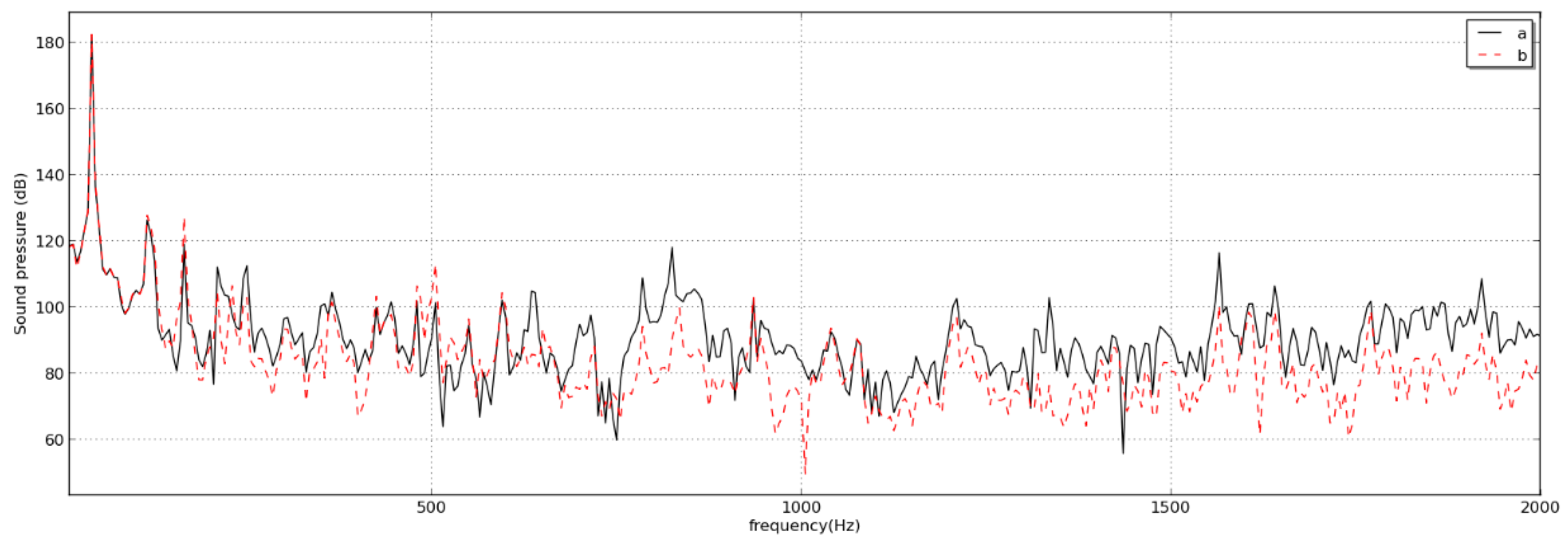
The sound pressure levels of points a and b, and those of points i and j are shown in Figure 11 and Figure 12, respectively.
The curve of the sound pressure level at point a is similar to that at point b in Figure 11, but the sound pressure level of point b is higher than that of point a in the low-frequency range. Point b is located more closely to the path of the horseshoe vortex than point a, and the strength of the excitation from the flow is more intense. The same laws can also be found at points c, d, e and f, which show that the flow-induced noise at the leading edge of the sail hull is mostly excited by the horseshoe vortex.
The sound pressure level at point i is lower than that of point j in the low- frequency range in Figure 12. The reason is that point j is closer to the path of the horseshoe vortex than point i, and the scale of the horseshoe vortex is large. With the increase of the frequency, the sound pressure level of point i is higher than that of point j, because point i is closer to the positions of the boundary layer separation and the tail vortex shedding than point j. Besides, the scale of the vortices of the boundary layer separation and the tail vortex shedding is smaller, compared to that of the horseshoe vortex. Then, the total sound pressure level of point i is higher than that of point j in the high-frequency range. The same laws can also be observed at points k, l, m and n, which show that the trailing edge of the sail hull is weakly excited by the horseshoe vortex since the horseshoe vortex dissipates at the trailing edge. The flow-induced noise at the trailing edge is dominated by the boundary layer separation and the tail vortex shedding, and thus, the tail vortex shedding generates the tone noise.
5.3. Analysis of Sound Radiation in the Far-Field
The curve of sound radiation power is shown in Figure 13. Some peaks are seen in the low-frequency range. With the increase of the frequency, the level of sound radiation power decreases. More specifically, the largest peak of sound radiation power level occurs at the frequency of f = 45 Hz, and the second largest peak is located at the frequency of 210 Hz. The two peaks can be considered as the flow-induced noise from the resonance mode of the model, which is excited by the horseshoe vortex. The peak of the frequency of 595 Hz is the flow-induced noise from the excitation of the tail vortex shedding, according to Equation (24). At the trailing edge of the sail hull, the contribution to the flow-induced noise by the excitation of the horseshoe vortex becomes weak.
The near sound field of the model is affected by the backflow of sound energy, which creates the differences between the sound radiation in the near field and that in the far field.
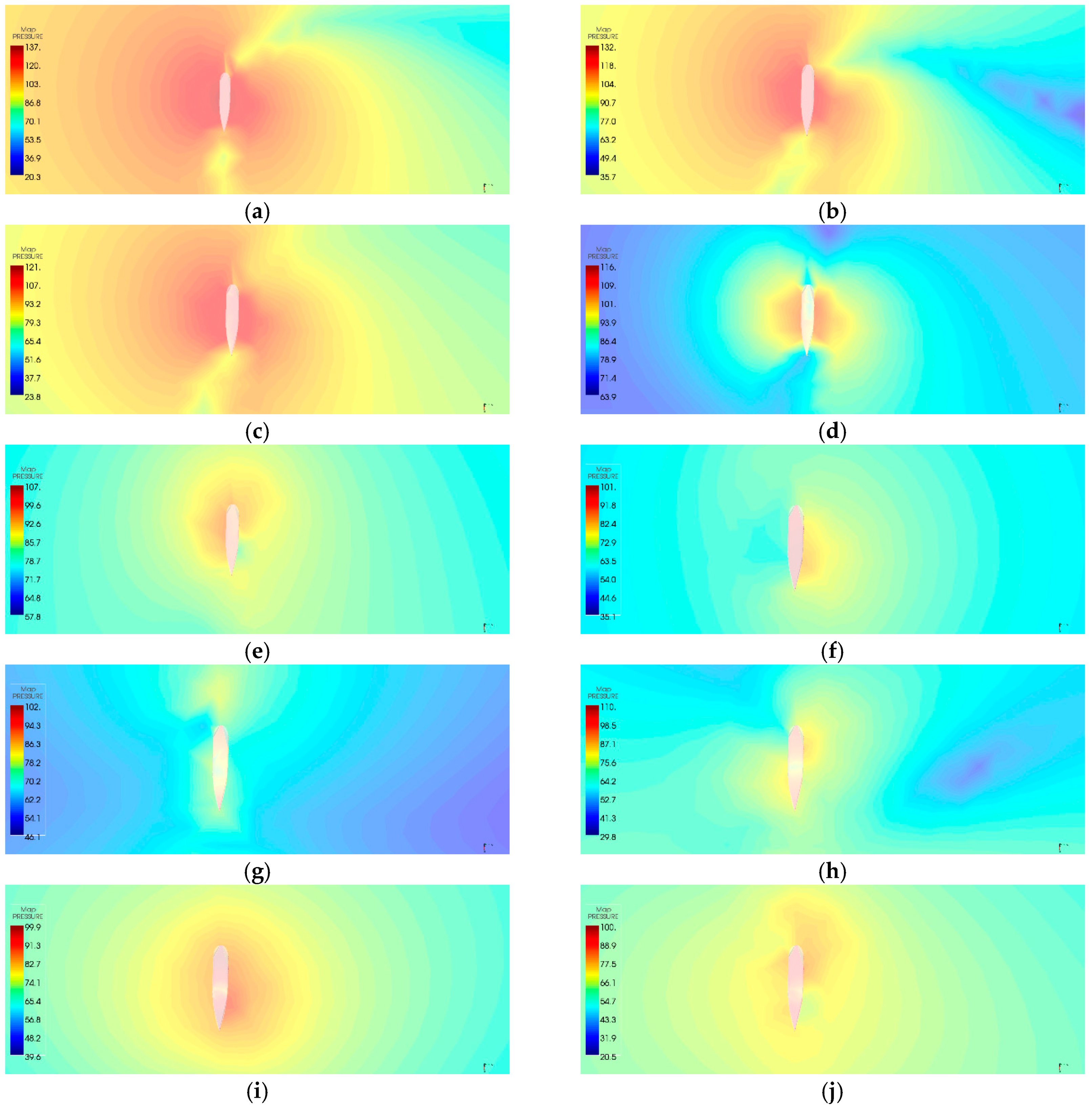
5.4. Contour of Sound Pressure of the Model
The contour of sound pressure at plane A is shown in Figure 14. The distributions of the sound field at different frequencies are approximately symmetrical with the chord of the sail hull. Because the primary source of the flow-induced noise in the low-frequency range is the horseshoe vortex, which has a large scale, and the distribution of the turbulent fluctuation pressure is roughly symmetrical to the chord of the sail hull. With the increase of the frequency, the distribution of the sound field of the sail hull becomes complicated. The boundary layer separation and the tail vortex shedding are ascribed to the sail hull excited to generate the flow-induced noise in the high-frequency range, and the structure of the vortices from the two flow phenomena is interlaced and not symmetrical to the chord of the sail hull. Therefore, the distribution of sound pressure is not entirely symmetrical to the chord of the sail hull.
5.5. Directivity of Sound Radiation
Figure 15 shows the horizontal directivities of the sound field of the sail hull at f = 10 Hz, 50 Hz, 100 Hz. At these lower frequencies, the sound radiation of the sail hull has the same horizontal directivity, the sound field is not symmetrical to the chord, and the angle with the intensive radiated noise is in the range from 45° to 135°.
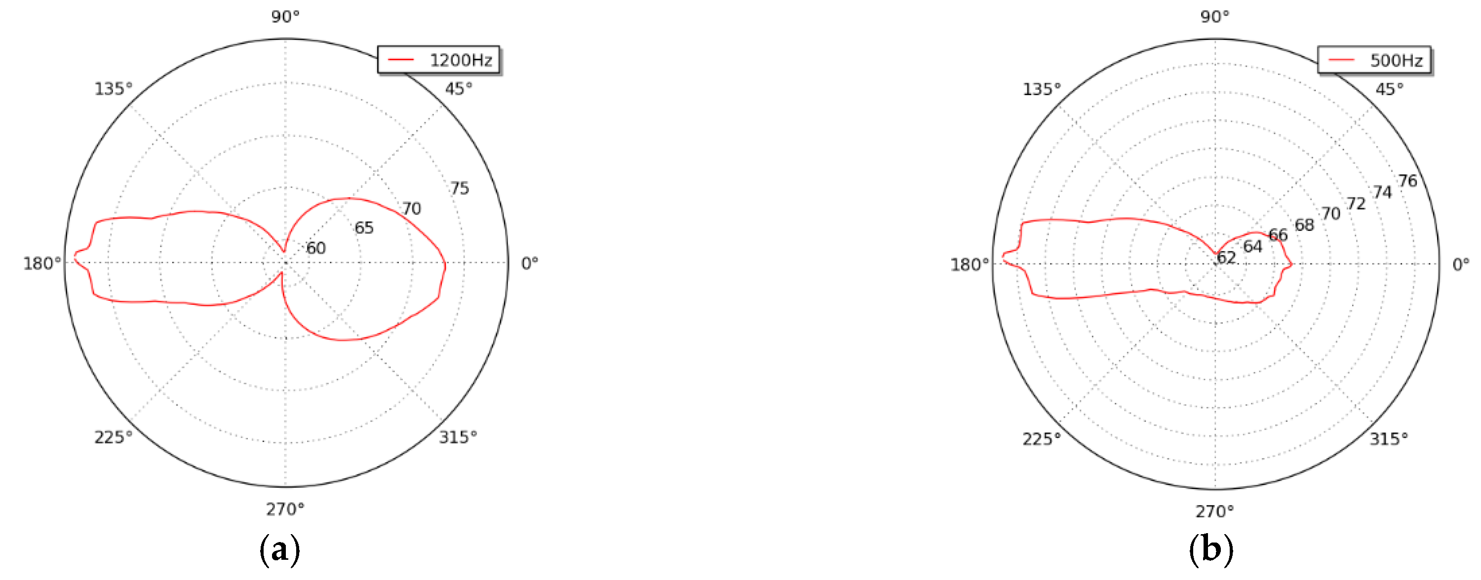
The horizontal directivity of the sail hull in high-frequency range is shown in Figure 16. The leading edge of the sail hull is mainly excited by the horseshoe vortex, which contributes very little to the flow-induced noise in the high-frequency range. The trailing edge of the sail hull is mainly excited by the tail vortex shedding, which contributes much to the flow-induced noise at a specific frequency. Besides, the boundary layer separation contributes mostly to the flow-induced noise in the high-frequency range. Since the boundary layer separation is variable in the process of the laminar flow to the turbulent flow, the horizontal directivity of the sail hull in the high-frequency range is not symmetrical, but with change, and cannot be summarized by some laws.
5.6. Comparison of Sound Radiation from the Two Kinds of the Sail Hulls
The horizontal directivity of the sail hull is different from that of the isolated sail hull, of which the submarine body is not considered. Therefore, we have also investigated the difference of sound radiation between two kinds of the sail hulls.
The isolated sail hull based on the SUBOFF model is established with the ratio of 1:48. Based on the established method of flow field calculation and sound field calculation, the curves of sound radiation power of the isolated sail hull and the sail hull in our study are shown in Figure 17. The flow-induced noise calculated by the sail hull in this research decreases with the increase of the frequency, while that of the isolated sail hull in the low-frequency range is notably lower. The isolated sail hull can only contain two types of unstable flow phenomena, the boundary layer separation and the tail vortex shedding. The unstable flow of the horseshoe vortex is ignored since the submarine body is not considered.
In the high-frequency range, the isolated sail hull is not embedded by the submarine body, which is equivalent to a free state. The tail vortices periodically fall off from the trailing edge of the sail hull, which excites the sail hull to generate the sound radiation power with several peaks. However, the frequency of the tail vortex shedding calculated by Equation (24) can only be a specific value, which is shown in Figure 13, in Section 5.3. Therefore, the flow-induced noise of the isolated sail hull is entirely different from that of the sail hull in the adopted model in our study. In addition, the model of the sail hull with part of submarine body can catch the unstable flow phenomenon of the horseshoe vortex from the triangular zone, and also be embedded by the submarine body, so that the simplified model in this research can provide more details for the research of the properties of sound radiation from the sail hull.
6. Experimental Validation of the Model
Based on the dimension of the model in the simulation, we have designed an experimental model to further analyze the properties of the flow-induced noise and have validated the results of numerical simulation. The measurement of the experimental model has been done in the gravity water tunnel in Harbin Engineering University. The hydrodynamic noise is measured by the reverberation method.
6.1. Theory of Reverberation Method
If a complex underwater sound source is placed in the free environment, the mean square sound pressure at a distance, r, from the sound source is:
where W0 is the sound radiation power, Pe is the effective sound pressure, is the density, and c0 is the sound velocity.
If the same sound source is placed in the reverberation tank, the mean square sound pressure is:
where is a constant of the reverberation tank, and is the coefficient of sound attenuation. Since the coefficient of sound attenuation in the water medium is smaller than the coefficient in the boundaries of the reverberation tank, the coefficient of sound attenuation in the water medium can be ignored.
The sound radiation power of the sound source in the far field can be expressed as:
Through the comparison of Equation (26) and Equation (27), we obtain:
Then,
where is the sound pressure level of the sound source, is the sound pressure level of spatial average in the reverberation area, and is a correction factor, which represents the difference of the sound pressure level between the spatial average measured in the reverberation field and the free field. The difference of the level can also be written as:
where , T60 is the reverberation time, and V is the total volume of the reverberation tank.
6.2. Description of the Experimental Measurement
The diagram of the experimental measurement and the photo of the model are shown in Figure 18.
The model is fixed at the bottom of the working section in the gravity water tunnel. The material of the cover plate in the working section is steel, and the other three sides are made of organic glass, which is of high sound permeability. A large water tank made of thick steel plate and tempered glass surrounds the working section to form a reverberation tank. The size is 4 × 3 × 4 m3. The hydrodynamic noise of the model in the working section is measured by the reverberation method in the reverberation control area with spatial average. The advantage of the reverberation method is that the hydrophone is placed in the still water, and the direct impact of the water flow on the hydrophone is avoided, because the direct impact of the flow enhances the background noise greatly and reduces the signal-to-noise ratio.
6.3. Results of the Experimental Measurement
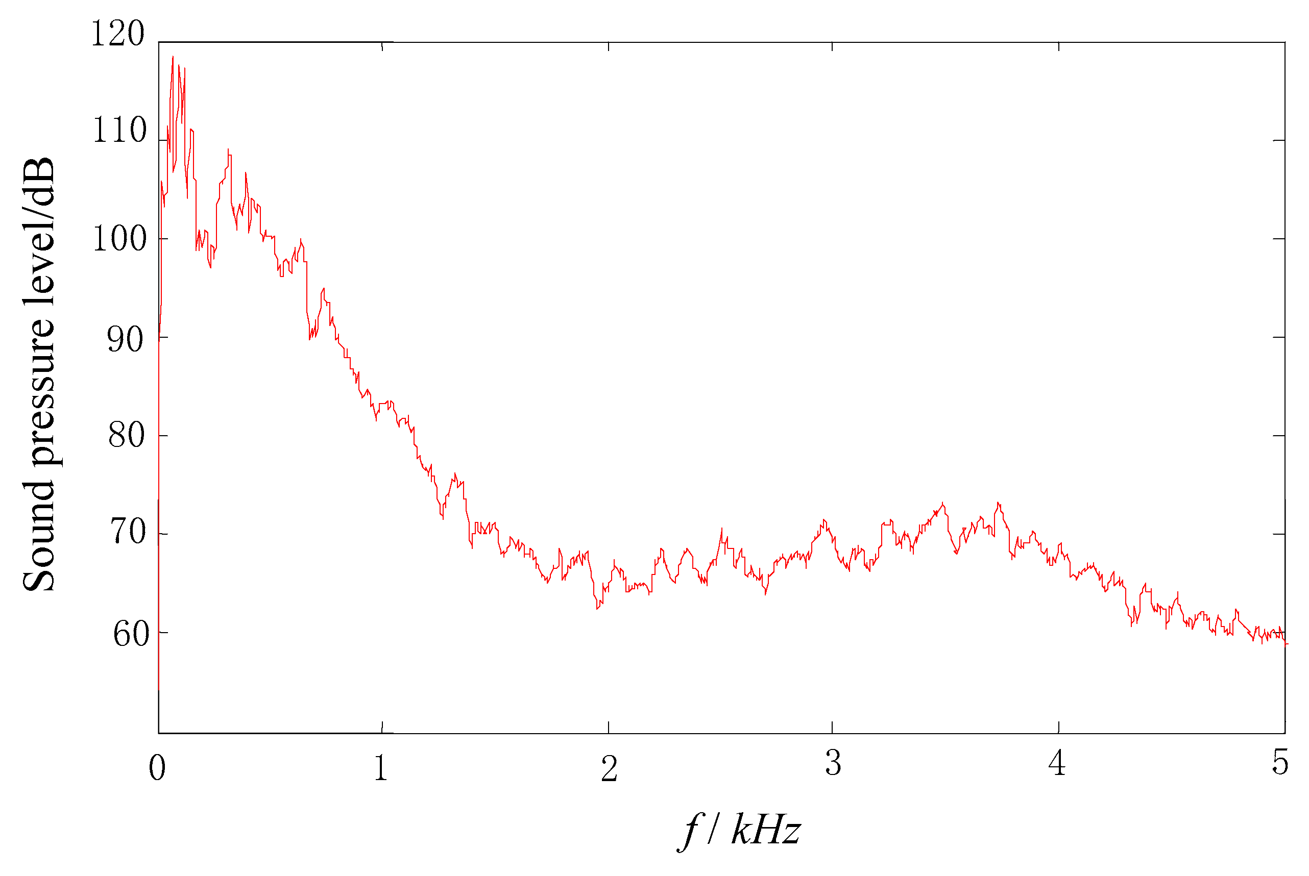
The change of the numbers of the opening valves in the gravity water tunnel at the outlets can achieve the velocities of the flow. The level of sound radiation power of the hydrodynamic noise from the model is shown in Figure 19. Some conclusions can be drawn:
(1) The high peaks of sound radiation power are mainly concentrated in the low-frequency range, which shows that the flow-induced noise induced by the horseshoe vortex is confirmed in the experiment.
(2) The level of sound radiation power in the low-frequency range is greater than that in the high-frequency range, and with the increase of the frequency, the change of sound radiation power is relatively mild, which shows that the flow-induced noise of the model excited by the boundary layer separation is measured in the experiment.
(3) At the frequency of 550 Hz, the peak shows that the model is excited by the tail vortex shedding measured in the experiment.
Therefore, the results in the experimental measurement validate the analysis in the numerical calculation.
However, some differences between the measurement and the calculation can be observed. The total level of sound radiation power from the model in the experiment is 119.47 dB, while that in the calculation is 113.52 dB. Some reasons may be ascribed to the difference made.
(1) Because the level of the flow noise is much lower than that of the flow-induced noise, the effect of the flow noise on the measurement can be ignored. However, the system of the gravity water tunnel is very similar to a long sound guide. Two tanks are at both ends of the gravity water tunnel, the formation of the design can make the flow-induced noise reflect many times, which enhances the level of the flow-induced noise. Even if we have calibrated the gravity water tunnel by a standard sound source, the effect of the reflection of the flow-induced noise cannot be accurately quantified since the process of the generation of the flow-induced noise is too complicated.
(2) In the numerical calculation, the wall surface of the flow field is set up as the boundary of the solid wall. However, the wall surface cannot meet the solid wall boundary in the experiment, especially in the water.
(3) The model in the experiment is made up of copper, and weld at the boundaries, which is different from the model in the simulation, and the latter is established completely and has no weld points.
(4) The background noise may interfere with the level of the hydrodynamic noise. Since the cavitation usually occurs, the velocity of the flow cannot be made too high, and the signal-to-noise ratio is relatively low.
Besides, the hydrodynamic noise is a random process. All these factors make the experimental results unable to match accurately with that of the numerical calculation.
7. Conclusions
We have taken the sail hull with part of the submarine body as the research model to investigate the generation mechanism of the hydrodynamic noise, especially the flow-induced noise from the sail hull. This complements the ignorance of the flow phenomenon of the horseshoe vortex in the isolated sail hull. The calculation of the flow field of the model is carried out by the method of LES. The unstable flow phenomena of the sail hull are analyzed. The turbulent fluctuation pressure is extracted as the excitation force from the flow field. Then, the sound radiation of the model is calculated by the wavenumber–frequency spectrum. After the simulation, the experimental validation has been done. Some conclusions can be drawn:
(1) The horseshoe vortex, the boundary layer separation, and the tail vortex shedding are ascribed to the three kinds of unstable flow phenomena in the sail hull.
(2) The flow-induced noise generated by the excitation of the horseshoe vortex is mainly in the low-frequency range. The flow-induced noise generated by the boundary layer separation exists in the whole frequency range. Only at the frequency of the tail vortex shedding, does the quasi-periodic excitation of the tail vortex produce the peaks of the flow-induced noise.
(3) With the joint effect of the horseshoe vortex and the boundary layer separation, the frequency spectrum of the flow-induced noise has several peaks. As the frequency increases, the contribution from the excitation of the horseshoe vortex decreases, so that the level of the flow-induced noise decreases continuously. At the trailing edge of the sail hull, the strength of the horseshoe vortex decays. When the tail vortex passing through the model coincides with the characteristic frequency of the tail vortex shedding, a high peak of the flow-induced noise is formed in the frequency range. Therefore, the radiated noise spectrum of the sail hull is manifested by the tones and the continuous broadband.
(4) The sound pressure on the surface of the sail hull is decreased from the leading edge to the trailing edge. Outside of the position of the horseshoe vortex, the fluctuation pressure generated by the boundary layer separation is relatively uniform, which makes the distribution of the flow-induced noise on the surface of the sail hull more uniform. The tail vortex shedding occurs at the trailing edge of the sail hull, which makes the distribution of the flow-induced noise on the surface of the sail hull further intensive.
(5) In the low-frequency range, the sound radiation of the sail hull is approximately symmetrical to the direction of the chord, and the angle of horizontal directivity is more intensive in the range from 45° to 135°. With the increase of the frequency, the distribution of the radiated sound field of the sail hull becomes complicated. However, the bow and the tail of the model are still the intensive positions of the flow-induced noise.
(6) The measurement of the hydrodynamic noise is carried out in the gravity water tunnel, based on the reverberation method. The peaks of the frequency spectrum agree approximately with the simulation, which further validates the accuracy of the numerical calculation and the analysis from the numerical simulation.
These results can provide reference for the design of flow control devices under various kinds of unstable flow phenomena and the reduction of flow-induced noise. At the same time, the results in this study compensate for the shortcomings of past research on the sound field properties of the isolated sail hull, providing a more accurate method for the calculation of the sail hull’s flow-induced noise. In the future, based on the results of this research, some methods of the unstable flow change can be used to reduce the flow-induced noise of the sail hull, of which the relevant validations can be carried out in experimental tests.
Author Contributions
Writing of the original draft preparation, Y.L. (Yalin Li); writing of review and editing, Y.L. (Yongwei Liu); supervision, D.S.
Funding
This research was funded by the steady support plan from the Acoustic Science and Technology Laboratory (grant number: SSJSWDZC2018005), the project from the Key Laboratory of Acoustic Stealth (grant number: 614220405011706), and the fundamental research funds for central universities (grant number: HEUCF180503).
Acknowledgments
The author would like to thank Peichun Amy Tsai for kind help.
Conflicts of Interest
The authors declare no conflicts of interest.
References
- Kwon, H.W.; Hong, S.Y.; Song, J.H. Energy flow models for underwater radiation noise prediction in medium-to-high-frequency ranges. J. Eng. Marit. Environ. 2015, 230, 404–416. [Google Scholar] [CrossRef]
- Caresta, M.; Kessissoglou, N.J. Acoustic signature of a submarine hull under harmonic excitation. Appl. Acoust. 2010, 71, 17–31. [Google Scholar] [CrossRef]
- Mousavi, B.; Rahrovi, A.A.; Kheradmand, S. Numerical simulation of tonal and broadband hydrodynamic noises of non-cavitating underwater propeller. Pol. Marit. Res. 2014, 21, 46–53. [Google Scholar] [CrossRef]
- Zhihua, L.; Ying, X.; Chengxu, T. Method to control unsteady force of submarine propeller based on the control of horseshoe vortex. J. Ship Res. 2012, 56, 12–22. [Google Scholar] [CrossRef]
- Huo, L.; Fei, S.M. Design on the fairwater shape and its influence on the radiation noise of submarines. J. Vibroeng. 2016, 18, 1392–8716. [Google Scholar] [CrossRef]
- Liu, Z.H.; Xiong, Y.; Tu, C.X. The method to control the submarine horseshoe vortex by breaking the vortex core. J. Hydrodyn. 2014, 26, 637–645. [Google Scholar] [CrossRef]
- Porteous, R.; Moreau, D.J.; Doolan, C.J. A review of flow-induced noise from finite wall-mounted cylinders. J. Fluids Struct. 2014, 51, 240–254. [Google Scholar] [CrossRef]
- da Rocha, J.; Suleman, A.; Lau, F. Flow-induced noise and vibration in aircraft cylindrical cabins: Closed-form analytical model validation. J. Vib. Acoust. 2011, 133, 051013. [Google Scholar] [CrossRef]
- Kudashev, E.B.; Kolyshnitsyn, V.A.; Marshov, V.P.; Tkachenko, V.M.; Tsvetkov, A.M. Experimental simulation of hydrodynamic flow noises in an autonomous marine laboratory. Acoust. Phys. 2013, 59, 187–196. [Google Scholar] [CrossRef]
- Abshagen, J.; Schäfer, I.; Will, C.; Pfister, G. Coherent flow noise beneath a flat plate in a water tunnel experiment. J. Sound Vib. 2015, 340, 211–220. [Google Scholar] [CrossRef]
- Kang, H.; Tsutahara, M. An application of the finite difference-based lattice Boltzmann model to simulating flow-induced noise. Int. J. Numer. Methods Fluids 2006, 53, 629–650. [Google Scholar] [CrossRef]
- Zhang, N.; Xie, H.; Wang, X.; Wu, B.S. Computation of vertical flow and flow induced noise by large eddy simulation with FW-H acoustic analogy and Powell vortex sound theory. J. Hydrodyn. 2016, 28, 255–266. [Google Scholar] [CrossRef]
- Liu, K.; Zhou, S.; Li, X.; Shu, X.; Guo, L.; Li, J.; Zhang, X. Flow-induced noise simulation using detached eddy simulation and the finite element acoustic analogy method. Adv. Mech. Eng. 2016, 8, 1–8. [Google Scholar] [CrossRef]
- Qu, D.; Zhang, Z.; Lou, J. Analysis of hydrodynamic noise characteristics of rudder-wing. J. Vibroeng. 2017, 11, 2345–2533. [Google Scholar] [CrossRef]
- Li, X.-G.; Yang, K.-D.; Ma, Y.-L. Flow-noise calculation using the mutual coupling between vulcanized rubber and the flow around in water. Chin. Phys. Lett. 2012, 29, 064301. [Google Scholar] [CrossRef]
- MÖzden, M.C.; Gürkan, A.Y.; Özden, Y.A.; Canyurt, T.G.; Korkut, E. Underwater radiated noise prediction for a submarine propeller in different flow conditions. Ocean Eng. 2016, 126, 488–500. [Google Scholar] [CrossRef]
- Wei, Y.S.; Wang, Y.S.; Chang, S.P.; Jian, F. Numerical prediction of propeller excited acoustic response of submarine structure based on CFD, FEM and BEM. J. Hydrodyn. 2016, 24, 207–216. [Google Scholar] [CrossRef]
- Doolan, C.J.; Moreau, D.J. Flow-induced noise generated by sub-boundary layer steps. Exp. Therm. Fluid Sci. 2016, 72, 47–58. [Google Scholar] [CrossRef]
- Moreau, D.J.; Prime, Z.; Porteous, R.; Doolan, C.J.; Valeau, V. Flow-induced noise of a wall-mounted finite airfoil at low-to-moderate Reynolds number. J. Sound Vib. 2014, 333, 6924–6941. [Google Scholar] [CrossRef]
- Zhu, W.J.; Shen, W.Z.; Sørensen, J.N. High-order numerical simulations of flow-induced noise. Int. J. Numer. Methods Fluids 2011, 66, 17–37. [Google Scholar] [CrossRef]
- Prek, M. The impact of geometrical parameters on hydrodynamic noise generation. Appl. Acoust. 2000, 60, 343–351. [Google Scholar] [CrossRef]
- von Benda-Beckmann, A.M.; Wensveen, P.J.; Samarra, F.I.; Beerens, S.P.; Miller, P.J. Correction: Separating underwater ambient noise from flow noise recorded on stereo acoustic tags attached to marine mammals. J. Exp. Biol. 2016, 219, 2271–2275. [Google Scholar] [CrossRef] [PubMed]
- Barker, S.J. Measurements of hydrodynamic noise from submerged hydrofoils. J. Acoust. Soc. Am. 1976, 59, 1095–1103. [Google Scholar] [CrossRef]
- Kaltenbacher, M.; Escobar, M.; Becker, S.; Ali, I. Numerical simulation of flow-induced noise using LES/SAS and Lighthill’s acoustic analogy. Int. J. Numei. Meth. Fluids 2010, 63, 1103–1122. [Google Scholar] [CrossRef]
- Germano, M.; Piomelli, U.; Moin, P.; Cabot, W.H. A dynamic subgrid-scale eddy viscosity model. Phys. Fluids 1991, 3, 1760–1765. [Google Scholar] [CrossRef]
- Groves, N.C.; Huang, T.T.; Chang, M.S. Geometric Characteristics of DARPA SUBOFF Models; David Taylor Research Center, Bethesda, USA: Rockville, MD, USA, 1989; pp. 1–51. [Google Scholar]
- Heatwole, C.M.; Franchek, M.A.; Bernhard, R.J. A robust feedback controller implementation for flow induced structural radiation of sound. In Proceedings of the INTER-NOISE and NOISE-CON Congress and Conference, Seattle, WA, USA, 29 September–2 October 1996; Institute of Noise Control Engineering: Reston, VA, USA, 1996. [Google Scholar]
- Zhang, N.; Shen, H.; Zhu, X.; Yao, H.Z.; Xie, H. Numerical simulation on the effect of fairwater optimization to suppress the wall pressure fluctuations and flow induced noise. J. Ship Mech. 2014, 4, 448–458. [Google Scholar] [CrossRef]
- Huang, Q. A Numerical Study of the Flow around Airfoils with Serrated Trailing Edges and the Aerodynamic Noise Based on Large Eddy Simulation. Ph.D. Thesis, Tsinghua University, Beijing, China, 2015. [Google Scholar]
Figure 1.
Diagram of the model. The model is the sail hull with part of the submarine body, which is scaled from the SUBOFF model. The length (L), and the height (h) of the sail hull are 1.84 m, and 0.1 m, respectively. The chord length (c) is 0.184 m.
Figure 1.
Diagram of the model. The model is the sail hull with part of the submarine body, which is scaled from the SUBOFF model. The length (L), and the height (h) of the sail hull are 1.84 m, and 0.1 m, respectively. The chord length (c) is 0.184 m.

Figure 2.
Comparison of the tail flow from the SUBOFF between the numerical calculation and experimental test. Numerical calculation: (a) y+ < 50; (b) y+ < 100; (c) y+ < 250; and (d) y+ < 300. (e) The experimental test.
Figure 2.
Comparison of the tail flow from the SUBOFF between the numerical calculation and experimental test. Numerical calculation: (a) y+ < 50; (b) y+ < 100; (c) y+ < 250; and (d) y+ < 300. (e) The experimental test.

Figure 3.
Comparison of results between the experimental test and numerical simulation. The dark line shows the results of the preliminary test, and the red line shows the results of numerical calculation. The horizontal axis denotes the frequency in the range from 0 to 1 kHz, and the longitudinal axis indicates the sound pressure level with a reference of 20 μPa.

Figure 4.
Diagram of the reference planes. Plane A is in the longitudinal direction, plane B is also in the longitudinal direction, which is perpendicular to plane A, and plane C is in the transverse direction.
Figure 4.
Diagram of the reference planes. Plane A is in the longitudinal direction, plane B is also in the longitudinal direction, which is perpendicular to plane A, and plane C is in the transverse direction.
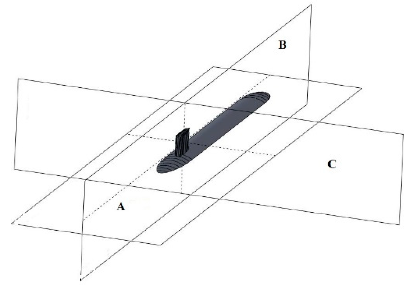
Figure 5.
Pressure contours at different reference planes: (a) plane A; and (b) plane B. The pressure gradient is adverse when the points are approaching the leading edge.
Figure 5.
Pressure contours at different reference planes: (a) plane A; and (b) plane B. The pressure gradient is adverse when the points are approaching the leading edge.

Figure 6.
Contours of the flow field at plane A: (a) pressure contour; (b) velocity contour; and (c) kinetic turbulent energy.
Figure 6.
Contours of the flow field at plane A: (a) pressure contour; (b) velocity contour; and (c) kinetic turbulent energy.

Figure 7.
Flow phenomena of the two models: (a) the adopted model in this research; and (b) the isolated sail hull.
Figure 7.
Flow phenomena of the two models: (a) the adopted model in this research; and (b) the isolated sail hull.

Figure 8.
Diagram of the streamline at the trailing edge of the sail hull at different times: (a) 0.3125 s; (b) 0.625 s; (c) 0.9375 s; (d) 1.25 s; (e) 1.5625 s; (f) 1.875 s; (g) 2.1875 s; and (h) 2.5 s.
Figure 8.
Diagram of the streamline at the trailing edge of the sail hull at different times: (a) 0.3125 s; (b) 0.625 s; (c) 0.9375 s; (d) 1.25 s; (e) 1.5625 s; (f) 1.875 s; (g) 2.1875 s; and (h) 2.5 s.
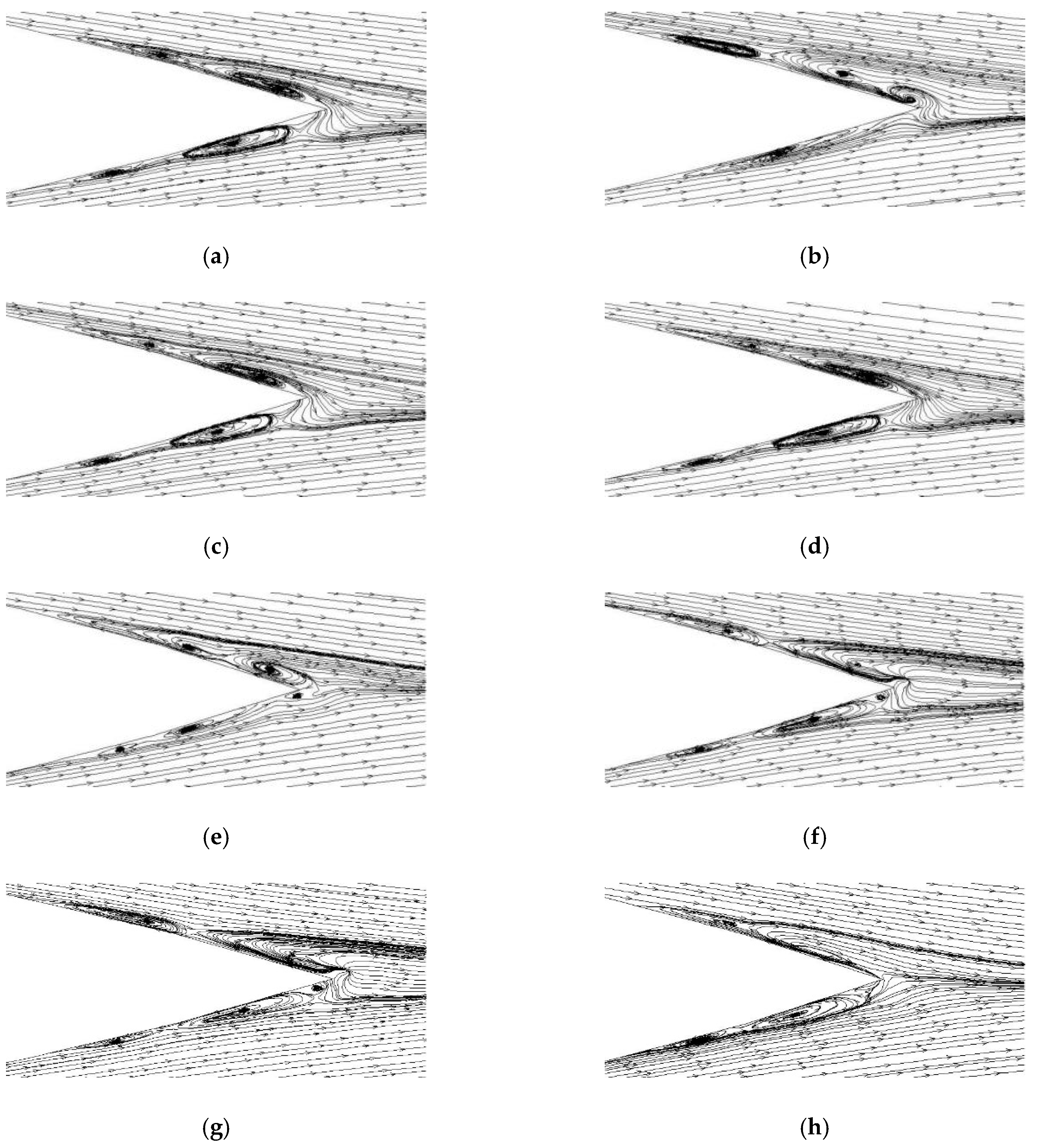
Figure 9.
Distribution of the fluctuation pressure on the surface of the model at different frequencies: (a) f = 50 Hz; (b) f = 200 Hz; (c) f = 400 Hz; (d) f = 600 Hz; (e) f = 800 Hz; (f) f = 1000 Hz; (g) f = 1600 Hz; and (h) f = 2000 Hz. The left color bar shows the magnitude of the fluctuation pressure.
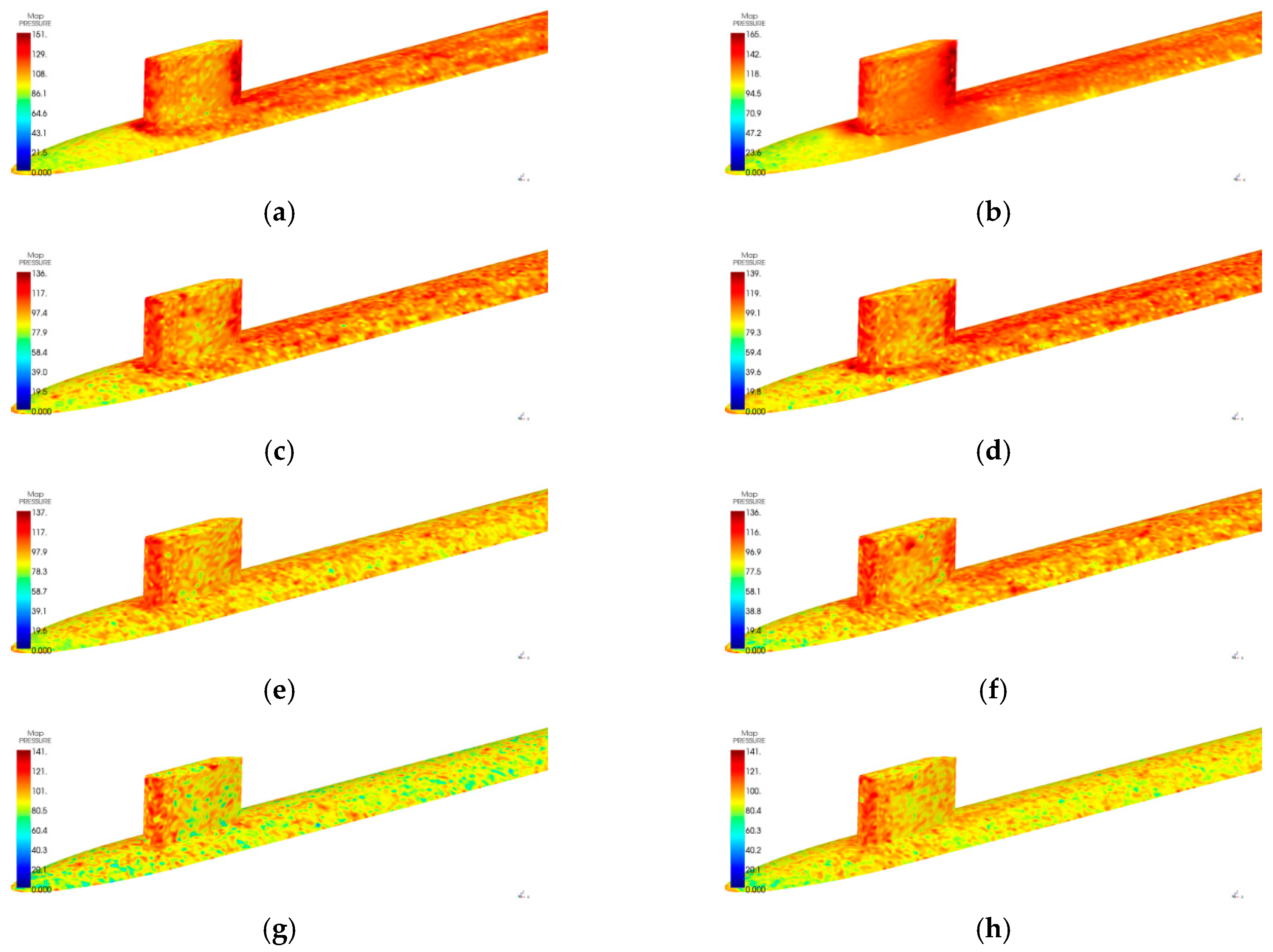
Figure 10.
Locations of the field points. Points a, c, e, g, i, k, and m are located at the middle height of the sail hull. Points b, d, f, h, j, l, and n are located at the junction between the sail hull and the submarine body.
Figure 10.
Locations of the field points. Points a, c, e, g, i, k, and m are located at the middle height of the sail hull. Points b, d, f, h, j, l, and n are located at the junction between the sail hull and the submarine body.
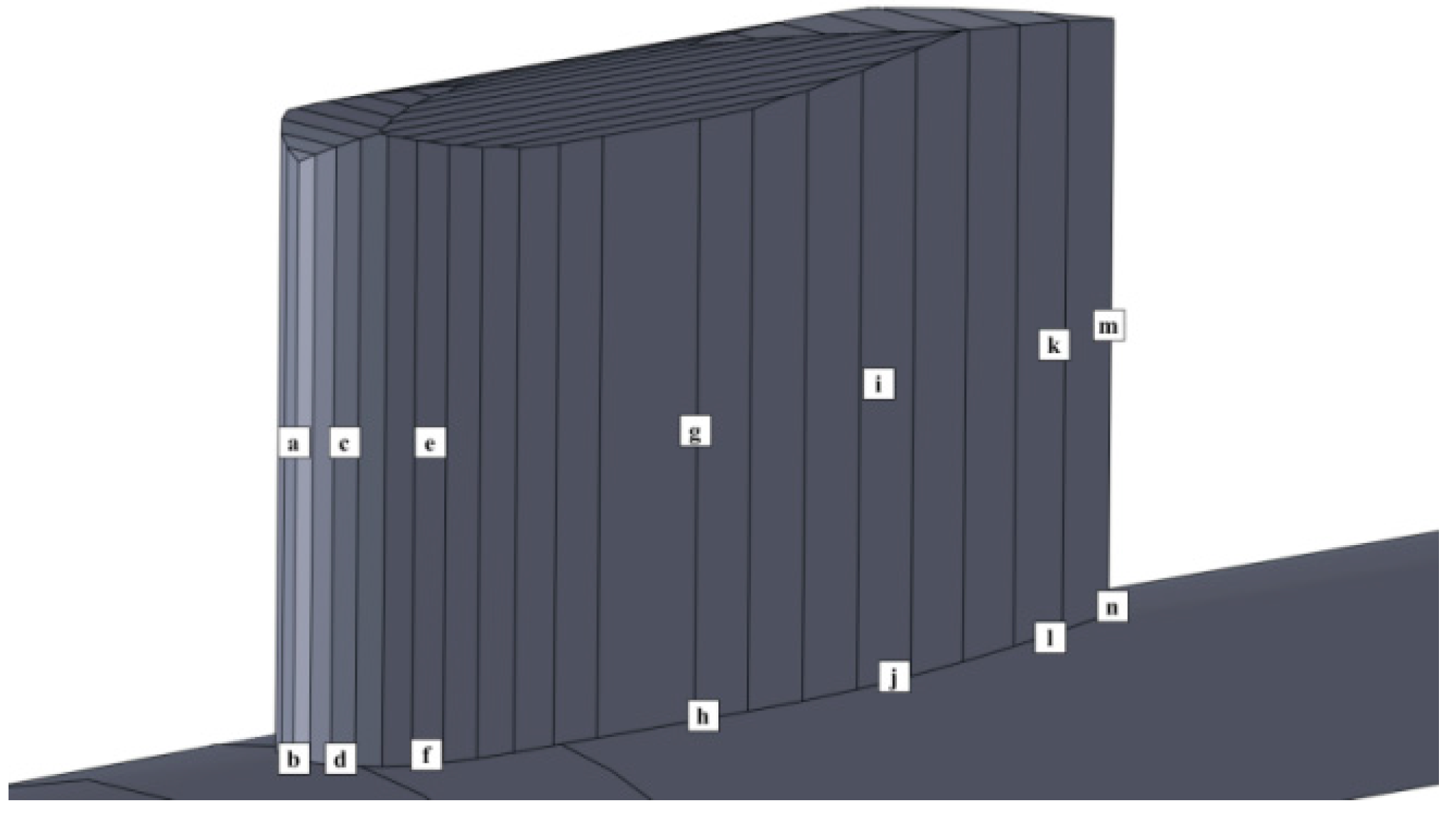
Figure 11.
Curves of sound pressure levels from points a and b. The continuous black line denotes the sound pressure level of point a, while the red dot line denotes the sound pressure level of point b.
Figure 11.
Curves of sound pressure levels from points a and b. The continuous black line denotes the sound pressure level of point a, while the red dot line denotes the sound pressure level of point b.

Figure 12.
Curves of sound pressure levels from points i and j. The continuous black line denotes the sound pressure level of point i, while the red dot line denotes the sound pressure level of point j.
Figure 12.
Curves of sound pressure levels from points i and j. The continuous black line denotes the sound pressure level of point i, while the red dot line denotes the sound pressure level of point j.

Figure 13.
Sound radiation power of the sail hull. In the low-frequency range, some peaks can easily be observed, while in the high-frequency range, the curve of the sound radiation power is rather continuous.
Figure 13.
Sound radiation power of the sail hull. In the low-frequency range, some peaks can easily be observed, while in the high-frequency range, the curve of the sound radiation power is rather continuous.
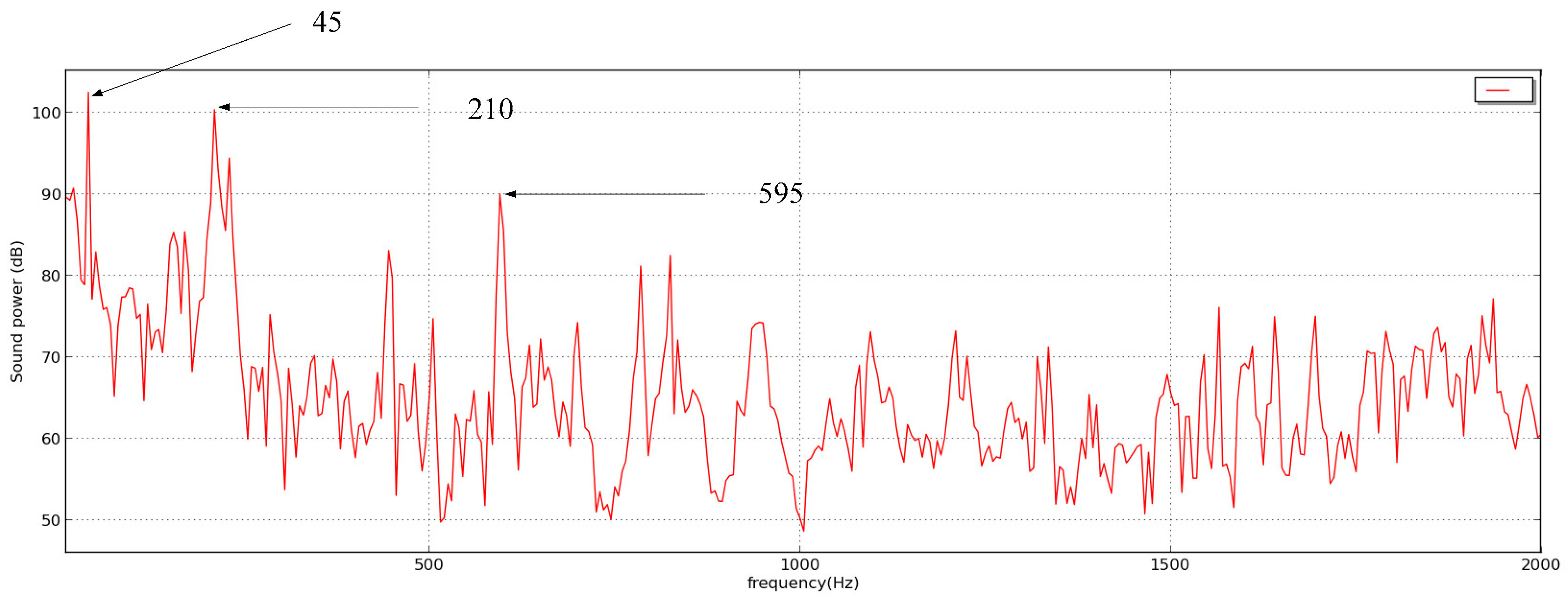
Figure 14.
Contour of sound pressure of the sail hull: (a) f = 10 Hz; (b) f = 50 Hz; (c) f = 100 Hz; (d) f = 150 Hz; (e) f = 200 Hz; (f) f = 600 Hz; (g) f = 800 Hz; (h) f = 1200 Hz; (i) f = 1800 Hz; and (j) f = 2000 Hz.
Figure 14.
Contour of sound pressure of the sail hull: (a) f = 10 Hz; (b) f = 50 Hz; (c) f = 100 Hz; (d) f = 150 Hz; (e) f = 200 Hz; (f) f = 600 Hz; (g) f = 800 Hz; (h) f = 1200 Hz; (i) f = 1800 Hz; and (j) f = 2000 Hz.

Figure 15.
Horizontal directivity of sound pressure of the sail hull in low-frequency range. The pink line denotes the frequency of 10 Hz. The red line denotes the frequency of 50 Hz. The black line denotes the frequency of 100 Hz.
Figure 15.
Horizontal directivity of sound pressure of the sail hull in low-frequency range. The pink line denotes the frequency of 10 Hz. The red line denotes the frequency of 50 Hz. The black line denotes the frequency of 100 Hz.
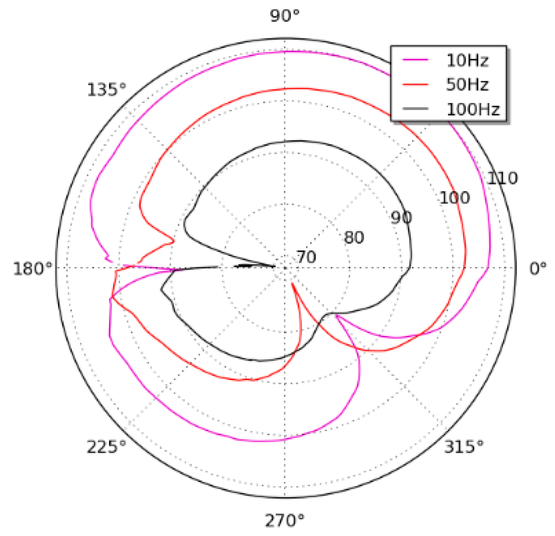
Figure 16.
Horizontal directivity of sound pressure of the sail hull in the high-frequency range: (a) f = 500 Hz; (b) f = 1200 Hz; (c) f = 1600 Hz; and (d) f = 2000 Hz.
Figure 16.
Horizontal directivity of sound pressure of the sail hull in the high-frequency range: (a) f = 500 Hz; (b) f = 1200 Hz; (c) f = 1600 Hz; and (d) f = 2000 Hz.

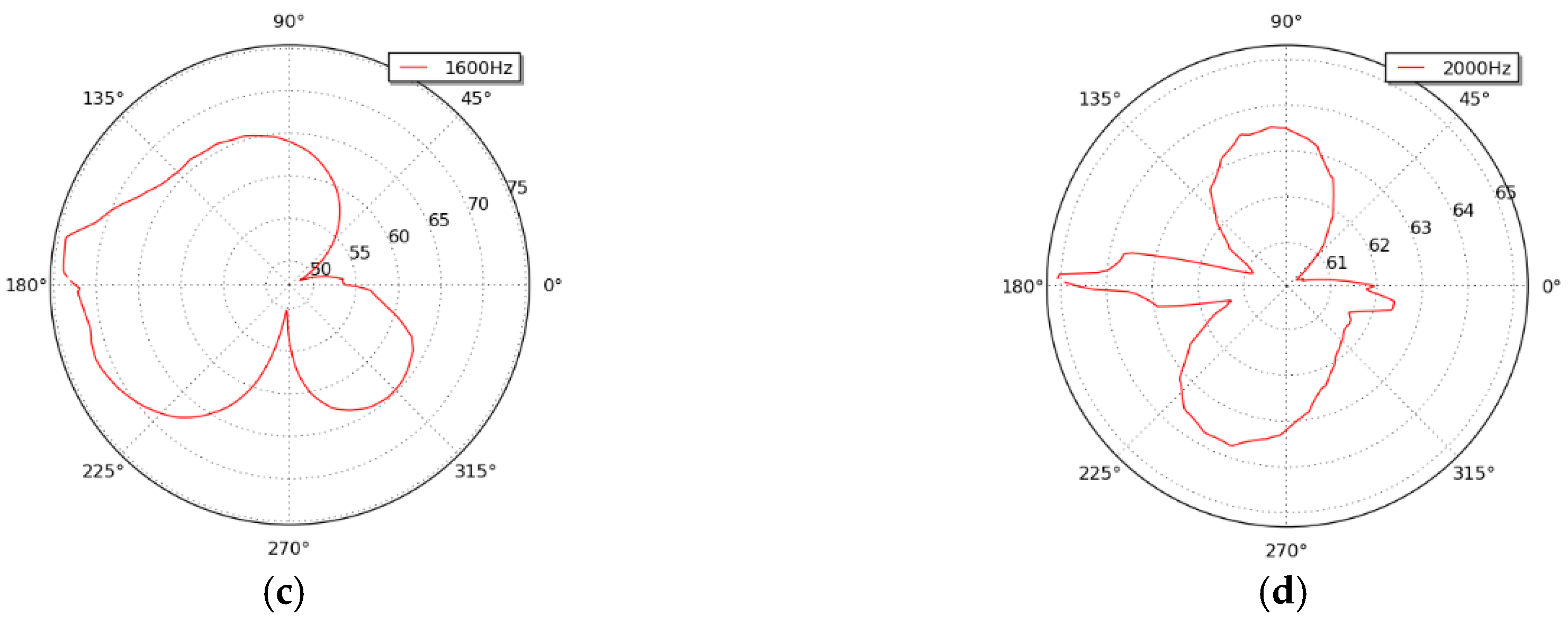
Figure 17.
Comparison between the sound radiation power from the sail hull in our study and the isolated sail hull. The red line denotes the sound radiation power from the sail hull in this research. The black dotted line denotes the sound radiation power from the isolated sail hull.
Figure 17.
Comparison between the sound radiation power from the sail hull in our study and the isolated sail hull. The red line denotes the sound radiation power from the sail hull in this research. The black dotted line denotes the sound radiation power from the isolated sail hull.
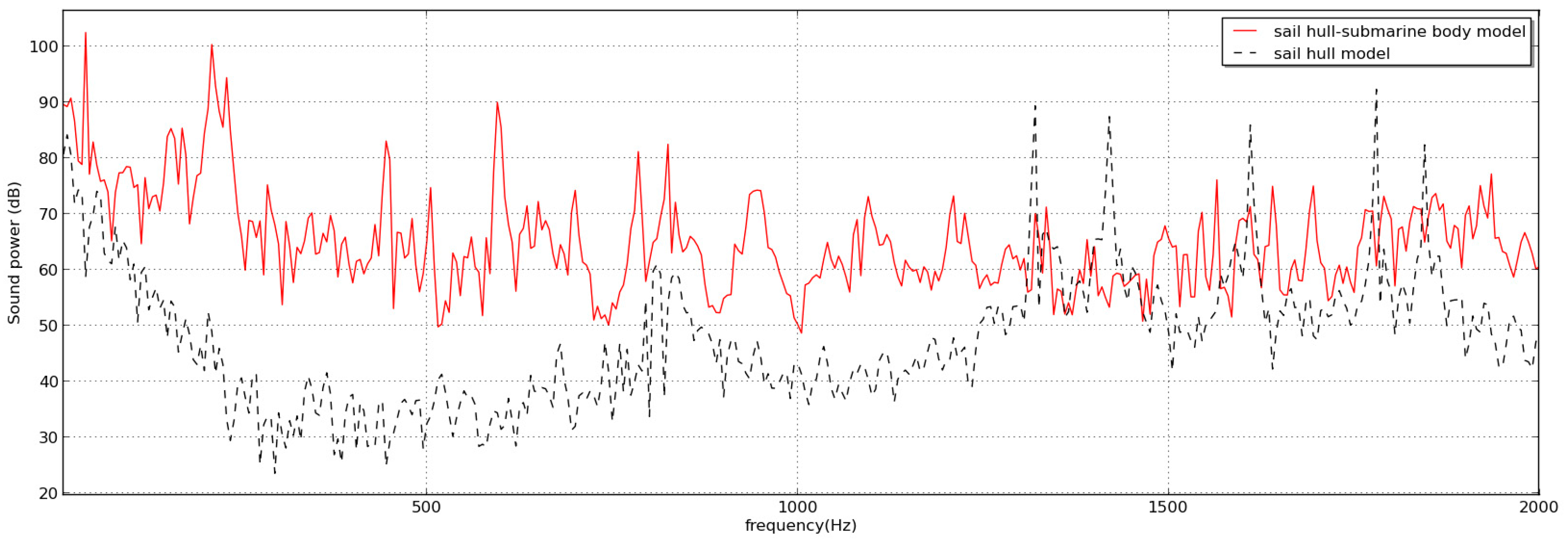
Figure 18.
Diagram of the measurement. (a) Chart of the experimental test. The model is rigidly placed at the bottom of the working section, and the hydrodynamic noise from the model is excited by the water flow due to the gravity. A vertical array of several hydrophones is placed in the water tank outside the working section, which collects the hydrodynamic noise from the model. (b) Practical photo of the model.
Figure 19.
Diagram of sound radiation power from the model in the experiments. The red line denotes the hydrodynamic noise from the model at a velocity of 8.68 m/s. The horizontal axis indicates the frequency range, while the vertical axis indicates the level of sound radiation power.
Figure 19.
Diagram of sound radiation power from the model in the experiments. The red line denotes the hydrodynamic noise from the model at a velocity of 8.68 m/s. The horizontal axis indicates the frequency range, while the vertical axis indicates the level of sound radiation power.


Table 1.
Resistance values of the models with different grid numbers.
| No. | Grid Numbers | Resistance Values |
|---|---|---|
| 1 | 1 million | 33.9004 |
| 2 | 1.5 million | 34.1862 |
| 3 | 2 million | 34.9821 |
| 4 | 2.5 million | 35.6891 |
| 5 | 3 million | 35.6893 |
| 6 | 3.5 million | 35.6979 |
| 7 | 4 million | 35.6986 |
Table 2.
Comparison of the resistance.
| y+ | Numerical Simulation Value | Experimental Test Value |
|---|---|---|
| <50 | 102.0 | 102.3 |
| <100 | 109.3 | 102.3 |
| <250 | 120.2 | 102.3 |
| <300 | 98.1 | 102.3 |
© 2018 by the authors. Licensee MDPI, Basel, Switzerland. This article is an open access article distributed under the terms and conditions of the Creative Commons Attribution (CC BY) license (http://creativecommons.org/licenses/by/4.0/).
Share and Cite
MDPI and ACS Style
Liu, Y.; Li, Y.; Shang, D. The Generation Mechanism of the Flow-Induced Noise from a Sail Hull on the Scaled Submarine Model. Appl. Sci. 2019, 9, 106. https://doi.org/10.3390/app9010106
AMA Style
Liu Y, Li Y, Shang D. The Generation Mechanism of the Flow-Induced Noise from a Sail Hull on the Scaled Submarine Model. Applied Sciences. 2019; 9(1):106. https://doi.org/10.3390/app9010106
Chicago/Turabian StyleLiu, Yongwei, Yalin Li, and Dejiang Shang. 2019. "The Generation Mechanism of the Flow-Induced Noise from a Sail Hull on the Scaled Submarine Model" Applied Sciences 9, no. 1: 106. https://doi.org/10.3390/app9010106
Note that from the first issue of 2016, this journal uses article numbers instead of page numbers. See further details here.