Exploiting the Underdetermined System in Multichannel Active Noise Control for Open Windows


1
Maxim Integrated, San Jose, CA 95134, USA
2
School of Electrical and Electronic Engineering, Nanyang Technological University, Singapore 639798, Singapore
*
Authors to whom correspondence should be addressed.
Appl. Sci. 2019, 9(3), 390; https://doi.org/10.3390/app9030390
Submission received: 18 November 2018
/
Revised: 11 January 2019
/
Accepted: 16 January 2019
/
Published: 23 January 2019
(This article belongs to the Special Issue Active and Passive Noise Control)
Abstract
:Active noise control (ANC) is a re-emerging technique to mitigate noise pollution. To reduce the noise power in large spaces, multiple channels are usually required, which complicates the implementation of ANC systems. In this paper, we separate the multichannel ANC problem into two subproblems, where the subproblem of computing the control filter is usually an underdetermined problem. Therefore, we could leverage the underdetermined system to simplify the ANC system without degrading the noise reduction performance. For a single incidence, we compare the conventional fully-coupled (pseudoinverse) multichannel control with the colocated (diagonal) control method and find that they can achieve equivalent performance, but the colocated control method is less computationally intensive. Furthermore, the underdetermined system presents an opportunity to control noise from multiple incidences with one common fixed filter. Both the full-rank and the overdetermined optimal control filters are realized. The performance of these control methods was analyzed numerically with the Finite Element Method (FEM) and the results validate the feasibility of the full-rank and overdetermined optimal control methods, where the latter could even offer more robust performance in more complex noise scenarios.
1. Introduction
Active noise control (ANC) mitigates disturbances by generating sound waves that interfere destructively with the primary noise field. The destructively interfering sound field is generated by secondary sources driven to minimize the sum-of-squared pressures at the error microphone locations [1]. Although ANC is widely implemented in headphones, it is only in recent years that ANC has been applied to control noise in larger 3D spaces, such as in infant incubators [2], the interior of automobiles [3,4], and through apertures [5,6].
In light of the increasing awareness of health risks associated with long-term exposure to environmental noise [7,8,9], sustainable noise mitigation methods need to be implemented to increase the aural comfort in affected urban accommodation. Because windows are the main entry points for environmental noise in a building, active mitigation methods are most effective when targeted at such openings. Since windows have to provide natural ventilation—especially in tropical climates—passive methods of control (e.g., double-glazed panels, barriers, etc.) are less favorable as they obstruct both sunlight and ventilation. Hence, ANC techniques that can mitigate noise through open windows are potentially sustainable solutions to environmental noise in tropical urban high-rise environments [10].
ANC systems have been developed and studied for fully-open [11,12,13,14,15,16,17], and partially-open windows [6,18,19,20]. For practical implementations, however, the requirement of error microphones in the system poses placement challenges, computation issues, and privacy concerns. Although global noise attenuation of around 10 dB has been demonstrated experimentally with a fixed set of control filter coefficients in some cases [11,12], the mechanism behind the formulation of a single filter, which is optimal for different noise scenarios (e.g., different incidence angles), has not been defined.
Whilst non-adaptive ANC systems that do not employ error microphones have been realized in a multi-dimensional reverberant room, the optimal filters used in such cases must be recalculated when the primary or secondary path transfer functions change (e.g., human movements in the room) [1]. However, if the window problem is formulated such that the total acoustic power transmitted through the window is the cost function to be minimized, the ANC performance will be robust to variations in the secondary path for optimal filters that do not employ error microphones [21]. This formulation also assumes that the window opening is the noise source, which is collocated with the reference microphones and secondary sources, yielding a favorable control scenario. Thus, optimal filters can be designed using the inversion method with free-field secondary path measurements for each window design (i.e., without room reverberations). The problem is how feasible it is to design such a fixed optimal filter that can work well in various scenarios of noise in open windows.
Hence, the feasibility of the optimal filter design is investigated here through a separation of the multichannel ANC problem. To this end, the global attenuation performance of the theoretical formulations in controlling noise through an open aperture is examined with numerical experiments.
2. Separation of the Multichannel Active Noise Control Problem into Two Subproblems
A fixed filter reduces the computational complexity in the real-time processing of an ANC system due to the omission of the adaption process. For a fixed filter to achieve optimal performance, it needs to be carefully formulated to operate in all the desired operating conditions. Thus, we analyze the problem of the fixed-filter approach using the optimal control formulation. In this paper, we study the theoretical performance with deterministic disturbances, unless otherwise mentioned [22].
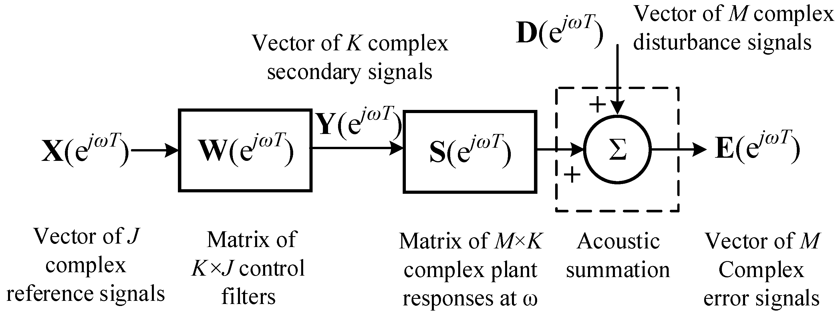
The block diagram of the multichannel ANC (MCANC) system is shown in Figure 1. Acoustic summation of the disturbance signals and secondary source signals (at the error microphone locations) yields a complex vector of residual signals that can be represented in steady-state by
where the normalized frequency will henceforth be omitted for brevity. J reference microphones are configured with K secondary sources, where a vector of reference signals , are filtered by a corresponding set of control filters to yield a vector of secondary source output signals (i.e.,). The contribution of the K secondary sources at the M error microphone locations is , where is the secondary path transfer function at frequency .
2.1. Separating the Active Noise Control Problem
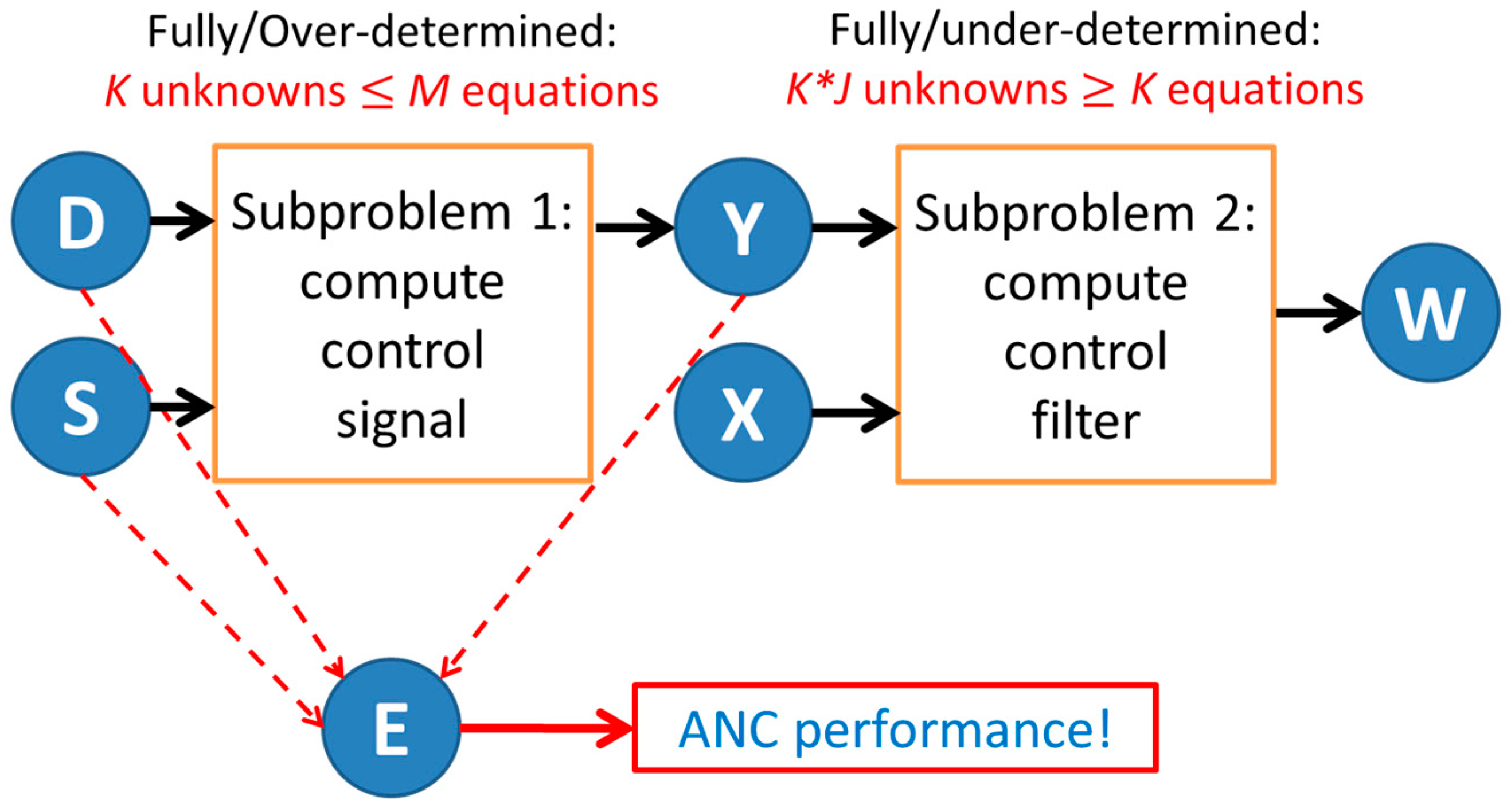
The aim of ANC is to obtain optimal control filters that yield the optimum performance based on certain objective functions [22]. Before deriving the optimal solution for the control filters, we delve into the formation of the multichannel ANC problem. As shown in Figure 2, the ANC problem can be readily divided into 2 subproblems. In the subproblem 1, our aim is to obtain the optimal secondary outputs from input signals and secondary paths so that the cost function can be optimized. In the subproblem 2, based on optimal secondary outputs and reference signals , we derive the optimal control filters . It is intuitive that the performance of the ANC system is only directly related to secondary outputs, whereas the control filters do not contribute directly as long as desired secondary output can be obtained with the control filters. This separation helps to simplify the multichannel ANC problem as follows.
According to [22], a multichannel ANC system usually has more or at least an equal number of error microphones (or control points) as compared to the secondary sources, i.e., casting problem 1 into either an overdetermined or fully-determined problem. In this case, we can define the cost function as the sum (or using a weighted sum [23]) of the squared error signals:
where superscript is the Hermitian operator. The optimal secondary output can thus be calculated by equating the derivative of (2) to zero, which is expressed as
If we are to add a constraint to limit the secondary output power, the objective function becomes where is the regularization parameter [22]. In this case, we can obtain a more generalized solution for the regularized optimization problem as Using (3), we can further compute the optimal residue error energy as
2.2. The Underdetermined Subproblem 2 and Possible Solutions
After we obtain the optimal secondary outputs , we can solve the subproblem 2 to get optimal solutions for control filters W. In this case, we have the following equation,
Given K equations with K*J unknowns in W, this is obviously an underdetermined problem (for J > 1), which means that there are no unique solutions. The conventional solution employing pseudoinverse of X yields [22]
where This solution, though valid, is not the only solution and it assumes an implicit constraint. With reference to the pseudoinverse in underdetermined systems, the additional constraint in solution (6) is such that the l2-norm power of is minimized, which can be proven using the Lagrange multiplier.
To find alternative solutions to the underdetermined situation in the subproblem 2, other constraints can be introduced. One of the methods is to reduce the number of unknown elements in . This can be achieved by, for example, letting J = 1, which is the case for one single reference microphone. Another alternative method to reduce the number of unknowns in is to consider a so-called colocated method, where we assume the reference microphones are located extremely close to the positions of each secondary source (and also assume their quantities are equal, i.e., J = K). This method was adopted in Murao and Nishimura’s active acoustic shielding (AAS) system to tackle noise from open windows [11]. In this case, we have
where represents element-wise division and the non-diagonal elements in W are zero-valued.
It can be found in the literature [1,22] that the pseudoinverse solution of the optimal control filter in (6) can be realized using the fully-coupled multichannel FxLMS adaptive filtering algorithm. Similar to [24], we can express the control filter update in the frequency domain as
where n is the iteration index, is the step size, and is the updated complex error spectra. Further derivation of (8) leads us to the steady-state control filter
with the convergence condition as , where is the maximum eigenvalue of . Comparing with the optimal pseudoinverse solution given in (6), we verify that the fully-coupled multichannel FxLMS converges to the pseudoinverse solution.
Similarly, we can derive the adaptive filter using the colocation method, where we only consider the diagonal elements in the square matrix (i.e., J = K) W, and assume the rest to be 0. We represent such a diagonalized matrix as and introduce a reference signal matrix as
Thus, we can express the control filter update as
With further derivation, we can obtain the steady-state control filter as
where the convergence condition is , where is the maximum eigenvalue of . Compared to the convergence condition in the fully-coupled multichannel FxLMS, we find that, generally, the convergence condition in the colocated method will have a lower bound because the maximum eigenvalue will likely be greater than the maximum eigenvalue . Comparing with the optimal solution given in (7), we can verify that the colocation-based FxLMS converges to its optimal solution. Following the above derivation, we can derive the secondary source output as
These results suggest that with the colocated method, we could achieve identical secondary source output and hence equivalent noise reduction performance as the fully-coupled multichannel FxLMS method. More importantly, the colocated method simplifies the computational complexity of the ANC system by a factor of K times.
A simulation is conducted to illustrate the findings above. Noise reduction (NR) performance for different tonal noises from 20 Hz to 2000 Hz is computed using
Time-domain free-field simulation of a 2-2-4 overdetermined system (for problem 1) with 2 reference microphones, 2 secondary sources, and 4 error microphones is considered using a setup illustrated in Figure 3a, which is similar to that in [14]. The horizontal distance from the primary source to the reference microphones, secondary sources, and error microphones are 0.2 m, 0.1 m, and 0.2 m, respectively. The spacing between the two reference microphones and secondary sources is 0.2 m, whereas the four error microphones are spaced at 0.1 m, 0.2 m, and 0.1 m. The primary noise signal is captured by the reference microphones as , and by the error microphones as . The secondary sources are generated by filtering the reference microphone signals using the adaptive filters based on the above two FxLMS algorithms, which then go through the secondary paths and are summed with the primary noise at the error microphones, resulting in the error microphone signals . The noise reduction performance (after convergence) of the above two adaptive FxLMS algorithms is shown in Figure 3b. The results reveal that the noise reduction performance of both the fully-coupled based on the adaptation equation (8) and the colocated method based on the adaptation Equation (11) are identical with the theoretical performance, verifying the analyses above, in particular, Equations (3) and (13).
3. Optimal Multichannel ANC for Multiple Noise Scenarios
In practice, the characteristics of the noise in open window scenarios could change over time. The optimal filter that is derived from one condition usually performs poorly in other conditions. Whereas adaptive filters can be employed to update the control filters in real-time to track the changes, the requirement of the error microphones raises privacy concerns, increases computation cost, and manifests as a physical obstruction in a domestic environment. Hence, the goal here is to design an optimal fixed filter method that could potentially handle multiple noise scenarios. In the ANC through open windows, the traffic noise arriving at the opening from nearby roads tends to exhibit a plane wave characteristic [25,26]. In the consideration of traffic noise impinging at different floors of a high-rise building, the angles of noise incidence are fixated at each floor [10]. When more urban noise sources, such as from trains and/or aircraft, are considered, noise impinging at the window aperture becomes more complex.
3.1. Optimal Control for Multiple Incidences
Let be the ith incidence angle of the impinging noise. First, we obtain the optimal secondary outputs using (3). Clearly, our aim here is to obtain a single control filter W that can always yield optimal secondary outputs, which is given by
Revisiting the subproblem 2 in Figure 2, we know that for each incident angle, (15) is underdetermined. Therefore, we may cast more constraints, which in this case, means different incident angles. Consider J reference microphones and K secondary sources, we have J*K unknown elements in W. Therefore, we could combine J equations of (15) with different incident angles, and arrive at
where , and . Equation (16) yields a fully-determined system, where one unique solution can be obtained by
We will henceforth refer to this method as the full-rank optimal fixed filter.
Furthermore, considering that in a practical scenario, the direction of noise could vary from −90° to 90°, a full-rank optimal filter could only cover J incidences, resulting in a degraded performance in those directions that are not selected. With this consideration, we can extend the full-rank factorization into an overdetermined factorization, where directions are considered. Similar to (16), the overdetermined optimal filter can be derived as
where , and . It is not difficult to understand that the overdetermined optimal filter could yield a more balanced noise reduction performance than the full-rank optimal filter in broader incidence angles, at the cost of sacrificing performance in the angles selected in the full-rank method.
3.2. Optimal Control for Stochastic Disturbances
In the above sections, we discussed optimal control for deterministic signals. In this section, we consider a general case with stochastic disturbances, i.e., D and X becomes non-stationary. In this case, we can rewrite (3) as
where n is the time index. Correspondingly, the optimal control filter W shall also change from time to time to achieve the optimal performance. In the case where only a fixed filter is realizable, we could factorize all available time frames (say N frames) into the calculation of a fixed optimal filter, and obtain
where , and . Combining (19) and (20), we can obtain the final solution for a fixed optimal filter in the time-varying case as
where . For large N, we can express the cross-spectral density matrix and spectral density matrix and express (21) as
which is consistent with [22]. In a practical case, the statistical analysis of the spectral pattern of the noise will be useful in implementing the fixed optimal control filter. The stochastic optimal control solution, though having been well established in the literature, did reveal that the proposed MCANC framework with underdetermined system brings insights into ANC solutions. However, a full evaluation of this method, as it is beyond the scope of this paper, will not be reported in the following sections.
4. Numerical Experiment Results and Discussions
The finite element method (FEM) computation plane, as depicted in Figure 4, is a 2D representation of a rectangular aperture (i.e., open window) in a rigid thin wall. Eight secondary sources are placed 0.125 m apart within the 1-m wide window to control the incident plane waves entering the window at angle , according to the guidelines in [27]. The entire computation plane is enclosed by a perfectly-matched layer so that all waves are damped to simulate a free-field condition. The acoustic power radiation from the window due to the noise can be calculated based on the far-field formulation as [21]
where r is the radius of the far-field evaluation arc, is the density of air, and c is the speed of sound in air. The acoustic power radiation after ANC can be expressed as
Finally, the acoustic power attenuation (i.e., noise reduction NR) can be calculated as
In this simulation, we evaluate the acoustic power radiated through the aperture by minimizing the sum-of-the-squared error at 1100 points in the far-field arc with a radius r = 10 m. Hence, the 1100 evaluation points in the optimal control formulation is analogous to the error microphones in a physical adaptive ANC system. In this scenario, the ‘error microphones’ are arranged such that the total sound power radiating from the aperture is minimized, which results in global control in the entire room interior. The optimal secondary source output is calculated based on (3), where the secondary paths are determined from FEM simulation. This is similar to the process as detailed in [28]. The ‘reference’ signals are retrieved from the FEM simulations at the position of the secondary sources depicted by qn in Figure 4. This arrangement replicates a collocated reference microphone and secondary source. Incidence angles of the plane waves are considered from −90° (noise from the top) to 90° (noise from the bottom) at an interval of 1°.
4.1. Performance of the Full-Rank Optimal Filter
Based on the optimal secondary source output computed from (3), we can obtain the theoretical optimal noise reduction performance for the setup specified in Figure 4. The noise reduction at five angles of incidence with frequencies from 0 to 2000 Hz is illustrated in Figure 5. Noise reduction performance reduces as frequency increases, as dictated by the control source separation distances and its relative position in the aperture [27,29]. The result presented in Figure 5 is consistent with the upper frequency limit of control defined in [27] as . The attenuation performance is identical for all incidence angles at low frequencies but deteriorates rapidly as they approach their upper frequency limits of control.
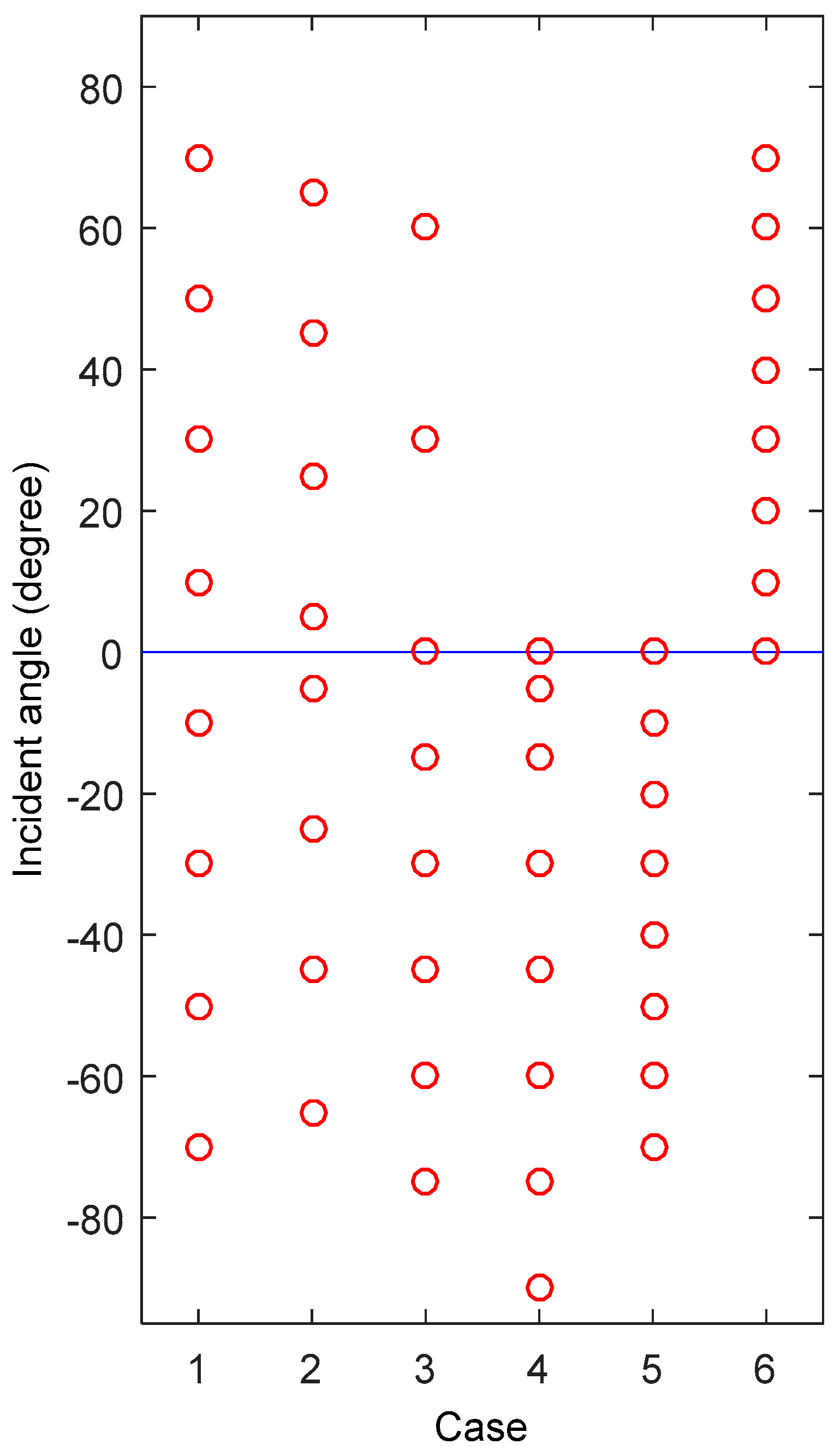
Next, we construct the full-rank optimal filter in the same setup. Since the number of secondary sources is K = 8, we can include eight incidence angles in (16) to obtain the full-rank optimal filter W. Six sets of the eight incidence angles are listed in Table 1 and illustrated in Figure 6. We calculate the full-rank optimal filter using all eight incidences in each case and compute its noise reduction performance. These results are illustrated in Figure 7, Figure 8, Figure 9, Figure 10 and Figure 11.
In Figure 7, we compare the full-rank optimal filter #1 with the exact optimal filter obtained for each incidence individually. The full-rank filter could only achieve identical performance for those angles selected in the full-rank factorization, except for lower frequencies (e.g., f = 100, 200 Hz), where the noise reduction is significantly large, indicating that the residue noise pressure is close to zero and might be affected by the numerical precision of the simulation. For incidence angles other than the eight incidences used in formulating the filter, the noise reduction performance is degraded. The degradation increases in severity when the incidence angles are farther away from the selected angles, especially for higher frequencies.
To examine the effect of the different sets of the eight incidence angles, we illustrate the performance of the four cases (#1, #2, #3, #4 from Table 1) in Figure 8. Since these cases employ different angles, their performance varies significantly. By visual inspection, it is clear that when more incidences from the negative region are used in the formulation (from case 1 to case 4), better attenuation is observed in the negative incidences than the positive directions. One extreme case is case 4, where all eight selected directions are in the zero and negative region, which yields good attenuation for all negative incidences in general but significantly degrades for positive incidences.
In Figure 9, we further compare two such selections that only cover the negative directions, i.e., case 4 and case 5 in Table 1. The key difference between these two cases is that case 5 ignores the extreme directions from −90° to −70° and hence occupies more directions in −70°to 0° range. This selection is motivated by the observation that at extreme incidence angles, the noise that enters the window are at lower levels than higher incidences. Overall, results in Figure 9 indicate that with the selection in case 5, we can achieve optimal performance for almost all negative directions.
Figure 10 illustrates the noise reduction performance for the full-rank optimal filters with formulation cases 5 and 6, where only negative and positive directions are covered, respectively. The interval of 10° is used in both cases. A distinct symmetrical performance is observed where each optimal filter performs optimally in its respective half of the entire incidence range. This result implies that if the ANC system permits, two full-rank optimal filters can be applied to cover all angles of noise incidence. Note that a priori information of the approximate noise incidence (positive or negative) is required for switching the filters.
4.2. Performance of the Overdetermined Optimal Filter for Single Noise Incidence
In the previous subsection, we evaluate the performance of the full-rank optimal filters and found that in the range of incidence angles from −90° to 90°, no single full-rank filters could achieve identical attenuation performance as the exact optimal filters obtained for each incidence. Therefore, we shall consider the overdetermined optimal filter method, as expressed in (18). In Figure 11, we compare the full-rank optimal filter case 1 with the overdetermined optimal filter that selects all 181 incidences from −90° to 90° at 1° interval (termed as “case 1”). Although the overdetermined optimal method does not outperform the full-rank filter at all incidences, its attenuation performance is, on average, superior across the entire range of incidences, especially at higher frequencies. Furthermore, we investigate the influence on the attenuation performance with respect to the number of incidences used in the overdetermined factorization. On this note, we consider three overdetermined formulations, which employs (i) 181 incidences at 1° interval, (ii) 19 incidences at 10° interval, and (iii) 10 incidences at 20° interval. Based on the results in Figure 12, we can observe that the performance of the overdetermined optimal filter case 2 with 19 incidences resembles the case 1 with 181 incidences, whereas the case 3 with 10 incidences yielded inferior overall performance. Thus, we can compute the overdetermined optimal filter with only 19 incidences at 10° interval.
4.3. Performance of Optimal Filters for Two Noise Incidences
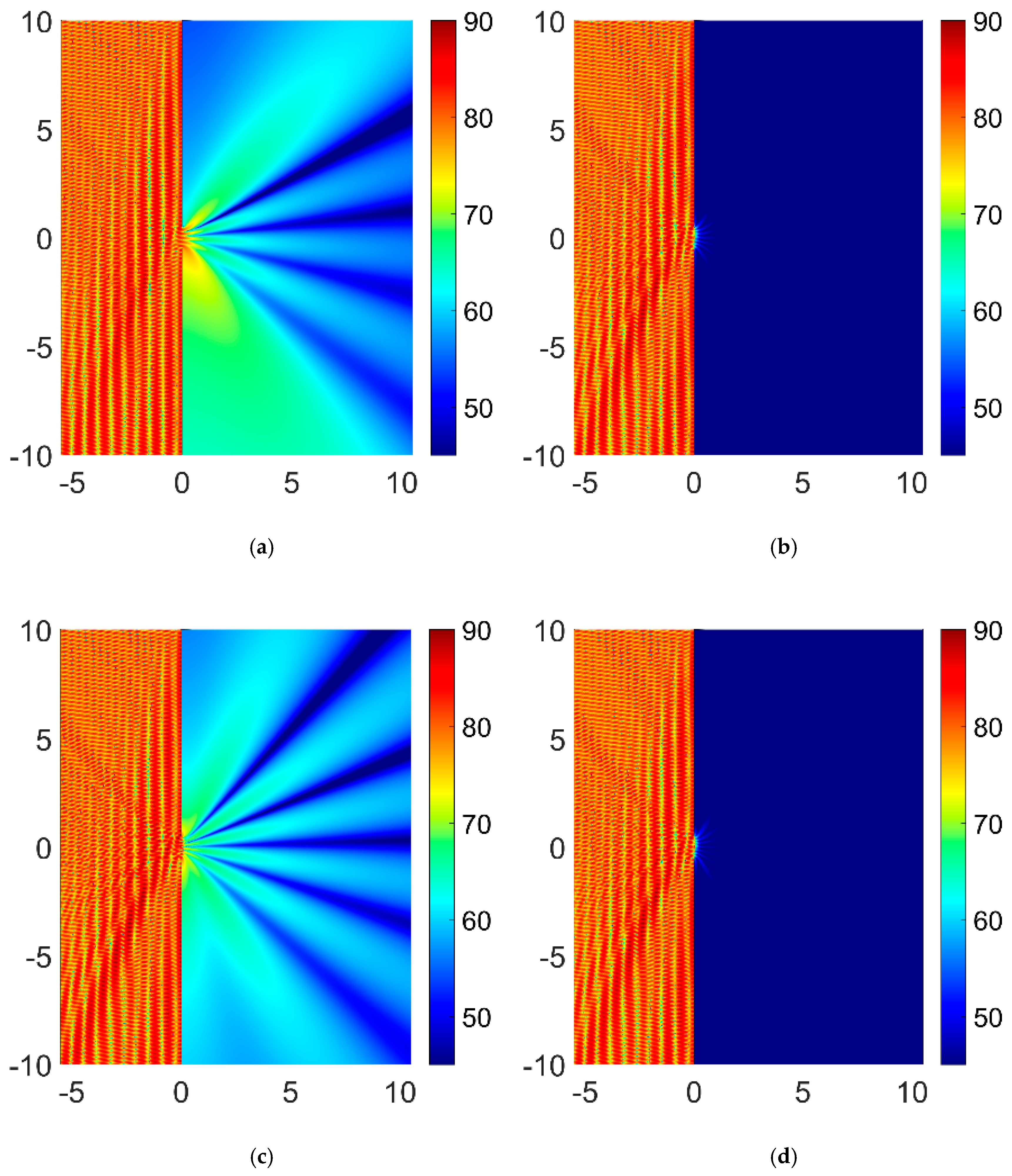
In practical cases, the incoming noise could be more complicated. One typical example is that there are multiple noise sources producing plane wave noise from different directions. In this subsection, we evaluate the performance of the optimal filter in the case of two plane waves. The amplitudes of the two plane waves are set to be 2:1, but their directions are randomized. We run the simulation for 20 cases and illustrate the noise reduction performance of the exact, full-rank (case 1), and overdetermined (case 1 with 181 incidences) optimal filters. The full-rank optimal filter suffers from significant performance degradation, whereas the overdetermined optimal filter yields a very close performance compared to the exact optimal filter, as shown in Figure 13. The sound pressure distribution of the 2D sound field in the FEM simulation for two noise sources at 1000 Hz is exemplified in Figure 14, showing that the global control is achieved in both the exact and overdetermined optimal filters, but not in the full-rank method. The overdetermined optimal method has thus far been robust to a single noise source impinging from any incidence and two noise sources simultaneously from random incidence angles, which can be extended to multiple source incidences.
5. Conclusions
In this paper, we revisit the multichannel active noise control problem. By separating this problem into two subproblems, we find that in a general multiple-input–multiple-output setup, the subproblem 2, i.e., obtaining the optimal control filter from reference signals and optimal secondary outputs, is usually underdetermined with more than one solution. The underdetermined system presents an opportunity to simplify the control filter that achieves equivalent performance or even extends the capability of a fixed optimal filter to handle complex scenarios. For example, we may simplify the control filter by only activating the diagonal elements in the control filter matrix, arriving at the so-called colocated control, which yields the exact optimal secondary output and hence achieves the same noise reduction performance as the fully-coupled multichannel system. Similar observations were found in their adaptive realizations.
Furthermore, the underdetermined system is leveraged to develop the full-rank and overdetermined realization by introducing constraints to derive a fixed optimal control filter, which could be employed to handle noise from multiple angles of incidence. The performance of the full-rank and overdetermined optimal control filter is investigated numerically using FEM simulations. The attenuation performance of the full-rank optimal filter is optimal for incidences utilized in its realization but degrades as the noise incidence deviates from those selected directions. Notably, a full-rank method that evenly selects all eight directions from either the entirely positive or negative direction between −90° to 90° could achieve optimal performance in their entire respective incidence ranges. This implies that a single incidence used in the formulation of the filter could yield optimal attenuation to the neighboring incidence within ±5°, and the extreme incidences (near ±90°) are not required to achieve good global attenuation. Therefore, we can employ two full-rank optimal filters to cover the entire 180° range.
In contrast, the overdetermined optimal filter achieves a better average performance across the entire range of incidences with a single filter. The realization of the overdetermined optimal filter does not demand a fine resolution of incidences, where an interval of 10° across the entire range of incidence angles was shown to be sufficient. Finally, we show that the overdetermined optimal filter outperforms the full-rank optimal filter in a more complex noise environment such as with multiple noise sources. Moving forward, it is necessary to understand the feasibility of applying the proposed overdetermined optimal control method in a practical setup. Furthermore, it is interesting to understand how the overdetermined optimal control method compares to the stochastic optimal control method under the various practical use cases with varying noise incidence. The analysis and simulation studies presented in this paper could facilitate the development of the optimal fixed filter for ANC in more dynamic scenarios, not only for multichannel systems, but also for single channel ANC systems such as ANC headphones.
Author Contributions
Conceptualization, J.H. and B.L.; methodology, J.H. and B.L.; software, B.L.; validation, J.H., B.L. and D.S.; formal analysis, J.H.; investigation, J.H. and D.S.; resources, B.L.; data curation, B.L.; writing—original draft preparation, J.H. and B.L.; writing—review and editing, J.H., B.L. D.S. and W.S.G; visualization, J.H. and B.L.; supervision, W.S.G.; project administration, W.S.G.; funding acquisition, W.S.G.
Funding
This material is based on research/work supported by the Singapore Ministry of National Development and National Research Foundation under L2 NIC Award No.: L2NICCFP1-2013-7.
Acknowledgments
The authors wish to thank Steve Elliott of University of Southampton, UK, Masaharu Nishimura of Tottori University, Japan, Tatsuya Murao of Meijo University, Japan, Chuang Shi of University of Electronic Science and Technology of China for the fruitful discussions and constructive comments on this work.
Conflicts of Interest
The authors declare no conflict of interest. The funders had no role in the design of the study; in the collection, analyses, or interpretation of data; in the writing of the manuscript, or in the decision to publish the results.
References
- Kuo, S.M.; Morgan, D.R. Active Noise Control Systems: Algorithms and DSP Implementations; Wiley: Hoboken, NY, USA, 1996. [Google Scholar]
- Kajikawa, Y.; Gan, W.-S.; Kuo, S.M. Recent advances on active noise control: Open issues and innovative applications. APSIPA Trans. Signal Inf. Process. 2012, 1, e3. [Google Scholar] [CrossRef]
- Cheer, J.; Elliott, S.J. Multichannel control systems for the attenuation of interior road noise in vehicles. Mech. Syst. Signal Process. 2015, 60–61, 753–769. [Google Scholar] [CrossRef]
- Samarasinghe, P.N.; Zhang, W.; Abhayapala, T.D. Recent Advances in Active Noise Control Inside Automobile Cabins: Toward quieter cars. IEEE Signal Process. Mag. 2016, 33, 61–73. [Google Scholar] [CrossRef]
- Wang, S.; Tao, J.; Qiu, X. Controlling sound radiation through an opening with secondary loudspeakers along its boundaries. Sci. Rep. 2017, 7, 13385. [Google Scholar] [CrossRef] [PubMed] [Green Version]
- Lam, B.; Shi, C.; Shi, D.; Gan, W.-S. Active control of sound through full-sized open windows. Build. Environ. 2018, 141, 16–27. [Google Scholar] [CrossRef]
- World Health Organization, Regional Office for Europe. Burden of Disease from Environmental Noise: Quantification of Healthy Life Years Lost in Europe; WHO: Copenhagen, Denmark, 2011. [Google Scholar]
- Nugent, C.; Blanes, N.; Fons, J.; de la Maza, M.S.; Ramos, M.J.; Domingues, F.; van Beek, A.; Houthuijs, D. Noise in Europe 2014; Publications Office of the European Union: Luxembourg, Luxenbourg, 2014; ISBN 9789292135058. [Google Scholar]
- World Health Organization, Regional Office for Europe. Environmental Noise Guidelines for the European Region; The Regional Office for Europe of the WHO: Copenhagen, Denmark, 2018; ISBN 978 92 890 5356 3. [Google Scholar]
- Lam, B.; Gan, W.-S. Active Acoustic Windows: Towards a Quieter Home. IEEE Potentials 2016, 35, 11–18. [Google Scholar]
- Murao, T.; Nishimura, M. Basic Study on Active Acoustic Shielding. J. Environ. Eng. 2012, 7, 76–91. [Google Scholar] [CrossRef]
- Kwon, B.; Park, Y. Interior noise control with an active window system. Appl. Acoust. 2013, 74, 647–652. [Google Scholar] [CrossRef]
- Fasciani, S.; He, J.; Lam, B.; Murao, T.; Gan, W.-S. Comparative study of cone-shaped versus flat-panel speakers for active noise control of multi-tonal signals in open windows. In Proceedings of the INTER-NOISE and NOISE-CON Congress and Conference, San Francisco, CA, USA, 9–12 August 2015; pp. 1109–1120. [Google Scholar]
- He, J.; Lam, B.; Murao, T.; Ranjan, R.; Gan, W.-S. Symmetric design of multiple-channel active noise control systems for open windows. In Proceedings of the INTER-NOISE and NOISE-CON Congress and Conference, Hamburg, Germany, 21–24 August 2016; pp. 613–622. [Google Scholar]
- Murao, T.; Nishimura, M.; He, J.; Lam, B.; Ranjan, R.; Shi, C.; Gan, W.-S. Feasibility study on decentralized control system for active acoustic shielding. In Proceedings of the INTER-NOISE and NOISE-CON Congress and Conference, Hamburg, Germany, 21–24 August 2016; pp. 1106–1115. [Google Scholar]
- Ranjan, R.; He, J.; Murao, T.; Lam, B.; Gan, W.-S. Selective Active Noise Control System for Open Windows using Sound Classification. In Proceedings of the INTER-NOISE and NOISE-CON Congress and Conference, Hamburg, Germany, 21–24 August 2016; pp. 482–492. [Google Scholar]
- Lam, B.; He, J.; Murao, T.; Shi, C.; Gan, W.-S.; Elliott, S.J. Feasibility of the full-rank fixed-filter approach in the active control of noise through open windows. In Proceedings of the INTER-NOISE and NOISE-CON Congress and Conference, Hamburg, Germany, 21–24 August 2016; pp. 3548–3555. [Google Scholar]
- Huang, H.; Qiu, X.; Kang, J. Active noise attenuation in ventilation windows. J. Acoust. Soc. Am. 2011, 130, 176–188. [Google Scholar] [CrossRef] [PubMed]
- Pàmies, T.; Romeu, J.; Genescà, M.; Arcos, R. Active control of aircraft fly-over sound transmission through an open window. Appl. Acoust. 2014, 84, 116–121. [Google Scholar] [CrossRef]
- Carme, C.; Schevin, O.; Romerowski, C.; Clavard, J. Active Noise Control Applied to Open Windows. In Proceedings of the INTER-NOISE NOISE-CON Congres and Conference, Hamburg, Germany, 21–24 August 2016; pp. 3058–3064. [Google Scholar]
- Nelson, P.A.; Elliott, S.J. Active Control of Sound; Academic Press: Cambridge, MA, USA, 1992; ISBN 9780125154260. [Google Scholar]
- Elliott, S.J. Signal Processing for Active Control; Academic Press: London, UK, 2001; ISBN 9780122370854. [Google Scholar]
- Elliott, S.J.; Cheer, J. Modeling local active sound control with remote sensors in spatially random pressure fields. J. Acoust. Soc. Am. 2015, 137, 1936–1946. [Google Scholar] [CrossRef] [PubMed]
- Elliott, S.J.; Boucher, C.C. Interaction between multiple feedforward active control systems. IEEE Trans. Speech Audio Process. 1994, 2, 521–530. [Google Scholar] [CrossRef]
- Crocker, M.J. Handbook of Noise and Vibration Control; John Wiley & Sons: Hoboken, NJ, USA, 2007; ISBN 9780471395997. [Google Scholar]
- Murphy, E.; King, E.A. Environmental Noise Pollution; Elsevier: Amsterdam, The Netherlands, 2014; ISBN 9780124115958. [Google Scholar]
- Lam, B.; Elliott, S.; Cheer, J.; Gan, W.-S. Physical limits on the performance of active noise control through open windows. Appl. Acoust. 2018, 137, 9–17. [Google Scholar] [CrossRef]
- Lam, B.; Elliott, S.J.; Cheer, J.; Gan, W.-S. The Physical Limits of Active Noise Control of Open Windows. In Proceedings of the 12th Western Pacific Acoustics Conference, Singapore, Singapore, 6–10 December 2015; Lim, K.M., Ed.; pp. 184–189. [Google Scholar]
- Elliott, S.J.; Cheer, J.; Lam, B.; Shi, C.; Gan, W. A wavenumber approach to analysing the active control of plane waves with arrays of secondary sources. J. Sound Vib. 2018, 419, 405–419. [Google Scholar] [CrossRef]
Figure 1.
Block diagram of the multichannel active noise control system.

Figure 2.
A separation of the multichannel ANC problem into 2 subproblems.

Figure 3.
(a) Setup of a 2-2-4 ANC system and (b) noise reduction performance using the fully-coupled multichannel FxLMS, the colocated FxLMS, and the theoretical optimal performance.
Figure 3.
(a) Setup of a 2-2-4 ANC system and (b) noise reduction performance using the fully-coupled multichannel FxLMS, the colocated FxLMS, and the theoretical optimal performance.
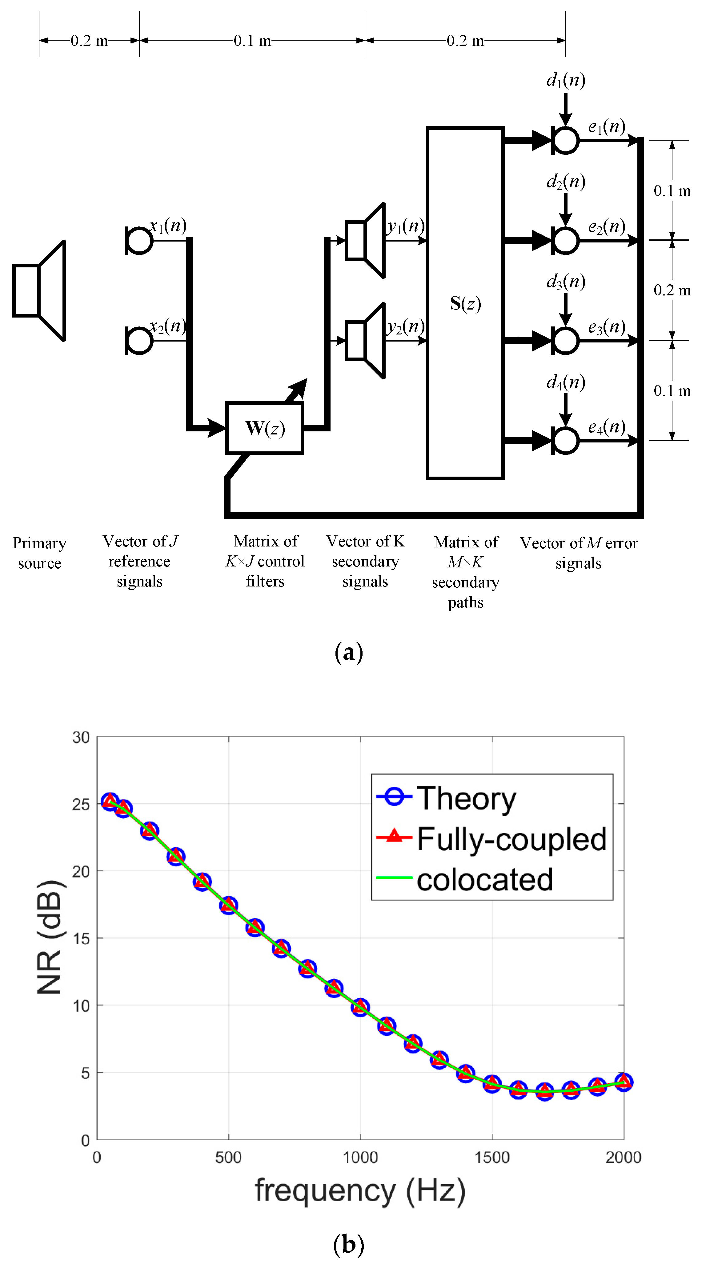
Figure 4.
Finite element method simulation plane.
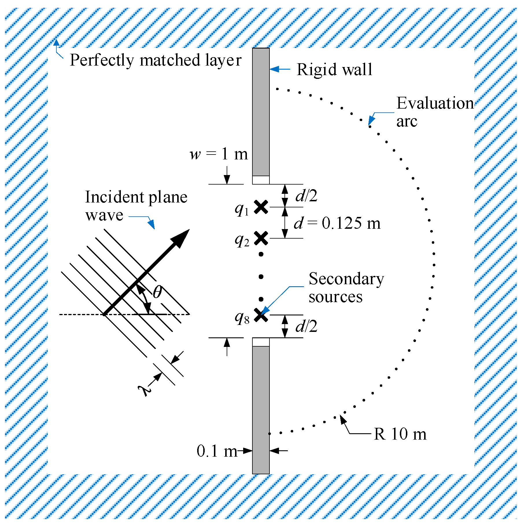
Figure 5.
Noise reduction performance of optimal fixed filter obtained individually.
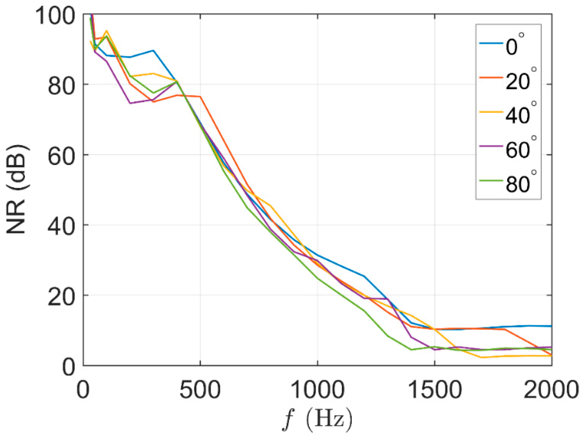
Figure 6.
Illustration of the eight directions selected in the six cases of the full-rank optimal filter.
Figure 6.
Illustration of the eight directions selected in the six cases of the full-rank optimal filter.

Figure 7.
Noise reduction performance of the exact optimal filter and the full-rank optimal filter with case 1 formulations at all incidences from −90° to 90°. The eight incidences are illustrated as markers in a straight line on the bottom to aid the interpretation (this also applied to following figures).

Figure 8.
Noise reduction performance of four cases of the full-rank optimal filters, at frequency (a) 400 Hz, (b) 1000 Hz.
Figure 8.
Noise reduction performance of four cases of the full-rank optimal filters, at frequency (a) 400 Hz, (b) 1000 Hz.
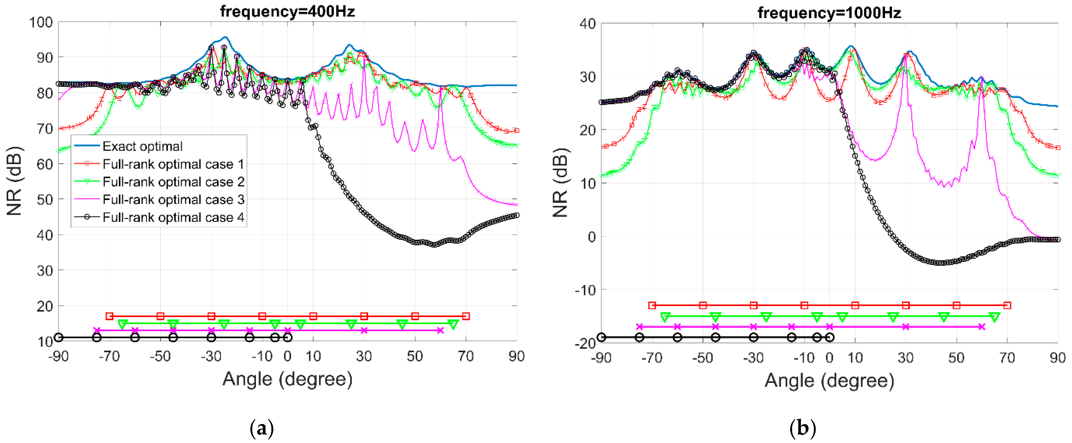
Figure 9.
Noise reduction performance of two cases of the full-rank optimal filters that only consider the negative directions, at frequency (a) 400 Hz, (b) 1000 Hz.
Figure 9.
Noise reduction performance of two cases of the full-rank optimal filters that only consider the negative directions, at frequency (a) 400 Hz, (b) 1000 Hz.

Figure 10.
Noise reduction performance of two cases of the full-rank optimal filters that only consider the negative and positive directions, respectively, at frequency (a) 400 Hz, (b) 1000 Hz.
Figure 10.
Noise reduction performance of two cases of the full-rank optimal filters that only consider the negative and positive directions, respectively, at frequency (a) 400 Hz, (b) 1000 Hz.
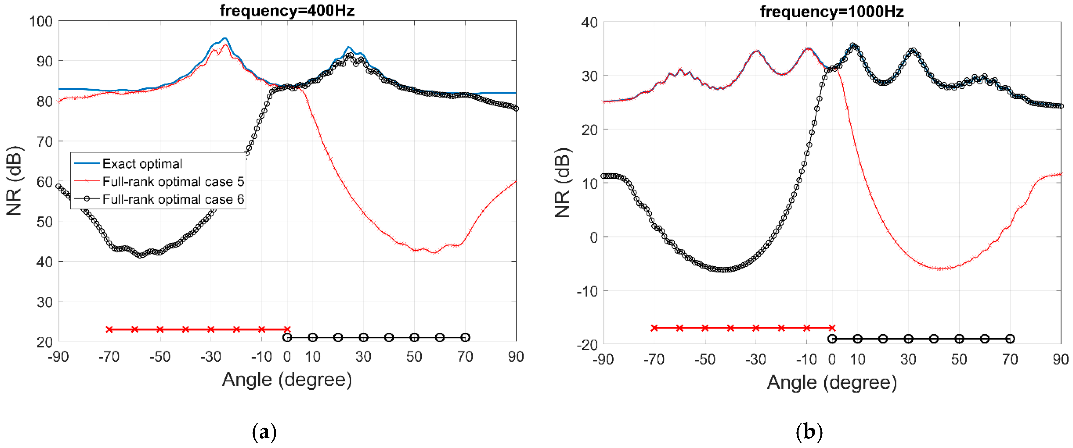
Figure 11.
Noise reduction performance of full-rank optimal filter case 1 and overdetermined optimal filter case 1, at frequency (a) 400 Hz, (b) 1000 Hz.
Figure 11.
Noise reduction performance of full-rank optimal filter case 1 and overdetermined optimal filter case 1, at frequency (a) 400 Hz, (b) 1000 Hz.

Figure 12.
Noise reduction performance of three overdetermined optimal filter cases, at frequency (a) 400 Hz, (b) 1000 Hz.
Figure 12.
Noise reduction performance of three overdetermined optimal filter cases, at frequency (a) 400 Hz, (b) 1000 Hz.
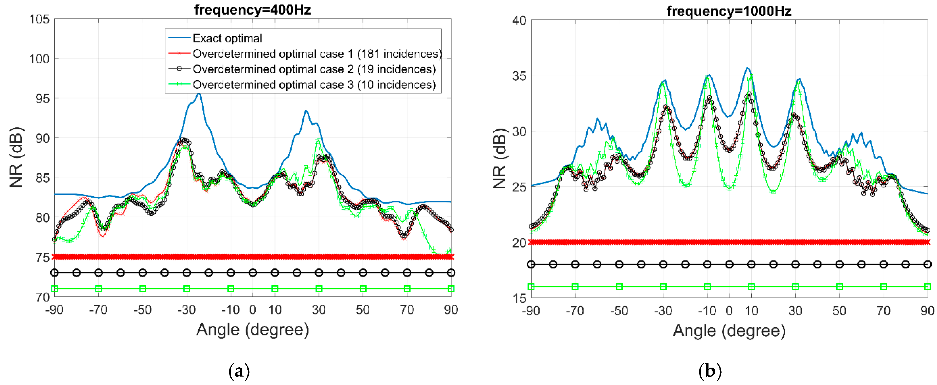
Figure 13.
Noise reduction performance of the full-rank optimal filter and the overdetermined optimal filter for plane wave noise from two directions, at frequency (a) 400 Hz, (b) 1000 Hz.
Figure 13.
Noise reduction performance of the full-rank optimal filter and the overdetermined optimal filter for plane wave noise from two directions, at frequency (a) 400 Hz, (b) 1000 Hz.
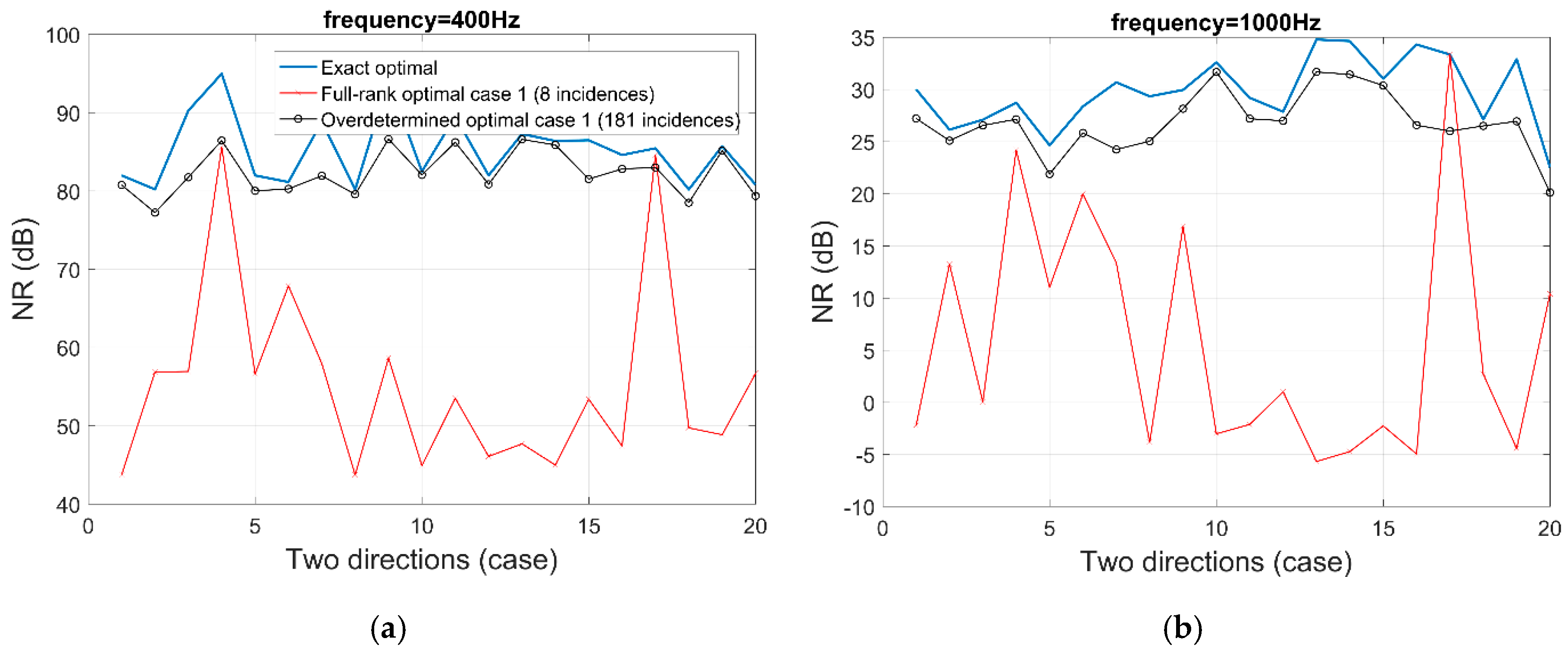
Figure 14.
2D sound pressure level (dB) of (a) primary noise only, (b) exact optimal control, (c) full-rank optimal control (case 1), and (d) overdetermined optimal control (case 1 with 181 incidences) for two noise sources at 1000 Hz. The units of the axes are meters.
Figure 14.
2D sound pressure level (dB) of (a) primary noise only, (b) exact optimal control, (c) full-rank optimal control (case 1), and (d) overdetermined optimal control (case 1 with 181 incidences) for two noise sources at 1000 Hz. The units of the axes are meters.

Table 1.
Six cases of eight angles selected in full-rank optimal filter.
| Case/Angle. | 1 | 2 | 3 | 4 | 5 | 6 | 7 | 8 |
|---|---|---|---|---|---|---|---|---|
| #1 | −70 | −50 | −30 | −10 | 10 | 30 | 50 | 70 |
| #2 | −65 | −45 | −25 | −5 | 5 | 25 | 45 | 65 |
| #3 | −75 | −60 | −45 | −30 | −15 | 0 | 30 | 60 |
| #4 | −90 | −75 | −60 | −45 | −30 | −15 | −5 | 0 |
| #5 | −70 | −60 | −50 | −40 | −30 | −20 | −10 | 0 |
| #6 | 70 | 60 | 50 | 40 | 30 | 20 | 10 | 0 |
© 2019 by the authors. Licensee MDPI, Basel, Switzerland. This article is an open access article distributed under the terms and conditions of the Creative Commons Attribution (CC BY) license (http://creativecommons.org/licenses/by/4.0/).
Share and Cite
MDPI and ACS Style
He, J.; Lam, B.; Shi, D.; Gan, W.S. Exploiting the Underdetermined System in Multichannel Active Noise Control for Open Windows. Appl. Sci. 2019, 9, 390. https://doi.org/10.3390/app9030390
AMA Style
He J, Lam B, Shi D, Gan WS. Exploiting the Underdetermined System in Multichannel Active Noise Control for Open Windows. Applied Sciences. 2019; 9(3):390. https://doi.org/10.3390/app9030390
Chicago/Turabian StyleHe, Jianjun, Bhan Lam, Dongyuan Shi, and Woon Seng Gan. 2019. "Exploiting the Underdetermined System in Multichannel Active Noise Control for Open Windows" Applied Sciences 9, no. 3: 390. https://doi.org/10.3390/app9030390
Note that from the first issue of 2016, this journal uses article numbers instead of page numbers. See further details here.