Some Applications of ANN to Solar Radiation Estimation and Forecasting for Energy Applications

Abstract

In solar energy, the knowledge of solar radiation is very important for the integration of energy systems in building or electrical networks. Global horizontal irradiation (GHI) data are rarely measured over the world, thus an artificial neural network (ANN) model was built to calculate this data from more available ones. For the estimation of 5-min GHI, the normalized root mean square error (nRMSE) of the 6-inputs model is 19.35%. As solar collectors are often tilted, a second ANN model was developed to transform GHI into global tilted irradiation (GTI), a difficult task due to the anisotropy of scattering phenomena in the atmosphere. The GTI calculation from GHI was realized with an nRMSE around 8% for the optimal configuration. These two models estimate solar data at time, t, from other data measured at the same time, t. For an optimal management of energy, the development of forecasting tools is crucial because it allows anticipation of the production/consumption balance; thus, ANN models were developed to forecast hourly direct normal (DNI) and GHI irradiations for a time horizon from one hour (h+1) to six hours (h+6). The forecasting of hourly solar irradiation from h+1 to h+6 using ANN was realized with an nRMSE from 22.57% for h+1 to 34.85% for h+6 for GHI and from 38.23% for h+1 to 61.88% for h+6 for DNI.

1. Introduction

Solar thermal or electrical systems require high quality solar radiation measurement instruments in order to accurately measure solar energy received on the plant. Poor quality data or too short data series can generate errors in plant design, performance, and production forecasting, negatively impacting return on investment.

Unfortunately, measures of solar radiation are sparse and inaccurate over the world; there are still large areas without any solar radiation observations [1]. Investments and maintenance costs for each measurement site are not negligible and even in industrialized countries, the national network often consists in a relatively small number of solar radiation stations [2]; and the measurement quality varies from a network to another, often by lack of maintenance and calibration. The measuring devices’ price is an important part of the process cost of collecting solar data, especially for non-profit institutions, such as schools or universities [2].

The amount of meteorological stations measuring solar irradiance through the world is difficult to count because various sources give different information [3]. Even so, only 1000 continental stations around the world are measuring solar radiation [4].

In these conditions, it is interesting to look for some relations between sparse solar radiation data and more measured meteorological data as temperature, humidity, and wind speed. Satellite observations are used for determining the solar irradiation on the ground, with a good accuracy, but the time step of the estimated data is relatively large (minimum hourly).

A bibliographical study showed [5] that artificial neural networks (ANN) were developed between meteorological parameters and solar irradiations, but generally only for averaged values of solar irradiations (on a monthly or annual basis); today, data with a short time granularity (minute, 5-min) must be known for interesting applications in solar energy. In the first part of this paper, 10 meteorological inputs (measured or calculated) are available and then 2¹⁰ − 1 = 1023 combinations of input data are possible, from 10 ANN with only one input to one ANN with 10 inputs. All these combinations are tested and the best configurations are discussed.

The solar panels are rarely fixed horizontally and the global tilted irradiation (GTI) is rarely measured and must be estimated from global horizontal irradiation (GHI), more often available; using pyranometers with various inclinations is costly and their maintenance is constraining. Thus, it is useful to develop accurate methods for determining GTI from only GHI. This objective is difficult to reach with conventional physical relations because the sky anisotropy makes the modeling of the sky diffuse radiation difficult [6,7,8]. ANN methods generally realize the same conversion with an improved adequacy (generally, at an hourly scale), and they outperform [9,10,11,12,13] the traditional methods due to the inherent non-linearity in solar radiation data. In this work, an ANN model is developed and optimized for “tilting” 5-min time step solar data.

The stochastic and intermittent behavior of the solar resources poses numerous problems for the electricity grid operator [5] and limits the future development of the phovoltaic (PV) and concentrated solar power (CSP) plants. To improve the integration of such systems, the solution consists in introducing energy storages and developing smart grids as well as implementing production and consumption forecasting.

The forecasting of the output power of solar energy systems is required for good operation of the power grid and for optimal management of electrical flows [3]. It is essential to estimate the energy reserves, to schedule the power systems, to optimally manage the storage, and to trade in the electricity market [14,15,16]. Thus, predicted and anticipated events are easier to manage. Electricity must be produced by CSP and/or PV plants; the first ones convert the direct normal irradiation (DNI) into heat through focusing receivers and PV ones enable direct conversion of GHI into electricity through semiconductor devices [3,17]. The literature shows that the most efficient methods for a forecast at a short time horizon from one hour (h+1) to six hours (h+6) are time series analysis and artificial intelligence methods [18]. If a large literature exists about the GHI forecasting [3,15,17,18,19], this literature is poorer concerning DNI being more difficult to predict because its variations are deeper and more frequent [20,21]. ANN predictive models are implemented to forecast hourly GHI and DNI from h+1 to h+6.

Section 2 presents the data used in this paper (Bouzareah, Algeria for estimation purposes and Odeillo, France for forecasting purposes), the preprocessing used on this data, and the calculated error metrics to estimate the accuracy of ANN models.

Section 3 gives some information on the ANN implementation for estimation and forecasting.

In Section 4 and Section 5, the main results on the estimation of 5 min-GHI from other meteorological parameters and of the 5 min-GTI from GHI measurements are presented.

Section 6 shows the results of the ANN forecasting of hourly GHI and DNI for a time horizon from h+1 to h+6.

2. Meteorological Stations and Data

2.1. The Meteorological Stations

The two first studies were realized using meteorological data measured in the meteorological station belonging to the Renewable Energies Development Centre (CDER) located in Bouzareah near Algiers (latitude: 36.8° N; longitude: 3.17° E) at an altitude of 347 m. The site is characterized by a Mediterranean climate with dry and hot summers and damp and cool winters. The data were measured each second and stored each 5 min from April 2011 to April 2013 (24 months of 5-min data). The measured data and the calculated astronomical data (horizontal extraterrestrial irradiation (EHI), solar declination, δ, and zenith angle, ${\theta }_z$ [22]), are presented in

Table 1. Available meteorological data in Bouzareah.

Data	Symbol	Unity
Measured data
Global horizontal solar irradiation	GHI	Wh.m−2
Global tilted solar irradiation (36.8°)	GTI	Wh.m−2
Ambient temperature	T	°C
Relative humidity	H	%
Wind speed	WS	m.s−1
Wind direction	WD	degree
Precipitation	Pr	mm
Sunshine duration	S	minutes
Atmospheric pressure	P	mbar
Calculated data
Extraterrestrial Horizontal irradiation	EHI	Wh.m−2
Solar declination	δ	degree
Zenith angle	θz	degree

.

The tilted solar data were measured for a 36.8° tilt angle equal to the latitude of Bouzareah (optimal angle for a maximum annual irradiation). The data basis contains 12 5-min parameters, 9 measured and 3 calculated. Each data was previously verified in order to extract outliers.

The forecasting work was realized from GHI and DNI data provided by the PROMES laboratory (CNRS UPR 8521) located in the south of France in Odeillo (Pyrénées Orientales, France, 42°29 N, 2°01 E, 1550 m asl), the station is located in the mountains, at about 100 km from the Mediterranean sea and presents an often high nebulosity. The solar data are measured and stored with a 1 min time granularity. This meteorological station is in altitude, the climate is very perturbed, the rainfall continues to be present during the driest months, the variability of solar radiation is high, and thus its forecasting is more difficult to realize. Two years of hourly data were available i.e., 17 520 data, for both GHI and DNI.

2.2. Cleaning and Preprocessing

For Bouzareah, each 5-min data were first verified to extract outliers or missing data. Then, the data during which the sun rises or sets were deleted because the mask effect of the environment and the no-reliable response of pyranometers at a high zenith angle (cosine effect) introduced some errors. Thus, over the 2 years, 75674 validated 5-min data were available for each parameter.

For the Odeillo’s data, an automatic quality control used in the frame of the GEOSS project (Group on Earth Observation System of System) [23] was applied. Before introducing the solar data into the machine learning process, the data were cleaned and filtered.

For forecasting purposes, it is common to filter out the data to remove night hours and to conserve them only between sunrise and sunset. As for Bouzareah, the data near sunset and sunrise are sources of errors and a pre-processing operation was applied based on the solar elevation: Solar radiation data for which the solar elevation is lower than 10° were removed [15,24]. Two years of hourly data were used in this study. After cleaning and filtering, the total number of hourly data for each solar component (GHI and DNI) was 10559 (about 60% of the data were not used (2% for outliers’ data and 58% for sun elevation less than 10°)). These solar data were then transformed into stationary data by a method described in Section 6.

2.3. Statistical Index for Accuracy Evaluation

There are no well-defined error metrics standards, which makes the forecasting and estimation methods difficult to compare [25]. A benchmarking exercise was realized within the framework of the European Actions Weather Intelligence for Renewable Energies (WIRE) [26], with the objective to evaluate the state of the art concerning models’ performances for short term renewable energy forecasting. They concluded that: “More work using more test cases, data and models needs to be performed in order to achieve a global overview of all possible situations. Test cases located all over Europe, the US and other relevant countries should be considered, trying to represent most of the possible meteorological conditions”.

In this paper, these five error metrics were used:

-

The mean absolute error (MAE) defined by:

$$MAE=\frac{1}{N}\times {\displaystyle \sum }_{i=1}^N\left|{\widehat{X}}_{t_i}-X_{t_i}\right|$$

(1)

${\widehat{X}}_{t_i}$ being the forecasted outputs (or predicted values), $X_{t_i}$ the observed data, and N the number of observations.

-

The root mean square error (RMSE), more sensitive to important forecast errors, and hence suitable for applications where small errors are more tolerable than larger ones, as in utility applications. It is probably the reliability factor that is the most widely used:

$$RMSE=\sqrt{\frac{1}{N}\times {\displaystyle \sum }_{i=1}^N{\left({\widehat{X}}_{t_i}-X_{t_i}\right)}^2}$$

(2)

-

The mean bias error (MBE), mainly used to estimate the bias of the model:

$$MBE=\frac{1}{N}\times {\displaystyle \sum }_{i=1}^N{\left({\widehat{X}}_{t_i}-X_{t_i}\right)}^{}$$

(3)

These errors were then normalized, and the mean value of irradiation is generally used as the reference:

$$nRMSE=\frac{RMSE}{\overline{X}}$$

(4)

$$nMAE=\frac{MAE}{\overline{X}}$$

(5)

with $\overline{X}$ the average value of X calculated on the N data.

3. ANN Method and Implementation

3.1. General Description of ANN Structure

An ANN [27] is a modelling tool able to find complex relationships between inputs and outputs. It is considered as “intelligent” because it works as a human brain:

-

A neural network acquires knowledge through learning; and

-

a neural network’s knowledge is stored within inter-neuron connection strengths known as synaptic weights.

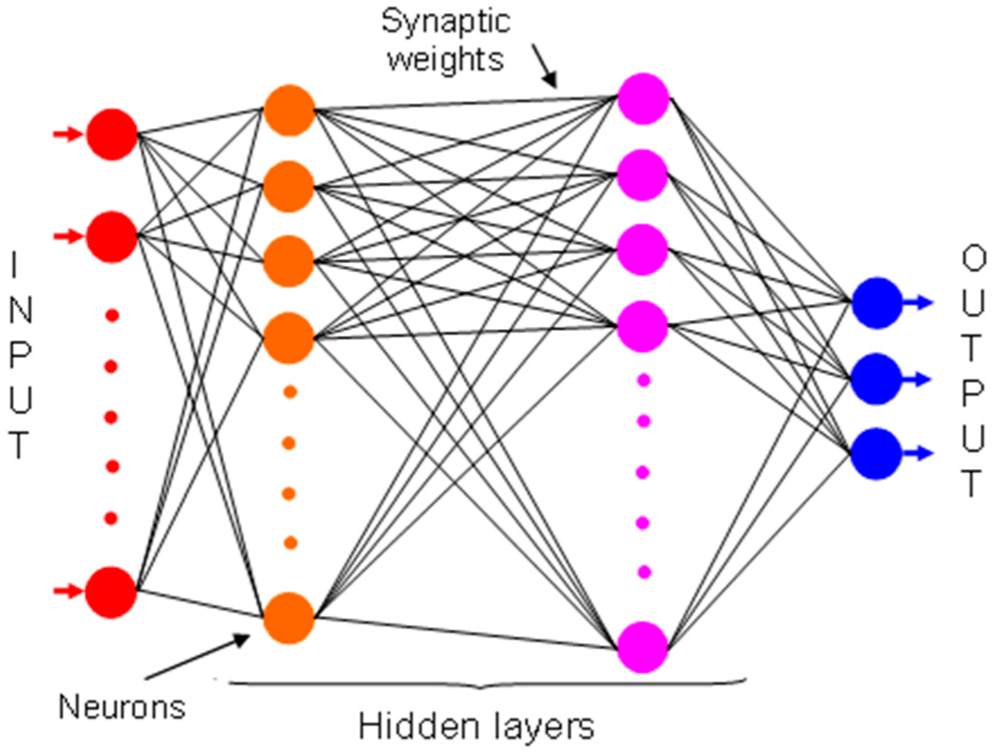
ANNs can represent both linear and non-linear relationships and have their ability to learn these relationships directly from the measured data. Among the various ANN methods, the multilayer perceptron (MLP) using feed-forward back-propagation is often used for empirical estimation in general [28], and in particular [19,29,30], for the estimation of solar radiation. An ANN has a parallel structure with an input layer receiving data, an output layer sending the computed data, and one or several hidden layers lying between the input and output layers as illustrated in Figure 1.

A neuron receives input from other neurons and/or an input data, which represents an external source. In the feed-forward propagation MLP configuration, this connection is unidirectional. Each input, $x_{k,j}$, has an associated weight, $w_{k,j}$ (related to the j-th neuron among p of the k-th layers), which can be modified during the learning phase. The weighted sum, ${{\displaystyle \sum }}_{j=1}^p{w}_{k,j}{x}_{k,j}$, is called the net input to unit j, often written net. The unit computes a function, f, of this weighted sum and is called the activation or transfer function; this function, f, produces an output, O, of a neuron if this sum exceeds a given threshold denoted biases. A bibliographical study conducted to use as activation transfer functions a sigmoid one for the hidden layers and a linear function for the output layer. For the jth neuron of the layer (k+1), O is given by [31]:

$$O=f\left(net\right)=f\left({\displaystyle \sum }_{j=1}^p{w}_{k,j}{x}_{k,j}\right)$$

(6)

This output is then distributed to other neurons as inputs.

3.2. ANN Implementation for GHI and GTI Irradiation

Several steps are applied in view to find the optimized MLP:

-

Choice of the network size (number of hidden layers and hidden nodes per layer): Too small a number of hidden nodes does not allow good learning, but an oversized number increases the training time with a marginal improvement [32,33], need more data and the ANN can be over-trained. In accordance with the principle of parsimony and with the literature [34], only one hidden layer was used.

-

Determination of the optimal number of neurons in the hidden layer: It is realized in testing various configurations and calculating the adequacy. Some empirical rules exist, but their efficiency is not really proven: The number of hidden neurons equal to the inputs number [35], to 75% of it [36], to the square root of the product of the number of inputs and outputs [37]. Here, the number of hidden neurons was taken between 1 and the number of inputs +1. Each MLP architecture was trained 8 times per architecture in order to avoid random effects.

-

Learning (or training) process: It consists in modifying the weights until the gap between the actual and simulated outputs reaches a desired accuracy. The Levenberg–Marquardt learning algorithm (LM) was used as in most studies. Another preprocess called k-fold sampling was used with the dataset [38,39], this cross-validation is a statistical method used to estimate the skill of machine learning models. It is commonly used in applied machine learning to compare and select a model for a given predictive modeling problem, which has a lower bias than other methods [40,41]: It consists in dividing randomly the data set into a training data set (80%) and a test data set (20%), the training set and the test set are different for each fold; this process is repeated k times and the value of the reliability metrics given in this paper are the average value on the k-fold. Here, k is taken equal to 10. Thus, the results are independent of the set of data used for the training; using only one data set (with its own statistical particularities) can reduce the robustness of the conclusions.

Other information specific to each study will be given in the corresponding chapter.

4. Estimation of GHI from Other Meteorological Data

4.1. Method

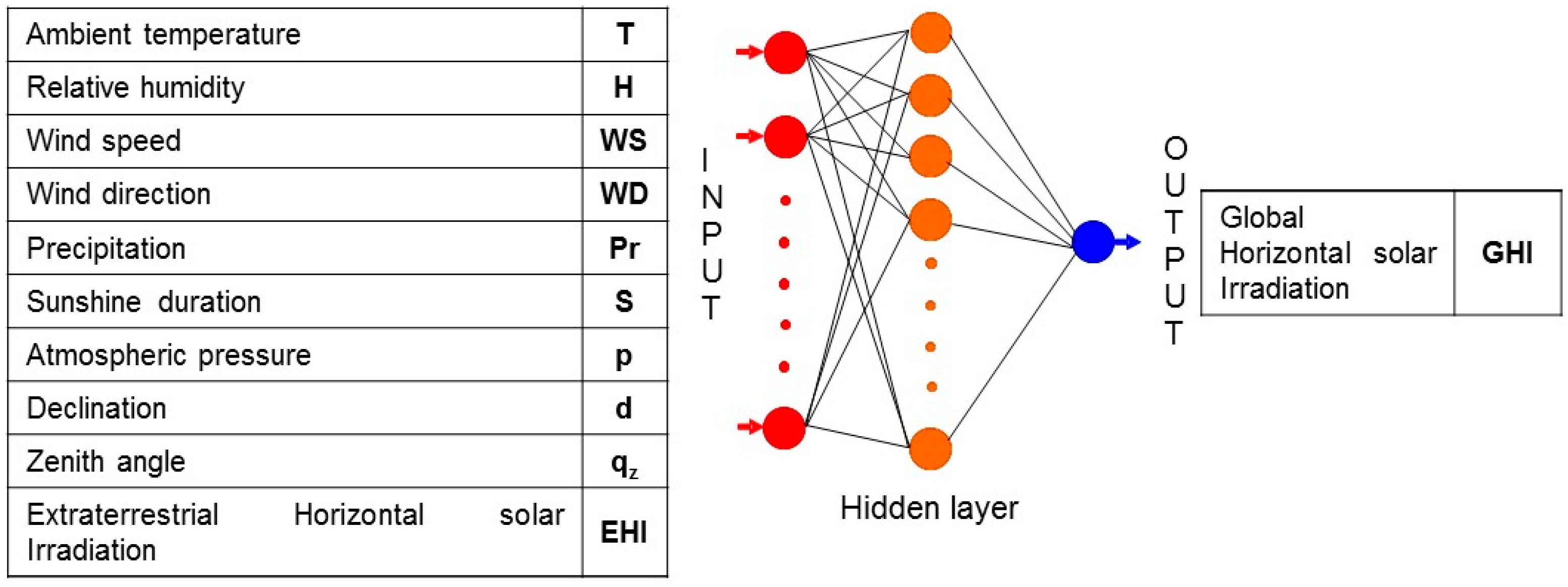
In this study, the data used were measured in Bouzareah (see Section 2.1). Figure 2 shows the ANN structure with all the available inputs.

The sunshine duration is the time expressed in minutes during which the solar irradiance exceeds 120 W/m². It is strongly linked with the solar radiation (Angstrom relation for example).

The number of inputs, 10 (7 measured, 3 calculated), makes the optimization of the MLP structure long and arduous: With 10 inputs, 2¹⁰ − 1 = 1023 combinations of input data are possible.

The choice of the best inputs combination is a prerequisite stage because the parsimony is a basic principle in ANN elaboration, essential for its generalization. Some of the variables bring little information, sometimes no information at all, some of them are redundant, even worse they reduce the model performance. Moreover, an increase of the input number is accompanied by an increase of the hidden neurons and of the calculation time.

The Pearson’s correlation coefficient between each input parameter and the output is determined before using an exhaustive selection (testing 1023 architectures).

4.2. Relationship between Input and Output Data

The Pearson’s correlation coefficient (R) between input variables and GHI and between inputs variables themselves were calculated. When the absolute value of R is near 1, there is a high degree of linear correlation between the two variables; if R = 0, there is no linear correlation, but other relation types can exist.

Computing R between input variables allows an estimation of whether the inputs are redundant and interdependent. The first objective is to rank the statistical linear dependences between the inputs and output; for a large sample of data, the R threshold from which there is a significant link between parameters is very low.

Table 2. Pearson correlation coefficients between meteorological variables for the Bouzareah site.

Parameter	GHI	δ	θZ	T	H	p	Pr	WS	WD	S	EHI
GHI	1.000	−0.052	−0.127	0.063	−0.180	0.095	−0.063	−0.020	0.016	0.687	0.127
δ		1.000	−0.394	0.431	0.170	−0.243	−0.012	−0.003	−0.163	0.051	−0.340
θz			1.000	−0.060	−0.048	−0.068	−0.012	−0.017	−0.031	0.097	−0.955
T				1.000	−0.387	−0.073	−0.049	−0.124	−0.092	0.054	−0.065
H					1.000	0.089	0.030	0.039	−0.213	−0.059	−0.006
P						1.000	−0.070	−0.162	−0.229	0.112	−0.090
Pr							1.000	0.013	0.013	0.015	0.006
WS								1.000	0.109	0.011	−0.009
WD									1.000	0.017	−0.044
S										1.000	−0.068
ETI											1.000

shows the values of the Pearson correlation coefficient between meteorological variables.

We mainly see:

• The only high correlation is between GHI and S (69%), the other are just weak correlations;
• The ranking of inputs from the R point of view (excepted S) is H (18%), EHI (13%), ${\theta }_z$ (13%), and p (10%); and
• A high value of R between inputs data, ${\theta }_z$, δ, and EHI (between 34% and 95%); it was obvious because ${\theta }_z$ and δ are used in the calculation of EHI.

This preliminary study allows to have an idea about the link between variables, but only linear ones. The results were not significant enough to avoid an exhaustive study for all combinations; the Pearson coefficient allows estimation of only the linear dependency between the data while the MLP is a non-linear model (sigmoid activation function), thus it is not surprising that the analysis of the Pearson coefficient is not sufficient to customize an MLP.

4.3. Results

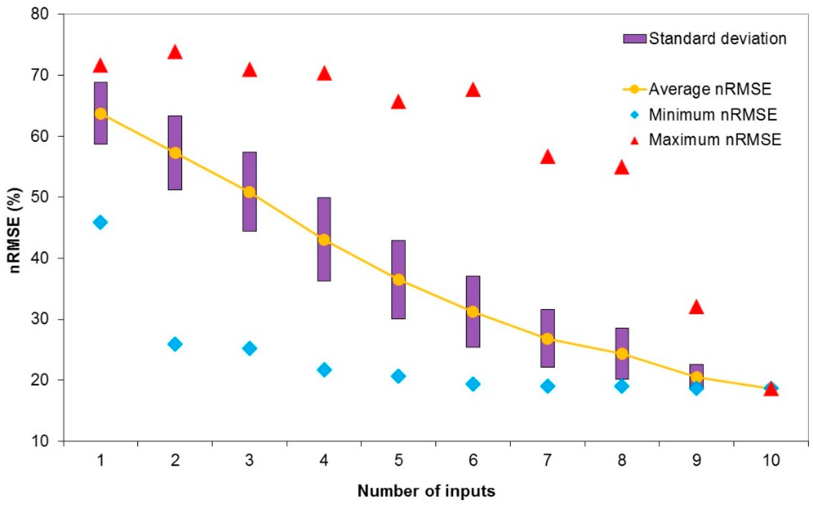
Figure 3 shows the average, minimum, and maximum values of nRMSE and the standard deviation versus the number of inputs.

The minimum nRMSE was obtained for the 10 inputs model with a value of 18.65% compared to 73.91% for the worst configuration (2 inputs: WD and WS).

Table 3. Best configurations according to the number of inputs for the Bouzareah site (1 = present data, 0 = absent data).

Nbr inputs	Rank	δ	${\mathit{\theta }}_{\mathit{z}}$	T	H	p	Pr	WS	WD	S	ETI	MAE Wh/m2	nMAE %	RMSE Wh/m2	nRMSE %	MBE Wh/m2
10	2	1	1	1	1	1	1	1	1	1	1	5.083	15.50	6.116	18.65	−0.084
9	1	1	1	1	1	1	1	1	1	1	0	5.083	15.50	6.115	18.65	0.011
9	3	1	1	1	1	1	0	1	1	1	1	5.118	15.61	6.152	18.76	−0.034
8	6	0	1	1	1	1	0	1	1	1	1	5.199	15.85	6.234	19.01	−0.018
8	7	1	0	1	1	1	1	1	0	1	1	5.209	15.88	6.245	19.04	−0.012
7	15	0	1	1	1	1	0	1	0	1	1	5.285	16.12	6.323	19.28	−0.038
7	24	1	1	1	1	1	0	1	0	1	0	5.358	16.34	6.399	19.51	−0.032
6	18	0	0	1	1	1	0	1	0	1	1	5.306	16.18	6.345	19.35	−0.081
6	32	0	0	1	1	1	0	1	0	1	1	5.415	16.51	6.457	19.69	−0.021
5	108	0	0	0	1	1	0	1	0	1	1	5.723	17.45	6.775	20.66	0.018
5	117	0	0	1	1	0	0	1	0	1	1	5.756	17.55	6.809	20.76	−0.015
4	196	0	0	1	1	0	0	0	0	1	1	6.066	18.50	7.128	21.74	−0.007
4	226	0	0	0	1	1	0	0	0	1	1	6.213	18.95	7.280	22.20	−0.018
3	360	0	0	0	1	0	0	0	0	1	1	7.162	21.84	8.257	25.18	−0.003
3	363	0	1	0	0	0	0	0	0	1	1	7.245	22.09	8.343	25.44	−0.005
2	372	0	0	0	0	0	0	0	0	1	1	7.389	22.53	8.491	25.89	0.003
2	379	0	1	0	0	0	0	0	0	1	0	8.086	24.66	9.209	28.08	0.062
1	753	0	1	0	0	0	0	0	0	0	0	13.762	41.97	15.058	45.92	0.062
1	754	0	0	0	0	0	0	0	0	0	1	13.780	42.02	15.076	45.97	−0.004

presents the two best configurations for the same number of inputs; as an example, for 9 inputs, 10 combinations were possible, and only the two best ones (from an nRMSE point of view) are reported in Table 3. The models were classified in descending order of performance (ranking).

Some models with a lower number of inputs can be better than models with a higher number of inputs. The declination, δ, appeared very rarely, WD and Pr never appeared, S was always present, and T, H, EHI, and p were often present; these 5 inputs had a relatively good R with GHI (but only 6% for temperature).

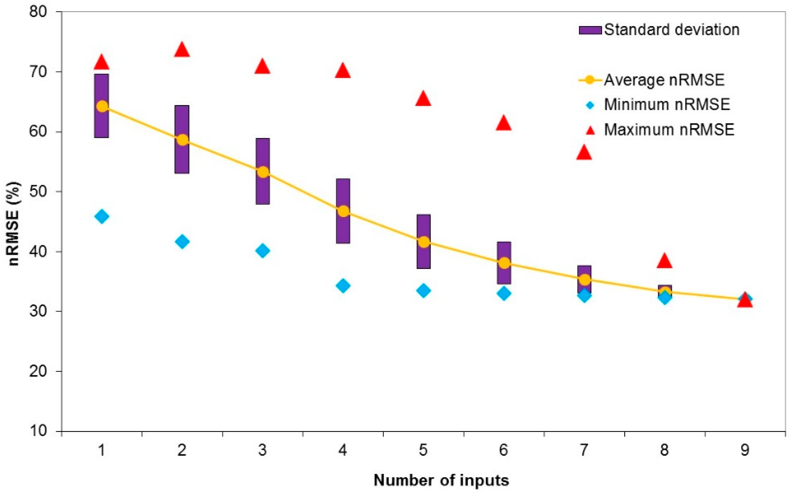
Without S (strongly linked with GHI), the best nRMSE dropped to 32.07% compared with 18.65% for the best configuration with 10 inputs.

Table 4. Best configurations according to the number of inputs (without S) (Bouzareah site). (1 = present data, 0 = absent data).

Nbr inputs	Rank	δ	${\mathit{\theta }}_{\mathit{z}}$	T	H	p	Pr	WS	WD	EHI	MAE Wh/m2	nMAE %	RMSE Wh/m2	nRMSE %	MBE Wh/m2
9	382	1	1	1	1	1	1	1	1	1	9.354	28.52	10.52	32.07	−1.142
8	383	0	1	1	1	1	1	1	1	1	9.427	28.75	10.59	32.29	−1.008
8	384	1	0	1	1	1	1	1	1	1	9.435	28.77	10.60	32.32	−1.058
7	389	1	0	1	1	1	1	1	0	1	9.536	29.08	10.70	32.64	−1.059
7	391	0	1	1	1	1	1	0	1	1	9.566	29.17	10.73	32.73	−1.010
6	398	0	1	1	1	1	1	0	0	1	9.661	29.46	10.83	33.03	−1.038
6	399	1	0	1	1	1	1	0	0	1	9.661	29.46	10.83	33.03	1.002
5	421	0	1	1	1	1	0	0	0	1	9.800	29.88	10.97	33.47	−1.872
5	426	0	0	1	1	1	0	0	1	1	9.838	30.00	11.01	33.58	−1.013
4	468	0	1	1	1	1	0	0	0	0	10.076	30.73	11.26	34.34	−1.042
4	496	0	0	1	1	1	0	0	0	1	10.226	31.18	11.41	34.80	−0.929
3	587	0	0	0	1	1	0	0	0	1	11.931	36.38	13.17	40.16	−0.816
3	605	0	1	0	1	1	0	0	0	0	12.120	36.96	13.37	40.75	0.918
2	635	0	0	0	1	0	0	0	0	1	12.415	37.86	13.67	41.68	1.033
2	650	0	1	0	1	0	0	0	0	0	12.566	38.32	13.83	42.16	1.063
1	753	0	1	0	0	0	0	0	0	0	13.762	41.97	15.06	45.92	1.062
1	754	0	0	0	0	0	0	0	0	1	13.780	42.02	15.07	45.97	−0.904

shows the results for the best configurations without S input.

Figure 4 shows the average, minimum, and maximum nRMSE values and the standard deviation versus the number of input data without S input.

The ANN reliability can be considered as correct, particularly when S was an input. Pr and WD had a low influence on GHI estimation (low correlation with GHI). The nRMSE of the 6-inputs model (T, H, p, WS, S, EHI) was 19.35% compared with the nRMSE of 10-inputs model with 18.65%; this combination had a good performance with a minimum of inputs.

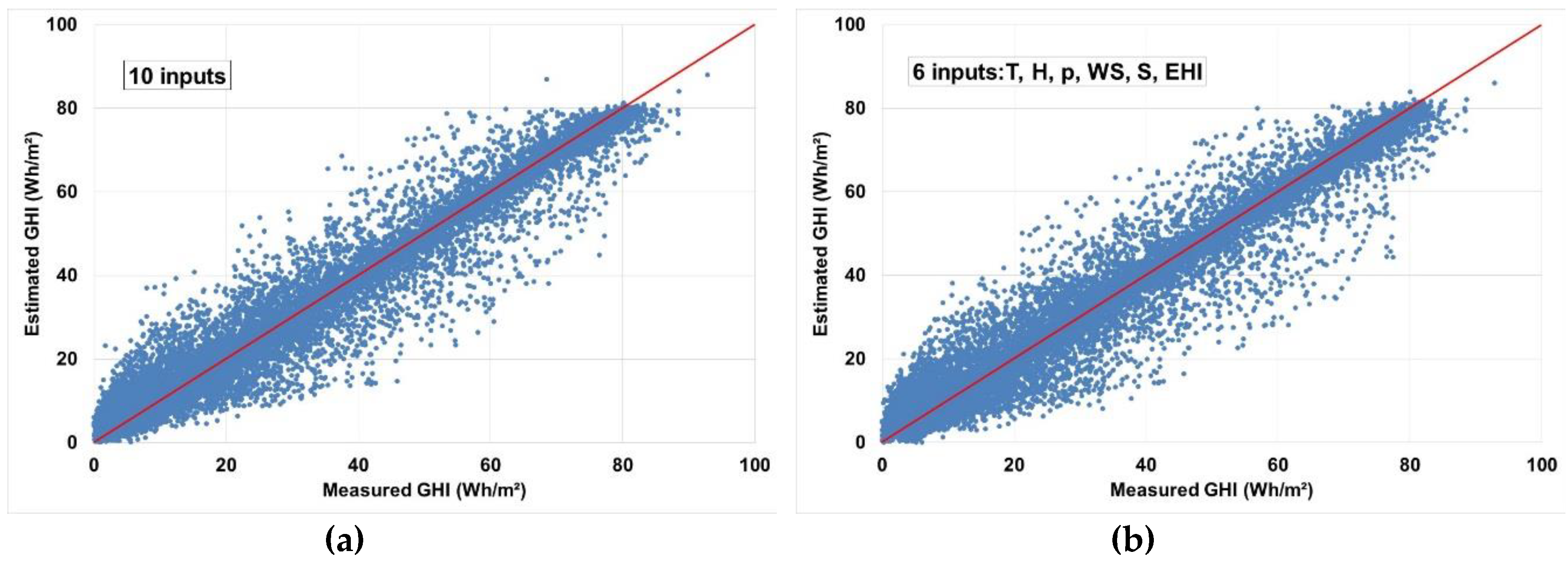
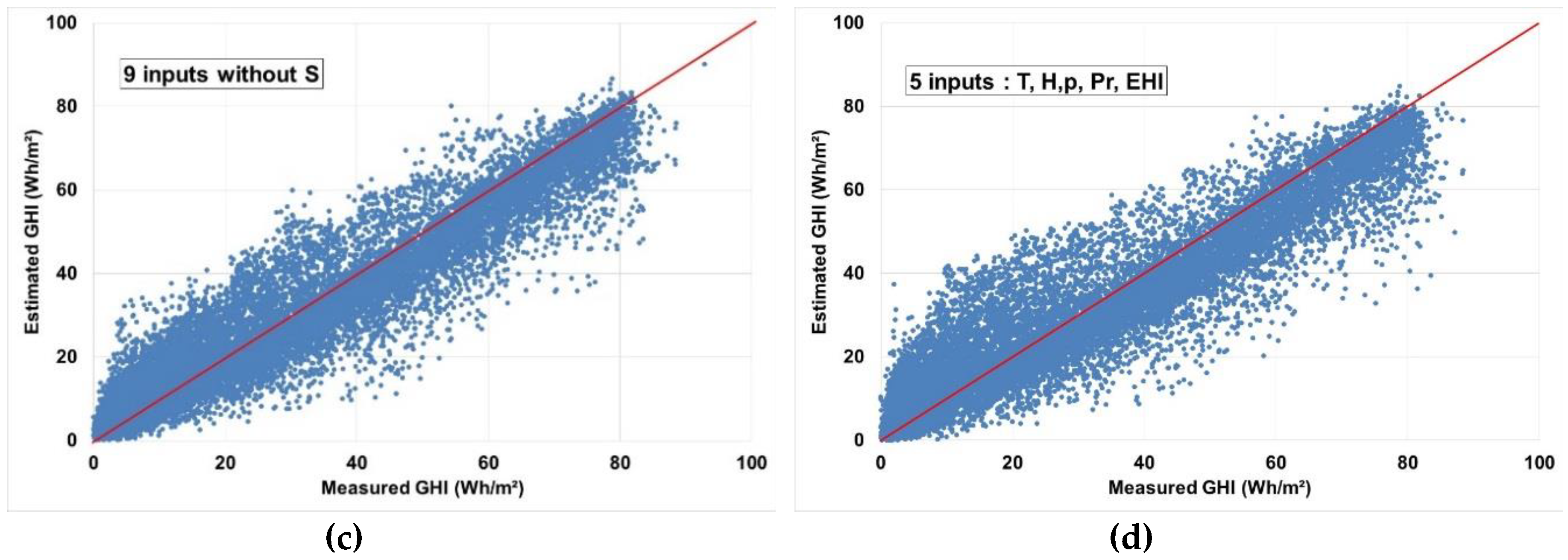
Estimated 5-min GHI is plotted versus the measured 5-min GHI for four architectures in Figure 5.

-

ANN structure with 10 inputs;

-

ANN structure with six inputs;

-

ANN structure with nine inputs without sunshine duration; and

-

best ANN structure with five inputs (without sunshine duration).

Few differences appeared between the ANN structure with 10 and six inputs in term of reliability and data dispersion. Without S, it appears clearly a more important spread of data compared with the results obtained with ANN structures with S in the inputs set. The performances of the best ANN structures without S for 5-min data were correct with an nMAE between 28.5% and 31% and an nRMSE between 32% and 35%.

The presence of some meteorological inputs in the “best” configurations seems sometimes surprising as WD and WS; it is difficult to understand the physical relations between GHI and other meteorological parameters. One of the major criticisms that could be levelled at the ANN model is that it is a black box model, allowing it to find some relations between data as often difficult to interpret, and ANN is a data driven method.

Even if some estimated data are far away from the real values, we can consider that the performance of this model is satisfying because determining GHI with a time granularity of 5-min from other meteorological data is a very complex task (high variability phenomenon and anisotropic aspect); keeping in mind that such a method is generally applied only for daily average values [5].

A bibliographical study [5] was realized on ANN methods used for such an estimation of GHI from exogenous meteorological data and this study showed that:

-

For the estimation of monthly mean values of daily GHI, the nRMSE was between 4.07% and 9.4%, but the process, on average, monthly, allows smoothing of the anisotropic effects and sometimes linear relationships are sufficient to link GHI with other parameters.

-

For the estimation of the daily GHI, nRMSE around 6% and nMAE around 5% were found. The time granularity was much higher than in our work.

Note that the determination coefficient (R²) between measured and estimated data was between 0.86 and 0.95 for the four graphs in Figure 5.

The mean bias error (MBE) was also computed for Figure 5 and was equal to −0.08 Wh/m², for 10 and six inputs, −1.14 Wh/m² for nine inputs without S, and −1.87 Wh/m² for five inputs; thus, all the ANN models slightly underestimated GHI.

5. Estimation of Tilted Global Irradiation (GTI) from Horizontal Global Irradiation (GHI)

In sizing or simulation software for solar systems, the solar collector inclination is introduced as an input and the horizontal solar data (generally hourly) collected from several meteorological stations are “tilted”. The accuracy and quality of GTI used as an input in these software have an impact on the reliability of the results.

It is difficult to develop a simple model for converting GHI into GTI [6] because the radiation received by a tilted plane includes the radiation reflected by the ground and scattered by the sky; this last component is difficult to estimate; when the collector is inclined, it sees only a part of the sky; moreover, the sky diffuse radiation depends on the inclination or orientation of the collector, on the elevation and azimuth of the sun, but also on the sky state with complex anisotropic effects [7,8]. The larger the time-step is, the more this anisotropy decreases (time-averaging and compensating effect) and tends towards an isotropic distribution; the shorter the time-step is, the more it is difficult to realize this conversion with good accuracy. The conversion of GHI to GTI is a complex issue often dealt with in the scientific literature [7,42,43,44,45,46].

5.1. Method

As in Section 4, the data used here were measured in Bouzareah.

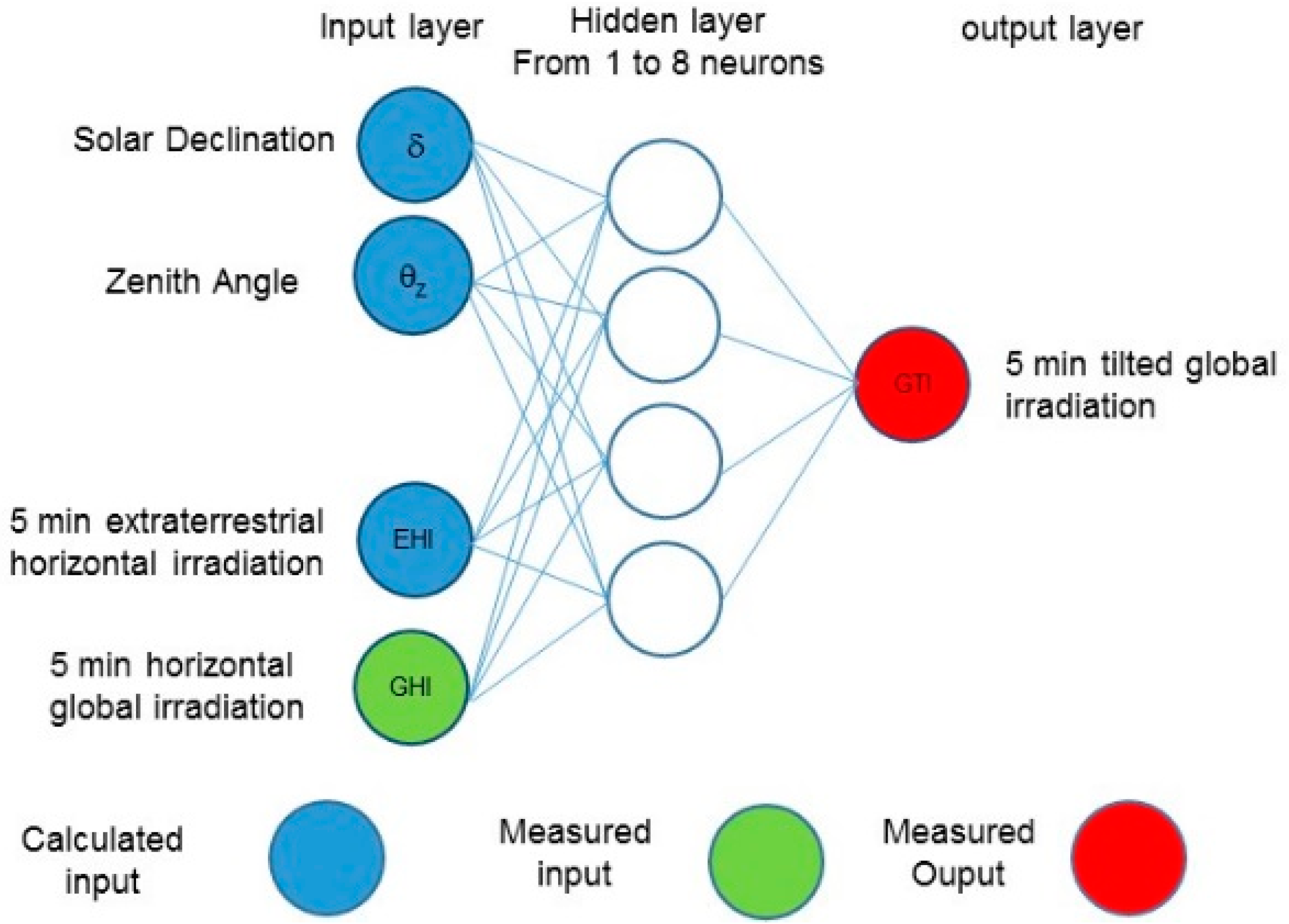
Four data, among them GHI, were used as input:

-

The declination representing the position of the Earth from the Sun depending on the day number;

-

the zenith angle characterizing the sun position, which influences the quantity and the quality of the sun radiation; when the sun is high in the sky (low zenith angle), the solar radiation is maximal (in clear skies). Moreover, as the optical path is minimal, the incident radiation is less absorbed;

-

the extraterrestrial irradiation, EHI, used as a reference; depending on sky conditions, several values of GTI correspond to the same GHI. In diffuse radiation models, the clearness or diffuse index are often used to characterize the sky. When the clearness index is high, then the sky is clear and GHI is mainly composed of BNI.

According to the rules described in Section 3.2, the number of hidden neurons in only one hidden layer will vary from one to eight. The ANN structure is shown in Figure 6.

5.2. Results

The five error metrics are presented in

Table 5. Average statistical parameters between measured and estimated global solar 5 min-irradiation on a 36.8° tilted plane for the station of Bouzareah. The bold line is the results for the best architecture.

Hidden Neurons Number	MAE	nMAE	RMSE	nRMSE	MBE
	Wh.m−2	%	Wh.m−2	%	Wh.m−2
1	5.94	16.32	6.89	18.93	−0.97
2	2.95	8.12	3.81	10.48	−0.29
3	2.80	7.71	3.65	10.04	−0.50
4	2.41	6.63	3.21	8.81	−0.31
5	2.56	7.04	3.47	9.54	−0.80
6	2.75	7.56	3.77	10.36	−1.14
7	2.68	7.38	3.68	10.12	−1.09
8	2.70	7.43	3.69	10.14	−1.12

(calculated on the basis of eight runs (each run corresponds to a different random weight initializing). The first column contains the number of neurons in the hidden layer.

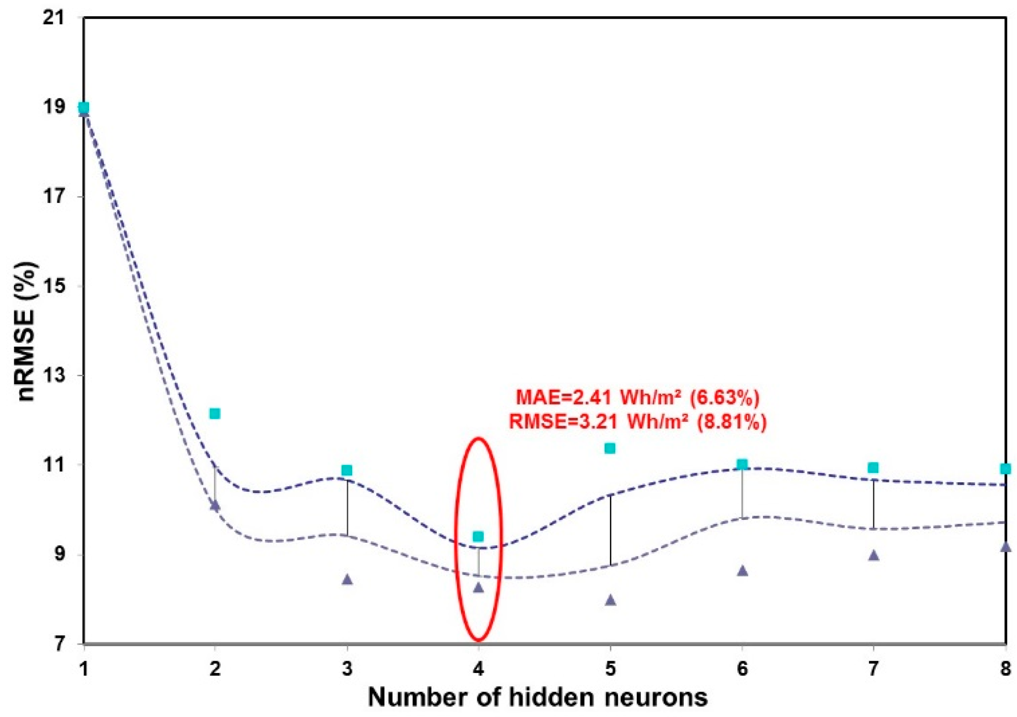
The nRMSE mean values and its corresponding standard deviation are presented in Figure 7 as an error-bar graph. An improvement appears until reaching four hidden neurons, then the nRMSE becomes almost constant and no improvement was observed. The dash points define the 95% confidence interval of the prediction errors (calculated based on eight runs per architecture), the triangles and squares are the minimum and maximum observed errors, respectively. We observed the same trend for the variation of the nMAE. The best configuration is encircled in red.

We conclude that an ANN with one hidden layer of four neurons is the best model. Moreover, it appears that the use of the azimuth does not provide any improvement. Thus, we will retain an ANN with four inputs and one hidden layer of four neurons, which have an average nRMSE of 8.81%, the best simulation with this ANN structure conduced to an nRMSE of 8.27%.

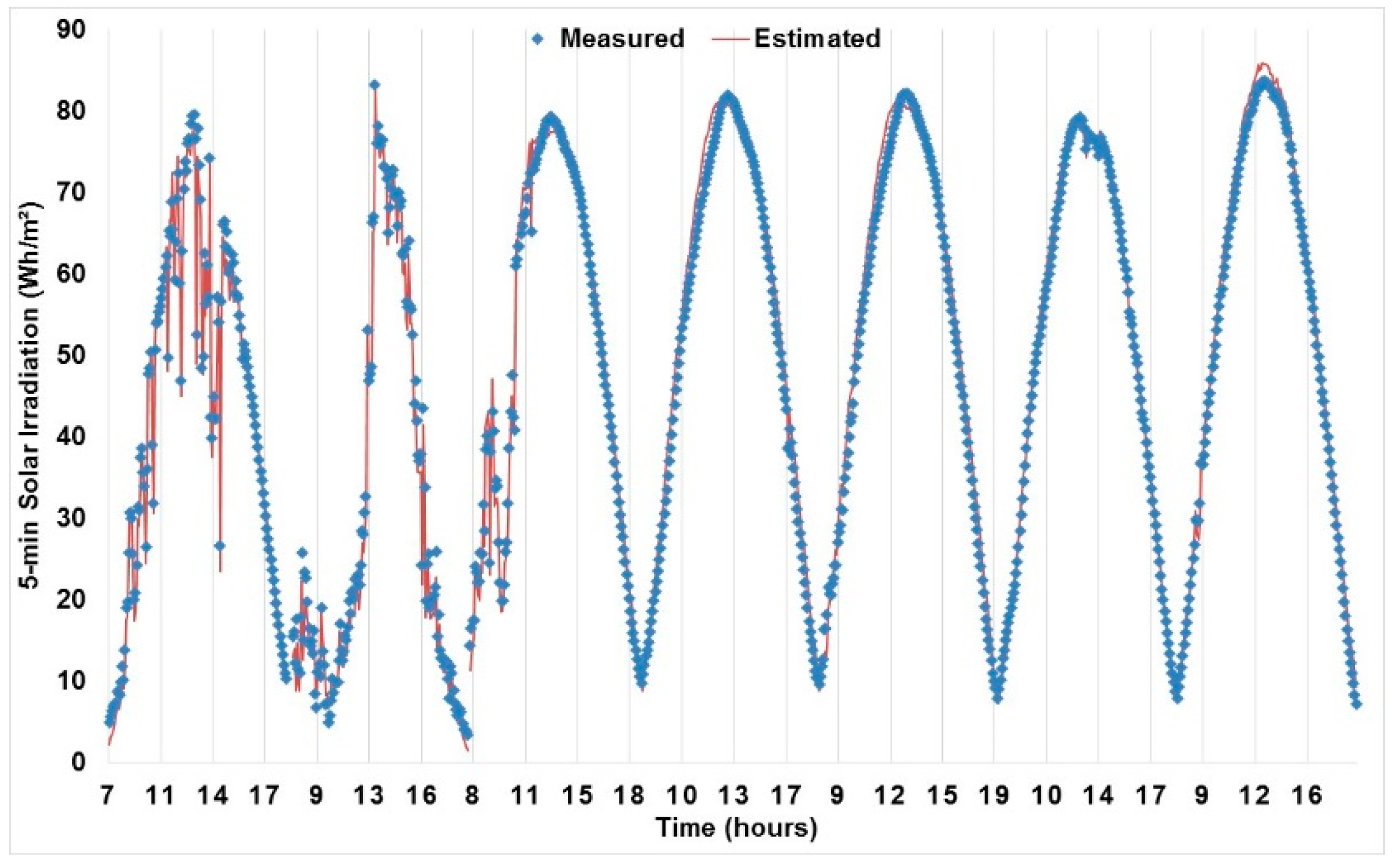
To illustrate the good reliability of this optimized MLP, a period of seven days unknown to the network was plotted with measured and calculated data in Figure 8.

A good relationship is observed between the modelled and measured data whatever the state of the sky is (clear, partially cloudy, and cloudy) because the nRMSE was under 10%, which is a good value for an nRMSE for such a short time step (5-min).

6. Forecasting of Hourly Direct Normal (DNI) and Horizontal Global (GHI) Irradiation for a Time Horizon from 1 h to 6 h

This forecasting work was realized from global horizontal (GHI) and normal beam (BNI) data measured at Odeillo, Pyrénées Orientales, located in the south of France (42°29 N, 2°01 E, 1550 m asl).

6.1. Stationnarization of Solar Data

Machine learning methods are efficient tools for forecasting time series with a stationary behavior. An MLP is a stationary model, which must use stationary data as input. To make solar irradiation time series stationary and to separate the climatic effects and the seasonal effects, the solar data are generally transformed in unitless variables called “clearness index”, and denoted kt; kt is the ratio of the solar radiation on the earth, GHI, to that outside the atmosphere, EHI, and defined by Equation (6) [35]:

$$kt=\frac{GHI}{EHI}$$

(7)

It is the clearness index series, kt, that induces randomness, caused by the diversity of atmospheric components (dusts, aerosols, clouds motion, and humidity) on the solar irradiation measured at the Earth‘s surface.

Numerous studies have showed that EHI can be efficiently replaced by the clear sky solar irradiation [22] taking into account the climatic conditions of the meteorological site; thus the clearness index is replaced by the clear sky index, k_g,cs, defined by:

$$k_{g,cs}=\frac{GHI}{GH{I}_{CS}}$$

(8)

with $GH{I}_{CS}$ the global horizontal solar irradiation in clear sky conditions.

For DNI, a similar index, k_d,CS [47,48], is defined by:

$$k_{d,cs}=\frac{DNI}{DN{I}_{CS}}$$

(9)

Various models of clear sky solar irradiations are available in the literature, which differ from each other mainly in the inputs needed by each model [49]. Solar irradiance models by clear sky denoted in the following clear sky models used meteorological variables (as ozone layer thickness, precipitable water, optical aerosol depth, etc.) and used solar geometry (solar elevation and air mass), using radiative transfer models to consider the absorption and diffusion effects of solar radiation into the atmosphere [50,51]. The most widely used clear sky model is the Solis model developed by Mueller et al. [52] and simplified by Ineichen [53], the European Solar Radiation Atlas (ESRA) model [54], and the Reference Evaluation on Solar Transmittance 2 (REST2) model [55].

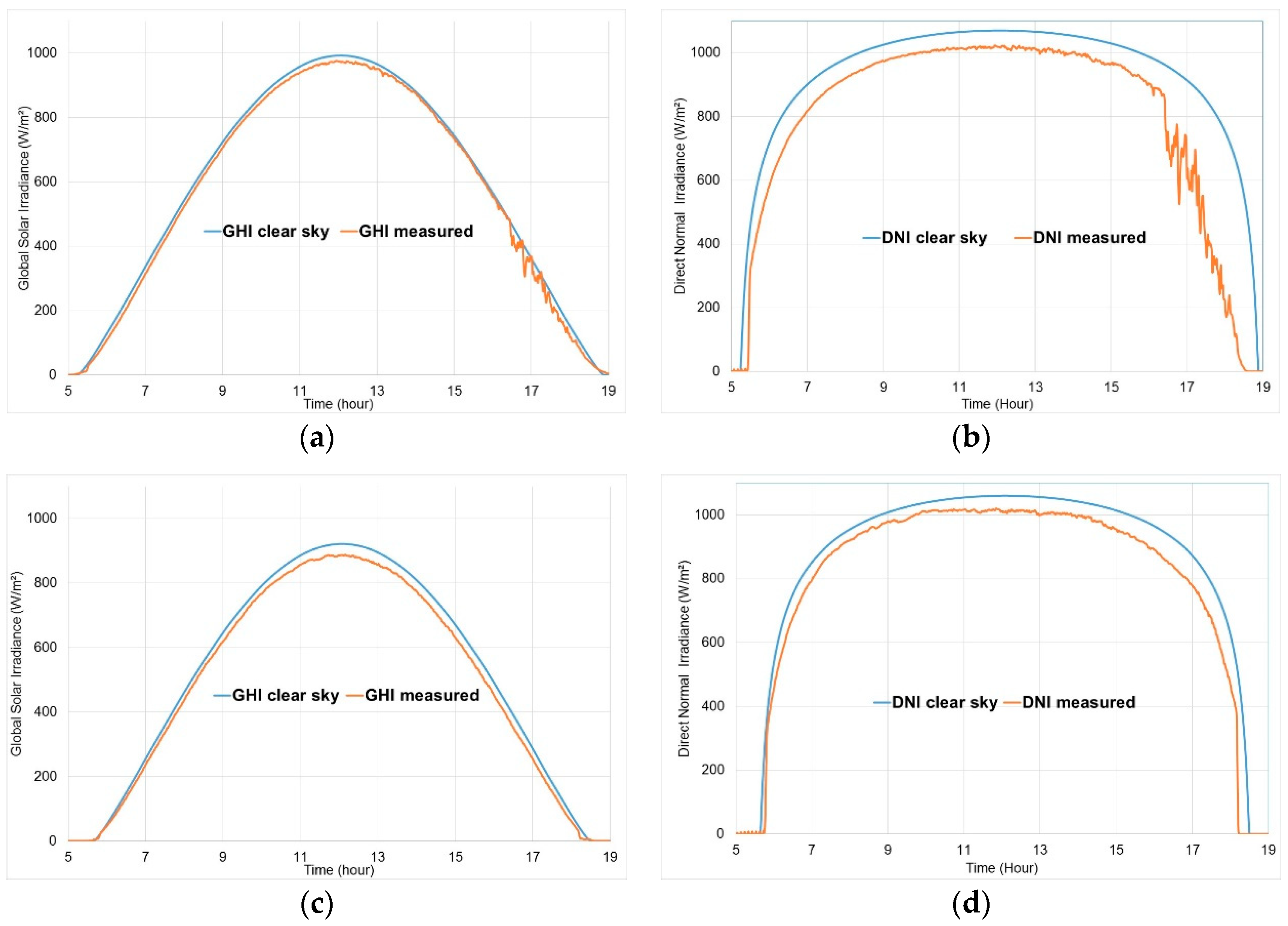
Thus, the simplified Solis clear sky model [53] was used here. It allowed calculations of the GHI_CS, and DNI_CS. This clear sky model was validated for each month by comparison with experimental solar radiation data measured in clear sky conditions. For illustration purposes, experimental and modelled solar irradiances by clear sky are plotted in Figure 9 for one day in April and in September.

6.2. Choice of the Number of Input Data

The purpose of Section 6 is to predict the future hourly solar irradiation (at different time horizons) based on the past observed data, i.e., mathematically:

$${\widehat{X}}_{t+h}=f\left(X_t,X_{t-1},X_{t-2},X_{t-3},\dots ,X_{t-n}\right)$$

(10)

A variable, X, with the symbol, $\widehat{}$, represents a forecasted data; without this symbol, X is a measured data. The solar data at future time step (t+h), ${\widehat{X}}_{t+h}$ is forecasted from the observed data X measured at the times (t, t − 1…, t − n); thus, the first objective consists of determining the value of n, i.e., the dimension of the input matrix; to do it, an auto mutual information method [56,57,58] was used. The auto mutual information is a property of the time series, it depends on each dataset and is characteristic of the degree of statistical dependence between $X_{t+h}$ and $X_{t-i}$ with 0 ≤ i ≤ n. It is a dimensionless quantity with units of bits. High mutual information indicates a large reduction in uncertainty about one random variable, $X_{t+h}$, given knowledge of another $\left(X_t,X_{t-1},X_{t-2},X_{t-3},\dots ,\right).$ The auto-mutual information method showed that the number of inputs (value of n in Equation (9)) for predicting GHI is six and for DNI, it is seven.

6.3. Methods

A first forecasting method, a naïve model, easy to implement and requiring no training step, i.e., no historical data set, was used as a reference model to compare it with more sophisticated models in terms of accuracy. It allowed us to see the improvement due to the use of the ANN forecaster.

The persistence model, the simplest forecasting model, assumes that the future value is identical to the previous one (Equation (10)). The persistence forecast accuracy decreases significantly with the forecasting horizon [59].

$${\widehat{X}}_{t+h}=X_t \mathrm{with}\mathrm{X}=\mathrm{GHI}\mathrm{or}\mathrm{DNI}$$

(10)

The smart persistence (SP) is an improved version of the persistence one taking into account the diurnal solar cycle: The clear sky solar radiation profile over the day was used [41]:

$${\widehat{X}}_{t+h}=X_t·\frac{X_{CS}{}_{t+h}}{X_{CS}{}_t}\mathrm{with}\mathrm{X}=\mathrm{GHI}\mathrm{or}\mathrm{DNI}$$

(12)

$X_{CS}{}_t$ is GHI or DNI for a clear sky condition calculated at time t. This smart persistence model was applied in this paper and used mainly as a reference model.

For the ANN model, as explained in Section 6.1, the clear sky index will be forecasted because it is a stationary series. Once the clear sky index is forecasted, the value of the forecasted solar irradiation, (${\widehat{GHI}}_{t+h}, or {\widehat{DNI}}_{t+h})$ is obtained by multiplying it by the calculated clear sky irradiation ($GH{I}_{CS}{}_{t+h} or DN{I}_{CS}{}_{t+h}).$

6.4. Results for GHI

Table 6. Performance metrics (in Wh/m² for RMSE, MAE, and MBE) for GHI (in bold the best predictor for each horizon and each error metric) (Odeillo site).

Metric	Model	h+1	h+2	h+3	h+4	h+5	h+6
RMSE	SP	97.72	132.41	157.08	176.48	193.06	202.66
	ANN	101.79	126.65	141.95	150.28	154.82	157.27
nRMSE	SP	21.67%	29.36%	34.82%	39.12%	42.79%	44.91%
	ANN	22.57%	28.08%	31.47%	33.31%	34.31%	34.85%
MAE	SP	56.97	80.82	98.70	112.83	124.64	130.85
	ANN	72.87	90.97	106.83	112.60	117.56	118.59
nMAE	SP	12.63%	17.92%	21.88%	25.01%	27.62%	28.99%
	ANN	16.16%	20.17%	23.68%	24.96%	26.05%	26.28%
MBE	SP	4.62	3.79	0.33	−4.63	9.42	−12.9
	ANN	−2.39	−5.67	7.12	10.14	12.32	14.7

gives the values of the error metrics calculated on the test data set (RMSE, MAE, and MBE are given in Wh.m⁻²).

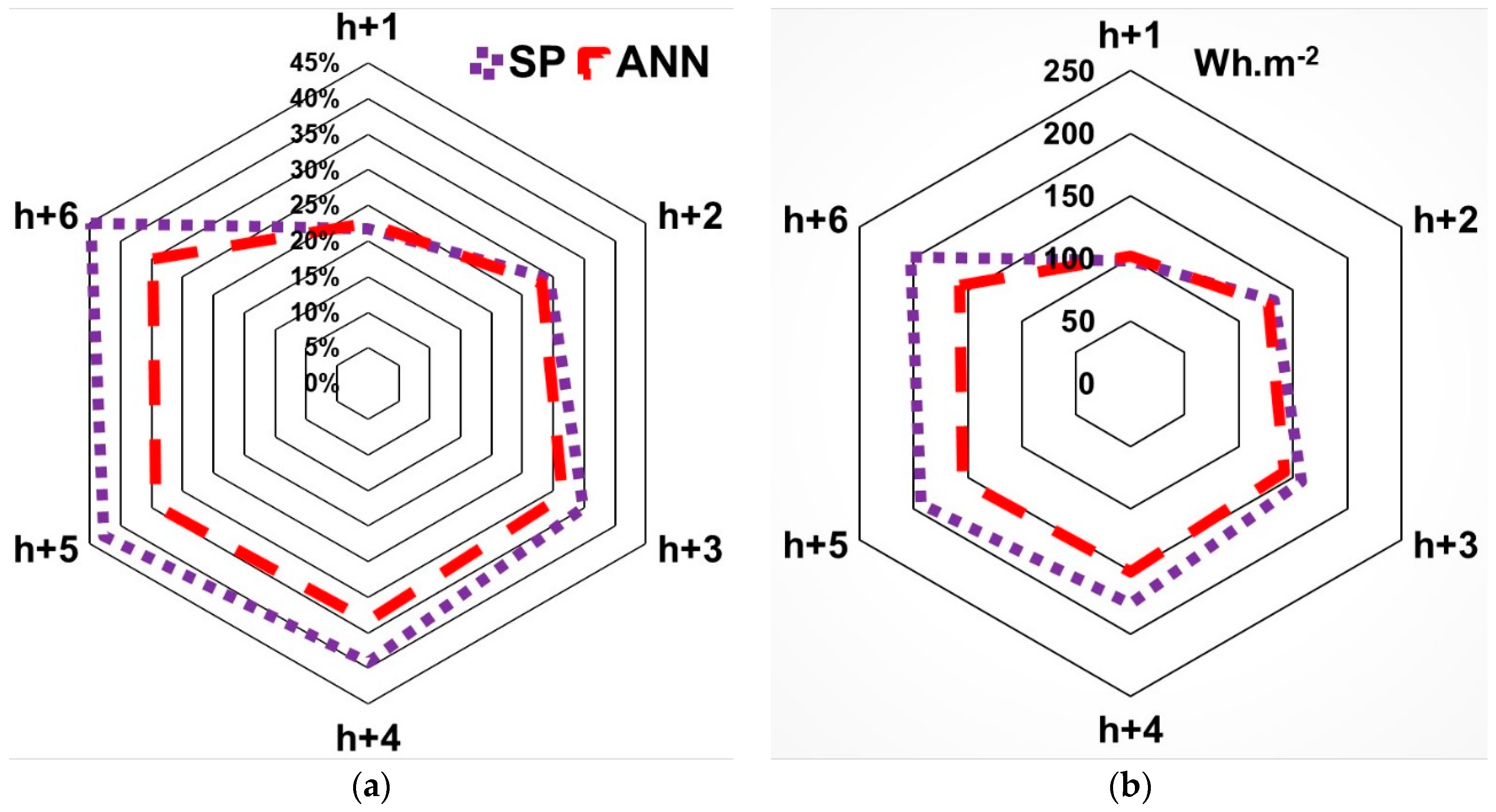
As the ranking of the model is always identical from a RMSE point of view or a MAE point of view, we only present in Figure 10 the results in terms of RMSE and nRMSE expressed in percentage.

The smart persistence, a naive model, was used as a reference. This model has a good RMSE and MAE for a time horizon, h+1, but its performances decrease rapidly with the time horizon. The gap in term of performances between ANN and SP increases with the time horizon.

6.5. Results for DNI

Table 7. Performance metrics (in Wh/m² for RMSE, MAE, and MBE) for DNI (in bold is the best predictor for each horizon and each error metric) (Odeillo site).

Metric	Model	h+1	h+2	h+3	h+4	h+5	h+6
RMSE	SP	207.86	287.64	338.86	378.19	412.67	434.51
	ANN	212.33	270.10	297.73	321.59	336.98	344.00
nRMSE	SP	37.42%	51.77%	60.98%	68.04%	74.23%	78.16%
	ANN	38.23%	48.62%	53.58%	57.85%	60.61%	61.88%
MAE	SP	125.24	187.12	230.34	266.01	298.23	317.71
	ANN	168.14	223.27	244.91	274.60	283.68	299.16
nMAE	SP	22.55%	33.68%	41.45%	47.85%	53.64%	57.15%
	ANN	30.27%	40.19%	44.07%	49.40%	51.02%	53.82%
MBE	SP	2.28	2.10	1.28	0.63	−0.58	−2.66
	ANN	3.34	2.76	−4.12	−6.15	−6.24	−6.88

gives the values of the performance metrics computed on the test data set (RMSE, MAE, and MBE are given in Wh.m⁻²) for DNI.

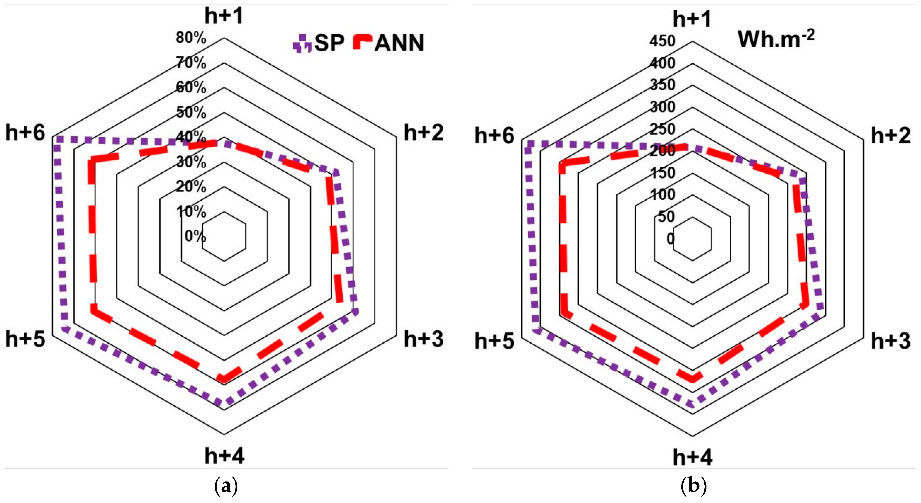
The results in terms of RMSE and nRMSE are presented in Figure 11 for BNI.

The DNI forecasting is more difficult and the models’ performances were less satisfying than with GHI particularly because DNI was more sensitive to meteorological conditions and because its variation was more rapid and of a greater magnitude than for GHI.

Some differences are noted in terms of ranking according to the metric used (nRMSE or nMAE), the nRMSE gives more importance to large gaps between predicted and measured data and generally the forecasting models were better compared in term of nRMSE than nMAE.

6.6. Comparison between GHI and DNI Forecasts

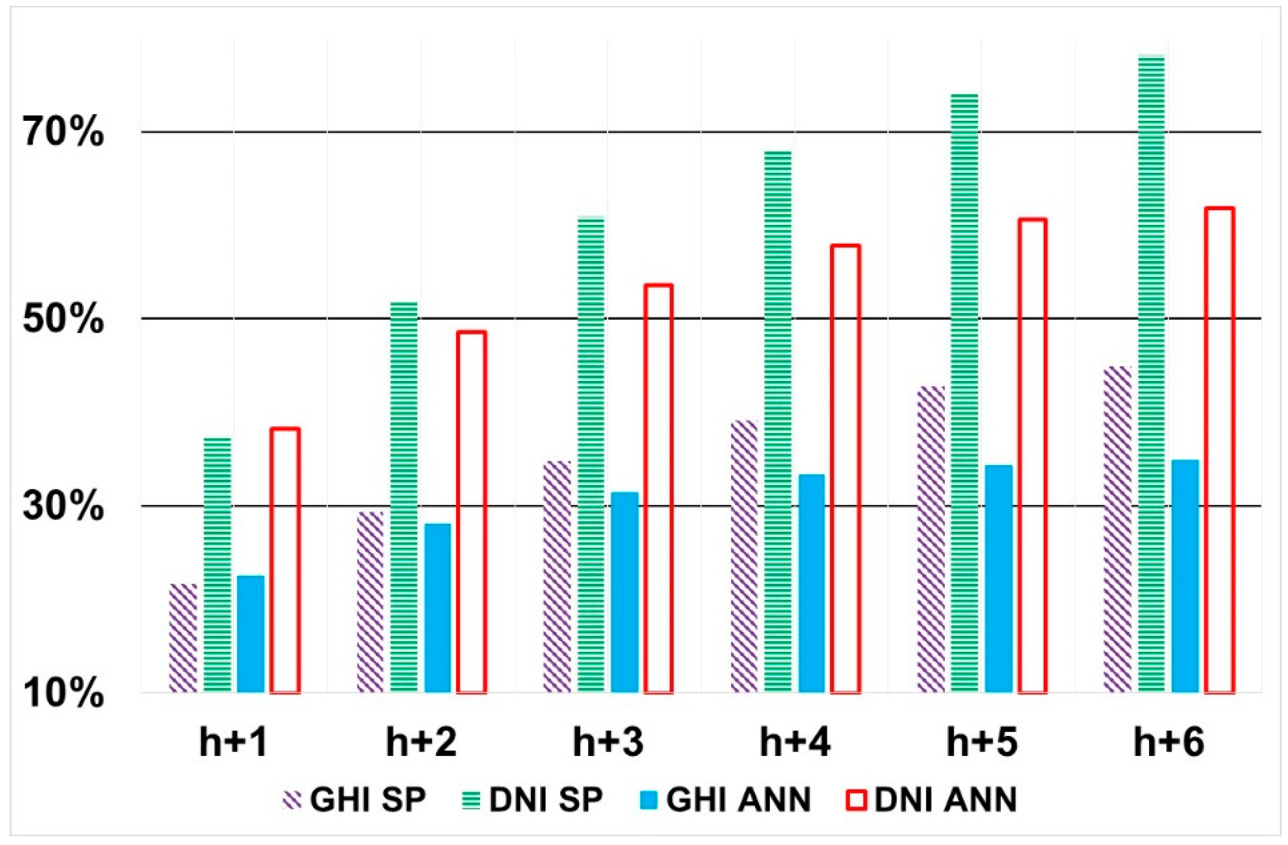
It is impossible to compare the performances of the models according to the solar component in terms of the absolute value of RMSE (or MAE) because the daily curve of GHI and DNI are very different in term of amplitude and form. Thus, we plotted in Figure 12 a comparison of the performances in term of nRMSE because it is the most common error metric used in the solar radiation prediction; in the case of Figure 11, as we compared two different solar radiations (GHI and DNI) with a different scale, the normalized value of RMSE seems to be the most adapted metric.

As previously underlined, GHI was forecasted with a better accuracy compared with DNI. It is probably due to the fact that in GHI, the two components, diffuse one and beam one, have compensating effects (when diffuse increases, beam decreases) and the variation rate of GHI is less rapid than for DNI. With SP and ANN methods, DNI is predicted with an nRMSE nearly twice as high than for GHI, but this difference was reduced when the forecast horizon increased and for (h+6), the accuracy for DNI prediction was the same than for GHI prediction.

Antonanzas et al. [50] reviewed the intra-day ahead forecast performances for PV production (using GHI as renewable resource) using different numerical prediction models. Various error metrics were used and calculated according to different definitions, moreover, the forecasting methods were applied in different meteorological stations; thus, it is very difficult to make a comparison of our results with the literature in these conditions.

A short bibliographical study [60] on DNI forecasting concludes that the DNI forecasting is obtained with a lower accuracy than for GHI forecasting and that only a small number of articles are written on the DNI forecasting at short time horizons as confirmed by Law et al. [20].

7. Conclusions

In this paper, the efficiency of the ANN method was shown for the estimation and the forecasting of solar irradiation.

Successively, several ANN models were developed:

-

An ANN model to determine the 5-min GHI from more available meteorological data (a maximum of seven measured meteorological data). The nRMSE of the optimized 6-inputs model was 19.35%.

-

An ANN model to compute the 5-min GTI from GHI with an accuracy around 8% for the optimal configuration.

-

At last, a forecasting ANN tool was developed to predict hourly DNI and GHI i for a time horizon from h+1 to h+6. The forecasting of hourly solar irradiation from h+1 to h+6 using ANN was realized with an nRMSE from 22.57% for h+1 to 34.85% for h+6 for GHI and an nRMSE from 38.23% for h+1 to 61.88% for h+6 for DNI.

ANN methods are very promising even if new artificial intelligence methods are in development, such as regression trees and random forest.

References

- Atwater, M.A.; Ball, J.T. A numerical solar radiation model based on standard meteorological observations. Sol. Energy 1978, 21, 163–170. [Google Scholar] [CrossRef]
- Hidalgo, F.G.; Martinez, R.F.; Vidal, E.F. Design of a Low-Cost Sensor for Solar Irradiance. Available online: http://oceanoptics.com (accessed on 25 November 2018).
- Paulescu, M.; Paulescu, E.; Gravila, P.; Badescu, V. Weather Modeling and Forecasting of PV Systems Operation, Green Energy and Technology; Ó Springer-Verlag: London, UK, 2013. [Google Scholar]
- World Radiation Data Center (WRDC). WRDC Online Archive, National Renewable Energy Laboratory, US Department of Energy. 2012. Available online: https://www.re3data.org (accessed on 3 May 2017).
- Dahmani, K.; Notton, G.; Voyant, C.; Dizene, R.; Nivet, M.L.; Paoli, C.; Tamas, W. Multilayer Perceptron Approach for estimating 5-min and hourly horizontal global radiation from exogenous meteorological data in locations without solar measurements. Renew. Energy 2016, 90, 267–282. [Google Scholar] [CrossRef]
- Behr, H.D. Solar radiation on tilted south-oriented surfaces: Validation of transfer-models. Sol. Energy 1997, 61, 399–413. [Google Scholar] [CrossRef]
- Robledo, L.; Soler, A. Modelling irradiance on inclined planes with an anisotropic model. Energy 1998, 23, 193–201. [Google Scholar] [CrossRef]
- Padovan, A.; Del Col, D. Measurement and modeling of solar irradiance components on horizontal and tilted planes. Sol. Energy 2010, 84, 2068–2084. [Google Scholar] [CrossRef]
- Hontoria, L.; Riesco, J.; Zufiria, P.; Aguilera, J. Improved generation of hourly solar radiation artificial series using neural networks. In Proceedings of the Engineering Applications of Neural Networks (EANN’99), Warsaw, Poland, 13–15 September 1999. [Google Scholar]
- Hontoria, L.; Aguilera, J.; Zufiria, P. Generation of hourly irradiation synthetic series using the neural network multilayer perceptron. Sol. Energy 2002, 72, 441–446. [Google Scholar] [CrossRef]
- Jiang, Y. Computation of monthly mean daily global solar radiation in China using artificial neural networks and comparison with other empirical models. Energy 2009, 34, 1276–1283. [Google Scholar] [CrossRef]
- Notton, G.; Paoli, C.; Ivanova, L.; Vasileva, S.; Nivet, M.L. Neural network approach to estimate 10-min solar global irradiation values on tilted plane. Renew. Energy 2013, 50, 576–584. [Google Scholar] [CrossRef]
- Elminir, H.K.; Azzam, Y.A.; Younes, F.I. Prediction of hourly and daily diffuse fraction using neural network, as compared to linear regression models. Energy 2007, 3, 1513–1523. [Google Scholar] [CrossRef]
- Heinemann, D.; Lorenz, E.; Girodo, M. Forecasting of solar Radiation. In Solar Energy Resource Management for Electricity Generation from Local Level to Global Scale; Nova Science Publishers: New York, NY, USA, 2006. [Google Scholar]
- Lauret, P.; Voyant, C.; Soubdhan, T.; David, M.; Poggi, P. A benchmarking of machine learning techniques for solar radiation forecasting in an insular context. Sol. Energy 2015, 112, 446–457. [Google Scholar] [CrossRef]
- McCandless, T.C.; Haupt, S.E.; Young, G.S. Short term solar radiation forecast using weather regime dependent artificial intelligence techniques. In Proceedings of the 2th Conference on Artificial and Computational Intelligence and its Applications to the Environmental Sciences, Atlanta, GA, USA, 2–6 February 2014. [Google Scholar]
- COST. Weather Intelligence for Renewable Energies (WIRE). Current State Report No.ES1002. 2012. Available online: www.cost.eu/actions/ES1002 (accessed on 8 May 2017).
- Diagne, M.; David, M.; Lauret, P.; Boland, J.; Schmutz, N. Review of solar irradiance forecasting methods and a proposition for small-scale insular grids. Renew. Sustain. Energy Rev. 2013, 27, 65–76. [Google Scholar] [CrossRef]
- Kalogirou, S.A.; Şencan, A. Artificial intelligence techniques in solar energy applications. In Solar Collectors and Panels, Theory and Applications; Manyala, R., Ed.; Intechopen Publisher: London, UK, 2010; ISBN 978-953-307-142-8. [Google Scholar]
- Law, E.W.; Prasad, A.A.; Kay, M.; Taylor, R.A. Direct normal irradiance forecasting and its application to concentrated solar thermal output forecasting—A review. Sol. Energy 2014, 108, 287–307. [Google Scholar] [CrossRef]
- Ghofrani, M.; Ghayekhloo, M.; Azimi, R. A novel soft computing framework for solar radiation forecasting. Appl. Soft Comput. 2016, 48, 207–216. [Google Scholar] [CrossRef]
- Iqbal, M. An Introduction to Solar Radiation; Academic Press: Don Mills, ON, Canada, 1983; ISBN 0-12-373752-4. [Google Scholar]
- Global Earth Observation System of Systems (GEOSS). Available online: www.earthobservations.org/geoss.php (accessed on 3 May 2017).
- David, M.; Ramahatana, F.; Trombe, P.J.; Lauret, P. Probabilistic forecasting of the solar irradiance with recursive ARMA and GARCH models. Sol. Energy 2016, 133, 55–72. [Google Scholar] [CrossRef] [Green Version]
- Notton, G.; Voyant, C. Forecasting of Intermittent Solar Energy Resource. In Advances in Renewable Energies and Power Technologies; Yahyaoui, I., Ed.; Elsevier Science: Amsterdam, The Netherlands, 2018; pp. 77–109. ISBN 978-012-8131855. [Google Scholar]
- Sperati, S.; Alessandrini, S.; Pinson, P.; Kariniotakis, G. The “Weather Intelligence for Renewable Energies” Benchmarking Exercise on Short-Term Forecasting of Wind and Solar Power Generation. Energies 2015, 8, 9594–9619. [Google Scholar] [CrossRef] [Green Version]
- Haykin, S. Neural Networks: A Comprehensive Foundation, 2nd ed.; Prentice-Hall: Upper Saddle River, NJ, USA, 1999. [Google Scholar]
- Yildiz, N. Layered feedforward neural network is relevant to empirical physical formula construction: A theoretical analysis and some simulation results. Phys. Lett. A 2005, 345, 69–87. [Google Scholar] [CrossRef]
- Mellit, A.; Benghanem, M.; Hadj Arab, A.; Guessoum, A. An adaptive artificial neural network model for sizing stand-alone photovoltaic systems: Application for isolated sites in Algeria. Renew. Energy 2005, 30, 1501–1524. [Google Scholar] [CrossRef]
- Mellit, A.; Pavan, A.M. A 24-h forecast of solar irradiance using artificial neural network: Application for performance prediction of a grid-connected PV plant at Trieste, Italy. Sol. Energy 2010, 84, 807–821. [Google Scholar] [CrossRef]
- Abraham, A. Artificial Neural Networks. Handbook for Measurement Systems Design; Sydenham, P., Thorn, R., Eds.; John Wiley and Sons Ltd.: London, UK, 2005; pp. 901–908. ISBN 0-470-02143-8. [Google Scholar]
- Krishnaiah, T.; Srinivasa Rao, S.; Madhumurthy, K.; Reddy, K.S. Neural network approach for modelling global solar radiation. J. Appl. Sci. Res. 2007, 3, 1105–1111. [Google Scholar]
- Alam, S.; Kaushik, S.C.; Garg, S.N. Assessment of diffuse solar energy under general sky condition using artificial neural network. Appl. Energy 2009, 86, 554–564. [Google Scholar] [CrossRef]
- Cybenko, G. Approximation by superposition of sigmoidal function. Math. Control Signals Syst. 1989, 2, 303–314. [Google Scholar] [CrossRef]
- Wierenga, B.; Kluytmans, J. Neural nets versus marketing models in time series analysis: A simulation study. In Proceedings of the 23th Annual Conference of the European Marketing Academy, Maastricht, The Netherlands, 17–20 May 1994; pp. 1139–1153. [Google Scholar]
- Venugopal, V.; Baets, W. Neural networks and statistical techniques in marketing research: A conceptual comparison. Mark. Intell. Plan. 1994, 12, 30–38. [Google Scholar] [CrossRef]
- Shepard, R.N. Neural nets for generalization and classification: Comment on Staddon and Reid. Psychol. Rev. 1990, 97, 579–580. [Google Scholar] [CrossRef] [PubMed]
- Wiens, T.S.; Dale, B.C.; Boyce, M.S.; Kershaw, G.P. Three way k-fold cross-validation of resource selection functions. Ecol. Model. 2008, 212, 244–255. [Google Scholar] [CrossRef]
- Kuhn, M.; Johnson, K. Applied Predictive Modelling; Springer: Berlin/Heidelberg, Germany, 2013. [Google Scholar]
- Cigizoglu, H.K.; Kişi, Ö. Flow prediction by three back propagation techniques using k-fold partitioning of neural network training data. Hydrol. Res. 2005, 36, 49–64. [Google Scholar] [CrossRef]
- Voyant, C.; Soubdhan, T.; Lauret, P.; David, M.; Muselli, M. Statistical parameters as a means to a priori assess the accuracy of solar forecasting models. Energy 2015, 90, 671–679. [Google Scholar] [CrossRef] [Green Version]
- Wenxian, L.; Wenfeng, G.; Shaoxuan, P.; Enrong, L. Ratios of global radiation on a tilted to horizontal surface for Yunnan province. China. Energy 1995, 20, 723–728. [Google Scholar] [CrossRef]
- Li, D.H.W.; Lau, C.C.S.; Lam, J.C. Predicting daylight illuminance on inclined surfaces using sky luminance data. Energy 2005, 30, 1649–1665. [Google Scholar] [CrossRef]
- Cheng, C.L.; Chan, C.Y.; Chen, C.L. An empirical approach to estimating monthly radiation on south-facing tilted planes for building application. Energy 2006, 31, 2940–2957. [Google Scholar] [CrossRef]
- De Rosa, A.; Ferraro, V.; Kaliakatsos, D.; Marinelli, V. Calculating diffuse illuminance on vertical surfaces in different sky conditions. Energy 2008, 33, 1703–1710. [Google Scholar] [CrossRef]
- Pandey, C.K.; Katiyar, A.K. A note on diffuse solar radiation on a tilted surface. Energy 2009, 34, 1764–1769. [Google Scholar] [CrossRef]
- Linares-Rodríguez, A.; Ruiz-Arias, J.A.; Pozo-Vázquez, D.; Tovar-Pescador, J. Generation of synthetic daily global solar radiation data based on ERA-Interim reanalysis and artificial neural networks. Energy 2011, 36, 5356–5365. [Google Scholar] [CrossRef]
- Kaur, A.; Nonnenmacher, L.; Pedro, H.T.C.; Coimbra, F.M. Benefits of solar forecasting for energy imbalance markets. Renew. Energy 2016, 86, 819–830. [Google Scholar] [CrossRef]
- Badescu, V.; Gueymard, C.A.; Cheval, S.; Oprea, C.; Baciu, M.; Dumitrescu, A.; Iacobescu, F.; Milos, J.; Rada, C. Computing global and diffuse solar hourly irradiation on clear sky. Review and testing of 54 models. Renew. Sustain. Energy Rev. 2012, 16, 1636–1656. [Google Scholar] [CrossRef]
- Antonanzas, J.; Osorio, N.; Escobar, R.; Urraca, R.; Martinez-de-Pison, F.J.; Antonanzas-Torres, F. Review of photovoltaic power forecasting. Sol. Energy 2016, 136, 78–111. [Google Scholar] [CrossRef]
- Ineichen, P. Validation of models that estimate the clear sky global and beam solar irradiance. Sol. Energy 2016, 132, 332–344. [Google Scholar] [CrossRef] [Green Version]
- Mueller, R.; Dagestad, K.; Ineichen, P.; Schroedter-Homscheidt, M.; Cros, S.; Dumortier, D. Rethinking satellite-based solar irradiance modeling: The SOLIS clear-sky module. Remote Sens. Environ. 2004, 91, 160–174. [Google Scholar] [CrossRef]
- Ineichen, P. A broadband simplified version of the Solis clear sky model. Sol. Energy 2008, 82, 758–762. [Google Scholar] [CrossRef]
- Rigollier, C.; Bauer, O.; Wald, L. On the clear sky model of the ESRA—European Solar Radiation Atlas—with respect to the Heliosat method. Sol. Energy 2000, 68, 33–48. [Google Scholar] [CrossRef]
- Gueymard, C.A. REST2: High-performance solar radiation model for cloudless-sky irradiance, illuminance, and photosynthetically active radiation—Validation with a benchmark dataset. Sol. Energy 2008, 82, 272–285. [Google Scholar] [CrossRef]
- Huang, D.; Chow, T.W.S. Effective feature selection scheme using mutual information. Neurocomputing 2005, 63, 325–343. [Google Scholar] [CrossRef]
- Jiang, A.H.; Huang, X.C.; Zhang, Z.H.; Li, J.; Zhang, Z.Y.; Hua, H.X. Mutual information algorithms. Mech. Syst. Signal Process. 2010, 24, 2947–2960. [Google Scholar] [CrossRef]
- Parviz, R.K.; Nasser, M.; Motlagh, M.R.J. Mutual Information Based Input Variable Selection Algorithm and Wavelet Neural Network for Time Series Prediction. In Proceedings of the International Conference on Artificial Neural Networks (ICANN 2008), Prague, Czech Republic, 3–6 September 2008; Kůrková, V., Neruda, R., Koutník, J., Eds.; Springer: Berlin/Heidelberg, Germany, 2008; pp. 798–807. [Google Scholar]
- Huang, R.; Huang, T.; Gadh, R.; Li, N. Solar generation prediction using the ARMA model in a laboratory-level micro-grid. In Proceedings of the IEEE Third International Conference on Smart Grid Communications (SmartGridComm), Tainan, Taiwan, 5–8 November 2012; pp. 528–533. [Google Scholar]
- Benali, L.; Notton, G.; Fouilloy, A.; Voyant, C.; Dizene, R. Solar radiation forecasting using artificial neural network an random forest methods: Application to normal beam, horizontal diffuse and global components. Renew. Energy 2019, 132, 871–884. [Google Scholar] [CrossRef]
Figure 1.
Architecture of an artificial neuron and a multi-layered neural network.
Figure 2.
ANN structure for GHI estimation.
Figure 3.
Average, minimum, and maximum values of the nRMSE and its standard deviation versus the number of inputs (Bouzareah site).
Figure 4.
Average, minimum, and maximum values of the nRMSE and its standard deviation versus the number of inputs without S as input (Bouzareah site).
Figure 5.
Estimated 5-min GHI versus measured 5-min GHI for various ANN architectures (Bouzareah site); (a) using 10 inputs; (b) using 6 inputs (with S); (c) using 9 inputs (without S); (d) using 5 inputs (without S).
Figure 6.
ANN architectures for the estimation of ETI.
Figure 7.
nRMSE evolution vs the number hidden neurons (Bouzareah site).
Figure 8.
Validation of the model for seven randomly chosen days (Bouzareah site).
Figure 9.
Experimental and modelled solar irradiance curves in clear sky conditions (hour in true solar time) (Odeillo site), (a) GHI, April; (b) DNI, April; (c) GHI, September; (d) DNI, September.
Figure 10.
Comparison of forecasting models for various horizons for hourly GHI (Odeillo site); (a) in term of nRMSE; (b) in term of RMSE.
Figure 11.
Comparison of forecasting models for various horizons for hourly DNI (Odeillo site); (a) in terms of nRMSE; (b) in term of RMSE.
Figure 12.
Comparison of forecasting models for GHI and DNI in terms of nRMSE (Odeillo site).