Optimal Energy Routing Design in Energy Internet with Multiple Energy Routing Centers Using Artificial Neural Network-Based Reinforcement Learning Method

Abstract

In order to cope with the energy crisis, the concept of an energy internet (EI) has been proposed as a novel energy structure with high efficiency which allows full play to the advantages of multi-energy coupling. In order to adapt to the multi-energy coupled energy structure and achieve flexible conversion and interaction of multi-energy, the concept of energy routing centers (ERCs) is proposed. A two-layered structure of an ERC is established. Multi-energy conversion devices and connection ports with monitoring functions are integrated in the physical layer which allows multi-energy flow with high flexibility. As for the EI with several ERCs connected to each other, energy flows among them are managed by an energy routing controller located in the information layer. In order to improve the efficiency and reduce the operating cost and environmental cost of the proposed EI, an optimal multi-energy management-based energy routing design problem is researched. Specifically, the voltages of the ERC ports are managed to regulate the power flow on the connection lines and are restricted on account of security operations. An artificial neural network (ANN)-based reinforcement learning algorithm was proposed to manage the optimal energy routing path. Simulations were done to verify the effectiveness of the proposed method.

1. Introduction

With the aggravation of the shortage of fossil fuels and the growing concerns over environmental pollution, current power grids are caught in a dilemma between the increasing power demand of users and environmental protection. What is more, users’ demands for energy tend to be diversified and the efficiency of multiple types of energy needs to be improved. Consequently, the concept of energy internet (EI) is proposed as a feasible way to solve the existing problems [1,2]. Energy internet can be assumed as a multi-energy coupled network with high permeability of renewable energy resources. In addition, to promote efficiency, a distributed energy supply structure is substituted for a traditional centralized generation structure in the EI [3].

During the pursuit of an economic and environmentally-friendly energy system, energy management problems were researched. Energy management problems are usually concluded as an optimization problem with one or more objective functions and several constraints. Many research works have been conducted under the background of EI. Operating cost is one of most common objective functions used in energy management problems [4,5]. However, with the growth of attention on environmental protection, multi-objective energy management which considers carbon emissions and operational cost simultaneously has been studied in many research works [6,7].

In order to fit the decentralized structure and realize flexible energy transmission, the concept of an energy router was first introduced in the smart grid scenario [8], where the structure of the energy router as proposed and its functions were discussed. As the key device of EI, various types of studies have been conducted based on energy routers, such as optimal location selection [9,10], stability control [11], and structural design [12]. There are a few studies conducting research on energy-router-based energy management. In Reference [13], solid-state transformer was used as an energy router, and an optimal economic energy-management-based energy routing strategy, which reduced consumption of grid power, was proposed. In Reference [14], a local area energy network containing several energy routers was proposed, and the energy routing algorithm was formulated to find the routing path with the lowest power loss. However, the study only considered the routing management for electrical energy, and other types of energy were not considered. Thus, this paper aims to consider various types of energy coupled with EI, such that an energy-management-based energy routing design for multiple types of energy is studied.

Reinforcement learning as a main class of machine learning has been adopted in various fields of energy systems including optimal control [15,16,17], fault diagnosis [18], reactive power control and optimization [19,20], etc. When it comes to the issue of energy management, as for complex energy networks with high penetration of renewable energy, challenges brought by its randomness affect the optimal energy management. Due to the fluctuant characteristic of renewable energy sources, the existing literature makes forecasts of loads and generation units based on long-term data during energy management processes. However, acquiring accurate a priori information of generation devices and loads is not straightforward and restricts its applications. Besides, forecasts based on a large amount of data brings about an increase on the computational burden. In contrast, reinforcement learning method shows high efficiency in solving such problems due to its features being model-free. Reinforcement learning does not rely on a priori knowledge, which increases the flexibility of its application on energy management in complex energy systems. Therefore, reinforcement learning has been adapted to energy management in recent years. A dynamic energy management system for microgrids has been established in Reference [21] and reinforcement learning method has been used to realize optimal control of the whole system. In Reference [22], by designing a marketing auction mechanism, a reinforcement learning algorithm was adopted to obtain an energy management strategy with minimized economic cost. A study of energy management in an office building with renewable energy resources was carried out in Reference [23], and an echo-state based reinforcement learning method was used to manage the output power of devices in an office building. In these studies, only electrical power management was involved and only economical cost was considered. However, as for multi-energy coupled EI, thermal power is involved so that environmental cost [24] needs to be taken into consideration in this paper. What is more, considering the physical entities, secure operation of the system is necessary to be discussed at the same time. Reinforcement learning method is adopted in this paper to schedule an energy-management-based energy routing path, and an artificial neural network is combined with reinforcement learning to avoid the curse of dimension.

To summarize, the major contributions of this paper are:

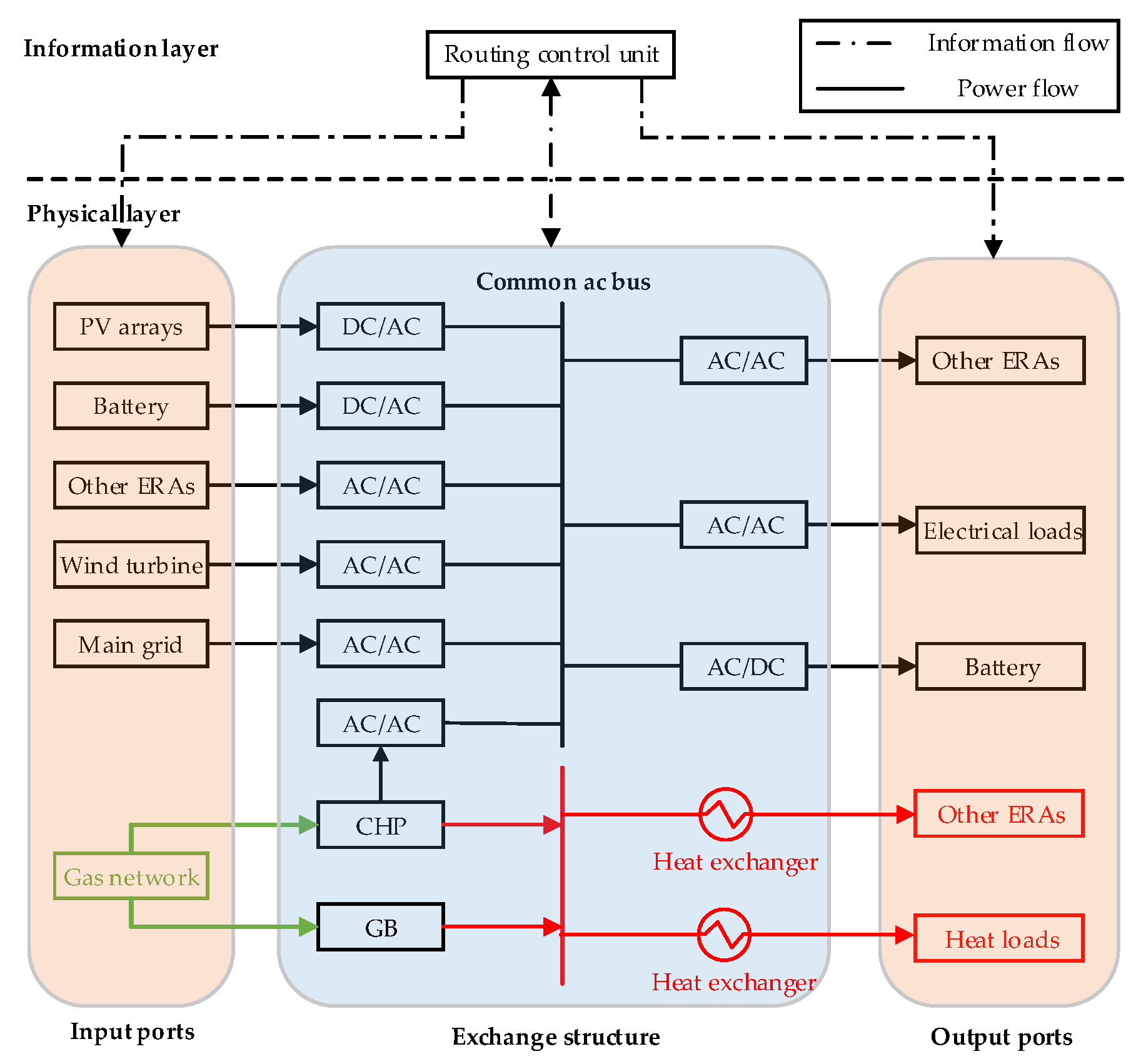
• In an environment of multi-energy coupled EI, the concept of energy routing center (ERC) is proposed for the first time. As a core energy interaction entity, a two-layered structure is designed for ERC and their corresponding functions are depicted in this paper. In the physical layer, multi-energy conversion devices and connection ports allowing plug-and-play of multi-energy users are integrated. In the information layer, an energy routing unit is embedded to schedule energy management and routing design. The ERC provides users with a novel integrated multi-energy conversion node which improves the flexibility of energy interaction in EI.
• Considering the physical connections among ERCs in EI, a multi-energy management-based optimal energy routing design problem considering operating cost, environmental cost, and security operation is researched in this paper. Specifically, in order to reduce the difficulty of control in reality, the voltages of ERC ports are managed to regulate power flow. Considering reality factors such as physical connection structure makes energy management problems adapt to the EI circumstances better.
• Due to the fluctuations of renewable resources and users’ demands, the topological relationship between load and source in multi-energy system varies frequently, therefore, reinforcement learning combined with artificial neural network (ANN) is adopted in the optimal energy routing design to form an energy routing path with high efficiency and lower costs. As a model free method, reinforcement learning does not rely on the priori knowledge of the environment which shows high efficiency.

The remainder of the paper is organized as follows. Section 2 establishes a structure of the EI, which consists of multiple ERCs and identifies the inner structure and functions of the ERCs. Section 3 defines the connection weights of connection lines between ERCs on account of operating cost, environmental cost, and power transmission loss. In Section 4, an ANN-based Q-learning algorithm is adopted to solve energy-management-based energy routing design problems. Simulations were performed in Section 5 to validate the effectiveness of the proposed algorithm. Section 6 concludes this paper.

2. Establishment of Energy Internet with Energy Routing Centers

2.1. Structure of Energy Internet with Energy Routing Centers

In the EI, multi-types of energy are coupled together and different energy users bring about diversified energy demands. In order to promote the flexibility of user side and enhance the absorption capacity of renewable energy, the EI is divided into several energy regions. Different energy regions are connected through ERCs. The structure of the EI containing multiple ERCs is shown in Figure 1.

As shown in Figure 1, energy supply facilities including gas-fired combined heat and power (CHP), gas boiler (GB), photovoltaic, battery, and wind turbine are connected to ERCs. The ERCs are connected together through power lines and thermal pipelines which allows bi-directional energy interaction. That is to say, energy regions possess the ability of supplying energy and are able to act as energy suppliers during the energy interaction process. When a region has excess energy, rather than store the excess energy in storage devices, it transfers energy to other regions which are in short supply of energy first. Therefore, the flexibility of the demand side and the absorption capacity for renewable energy are promoted at the same time.

2.2. Architecture and Functions of Energy Routing Center

In order to realize flexible energy conversion and power dispatch of multi-types of energy, a multi-energy coupled network is proposed in this paper. The basic structure of the ERC is shown in Figure 2.

As can be seen in Figure 2, an energy routing center is composed of an energy routing control unit, an energy conversion structure, and several input and output ports. In order to illustrate the structure of the ERC clearly, the ERC is divided into the information layer and the physical layer. The energy routing control unit is located in the information layer; it exchanges information with devices located in the physical layer. The control unit receives information from the exchange structure and transfers control signals to the input/output ports. What is more, as an indispensable part of the ERC, the energy routing control unit undertakes functions of energy management and routing design. Energy management mainly focuses on the energy transmission between different ERCs, that is to say, each energy routing control unit formulates a scheme of its output energy. As for energy routing design, due to the restrictions of real topology of the energy network and upper limit of energy transmission for each connection line, the energy routing path should be carefully designed in order to meet the user demand.

The energy conversion structures are the basic component of the ERC and the core devices in the physical layer. In order to make the ERC a platform allowing interaction and transformation of various types of energy, different conversion devices are integrated. The proposed ERC adopts gas-fired CHP to realize the conversion from gas to heat and electric, which compensate the demand of thermal and electrical users. Electrical converters including DC/AC converters and AC/AC converters are also adopted to take in electrical power of renewable energy such as photovoltaic, wind turbines, etc.

Another important part of the physical layer are the input/output ports. The input ports provide access for comprehensive power sources. As can be seen in Figure 2, energy storage devices, the main grid, and renewable energy resources, such as photovoltaic arrays and wind turbines, are connected to the common AC bus through input ports. What is worth mentioning is that, in the consideration of saving fossil fuels, the main grid merely serves as a compensation device for electrical power demand. Additionally, the input ports also absorb power flow from other connected routing centers for the sake of free energy interaction. As for other types of energy resources, natural gas networks are connected to supply heat for thermal loads. The output ports allow plug-and-play of multi-energy users and exports multi-energy to its adjacent routing centers.

As the bridge connecting inner exchange structures of the ERC and external energy sources and load, the input/output ports should have the function of condition monitoring. During the conversion process, current overshooting and voltage mismatch bring danger to the safe operation of the whole energy routing system and may even cause serious accidents. Thus, before energy sources are connected, current and voltage checking are carried out at the input ports to enhance stability and security. As for output ports, conditions of output current and voltage are assessed as well before being exported from the routing center.

3. Problem Formulation

An important problem which has drawn wide attention from scholars at home and abroad is energy management. For the pursuit of less carbon emissions and lower operation costs, the problem studies optimal power outputs of each energy source. However, compared with traditional energy management problems, there are more factors that should be taken into consideration in this paper. As for the proposed EI consisting of multiple ERCs, the optimal energy dispatch problem not only focuses on the assignment of various types of energy of each ERC, but it also takes into consideration the energy routing path planning and selection. Namely, the amount of energy transferred on each connection line should be scheduled. In order to form an optimal energy routing strategy with higher energy transmission efficiency and lower costs, the weights of connection lines are given in this section on the basis of the definitions of cost functions and energy loss function.

3.1. Definition of Cost Functions, Energy Loss Function

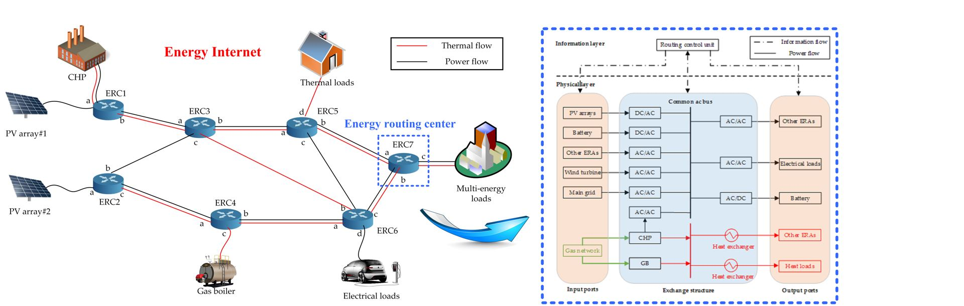
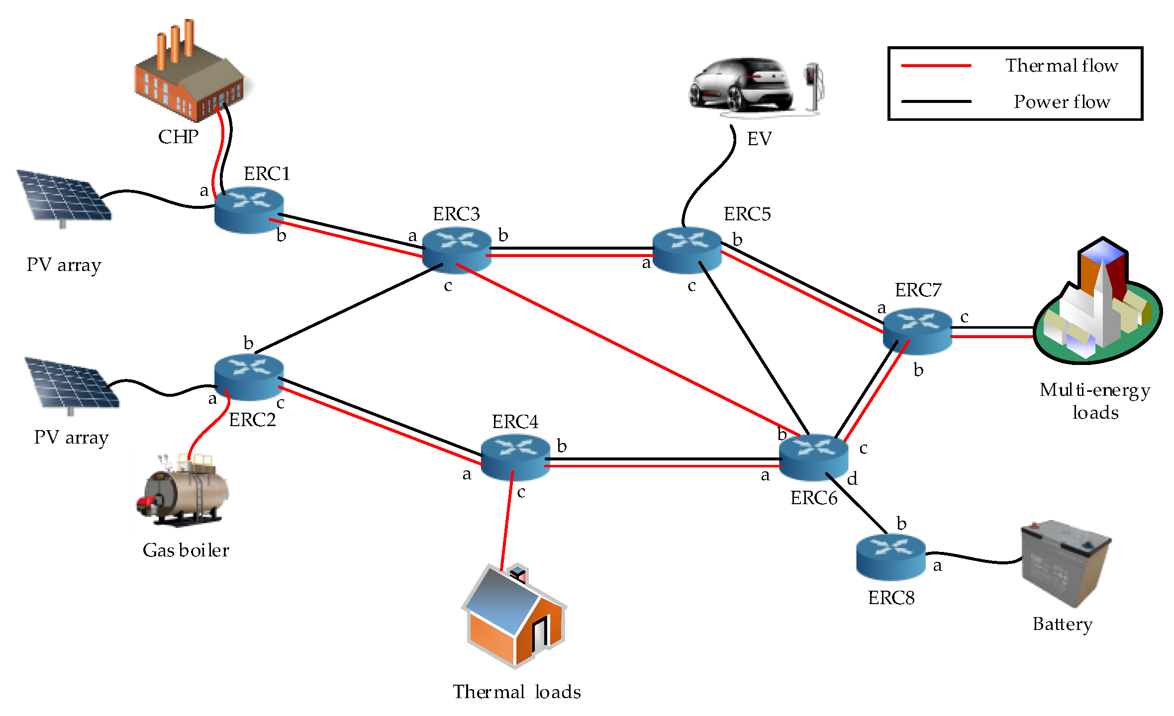
In order to form the optimal route selection strategy, weights for each connection line should be defined at first. See Figure 3 as a simple example of an EI which consists of multiple ERCs.

As can be seen in Figure 3, different ERCs are attached to each other by power connection lines and pipelines for a heat network. Since both electric energy and thermal energy are transmitted through the connection lines, operating cost, power transmission loss, and carbon emission are taken into consideration during the weights’ definition. In order to illustrate each connection line conveniently and clearly, we number the connection line between the $ith$ ERC and the $jth$ ERC as $l_{i-j}$.

3.1.1. Operating Cost

As for the operating cost, we mainly consider the operating cost of the GB and combined heat and gas, which can be defined as Equations (1) and (2), respectively:

$$C_{GB}^O={\displaystyle \sum _{i=1}^{N_{GB}}\left(a_i\times H_{GBi}^2+b_i\times H_{GBi}+c_i\right)},$$

(1)

$$C_{{}_{CHP}}^O={\displaystyle \sum _{i=1}^{N_{CHP}}\left(\begin{array}{l}{a}_i\times P_{CHPi}^2+b_i\times P_{CHPi}+c_i+d_i\times H_{CHPi}^2\\ +e_i\times H_{CHPi}+f_i\times H_{CHPi}\times P_{CHPi}\end{array}\right)},$$

(2)

where $H_{GB}$ and $H_{CHP}$ are the heat produced by gas boiler and combined heat and gas, respectively, $P_{CHP}$ is the electrical power produced by CHP.

As for renewable energy resources such as photovoltaic and wind turbine, regardless of installation cost, the operating cost of renewable energy resources can be defined as follows:

$$C_{RES}^0=p{r}_{RES}{P}_{RES}.$$

(3)

where $p{r}_{RES}$ is the operating cost per kilowatt, and $P_{RES}$ is the output power of renewable energy sources. As photovoltaic is the renewable energy resource used in this paper, the operating cost of PV is $p{r}_{RES}=0.7\mathrm{yuan}/\mathrm{kWh}$.

According to Equations (1)–(3), the operating cost function can be defined as:

$$C_{cost}^O=k_1{C}_{GB}^O+k_2{C}_{CHP}^O+k_3{C}_{RES}^O.$$

(4)

where $k_1$,$k_2$, and $k_3$ are parameters to balance the order of magnitude among operating costs.

Under general conditions, the main grid is used as a supplementary device. However, when the whole system is under an extremely heavy load, the total output power of devices in the system fails to meet the load demand of users, and electricity has to be purchased from the main grid. Therefore, the cost of buying electricity should be added to the cost function. The electricity purchasing cost can be defined as:

$$C_{grid}^O=P_{grid}\times bi{d}_{grid}.$$

(5)

where $P_{grid}$ is the power purchased from the main grid, and $bi{d}_{grid}$ is the electricity price.

Thus, the cost function of a multi-energy system can be rewritten as:

$$C_{cost}^O=k_1{C}_{GB}^O+k_2{C}_{CHP}^O+k_3{C}_{grid}^O.$$

(6)

3.1.2. Power Loss

Due to the resistance of connection lines, power transmission loss should also be taken into consideration. Power transmission loss on $l_{i-j}$ is defined as follows:

$$C_{i-j}^{Loss}=\frac{P_{i-j}^2}{V_{i-j}^2}{R}_{i-j},$$

(7)

where $P_{i-j}$,$V_{i-j}$ and $R_{i-j}$ are the transmission power, voltage level, and resistance of the connection line $l_{i-j}$. However, as $P_{i-j}$ is hard to control, the paper regulates the voltage of the connection port to determine the transmission power according to the equation as follows:

$$\Delta V_{i-j}=\frac{P_{i-j}{R}_{i-j}+Q_{i-j}{X}_{i-j}}{V_N},$$

(8)

where $Q_{i-j}$ and $X_{i-j}$ are the reactive power and reactance. As for transmission line $R\gg X$, thus the power transmission loss can be roughly defined as:

$$C_{i-j}^{Loss}=\frac{\Delta V_{i-j}^2}{R_{i-j}}=\frac{{\left(V_{ix}-V_{jy}\right)}^2}{R_{i-j}},$$

(9)

where $V_{ix}$ and $V_{jy}$ are the voltages of two ends of the connection line.

3.1.3. Environmental Cost

In order to make the energy system more environmentally friendly, pollution during the energy production process is considered simultaneously. In this paper, as natural gas is burned to supply heat, pollution mainly refers to greenhouse gases emissions such as $C{O}_2$ and $N{O}_x$. Thus, the environmental cost can be depicted as:

$$C_{GB}^E={\displaystyle \sum _{j=1}^m\left(d_{ej}{v}_{ej}{\displaystyle \sum _{i=1}^{N_{GB}}{H}_{GBi}}\right)},$$

(10)

$$C_{CHP}^E={\displaystyle \sum _{j=1}^m\left(d_{ej}{v}_{ej}{\displaystyle \sum _{i=1}^{N_{CHP}}\frac{P_{CHPi}+H_{CHPi}}{4}}\right)},$$

(11)

where $d_{ej}$ and $v_{ej}$ are emission intensity and environmental value, respectively. According to the equations above, the environmental cost function can be defined as follows:

$$C_{cost}^E=k_4{C}_{GB}^E+k_5{C}_{CHP}^E.$$

(12)

where $k_4$ and $k_5$ are parameters to balance the order of magnitude between two environmental costs.

When considering the emission cost of the main grid, coal is considered as the main fuel of the main grid, thus the environmental cost of the main grid is depicted as:

$$C_{grid}^E={\displaystyle \sum _{j=1}^m{d}_{ej}{v}_{ej}{P}_{grid}}.$$

(13)

The environmental cost function can be rewritten as:

$$C_{cost}^E=k_4{C}_{GB}^E+k_5{C}_{CHP}^E+k_6{C}_{grid}^E.$$

(14)

Emission intensities for different devices are shown in

Table 1. Emission intensities of different devices.

Types of Greenhouse Gases	$\mathbf{Emission}\mathbf{Intensity}{\mathit{d}}_{\mathit{e}\mathit{j}}\left(\mathbf{kg}/\mathbf{MW}·\mathbf{h}\right)$
	CHP	GB	Grid
$C{O}_2$	623.0000	742.6000	643.8900
$N{O}_x$	2.8800	0.2556	2.8800

as below:

In

Table 2. Environmental values of different greenhouse gases.

Types of Greenhouse Gases	$\mathbf{Environmental}\mathbf{Value}{\mathit{v}}_{\mathit{e}\mathit{j}}\left(\mathbf{yuan}/\mathbf{kg}\right)$
$C{O}_2$	0.044
$N{O}_x$	8.000

, environmental values of different greenhouse gases are given as follows:

3.2. Weights Definition of Connection Lines

During the process of energy transfer and conversion, the efficiencies of energy routing ports are different. Therefore, to some extent, the conversion efficiency affects the energy output of source, which affects the operation and environmental costs and line loss of the system as a consequence. Thus, the efficiencies of ports should be taken into account in the process of weights’ definition of connection lines.

In this paper, the weight of a connection line is composed of two parts, one part consists of operating cost, environmental cost, and conversion efficiency, while the other part contains energy loss on the connection line. The weight $W_{1,i-j}$ is defined as follows:

$$W_{1,i-j}=\left(1-{\eta }_{ix}^P\right)C_{cost}^O+\left(1-{\eta }_{ix}^H\right)C_{\cos t}^E,$$

(15)

where $x$ stands for the numbers of output ports such as $a,b,c,\cdots$. $i$ represents the number of the ERC, thus ${\eta }_{ix}^P$ and ${\eta }_{ix}^H$ means the electrical and thermal conversion efficiency of the $xth$ ports in the $ith$ ERC, respectively. According to Equation (15), the connection line $l_{i-j}$ is given a smaller weight when it is connected to a port with higher conversion efficiency.

The weight $W_{2,i-j}$ is defined as follows:

$$W_{2,i-j}=C_{i-j}^{loss}.$$

(16)

According to Equations (15) and (16), the weight of $l_{i-j}$ can be depicted as:

$$W_{i-j}=m_1{W}_{1,i-j}+m_2{W}_{2,i-j},$$

(17)

where $m_1$ and $m_2$ are parameters to balance the order of magnitude between $W_{1,i-j}$ and $W_{2,i-j}$.

To summarize, the weight of a connection line reflects its energy transmission efficiency. The larger the weight is, the more energy is wasted during the transmission process. Thus, in order to schedule an optimal energy routing path with lower power loss and less operating and environmental cost, a path with a smaller weight is preferred.

3.3. Constraints

3.3.1. Electrical Power and Thermal Power Constraints

As for the optimal energy routing path design, there are some constraints that should be satisfied. Firstly, the balance equation between energy users and energy suppliers should be satisfied as follows:

$${\displaystyle \sum _{i=1}^{N_{CHP}}{P}_{CHPi}{\eta }_{ix}}+{\displaystyle \sum _{i=1}^{N_{PV}}{P}_{PVi}{\eta }_{ix}}+P_{Grid}{\eta }_{ix}+\left(P_{ch}-P_{dis}\right){\eta }_{ix}-{\displaystyle \sum C_{i-j}^{loss}}=P_{load},$$

(18)

where $P_{ch}$ and $P_{dis}$ are charging and discharging power of battery. What is worth mentioning, as the main grid is used as a supplementary device in the proposed system, the value of $P_{Grid}$ is zero under normal condition.

$${\displaystyle \sum _{i=1}^{N_{CHP}}{H}_{CHPi}{\eta }_{ix}}+{\displaystyle \sum _{i=1}^{N_{GB}}{H}_{GBi}}=H_{load},$$

(19)

In addition to equality constraints, considering the capacity and the upper and lower bound of the device, some inequality constraints must be satisfied at the same time.

$$H_{i-j}^{\min }\le H_{i-j}\le H_{i-j}^{\max },$$

(20)

$$0\le P_{PVi}\le P_{PVi}^{\max },$$

(21)

$$0\le P_{chi}\le P_{chi}^{\max },$$

(22)

$$0\le P_{disi}\le P_{disi}^{\max },$$

(23)

$$P_{CHPi}^{\min }\le P_{CHPi}\le P_{CHPi}^{\max },$$

(24)

$$H_{CHPi}^{\min }\le H_{CHPi}\le H_{CHPi}^{\max },$$

(25)

$$0\le H_{GBi}\le H_{GBi}^{\max },$$

(26)

$$E_{bati}^{\min }\le E_{bati}\le E_{bati}^{\max },$$

(27)

where $P_{i-j}^{\max }$, $P_{PVi}^{\max }$, $P_{chi}^{\max }$, $P_{disi}^{\max }$, $P_{CHPi}^{\max }$, $H_{i-j}^{\max }$, $H_{CHPi}^{\max }$ and $H_{GBi}^{\max }$ are the upper limits of the output power of devices, while those with the superscript “min” are the lower limits of the output power of devices. $E_{bati}$ stands for the capacity of the $ith$ battery. What is worth mentioning, for the sake of security reasons and prolonging the life length of the battery, the battery is partially discharged. Therefore, the lower limit of battery is restricted to 20% of its full capacity.

3.3.2. Security Constraints

As for each connection port, the voltage deviation should be restricted to a certain range to protect the inner devices and ensure the security operation of the whole system. Therefore, the security constrains can be expressed as:

$$-7\%\le \frac{V_{ix}-V_N}{V_N}\times 100\%\le +7\%,$$

(28)

According to the security restrictions above, by regulating the voltage of each port, the power transmission on each connection line is determined at the same time.

4. Reinforcement Learning Combined with ANN

Reinforcement learning is a main class of machine learning methods which attracts attention from many scholars. Reinforcement learning agent forms an optimal policy through a series of trial-and-error processes with its environment. At each step, the learning agent interacts with the environment to obtain a current state and then selects a random action from its action set with a certain probability. After taking an action, the learning agent transform transits its state to the successive state and receives a reward according to the reward function at the same time. The reward is an important index that evaluates the effect of a certain action and influences the action policy in the future iteration potentially. The learning agent can be depicted as a tuple of $\left\{S,A,R,P\right\}$ which represents the state set, action set, immediate reward, and state transition probability, respectively.

Reinforcement learning is a valid method for solving problems which are difficult to establish in explicit environmental models. As for the multi-energy system structure proposed in Figure 3, considering the uncertainties in the energy consumptions of users and fluctuations in renewable energy generation, the relationship between energy supply and demand in each energy region changes frequently. These uncertainties lead to frequent changes in the topological relationship between load and source in multi-energy systems, therefore, it is difficult to establish an accurate model of the proposed energy system. In order to solve the optimal energy routing problem of the proposed energy system, reinforcement learning method was adopted.

4.1. Q Learning

Q-learning is one of the most popular algorithms in reinforcement learning, the Q-learning algorithm learns the value of each state–action pair, which is defined as the discounted reward over the future by taking an action from the action set. A single-step Q-learning is defined as [22]:

$$Q_{t+1}\left(s_t,a_t\right)=Q_t\left(s_t,a_t\right)+\alpha [r_{t+1}+\gamma \underset{a\in A}{\max }{Q}_t\left(s_{t+1},a\right)].$$

(29)

At each step $t$, the value of state–action pairs $\left(s_t,a_t\right)$ in the current Q table $Q_t$ is recorded. After that, the environment transits its state to $s_{t+1}$ according to the selected action $a_t\in A$ from the action space, and the learning agent receives an immediate reward $r_{t+1}$ at the same time. Additionally, in order to take the future reward into consideration, $\gamma \underset{a\in A}{\max }{Q}_t\left(s_{t+1},a\right)$ is added to the process of updating the Q table. By following the mentioned procedures, the Q table $Q_t$ is updated to $Q_{t+1}$.

$\gamma \in \left(0,1\right]$ is the discount factor which reflects the degree of importance of future rewards, the larger the discount factor is, the learning agent pays more attention to the reward received in the future. $\alpha \in \left(0,1\right]$ is the learning rate which has a significant effect on the learning speed, a large learning rate makes the learning agent learn faster.

4.2. Q Learning Combined with ANN

The traditional Q learning method uses the Q table to store the corresponding value of each state–action pair. However, the state space gets larger when the structure of the energy system is complex, and it may occupy a considerable space to store the Q table. In order to alleviate computational burdens and improve the efficiency of the algorithm, an artificial neural network is combined with a Q learning algorithm.

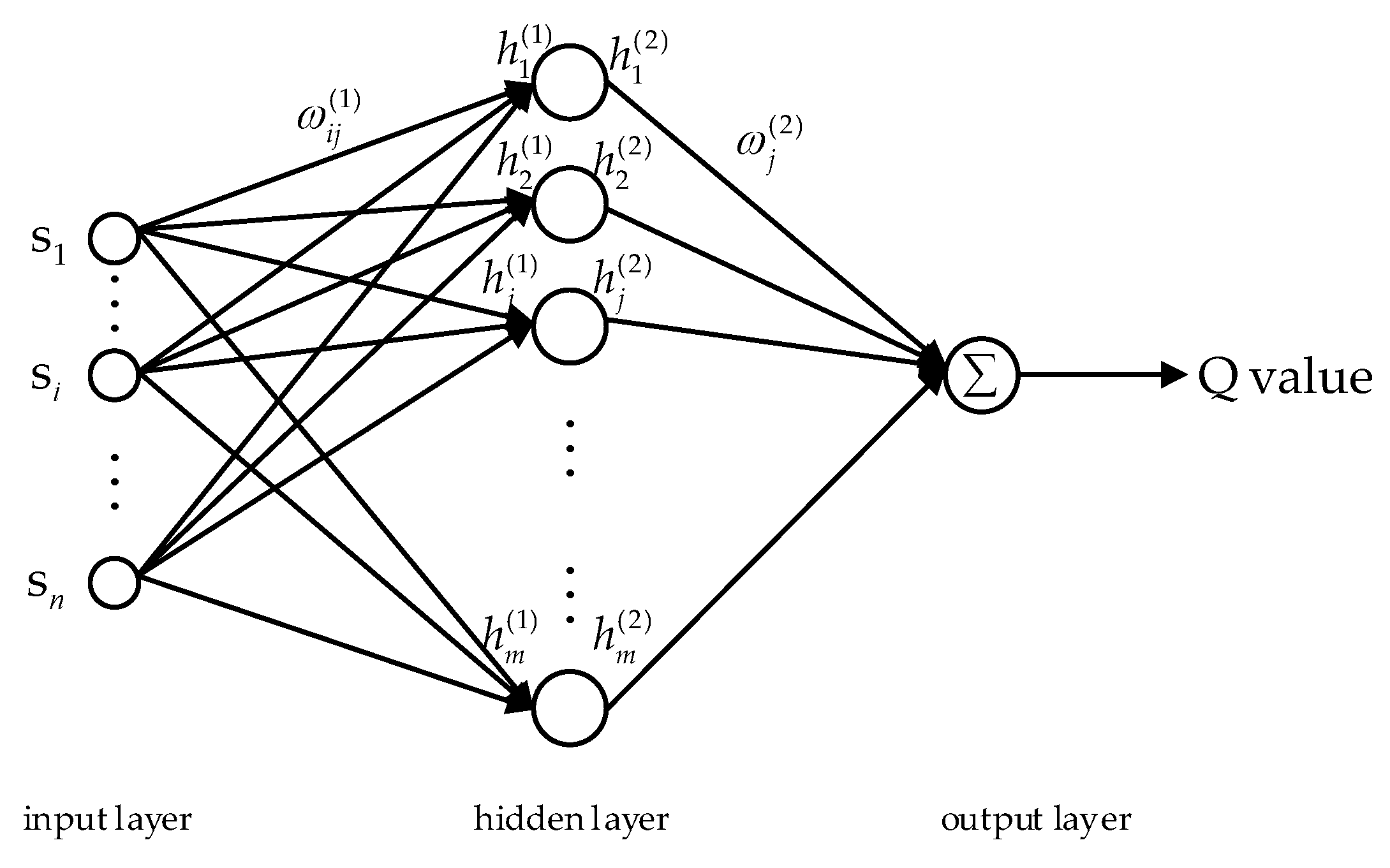
In this section ANN is combined with Q learning, a multi-layer neural network is adopted to approximate the Q value of each action. The diagram of a multi-layer neural network is proposed in Figure 4.

As shown in Figure 4, the input of the neural network is the state of the Q learning state space. Thus, the value of the state–action pair can be expressed as:

$$Q={\displaystyle \sum _{j=1}^m{\omega }_j^{(2)}{h}_j^{(2)}},$$

(30)

where $m$ is the node number of the proposed ANN, $h_j^{(2)}$ is the output of the $jth$ node, ${\omega }_j^{(2)}$ is the connection weight between the output layer and hidden layer. What is more, $h_j^{(2)}$ can be defined by the sigmoid function as:

$$h_j^{(2)}=\frac{1}{1-e^{-h_j^{(1)}}},$$

(31)

$$h_j^{(1)}={\displaystyle \sum _{i=1}^n{s}_i{\omega }_{ij}^{(1)}},$$

(32)

where $h_j^{(1)}$ is the input of the hidden layer, ${\omega }_{ij}^{(1)}$ is the connection weight between the input layer and the hidden layer.

Therefore, the connection weights of the ANN can be updated by gradient descendent according to the updating strategy of the single-step Q learning:

$${\omega }_{ij,t+1}^{(1)}={\omega }_{ij,t}^{(1)}+\alpha [r_{t+1}+\gamma \underset{a\in A}{\max }{Q}_t\left(s_{t+1},a\right)-Q_t]\frac{\partial Q_t}{\partial {\omega }_{ij,t}^{(1)}},$$

(33)

$${\omega }_{j,t+1}^{(2)}={\omega }_{j,t}^{(3)}+\alpha [r_{t+1}+\gamma \underset{a\in A}{\max }{Q}_t\left(s_{t+1},a\right)-Q_t]\frac{\partial Q_t}{\partial {\omega }_{j,t}^{(2)}},$$

(34)

where $\frac{\partial Q_t}{\partial {\omega }_{ij,t}^{(1)}}$ and $\frac{\partial Q_t}{\partial {\omega }_{j,t}^{(2)}}$ are as follows:

$$\frac{\partial Q_t}{\partial {\omega }_{ij,t}^{(1)}}={\omega }_{j,t}^{(2)}{s}_t{h}_{j,t}^{(2)}\left(1-h_{j,t}^{(2)}\right),$$

(35)

$$\frac{\partial Q_t}{\partial {\omega }_{j,t}^{(2)}}=h_{j,t}^{(2)}.$$

(36)

4.3. Q learning Combined with ANN Application in Energy Routing Design

In order to apply the proposed algorithm to energy routing design, the state space $S$, action space $A$, immediate reward $r$, and action selection policy is defined.

4.3.1. State Space

According to the structure proposed in Figure 1, an energy routing center receives energy from other ERCs if it fails to meet its users’ demands. The difference between its supply and demand can be expressed as $P_{load}$ and $H_{load}$. The state space of Q learning can be depicted as follows:

$$S=\{P_{load},H_{load}\},$$

(37)

where $P_{load}$ and $H_{load}$ are the electrical load and thermal load, respectively.

An electrical load–thermal load pair is sufficient to represent the state, every time the learning system obtains an electrical load–thermal load pair, an action will be taken to meet the load demand.

4.3.2. Action Space

According to the structure proposed in Figure 1, an energy routing center provides its redundant energy to other ERCs if necessary. The action space of Q learning can be depicted as follows:

$$A=\{P_{PV},V_{ix},P_{CHP},P_{bat},P_{grid},H_{GB},H_{CHP},H_{i-j}\},$$

(38)

where, $P_{CHP}$, $P_{bat}$ and $P_{grid}$ are the output electrical power of photovoltaic, CHP, battery, and main grid, respectively. $H_{GB}$ and $H_{CHP}$ are the output heat of GB and CHP. $P_{i-j}$ and $H_{i-j}$ are the electrical power and thermal power transmitted on connection lines. $V_{ix}$ is the voltage of the ports which are connected to the connection line.

4.3.3. Reward Function

In Section 3, the operating cost, environmental cost, and power losses are integrated and converted into the weights of the connection lines. A routing path with smaller weights is preferred in this paper, thus when the power is transmitted through such a path, the learning agent should receive a larger immediate reward. Therefore, the reward function is defined as follows:

$$r=\{\begin{array}{l}\frac{1}{W_{i-j}},\mathrm{within}\mathrm{limits}\\ 0,\mathrm{beyond}\mathrm{limits}\end{array}.$$

(39)

Considering the transmission capability of connection lines and secure operation of the energy system, upper limits should be satisfied. If the power transmitted is beyond the upper bound, the immediate reward will decrease to zero.

4.3.4. Action Selection Policy

In order to encourage the exploitation of the learning algorithm, an action selection policy is proposed as follows:

$$p\left(s,a_i\right)=\frac{e^{Q\left(s,a_i\right)/\tau }}{{\displaystyle {\sum }_{a_i}{e}^{Q\left(s,a_i\right)/\tau }}},$$

(40)

where $\tau$ is a parameter which influences the exploitation process. A larger parameter increases the randomness of the exploitation, vice versa. In this paper, the initial value of the parameter is large and it decreases after a period of iteration.

5. Simulations

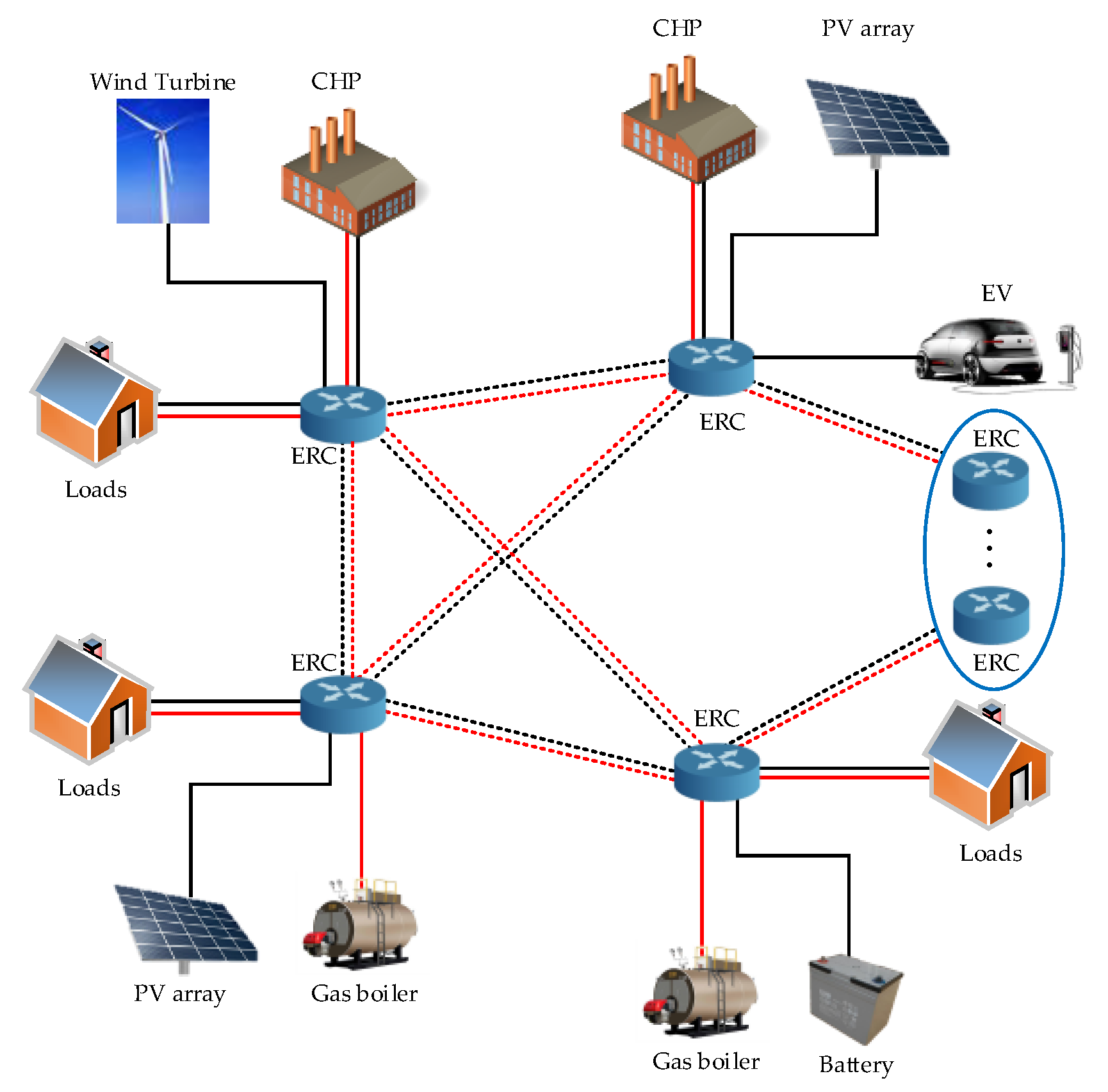
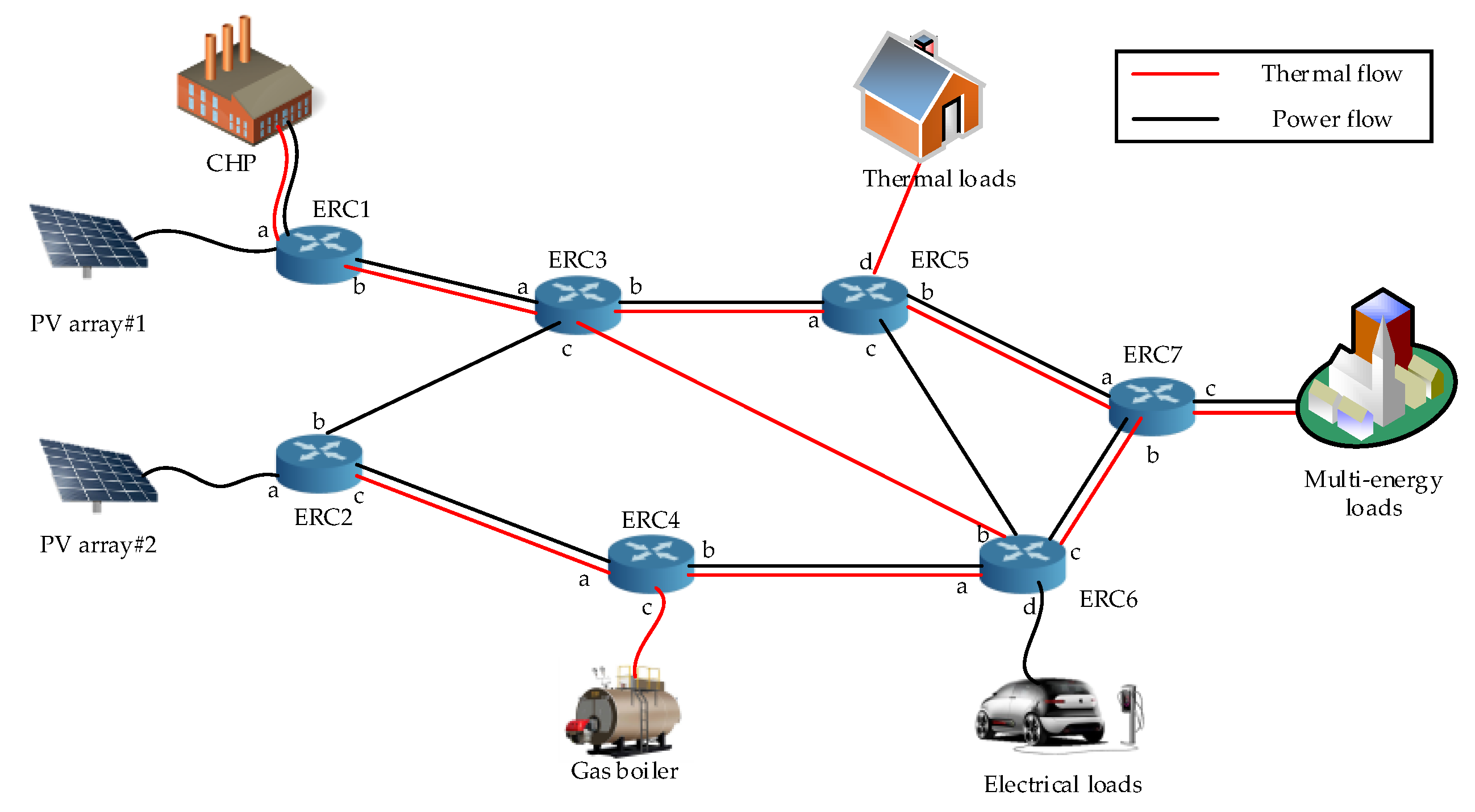
On the basis of the supply and demand relationship of each energy region, the topology of the EI with multiple ERCs can be transformed into Figure 5. In this case, multiple types of energy are integrated and multi-energy networks with different physical connection structures are connected through ERCs. Energy regions connected with ERCs in this case have diversified energy supply capacities and energy demands, and they possess the ability of supplying energy through ERCs according to their inner supply–demand relationship.

As can be seen in Figure 5, the proposed energy system includes seven energy regions which are connected through ERCs. Energy regions connected with ERC1, ERC2, and ERC4 produce excessive energy over users’ demands which are able to act as energy suppliers for other regions. At the same time, due to the excessive energy demands, energy regions connected with ERC5, ERC6, and ERC7 requires extra energy from the energy internet. Considering the output power fluctuations of renewable energy sources and the variations of user demands, an energy routing design for both electrical power and thermal power can be obtained by using the proposed algorithm in MATLAB.

In order to design the energy routing path, the efficiencies of ports in the related routing centers are proposed in

Table 3. Electric conversion efficiency of each energy routing port.

Routing Center	Port	$\mathbf{Efficiency}{\mathit{\eta }}_{\mathit{i}\mathit{x}}^{\mathit{P}}$	$\mathbf{Efficiency}{\mathit{\eta }}_{\mathit{i}\mathit{x}}^{\mathit{H}}$
ERC1	a	1	1
	b	0.97	0.98
ERC2	a	1	-
	b	0.95	-
	c	0.95	-
ERC3	a	1	1
	b	0.97	0.99
	c	0.95	0.98
ERC4	a	1	1
	b	0.97	0.98
	c	-	1
ERC5	a	1	1
	b	0.95	0.97
	c	0.97	-
	d	-	0.98
ERC6	a	1	1
	b	0.97	1
	c	0.97	0.98
	d	0.98	-
ERC7	a	1	1
	b	1	1
	c	1	1

.

To calculate the power losses on the connection lines, values of resistances and upper limits of power transfer are provided in

Table 4. Resistances and upper limits of power transfer of connection lines.

Line	$\mathbf{Resistance}{\mathit{R}}_{\mathit{i}-\mathit{j}}\left(\mathbf{\Omega }\right)$	$\mathbf{Upper}\mathbf{Limits}{\mathit{P}}_{\mathit{i}-\mathit{j}}\left(\mathbf{kW}\right)$	$\mathbf{Upper}\mathbf{Limits}{\mathit{H}}_{\mathit{i}-\mathit{j}}\left(\mathbf{kW}\right)$
$l_{1-3}$	0.24	58.33	50
$l_{2-3}$	0.37	37.84	-
$l_{2-4}$	0.54	25.93	-
$l_{3-5}$	0.41	34.15	80
$l_{3-6}$	-	-	35
$l_{4-6}$	0.65	21.54	80
$l_{5-6}$	0.45	31.11	-
$l_{5-7}$	0.55	25.45	60
$l_{6-7}$	0.60	23.33	70

as follows:

The parameter of operating cost is proposed in

Table 5. Parameters of operating cost.

Device	Parameters
	$\mathit{a}$	$\mathit{b}$	$\mathit{c}$	$\mathit{d}$	$\mathit{e}$	$\mathit{f}$
Gas boiler (GB)	0.038	2.011	65	-	-	-
Combined heat and power (CHP)	0.0065	1.21	2	0.003	4	0.61

The capacities of devices in the proposed energy system are shown in

Table 6. Capacities of devices.

Device	Lower Bound (kW)	Upper Bound (kW)
GB	0	100
CHP (electric)	0	60
CHP (thermal)	0	80
Photovoltaic (PV)#1	0	25
PV#2	0	25

as follows:

Learning rate and discount factor are two significant parameters which influence the performance of the learning process. A large learning rate shortens the whole learning process by accelerating its transformation towards the newly estimated value. However, it brings risks to the convergence of the algorithm. An excessive large learning rate slows down the convergence process and even results in divergence. On the contrary, a small learning rate ensures the stability of the convergence process but prolongs the learning process evidently. In this paper, the selected learning rate ensures the performance of both the learning speed and convergence process.

As for the problem researched in this paper of which adjacent states correlated, the action of the former state significantly affects the actions of the following state, a small discount factor may be harmful. By using a small discount factor, the algorithm risks trapping the local minimum and fails to get the optimal solution. Therefore, a larger discount factor was selected in this paper. The Q learning parameters were selected in

Table 7. Selection of Q learning parameters.

Learning Parameters	Value
Discounted factor	0.7
Learning rate	0.9

as follows:

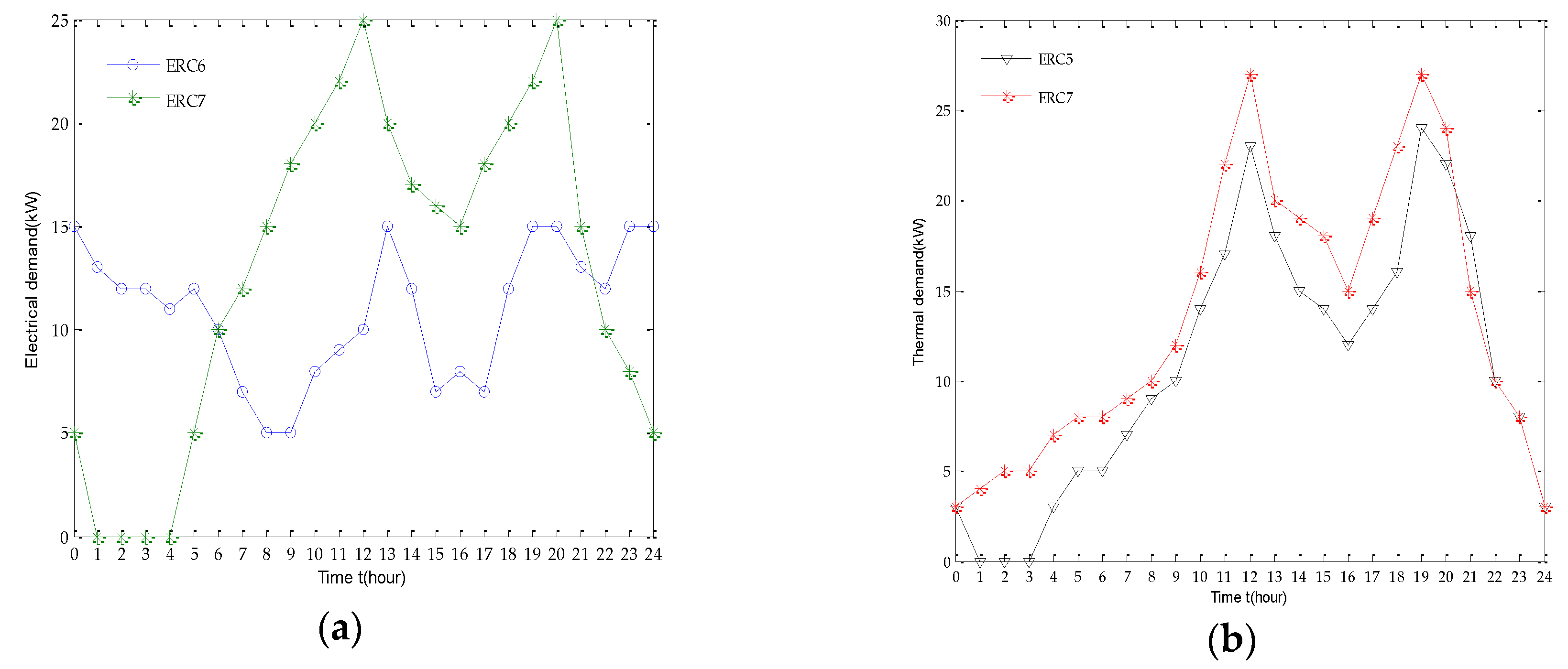
According to the structure proposed in Figure 5, the electrical power demands and heat demands are shown in Figure 6.

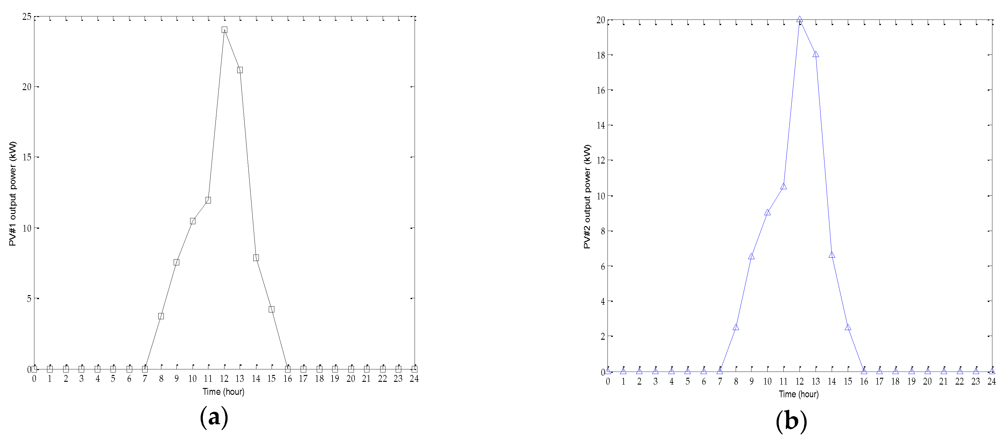
The output of photovoltaic in ERC1 and ERC2 can be depicted in Figure 7 as follows:

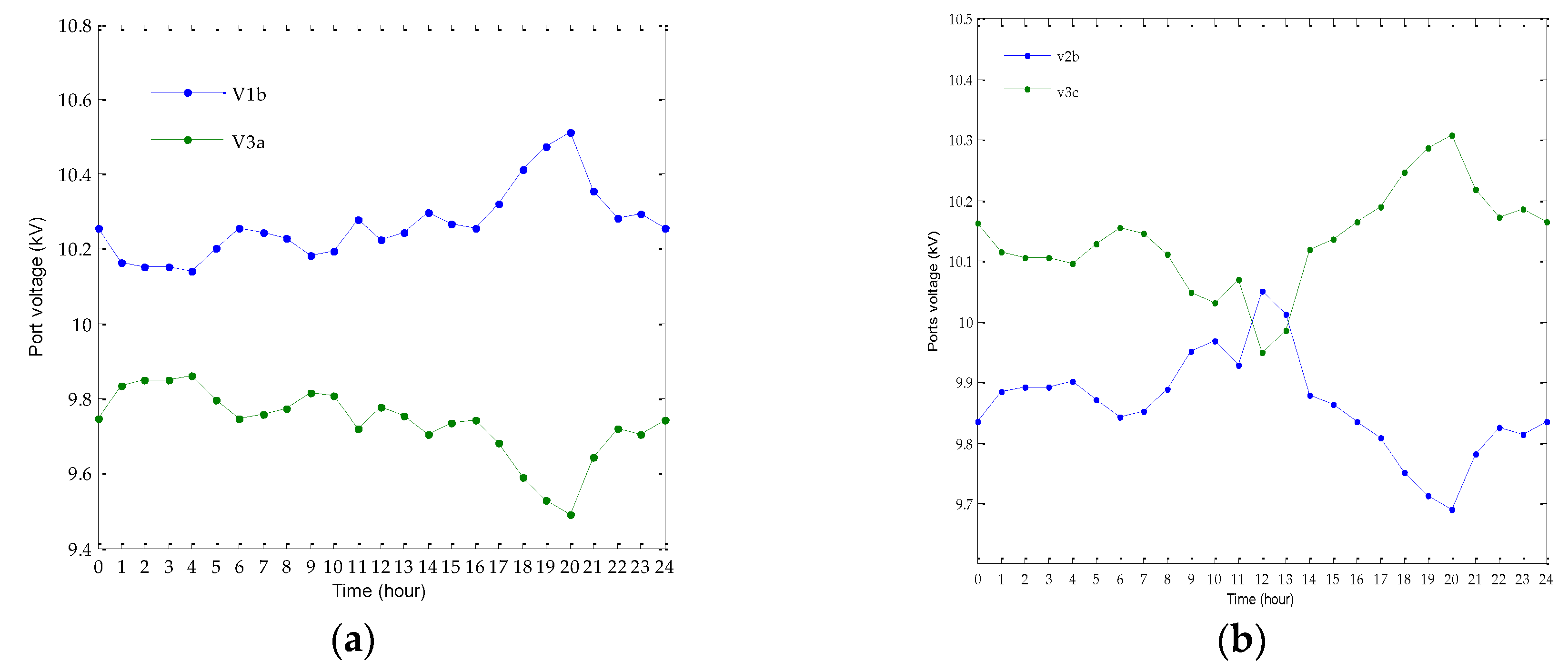
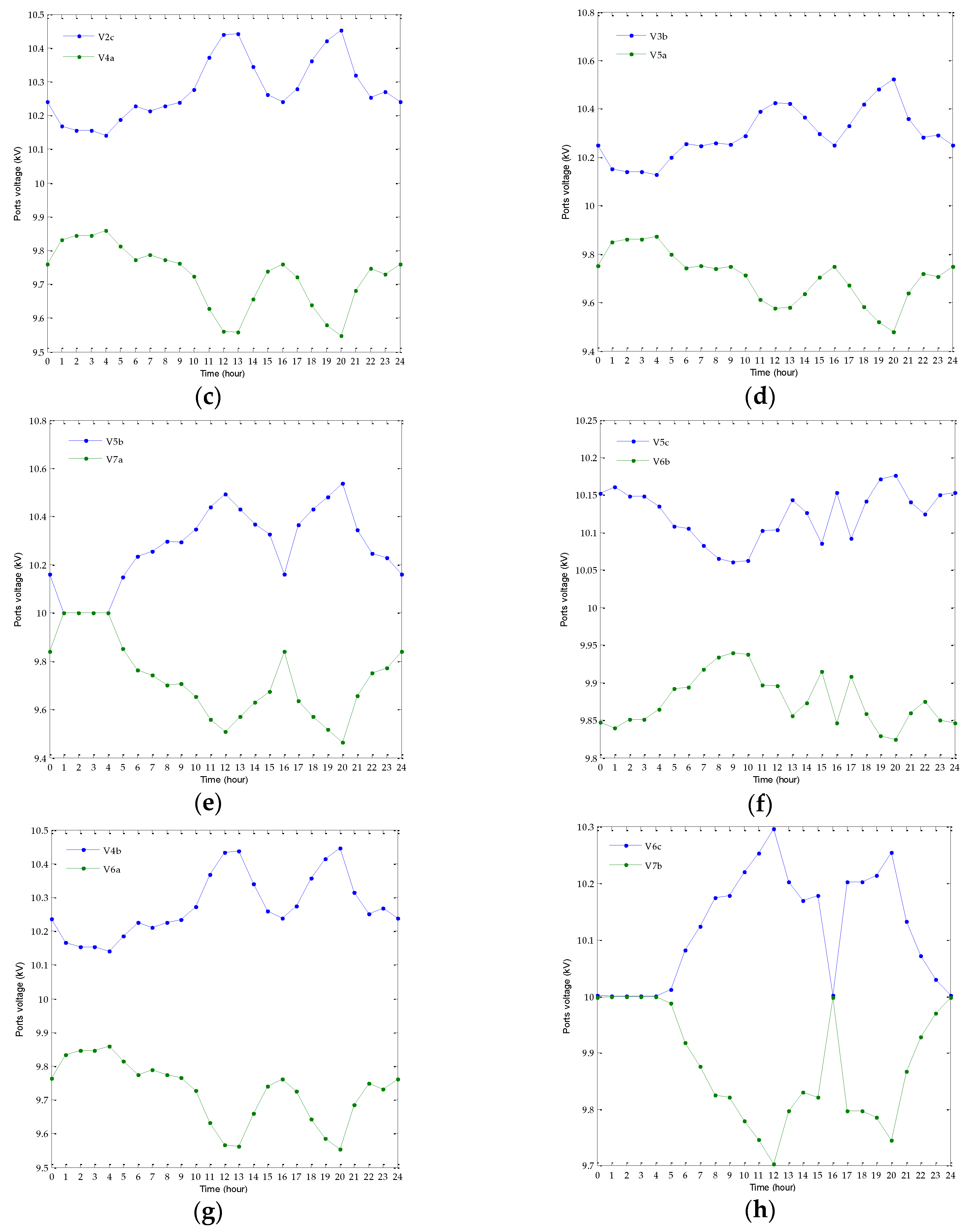
The energy routing design for both electrical power and thermal power can be obtained by using the proposed algorithm. The voltages of the ports connected with connection lines can be obtained which is illustrated in Figure 8.

As shown in Figure 8, the voltage deviation on a transmission line reflects the amount of electrical power that can be transmitted through the line. More power can be transmitted under a larger voltage difference between two ports. 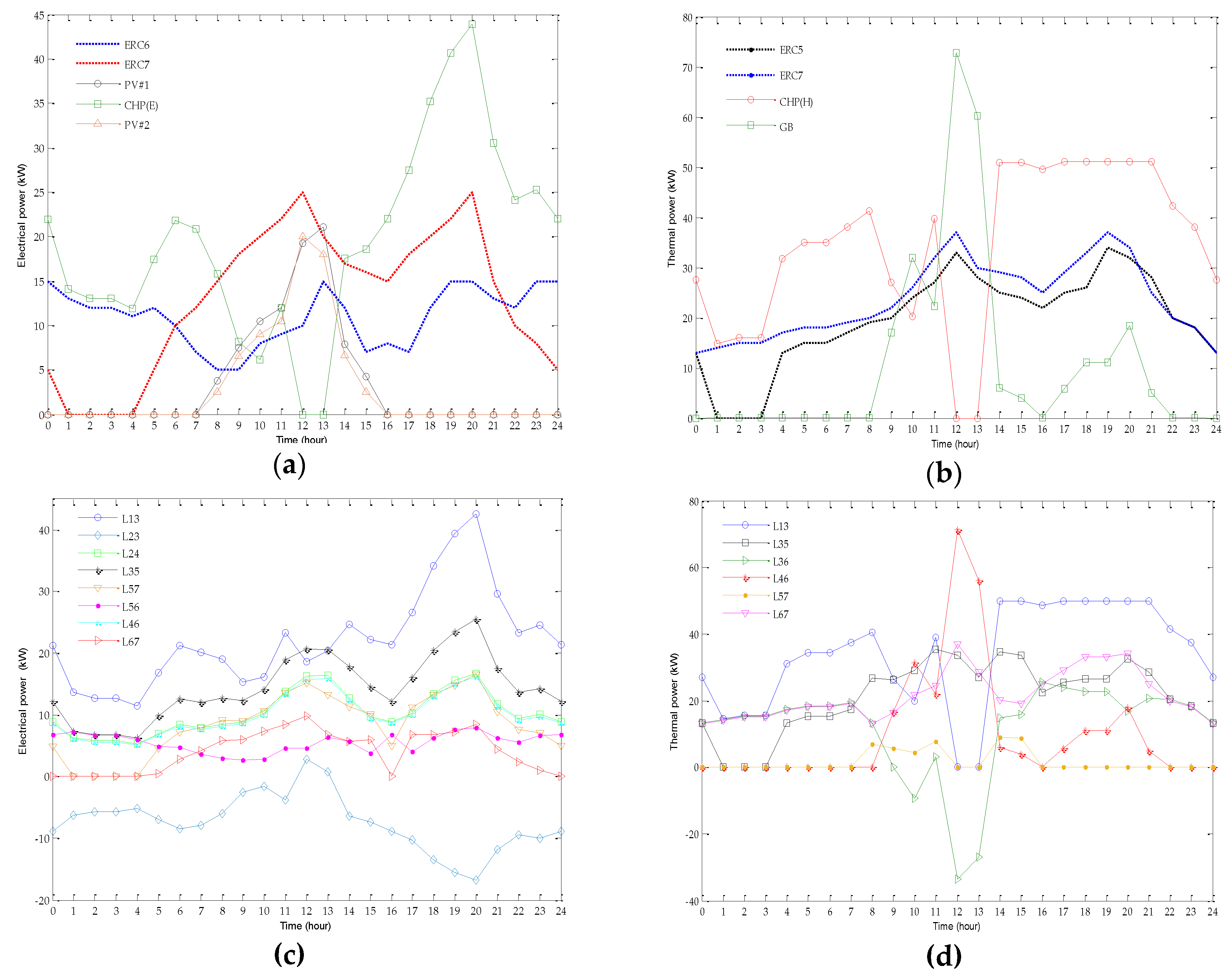According to Figure 8, the voltage of each ports can be obtained, therefore the power transmitting on each connection line can be calculated according to Equation (9) and the energy-management-based energy routing strategy is shown in Figure 9.

As shown in Figure 9a, the electrical power outputs of different devices are illustrated and the electrical demands of ERC6 and ERC7 are plotted by dotted lines. During 0:00–8:00 and 16:00–24:00, the output power of PV arrays is zero, and CHP is used to produce electricity. The output power of PV increases over time; therefore, from 9:00–15:00, renewable energy is given priority in supplying electricity to meet users’ demand due to its low operating and environmental costs. From 12:00–14:00, the total output power of two PV arrays is able to meet the whole electrical power demand, consequently, CHP is not involved in the process of supplying energy. While at the other times in a day, due to environmental factors, the output of PV fails to meet the total electrical power demand. Therefore, CHP is used to compensate the difference between supply and demand.

As can be seen in Figure 9b, CHP and GB are used to supply thermal power to users of other energy regions. In most hours of a day, only CHP is used to produce heat. What is worthy of mentioning, in order to ensure the efficient operation of CHP, the ratio between its output electrical power and thermal power is limited to a certain range which is defined to be 100–300% in this paper. During 10:00–12:00, the increase of PV output leads to a reduction of electrical power from CHP. As a consequence, the thermal output of CHP is restricted, and GB is forced to generate more heat to satisfy users’ demands. From 12:00–14:00, CHP is not involved in the energy supplying process, and GB is used to transmit heat to users.

In Figure 9c,d, energy routing paths for different hours are shown, the negative power means that the direction of power flow is contradicted with the prescribed direction. As for electrical power transmission, ERC1 tends to transmit its electrical power on the routing path through ERC3 and ERC5 due to its high conversion efficiency which reduces the operating cost and environmental cost of CHP. However, a large amount of electrical power transmission on connection lines leads to a significant increase in power losses. In order to seek the balance between power losses and operating cost, electrical power is also transferred through the path composed of ERC3, ERC2, and ERC4. As for thermal power transmission, in most hours in a day, heat is transmitted mainly through the path of ERC3 and ERC5 and the path with ERC3, ERC6 and ERC7to the thermal users due to their high conversion efficiency. However, from 12:00–14:00, GB is used to compensate the total demand of users, and the energy routing strategy is changed simultaneously. The thermal power is transferred through the path of ERC4, ERC6, and ERC7, and the path of ERC4, ERC6, ERC3, and ERC5 during the period.

6. Conclusions

In order to realize flexible energy conversion and power dispatch for multi-types of energy, the concept of ERC is proposed in this paper for multi-energy coupled EI. In the proposed EI, different energy regions are connected through energy routers and connection lines which allow bi-directional energy interaction. Based on the proposed structure of EI, a multi-energy management-based optimal energy routing design problem considering operating cost, environmental cost, and security operation was studied. Considering the uncertainties of users’ energy consumption and fluctuations in renewable energy generation, it is difficult to establish an accurate model of the proposed energy system. Thus, a reinforcement learning algorithm combined with an artificial neural network was adopted to formulate the optimal energy routing strategy. By using an artificial neural network-based Q learning algorithm, the optimal output of each device can be scheduled and the optimal energy routing path can be dynamically managed according to the fluctuations of renewable energy resources and users’ demand.