Modelling of Ion Transport in Electromembrane Systems: Impacts of Membrane Bulk and Surface Heterogeneity

Abstract

Artificial charged membranes, similar to the biological membranes, are self-assembled nanostructured materials constructed from macromolecules. The mutual interactions of parts of macromolecules leads to phase separation and appearance of microheterogeneities within the membrane bulk. On the other hand, these interactions also cause spontaneous microheterogeneity on the membrane surface, to which macroheterogeneous structures can be added at the stage of membrane fabrication. Membrane bulk and surface heterogeneity affect essentially the properties and membrane performance in the applications in the field of separation (water desalination, salt concentration, food processing and other), energy production (fuel cells, reverse electrodialysis), chlorine-alkaline electrolysis, medicine and other. We review the models describing ion transport in ion-exchange membranes and electromembrane systems with an emphasis on the role of micro- and macroheterogeneities in and on the membranes. Irreversible thermodynamics approach, “solution-diffusion” and “pore-flow” models, the multiphase models built within the effective-medium approach are examined as the tools for describing ion transport in the membranes. 2D and 3D models involving or not convective transport in electrodialysis cells are presented and analysed. Some examples are given when specially designed surface heterogeneity on the membrane surface results in enhancement of ion transport in intensive current electrodialysis.

1. Introduction: Heterogeneity and Multiscale Nature of Ion Transport in Membrane Systems

The main aim of this paper is to give a review of the well-established models as well as new approaches for describing the transport phenomena in charged membranes. These materials include ion-exchange (IEM), nanofiltration (NF) and reverse osmosis (RO) membranes, which are widely used in separation and energy production processes.

The peculiarity of mass transfer phenomenon is membrane systems is the multiscale character of ion and water transport, which is due to the heterogeneity at multiple scales [1]. The charged membranes are self-assembled nanostructured materials constructed from macromolecules [2]. It is remarkable that the structure and, hence, the properties of both biological and artificial membranes show considerable similarities [3,4]. The main components of the structure are amphiphilic compounds, which have both hydrophilic and hydrophobic constituents. The mutual interaction of the hydrophobic segments and the interaction of polar hydrophilic groups with aqueous medium lead to a self-organized stable structure. In particular, nanoscale hydrophilic channels which are selectively permeable to water and ions are formed within a hydrophobic matrix [5]. The size of transport channels is of a few nanometres, so that the electrical double layers (EDL) formed at the opposing pore walls overlap. Overlapping EDLs leads to an essentially higher concentration of the ions whose sign of the charge is opposite to the that of the fixed ions (the counterions) in comparison with the concentration of the ions having the same sign of the charge as the fixed ions (the co-ions).

The second scale is due to the diffusion boundary layers (DBLs) at the membrane surface formed under the action of the electric current flowing across the membrane. This scale is of the order of 100 μm. When an overlimiting current density flows, an intermediate scale determined by the thickness of the extended space charge (of the order of 1 μm) appears.

Finally, there is a scale of the order of 10 cm determined by the length of a compartment in an electrodialysis (ED) stack used in industrial process.

The processes occurring at one scale are coupled with the processes occurring at other scales. For example, selective ion transport in membrane pores causes concentration polarization, that is, formation of concentration gradients in the DBLs of bathing solution.

In this paper, we consider the transport at all the mentioned above scales and examine the possibilities of multiscale modelling. The latter is rather difficult, as such modelling needs large computer resources. We give the mathematical description of ion transport in the membranes taking into account the structure-properties relationships. Concentration polarization occurring at the scale of DBL and related surface phenomena such as water splitting along with current induced convection are described as well. Their mechanisms are analysed in close relation with the membrane surface properties. Here we focus on the role of the membrane surface heterogeneity, which has been subject to intensive attention in the literature of recent years. Effects associated with desalination of the solution in the longitudinal direction along the length of an ED compartment are also studied.

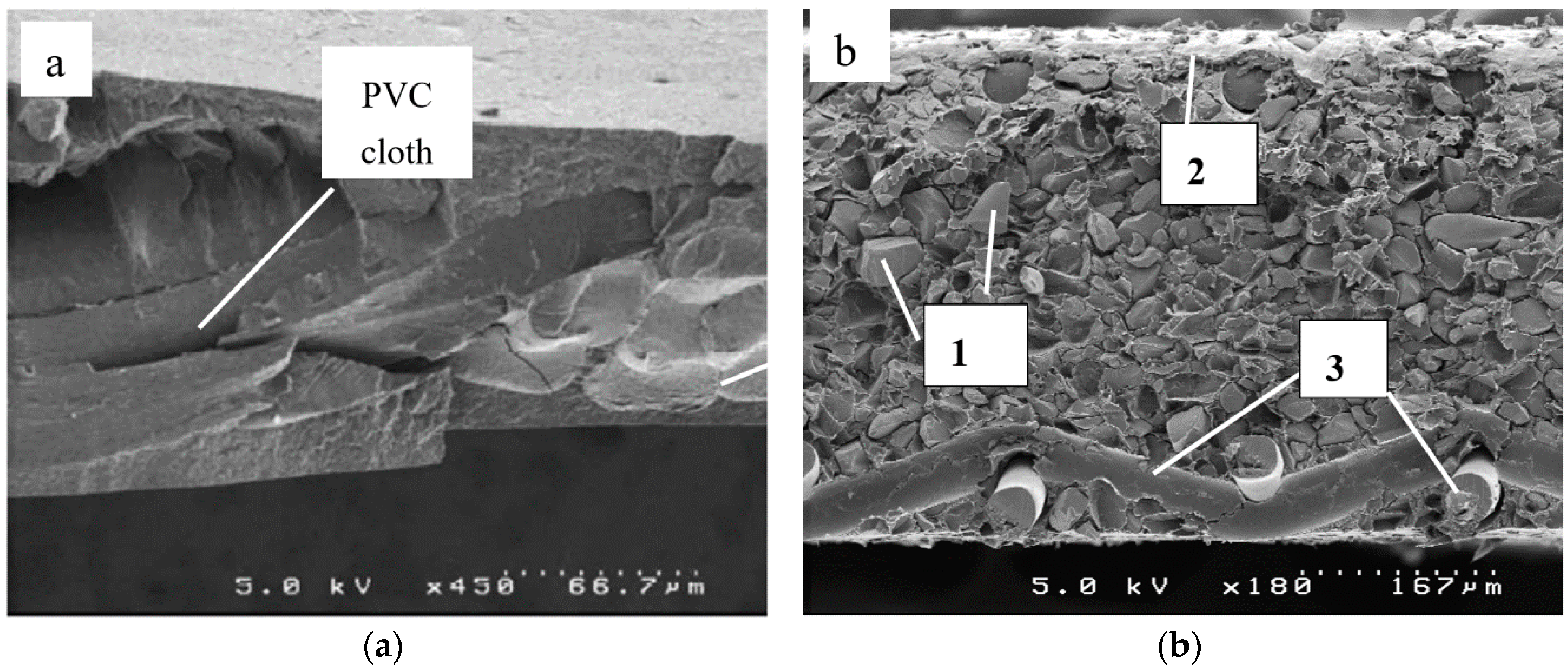
2. Structure of Ion-Exchange Membranes

Synthetic IEMs are built using flexible polymer chains with aliphatic, aromatic or perfluorinated residues, which contain functional groups such as -SO₃H, -COOH, -NH₃OH and others. Protons or ОН⁻- ions of these groups can be replaced by cations or anions, respectively, from bathing solutions.

The diversity of practical applications of membranes conditions a variety of specific requirements expected from them and, eventually, promotes the development of a wide range of membrane materials. A considerable number of membranes and membrane materials are now available [6,7,8].

Depending on the material structure and the method of preparation, IEM are usually divided into homogeneous and heterogeneous membranes. Homogeneous membranes (Figure 1a) are generally obtained by copolymerization of monomers [9] that produces homogeneous material at least at the scale of 100 nm or more, which is determined by the size of polyvinyl chloride (PVC) particles used as a non-conductive binder in the Neosepta^® membranes [10]. Heterogeneous membranes include macroparticles (with the size from 1 to 50 μm) of different polymer materials. For example, the MA-40 anion-exchange membranes (AEMs) (Shchekinoazot, Tula Region, Russia) contain particles of polystyrene crosslinked with divinylbenzene (DVB) anion-exchange resin and polyethylene used as the binder (Figure 1b). Both homogeneous and heterogeneous membranes contain reinforcing cloth (Figure 1a,b). This cloth not only plays an important role as a means to improve the mechanical properties but also causes a certain undulation of the membrane surface, which seems important for initiating electroconvection in overlimiting current regime [11].

Recently, Svoboda et al. [13] developed a specific scanning cell for the analysis of heterogeneous IEM structure by micro-computed tomography, which provides volume reconstruction of the studied material. The unique working principle of the cell allows one to scan membranes not only in their dry state but also in fully swollen state. The micro-computed tomography showed that there are profound changes in the structure of the IEM associated with their transition from the dry state into the swollen one. This study applied to the heterogeneous cation-exchange membrane (CEM) coming from Mega a.s., Česká Lípa District, Liberec Region, Czech Republic showed that swelling of the membrane is caused by the swelling of the ion-exchange resin. Its volume increased nearly three times after exposure to deionized water, while the overall membrane volume increased by 50%. If the membrane contained approximately 28%vol. of the resin in the dry state, this content increased to 52%vol. after swelling.

Micro-computed tomography not only allows one to analyse volumetric composition of the membrane bulk but also to quantify the composition of the surface. By using two different methods, Vobecka et al. [14] evaluated the fraction of the conductive area (e.g., the ion-exchange resin) on the surface of an AEM and CEM in the swollen state. The obtained results showed that the volume fraction of the conductive domains does not correspond to the surface fraction of these domains and thus the volume composition is not reflected on their surface. For example, the volume fraction of the conductive domains for the studied AEM was 0.45 and its surface fraction only 0.26. Similar results were obtained earlier by Volodina et al. [15] and other authors [16]. The reason is that during the hot pressing of heterogeneous membranes, polyethylene, which is more fluid than polystyrene, moves from the membrane bulk on the surface.

A membrane can include one or several layers. Generally, monopolar IEM have a single-layer structure [17]. Sometimes, commercial IEMs contain several layers (anisotropic membrane structure), namely, a thin skin layer and a supporting layer [18] The skin layer serves to give the membrane some special properties: antifouling resistance [19] or monovalent ion permselectivity (e.g., Neosepta monovalent ion permselective ACS and CMS membranes produced by Astom, Japan) [20,21,22] or other [23]. Bipolar membranes consist of two layers, a CEM and an AEM [6,7,24,25,26,27].

As it is mentioned above, the terms “homogeneous” and “heterogeneous” IEM are commonly used in the field of IEMs to distinguish between the membranes produced using the paste method and the membranes made via the hot pressing of powdered resins and inert binder. However, “homogeneous” membranes are not strictly speaking homogeneous. For instance, Nafion^® is a perfluorinated sulfonated ion-exchange dense polymer generally considered as homogeneous [28]. Nevertheless, when swelled in water, it contains hydrophilic pores/channels confined within a hydrophobic matrix [5]. These pores/channels provide for the transport of ion and water through a Nafion membrane. The presence of internal solution within a hydrophobic matrix allows one to speak about phase separation [5]. From this point of view, this membrane is multiphase and heterogeneous, however, this heterogeneity appears on a scale of the order of 10 nm.

The main structural feature of the functional part of IEMs (which is an ion-exchange resin in the case of heterogeneous membranes) is the hydrophobic backbone of hydrocarbon or perfluorinated chains, which antagonizes the hydrophilic character of the charged functional groups. Due to the flexibility of the polymer chains, this combination provides self-organization during the membrane formation [29]. Polymer chains form the matrix of the membrane, whereas the functional groups are aggregated in clusters. The size of the clusters is of the order of a few nanometres. Consequently, the hydrophobic components contribute to the morphological stability of the membrane. The hydrophilic domains create a system of conducting channels. When placed in an aqueous solution, hydrophilic functional groups are hydrated and the membrane swells. The size of clusters increases, conducting channels appear between them and they form a percolation system when a certain water content is reached [30]. The water content and degree of swelling depend on the external solution concentration: with increasing solution concentration water content of an IEM decreases [30,31]. When a membrane contains weakly basic functional groups, such as secondary and tertiary amino groups, there is a dependence of water content on the external solution pH [31,32,33]. The model of clusters and channels first proposed by Gierke [34] describes these main features and explains correctly the transport properties of IEMs [5,30,35]. A rather realistic presentation of two-dimensional structure of Nafion^®, which generally complies with the Gierke model, is made by Kreuer [36]. The clusters, channels, some defects of the structure, spaces between ion-exchange resin particles, the binder and the fabrics of the cloth form a system of pores in an IEMs, whose size varies from a few nm to 1–2 μm [13,37,38,39]. The investigations of the pore size distribution made using the standard contact porosimetry (Divisek et al. [40]; Berezina et al. [37] and Kononenko et al. [38,39]) and differential scanning calorimetry (DSC)-based thermoporosimetry (Bryk et al. [41]; Berezina et al. [42]; Kononenko et al. [39]) methods have shown that the homogeneous IEMs (namely, perfluorinated MF-4SK membranes (Plastpolymer, Russia) [39,41,42]), as well as Nafion-112, Nafion-115, Nafion-117 membranes [40]) do not contain macropores (the pores, whose effective radius size is larger than 100 nm), while heterogeneous membranes have such pores. It was found [37,39,42] that the pore size distribution of Russian heterogeneous MK-40 and MA-40 membranes has two maxima, the first one is at about 10 nm (which is the range of micro- and mesopores) and the second one relates to macropores with size of about 1000 nm. According to [39], the pores of the first type are situated within the ion-exchange resin particles and the pores of the second type are formed by the spaces between different membrane constituents (resin, binder, cloth).

The solution filling the clusters where the fixed functional groups are concentrated is charged. It contains mainly counterions coming from the dissociation of functional groups. The counterions being in thermal motion are attracted by the fixed charged groups, forming in this way an EDL. A pore also contains a small amount of co-ions carrying a charge of the same sign as that of the fixed ions. The co-ions are repelled from the pore by electrostatic forces; this effect is called the Donnan (co-ion) exclusion [31]. The distribution of ions within the EDL formed at inner or outer interfaces is described by the Gouy-Chapman theory, which takes into consideration both electrostatic and thermal interaction. Figure 2 schematically shows the ion distribution in the proximity of a pore wall represented as a charged plane. The concentration of counterions in the pore solution increases and that of co-ions decreases with decreasing the ratio of the pore radius to the Debye length. The latter characterizes the EDL thickness. Therefore, the less the pore radius, the higher the membrane selectivity (and the higher the membrane resistance). When the pore radius is higher than the Debye length, there is an electrically neutral solution in the pore centre.

When the water molecules are close to the functional groups, they are structured and lose to a great extent their mobility [3,5]. As a result, the relative dielectric permittivity, ε, decreases when approaching a functional group. The mobility of counterions concentrated near the functional groups is very low mainly due to strong electrostatic interaction [3,5]. The side-chains also contribute to their low mobility by encumbering the space [43]. Due to the finite size of hydrated counterions, their concentration decreases when the distance from a fixed group becomes lower than about 0.5 nm. When getting close to the pore centre, the counterion concentration decreases as well, according to the Gouy-Chapman law of ion distribution in EDL (Figure 2).

The transport properties of the central zone of a hydrophilic domain are different from those of a zone, which is close to the internal interface. The water molecules located in the centre of sufficiently large pores behave as in free solution. In particular, ε approaches the value of 81 there, as in free solution [44]; the proton transport mechanism in the pore centre is identical to that in free solution. The Grotthuss shuttling dominates over the vehicular transport (solvation diffusion): proton jumps from one H₃O+ (or H₅O₂+ or even greater) complex to a neighbouring one rather than moves within its aqueous environment-hydration shell [44]. The contribution of the vehicular transport increases with increasing the degree of water structuring, which takes place in the vicinity of the fixed charged groups. The volume fraction of bulk-like water depends on the membrane water content. Electronic structure calculations [45] show that 2–3 water molecules (n) per sulfonic acid group are needed in perfluorinated membranes (such as Nafion^®) for proton dissociation. The dissociated proton is separated from the sulfonate anion, when 6 water molecules are added in a membrane. According to Kreuer et al. [5], only when n > 14, one can speak of a two-phase system where the bulk-like water is clearly distinguishable in the pore.

Schematically, the structure of a functional part of an IEM is shown in Figure 3. It is a fragment including hydrophobic domains of the matrix, micropores (where the EDLs are overlapped) and mesopores (where the EDLs are not overlapped but occupy an essential portion of a pore). This fragment is typical for a homogeneous IEM. Heterogeneous IEMs contain also macropores (spaces between ion-exchange resin particles and reinforcing binder and tissue).

To pass from one fixed ion to a neighbouring fixed ion, a counterion has to overcome a potential barrier. The height of this barrier depends on the energy of electrostatic interactions between the hydrated counterion and the fixed ion, on the chemical interaction between this pair of ions and on the energy required to move the polymer chains to form a sufficiently large ion transport channel in the matrix. The average distance between two neighbouring fixed ions, b, depends on the exchange capacity and membrane morphology. For common membrane materials, b is in the range 0.5–1.0 nm [3]. This distance for the fixed ions in a hydrated cluster of perfluorosulfonic membranes is about 0.8 nm [3,5].

Kamcev et al. [47,48,49] propose to use the Bjerrum length as the distance from the fixed ions, which determines the boundary dividing the electrolyte solution in membrane pores into two parts whose properties are different. The Bjerrum length, λ_B, is the distance at which the electrostatic potential energy between two charges equals the thermal energy scale [50]. According to Bjerrum, if a counter-ion is closer to the fixed charge than λ_B, it is regarded as “associated”: its electrostatic interaction with the fixed ion is so great that it cannot diffuse away from the fixed charge [48]. If the distance between two ions is less than λ_B, the energy of electrostatic interaction exceeds the kinetic energy of thermal motion, which reduces the mobility of ions. Manning [51,52] proposed a model for polyelectrolyte known as the Manning condensation theory [53]. Kamcev et al. [47,48,49] have applied recently this theory to ion-exchangers. According to [49], if the distance between two fixed charges (b) is less than λ_B, counterions condense (or localize) on the polymer chain, which is a result of strong electrostatic interaction between the fixed ions and mobile counterions. When b > λ_B, counterion condensation does not occur. The value of λ_B in water is 0.71 nm, in IEMs with the IEC close to 2 meq. (g dry membrane)⁻¹] its value is 1.2–1.3 nm [49] (due to lower dielectric permittivity in IEMs). The value of b in the IEMs studied by Kamcev et al., was evaluated between 0.43 and 0.57 nm [49].

3. Irreversible Thermodynamics Approach

There are several approaches for describing ion and water transport in membranes. Some books [54,55,56,57] and reviews [58,59,60] deal with this topic. Phenomenological approach based on the irreversible thermodynamics provides a rather simple mathematical description, which, however, is not directly related to the membrane structure. This approach will be considered in this section. The structure-properties relationships may be described using other approaches, which take into account parameters of membrane structure. These approaches, considered below, involve the “solution-diffusion” and “pore-flow” models.

3.1. The Onsager Phenomenological Equations

The strength but also the weakness of the description of ion and water transport across the membranes in the framework of irreversible thermodynamics is that information about the membrane structure and transport mechanism is not used. This approach gives general relationships between fluxes and driving forces, which are valid for any type of membrane. The specificity of a given membrane is taken into account through a set of phenomenological coefficients, which cannot be found within this approach. Usually, these coefficients are determined in specially designed experiments, which is sufficient for engineering purposes. However, a more theoretical way is possible, when the transport equations of irreversible thermodynamics are completed with other equations/boundary conditions, taking into account the details of membrane structure.

At the equilibrium state, the electrochemical potential, μ_i, of any mobile species i (an ion or a molecule) is the same in every point of the membrane material. If nonzero gradients dμ_i/dx are applied, fluxes of different species appear. If the system is close to equilibrium, linear relations between the thermodynamic forces, F_j = −dμ_i/dx and resulting fluxes, J_i, can be written [56,61]:

$$J_i=-{\displaystyle \sum _j{L}_{ij}d{\mu }_j/dx}$$

(1)

where L_ij are the phenomenological conductance coefficients. In addition to the material properties, L_ij, can depend on the species concentrations, temperature and pressure but not on fluxes and forces.

It is assumed that no net transfer occurs in the direction parallel to the membrane surface, and, therefore, the value of μ_i is the same at every point of the plane normal to this direction, regardless of the phase through which the plane passes (Figure 3). dx in Equation (1) can be interpreted as a distance between two planes perpendicular to the transport axis x, the first one corresponding to the value of μ_i on the plane at the distance x, μ_i(x), the second one to μ_i(x + dx) [62,63].

Note, that Equation (1) shows that J_i depends not only on the force applied to species i, F_i but also on all forces applied to other species.

It is suitable to present the L_ij coefficients as functions of the “virtual” electroneutral solution concentration. This solution is assumed to be in local equilibrium with a small volume of the membrane. The notion of virtual solution was first introduced by Kedem and Katchalsky, who named it “corresponding solution” [64]. This solution may be physically present in the central zone of meso- and macropores (where the pore radius is higher than the Debye length) (Figure 3); if not (the EDLs at the opposite walls of the pore are overlapped), it may be considered as a hypothetical solution. Since usually local equilibrium at external membrane interfaces takes place, the virtual solution is identical to the external bathing solution at each membrane side.

The electrochemical potential μ_i in Equation (1) can be present as a function of activity a_i of species i, electrical potential ϕ and pressure p in the virtual solution:

$${\mu }_i={\mu }_i^0+RT\ln a_i+z_{i}F\phi +{\overline{V}}_{i}p$$

(2)

where $\overline{V_i}$ is the partial molar volume and z_i is the charge of species i; F, R and T are the Faraday constant, the gas constant and the temperature, respectively.

The choice of thermodynamic forces (F_i) and conjugated fluxes (J_i) in Equations (1) may be different but not arbitrary: when the choice of J_i and F_i is correct, the sum of products J_iF_i gives the dissipation function [56,61]. The transport coefficients’ values depend on the choice of forces and fluxes. Narebska et al. [65] carried out delicate and laborious experiments and found coefficients L_ij of the Onsager equations, Equation (1), for a Nafion^® 120/NaCl membrane system, as functions of NaCl solution concentration. For the case of use other forms of transport equations, with other set of the forces and fluxes, the phenomenological coefficients were also reported in Refs. [66,67].

Along with the Onsager equations, Equation (1), there are other equation systems (Stefan-Maxwell, Spiegler, Kedem-Katchalsky and others [68,69,70,71]); their review is given in References [54,56]. The difference in these systems is in the choice of fluxes and forces, and, as consequence, in the transport coefficients. It is possible, by a simple transformation of variables, to pass from one system to another [67], hence, these systems are mathematically equivalent.

The famous Onsager reciprocal relations

$$L_{ij}=L_{ji}$$

(3)

allows reduction of the number of independent phenomenological coefficients. If three different species (a counterion, a co-ion and a solvent) are present in the membrane or solution, the number of independent coefficients is 6.

3.2. The Kedem-Katchalsky Equations

The system of Kedem-Katchalsky equations [68] is of great interest for the practical description of ion and water transfer through the membranes. These equations in differential form are written as follows [67]:

$$J_v=-L_p\left(\frac{dp}{dx}-\sigma RT{c}_s\nu \frac{d\ln a_{\pm }}{dx}\right)+\beta i=-L_p\left(\frac{dp}{dx}-\sigma \frac{d\pi }{dx}\right)+\beta i$$

(4)

$$J_i=-P\frac{d{c}_i}{dx}+\frac{i{t}_i}{z_{i}F}-c_i{L}_p(1-\sigma )\frac{dp}{dx}$$

(5)

$$\frac{d\phi }{dx}=-\frac{i}{\kappa }-\frac{RT}{F}\left(\frac{t_{+}}{z_{+}}·\frac{d\ln a_{+}}{dx}+\frac{t_{-}}{z_{-}}·\frac{d\ln a_{-}}{dx}-\beta c_s\nu F\frac{d\ln a_{\pm }}{dx}\right)-\beta \frac{dp}{dx}$$

(6)

where three thermodynamic fluxes are presented by J_v, J_i and i (which are the volume and solute flux densities and the current density, respectively); c_s and c_i are the molar concentration of salt and ion i, respectively, in the virtual solution of the membrane; p and π are the hydrostatic and osmotic pressures and ϕ is the electric potential in the virtual solution, respectively; ν = ν₊ + ν₋ is the stoichiometric number; d is the membrane thickness; subscripts “+” and “−” relate to cation and anion, respectively. Equations (4)–(6) can be applied to a CEM and an AEM, in which cations and anions act as counterions, respectively.

Three thermodynamic forces in Equations (4)–(6) are as follows: mechanical, dp/dx, electric, dϕ/dx and chemical. The latter is expressed through the gradient of osmotic pressure or that of concentration, which are linked between them [68]:

$$\nabla \pi =RT{c}_s\nu \nabla \ln a_{\pm }$$

(7)

where $a_{\pm }$ is the mean ionic activity of the electrolyte.

The major interest of the Kedem-Katchalsky equations is in the fact that their transport coefficients are those usually used in the characterization of membrane transport properties. That is why these six transport coefficients are called practical: hydraulic permeability ($L_p$); electro-osmotic permeability (β); diffusion permeability (P); transport number of the counter-ion (t₊); electrical conductivity (κ); and Staverman reflection coefficient (σ). The meaning of the latter can be understood from considering two limiting cases: σ = 1, when the membrane completely reflects the solute transported with convective flow across the membrane and σ = 0, when the retention is zero. The physical meaning of coefficients P, κ and L_p is the same as that in the linear equations of Fick, Ohm and Darcy, respectively. These linear equations are easily derived from Equations (4)–(6), if only one of three driving force is kept non-zero. t₊ is the fraction of electric charge carried by cation under the condition that the gradients of concentration and pressure are zero; β, the electroosmotic permeability, should be determined as the proportionality coefficient between the volume flux and the current, when the gradients of concentration and pressure are zero.

A form of Kedem-Katchalsky equations different from Equations (4)–(6) can be also used [68]: the pressure gradient in Equations (5) and (6) is replaced by the volume flux. This slightly changes the meaning of coefficients P, κ and t₊ [68].

Equations (4)–(6) form the basis of membrane characterization [37,65,71,72,73,74,75,76], since each of the coefficients refers to one of the membrane transport properties. A transport coefficient should be measured when only one driving force is applied. For example, diffusion permeability P is to be obtained when $\nabla p=i=0$. More details about measuring protocols can be found in Refs. [37,67,76].

As it was mentioned previously, one can pass from the Onsager to the Kedem-Katchalsky equations by a mathematical transformation, since the coefficients in these two systems of equations are linked [67,77]. The expressions linking κ, t_i and P with the Onsager coefficients are as follows [67]:

$$\kappa =(z_{+}^2{L}_{+}+z_{-}^2{L}_{-})F^2$$

(8)

$$t_i=\frac{z_i^2{L}_i}{z_{+}^2{L}_{+}+z_{-}^2{L}_{-}}=\frac{z_i^2{L}_i{F}^2}{\kappa },I=+,-,$$

(9)

$$P=\frac{2RTg}{c}\left[\frac{\kappa t_{-}{t}_{+app}}{F^2}+(L_{+-}-m_s{M}_w{L}_{-w})\right]\approx \frac{(z_{+}{L}_{+}{t}_{-}+\left|z_{-}\right|L_{-}{t}_{+})RT}{c}$$

(10)

where

$$L_{+}=L_{++}+(z_{-}/z_{+})L_{+-},L_{-}=L_{--}+(z_{+}/z_{-})L_{+-}$$

(11)

refer to the individual ions “+” and “−” respectively; $g=1+d\ln y_{\pm }/d\ln c$ is the activity factor written for the virtual solution [67,78], y_± is the mean (molar) activity coefficient of electrolyte in the virtual solution; $t_{+app}$ is the apparent transport number of counter-ion (cation in a CEM). According to the Scatchard equation, $t_{+app}$ = $t_{+}$ − mM_wt_w, where m is the virtual solution molality (in eq/kg H₂O), M_w is the water molar mass and t_w is the water transport number in the membrane.

The frequently applied approximation (presented in Equation (10) by its right-hand side after “≈”) is found when assuming $L_{+-}-m_s{M}_w{L}_{-w}$ = 0, $t_{+app}$ = $t_{+}$ and g = 1. Note that the central part of this equation (after sign “=“) is presented for 1:1 electrolyte, whereas the right-hand side is for any single electrolyte; here c = $\left|z_i\right|c_i$ is the electrolyte concentration in the virtual solution expressed in eq L⁻¹. Similar expressions for L_p, β and σ are presented in Ref. [67].

The laborious and delicate experimental determination of Kedem-Katchalsky and Onsager coefficients can be facilitated when using an incomplete set of phenomenological coefficients. For instance, the Staverman coefficient σ, which is very close to 1 in IEMs, is rarely used in characterization. Besides, additional approximate relations between the coefficients can be applied [67,71,77]. Such a relationship, presented by Equation (12), can be obtained if we assume that the difference between the L₋₊ coefficient and the m_sM_wL_−w term in Equation (10) is small compared to the L₋₋ diagonal coefficient [67,77]:

$$P=\frac{2RT\kappa t_{-}{t}_{+app}g}{F^{2}c}$$

(12)

Equation (12) is a generalization of the Nernst-Einstein equation for the case where the osmotic and electro-osmotic water transport are implicitly taken into account. This and similar equations have been applied and compared with experiment in different conditions [67,72]. A slight deviation from Equation (12) was found [67] in the case of perfluorinated Nafion^® 120 and MF-4SK membranes. It was interpreted as a consequence of a relative hydrophobicity of these membranes according to Kedem and Perry [72].

Equation (12) and similar relations are successfully implemented in the characterization of IEMs [67,71,73,75,79].

In practice, Equation (12) is more convenient to be applied in the form:

$$t_{-}=\frac{F^{2}Pc}{2RT\kappa t_{+app}g}$$

(13)

The values of P and κ are easier to measure than the transport numbers. The apparent transport number, $t_{+app}$, is found from the membrane potential measurements [55,67]:

$$t_{+app}=\frac{E}{E_{max}},E_{max}=\frac{2RT}{F}\ln \frac{a_{\pm }^{II}}{a_{\pm }^I}$$

(14)

where E is the potential difference (PD), measured between two reversible electrodes situated from both sides of the membrane; $a_{\pm }^I$ and $a_{\pm }^{II}$ are the electrolyte activities in the left- and right-hand side bathing solutions; E_max is the theoretical value of E for an ideal membrane not permeable for co-ions. The activity factor, g, can be found from the literature [75,76,78]. For LiCl, NaCl and NaCl solutions, g equals 1 at zero concentration, it passes through a minimum close to 0.9 (in the range 0.1–0.2 M) and regains the value 1 at 1 M. Thus, if we use the approximation $t_{+app}=g=1$, when applying Equation (13) in the case where $t_{+app}$ is not too low (>0.9), we find a slightly underestimated (by 10–20%) value of $t_{-}$. The true counterion transport number, $t_{+}=1-t_{-}$, will be find with a reasonable accuracy: it would be overestimated by 1–3%. The accuracy can be improved when using approximation $t_{+app}$ ≈ $t_{+}=1-t_{-}$ In this case Equation (13) is reduced to:

$$t_{-}=\frac{1}{2}-\sqrt{\frac{1}{4}-\frac{F^{2}Pc}{2RT\kappa }}$$

(15)

Note that Equations (8)–(15) link local values relating to the (virtual) solution with a concentration c. It is relatively easy to measure the conductivity of a membrane equilibrated with a solution of concentration c. The membrane integral (or global) permeability, P_int, is measured in conditions where one of the bathing solutions is of concentration c_s and the other one is water. To find the differential (local) permeability, P, the concentration dependence of P_int should be measured. Then [37,76]:

$$P(c_s)=P_{int}(c_s)+c_{s}d{P}_{int}/d{c}_s$$

(16)

3.3. The Nernst-Planck Equation

The Nernst-Planck equation is a partial case of the transport equations presented above. It is most simple to derive this equation from the Onsager Equation (1) [80]. If one neglects the cross phenomenological coefficients in Equation (1), sets p = const and assumes that the activity coefficients are constant, one immediately finds [78,80]:

$$J_i=-D_i\left(\frac{d{c}_i}{dx}+z_i{c}_i\frac{F}{RT}\frac{d\phi }{dx}\right)$$

(17)

where $D_i=\frac{L_{i}RT}{c_i}$ is the diffusion coefficient of ion i.

The electrochemical potential gradient can be expressed through the ion activity (a_i) or concentration (as in Equation (17)) and the electrical potential (ϕ) in any constituent phase of the membrane material. The use of the virtual solution is often convenient, since in this case a_i (c_i) and ϕ have no jumps at the external membrane boundaries (if only the condition of local equilibrium is satisfied at these boundaries, which is verified for the under-limiting current densities [81,82,83]). More often, Equation (17) is applied to a solution and/or a membrane considered as a homogeneous medium [31,57,84]. In this case, the concentration and electric potential refer to this medium (which can be imagine as a swollen sponge with a charged matrix [31]) and not to a particular phase. To indicate the fact that a quantity refers to the membrane material (or its part) considered as a homogeneous medium, we will use an over-bar: ${\overline{c}}_i$, $\overline{\phi }$ and ${\overline{D}}_i$. The models, which use the approach where the permeants are assumed to be dissolved in the membrane material and transported there under the action of concentration gradient and/or external electric field, are called the “solution-diffusion” models [85,86]. This term is used in contrast to the term “pore-flow” models, in which the transport of species is considered as occurring within a single membrane pore. Usually, this terminology is used in the context of the pressure-driven processes [86,87], while it is also applied to the electromembrane processes [88,89], where the transport occurs under the action of the electrochemical potential gradient.

The Nernst-Planck equation is used as the governing equation in both types of the models mentioned above [90]. In the “solution-diffusion” models, it is applied in the membrane material considered as quasi-homogeneous medium (effective medium approach [91]), where the assumption of local electroneutrality (LEN) is commonly used. In the “pore-flow” models, this equation is applied within a single liquid phase, which is the pore solution. Usually, it is coupled there with the Poisson equation, thus taking into account the electric space charge in the EDL at the charged pore wall.

It is also often convenient to use the transport equation in the membrane in the reduced Kedem-Katchalsky form:

$$J_i=-\overline{D}\frac{d{\overline{c}}_i}{dx}+\frac{i{\overline{t}}_i}{z_{i}F}=-P\frac{d{c}_i}{dx}+\frac{i{t}_i}{z_{i}F}$$

(18)

Equation (18) is obtained from Equation (5) of the Kedem-Katchalsky set of equations when neglecting the term containing dp/dx. Equation (18) is written in two ways. The first one is applied when the membrane is considered as a quasi-homogeneous gel, in this case the quantities are denoted with an over-bar; the concentrations refer to the number of moles per unit volume of the gel. When the concentrations refer to the virtual electroneutral solution (c_i) (the second way of writing), the differential diffusion permeability coefficient, P, is used instead of the diffusion coefficient, $\overline{D}$. In both cases, the transport number has the same meaning: it is the fraction of electric charge transported by ion i in the membrane in conditions where the concentration gradient is zero. It is possible also to write this equation for a solution. In this case, the electrolyte diffusion coefficient in solution is used instead of P.

Equation (18) is equivalent to the Nernst-Planck equation, if the LEN assumption is accepted [80].

While Equation (18) does not describe the pressure-driven transport, the impact of current-induced (electroosmosis) or diffusion-induced (osmosis) water transport can be implicitly taken into account [88]. Water transport gives rise to the ion convection transport. Therefore, electromigration and/or diffusion of ions occur in a mobile medium, which affects the effective value of the diffusion coefficient. This effect in the thermodynamics of irreversible processes is called the frame of reference effect [92].

It is easy to see from Equation (18), which is valid in the framework of the “solution-diffusion” approach, that the electrolyte permeability coefficient, P, is related to the electrolyte diffusion coefficient, $\overline{D}$ and the electrolyte partition coefficient, $K_s$, as follows [85]:

$$\overline{D}=P\frac{c_{-}}{{\overline{c}}_{-}}=P/K_s$$

(19)

The definition of $K_s$ (i.e., $K_s={\overline{c}}_{-}/c_{-}$) is clear from Equation (19). It is taken into account that the electrolyte concentration in the membrane is equal to the co-ion concentration ${\overline{c}}_{-}$ co-ions. In strongly charged IEMs, $K_s$ is essentially less than 1 due to Donnan exclusion of co-ions. With increasing external concentration, the Donnan exclusion gets less strong and $K_s$ increases [46,48,93,94].

The electrolyte diffusion coefficient and the ion transport number in the membrane are linked with the individual ion diffusion coefficients via the following relations:

$$\overline{D}=\frac{{\overline{D}}_{+}{\overline{D}}_{-}(z_{+}^2{\overline{c}}_{+}+z_{-}^2{\overline{c}}_{-})}{{\overline{D}}_{+}{z}_{+}^2{\overline{c}}_{+}+{\overline{D}}_{-}{z}_{-}^2{\overline{c}}_{-}},{\overline{t}}_i=\frac{{\overline{D}}_i{z}_i^2{\overline{c}}_i}{{\overline{D}}_{+}{z}_{+}^2{\overline{c}}_{+}+{\overline{D}}_{-}{z}_{-}^2{\overline{c}}_{-}}$$

(20)

Equations (20) can be simplified, if the LEN assumption is used:

$$z_{+}{\overline{c}}_{+}+z_{-}{\overline{c}}_{-}=Q$$

(21)

where Q is the concentration of functional fixed groups (in meq. cm⁻³), that is, the ion-exchange capacity (IEC).

There are several generalizations of the Nernst-Planck equation including described above the Kedem-Katchalsky and Onsager equations. The following equation takes into account the concentration variation of the activity coefficients (through the introduction of the activity factor, g, [defined just after Equation (11)] and the convective flow (by adding the term with the centre of mass velocity, V) [80]:

$$J_i=-D_i\left(g\frac{d{c}_i}{dx}+z_i{c}_i\frac{F}{RT}\frac{d\phi }{dx}\right)+c_{i}V$$

(22)

Equation (22) is called the extended Nernst-Planck equation.

Convective transfer is the main transport mechanism in pressure-driven processes [95,96], in dialysis across biological or biomimetic membranes [97]. In ED, water transport has to be taken into account in the applications aimed at the production of concentrated solutions (brines), since water moving into the concentration compartment dilutes the brine. Water transport across IEMs affects also the characteristics of energy generation from salinity differences via reverse ED [98].

When applying the approach of the virtual solution, g can be found from the literature data [78] on the activity coefficient as a function of concentration [46,75,76]. Another approach is developed by Kamcev et al. [48,88], who calculated g for a membrane considered homogeneous by applying Manning’s counter-ion condensation theory [51]. The theory provides expressions for individual ion activity coefficients as functions of ion concentration in the membrane.

4. Modelling the Structure-Property Relationships

As it was mentioned above, the models linking the structure and transport properties can be divided in two main groups: the “solution-diffusion” and “pore-flow” models. The “solution-diffusion” models involve the models considering the membranes as homogeneous medium and those, which assume that the membrane may be represented as a multiphase system. According to the multiphase models, the membrane properties are functions of the properties of the constituent phases as well as their volume fractions and their relative disposition within the membrane. The “pore-flow” models operate with such parameters as the pore radius and sometimes length. During the last years, in addition to these kinds of models, a significant progress was achieved by applying molecular dynamics (MD) to describe macroscopic behaviour of ions and water in a membrane pore [45,99,100,101,102].

4.1. “Solution-Diffusion” Models

4.1.1. Teorell-Meyer-Sievers (TMS) Model

Historically, the first model successfully applied to explain the main properties of charged membranes, was the model developed in thirties years of the last century independently by Teorell [103] and Meyer and Sievers [104], called the TMS model. It provides the basis of mathematical description of the ion transport in membranes.

The main component of the TMS model is the Nernst-Planck equation, Equation (17). The membrane is considered as a single homogeneous phase (charged gel), representing an aqueous solution of matrix polymer chains together with mobile and fixed ions. Along with Equation (17), the model involves the LEN assumption in the membrane, Equation (21), the equation expressing the electric current as a function of the individual ionic flux densities:

$$i=\left(z_{+}{J}_{+}+z_{-}{J}_{-}\right)F$$

(23)

and the Donnan equilibrium at the left-hand (I) and right-hand (II) interfaces used as the boundary conditions:

$$\frac{{({\overline{c}}_{+}^k)}^{1/z_{+}}}{{({\overline{c}}_{-}^k)}^{1/z_{-}}}=K_D\frac{{(c_{+}^k)}^{1/z_{+}}}{{(c_{-}^k)}^{1/z_{-}}},k=\mathrm{I},\mathrm{II}$$

(24)

where K_D is the Donnan equilibrium coefficient; ${\overline{c}}_i^k$ and $c_i^k$ are the concentrations of ion i at interface k, from the side of the membrane and solution, respectively [105].

Equations (17), (21)–(24) form a boundary-value problem for the electrodiffusion of ions across an IEM placed between two solutions of known component concentrations.

The Donnan relation, Equation (24), is obtained from the condition of continuity of electrochemical potential written for each ion species i at the membrane/solution interface k:

$$RT\ln a_i^k+z_{i}F{\phi }^k=RT\ln {\overline{a}}_i^k+z_{i}F{\overline{\phi }}^k$$

(25)

The ion activity coefficients implicitly entering into Equation (25) are generally functions of the pressure in each phase. It is easy to derive the following two relations from Equation (25):

one for the activities

$${({\overline{a}}_{+}^k)}^{1/z_{+}}/{({\overline{a}}_{-}^k)}^{1/z_{-}}={(a_{+}^k)}^{1/z_{+}}/{(a_{-}^k)}^{1/z_{-}}$$

(26)

and the other for the electric PD between two phases:

$$\Delta {\phi }_D={\overline{\phi }}^k-{\phi }^k=-\frac{RT}{z_{+}F}\ln \frac{{\overline{a}}_{+}^k}{a_{+}^k}=-\frac{RT}{z_{-}F}\ln \frac{{\overline{a}}_{-}^k}{a_{-}^k}$$

(27)

When introducing ionic concentrations (mmol cm⁻³) in Equation (26) instead of activities ($a_i=c_i{y}_i$ and ${\overline{a}}_i={\overline{c}}_i{\overline{y}}_i$), we arrive at Equation (24) with the Donnan equilibrium coefficient, K_D, expressed through the ratio of mean ionic activity coefficients:

$$K_D={(y_{\pm }/{\overline{y}}_{\pm })}^{1/z_{+}-1/z_{-}}$$

(28)

where $y_{\pm }={\left(y_{+}^{{\nu }_{+}}{y}_{-}^{{\nu }_{-}}\right)}^{1/\nu }={\left(y_{+}^{1/z_{+}}{y}_{-}^{-1/z_{-}}\right)}^{{\left(1/z_{+}-1/z_{-}\right)}^{-1}}$. For the mean ionic activity coefficient in the membrane ${\overline{y}}_{\pm }$, a similar expression can be written.

The activity coefficients in water solutions can be determined from the data in the literature [78,106]. Recently, Kamcev, Paul and Freeman [47] have calculated the ionic activity coefficients using Manning’s counterion condensation theory. The theory was originally developed for polyelectrolyte solutions [51] and contains no adjustable parameters. It is one of the most recognized theories, which describe colligative properties of polyelectrolyte solutions [51]. In this theory, a polyelectrolyte chain is modelled as a linear, infinitesimally thin and infinitely long rod with fixed charges evenly spaced along the backbone.

The mathematical description involves a single parameter, ξ, related to the linear charge density of the polyelectrolyte chain [51]. ξ is a ratio of two length scales, the distance between neighbouring fixed charges and the Bjerrum length, λ_B. The counterions located closer than λ_B to a functional charged group do not have sufficient thermal energy to freely diffuse away from this group. They are considered as “associated” as opposed to “free” ions, which are separated from this group by a distance greater than λ_B [51,107,108].

The critical linear charge density characterizing the onset of counterion condensation in polyelectrolyte solutions was found experimentally by a number of researchers confirming Manning’s counterion condensation theory. A comprehensive review of these publications is given by Manning [109].

While the model is rather simple and uses no adjustable parameters, there is a good agreement between theoretical and experimental values of activity coefficients for many polyelectrolyte systems [51,109,110]. The projected length of one monomer unit was evaluated as 0.25 nm [111]; the average distance between fixed charges for a Nepton^® CR61 membrane, as 0.73 nm [47].

The TMS models gives an adequate qualitative description of such fundamental membrane properties as electric conductivity, transport number and membrane potential [112]. When two kinds of counterions, 1 and 2, are present in the membrane, the Nernst-Planck equation together with Equations (24) and (27) allow description of counterion competitive transfer. For more information on the TMS model, see Refs. [31,55,57,93,113].

Similar assumptions are accepted in some recent models of ion sorption and transfer in charged membranes regarded as homogeneous medium [114,115,116,117,118,119]. Filippov et al. [114,115,116,117] use the so-called fine-pore model, which allows description of some special cases, for example, when an organic IEM contains inorganic nanoparticles. Fila and Bouzek [118,119] use the same assumption as the TMS model but apply the extended Nernst-Planck equation, which contains the convective term. That is important when considering the application of IEMs in chlor-alkali electrolysis.

There are models considering the membrane as a single phase (charged gel), in which the concentration of fixed charges and/or diffusion coefficients continuously change along the normal coordinate [120,121]. In this case, the TMS theory can be applied locally. Generally, these models show that a heterogeneity in the fixed charge distribution leads to an increase of permselectivity in comparison with a membrane wearing homogeneously distributed fixed charges of the same average concentration. The explanation is that the permselectivity is controlled by the layer having the highest local concentration of fixed charge, while the layers with low fixed charge concentrations have a minor impact on the global membrane behaviour. For example, the use of conical and double-conical nanopores in NF membranes allows improving the performance of these membranes (the salt rejection) [122]. Two different phenomena are at the basis of the filtration rectification properties of conical nanopores: the co-ion exclusion at the pore mouth and the sign and the magnitude of the (pressure-induced) electric field arising through the nanopores. Hourglass-shape nanopores show improved separation performance compared with cylindrical and conical nanopores having identical average diameter, length and surface charge density. Notably, they exhibit a higher salt rejection with a smaller driving force than the other pore geometries. That makes them attractive candidates for the design of advanced NF membranes.

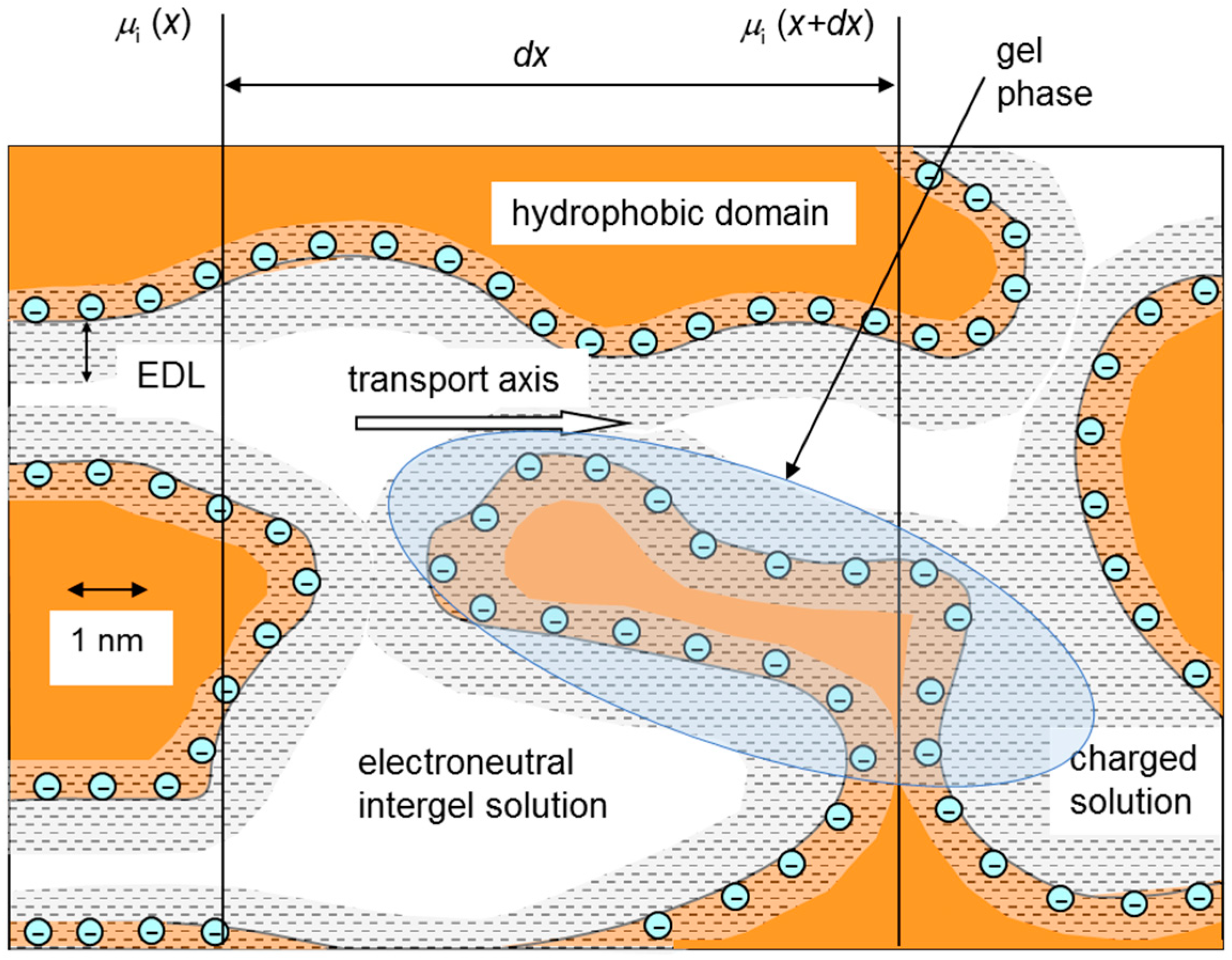
4.1.2. Multiphase Models

As it was discussed previously (Section 2), charged membranes are porous materials having generally micro-, meso- and macropores. For the definition of these types of pores, several characteristics can be applied (such as the length of action of adsorption forces) [123]. However, here we will use only one parameter to distinguish the pore type: the ratio of the pore radius, r, to the Debye length, λ, characterizing the EDL thickness at the inner pore wall. In the case of r < λ, we have a micropore (r < 1 nm); if r > λ but r and λ being of the same order of magnitude, we deal with a mesopore and if r >> λ (r > 50 nm), it is a macropore. Despite the complicated structure of charged membranes, it is important that mesopores and macropores contain electrically neutral solution in their central part, which can be considered as a separate phase (Figure 3). The properties of this solution (dielectric permittivity, ion and water diffusion coefficients) are very close to the corresponding properties of the external free solution [5,29,44]. Note that heterogeneous IEMs contain macropores, while homogeneous IEMs do not [37]. Therefore, one can expect that the volume fraction of electroneutral solution in the homogeneous membranes is essentially lower than in the heterogeneous membranes. As soon as the first electroneutral phase is defined, the remaining volume can be attributed to the second phase.

This phase, called “gel phase” [63,124], includes the polymer matrix with fixed charged groups together with mobile ions and water within the EDLs, which compensate the charge of the fixed ions. Since the central parts of the relatively large pores are excluded from the gel phase, it can be considered as a microporous relatively homogeneous medium. Sometimes, within the gel phase, one distinguishes the third phase, being the aggregate of interlaced hydrophobic polymer chains, which is not permeable for ions and solvent [63]. This hydrophobic phase may also involve the (non-conducting) inert reinforcing binder, such as polyethylene in heterogeneous membranes.

There is no distinct boundary between the inter-gel electroneutral solution and the EDL, which belongs to the gel phase. Nevertheless, the separation of the membrane material into different phases is a useful method, which allows one to simplify the mathematical description. Mafé et al. [125] carried out such a separation when applying a continuous space charge model for calculation of the membrane conductivity.

The main idea for modelling the transport within a membrane considered as a multiphase medium is in attributing some physico-chemical properties to each phase and then to describe the properties characterizing the whole membrane as functions of the single phase properties. This idea is the central one in the approach called effective medium theory (or model) [91]. Let us consider a macroscopic volume in the form of a layer of thickness dx. This layer should be sufficiently large to be “representative” and contain all phases of the membrane (Figure 3). Simultaneously, it should be small enough to allow differentiation. We neglect the detailed variations of concentrations and potential within dx and operate with the averaged quantities in the phase elements; the phases are assumed in equilibrium with one another within the dx layer.

When ion and water transfer is described in accordance with irreversible thermodynamics, by Equations (1) or (17), the problem is to obtain the effective transport coefficient L_i, which characterizes a membrane layer of thickness dx as a function of coefficients $L_i^j$ (characterizing an individual phase j), as well as the structural and geometric parameters, describing the shape and mutual position of the phases. This formulation addresses the effective-medium approach [91,126] intensively developed in relation to a great variety of systems and transfer phenomena: electrical conduction [127], diffusion [128], heat transfer [129], optics and other [130,131]. This approach was firstly applied by Maxwell [132], who, as early as in 1873, has theoretically found the conductivity of a system containing a conductive continuum medium and dispersed spheres, the conductivity of which differed from that of the medium. Later, Rayleigh, Lichtenecker, Bruggeman, Landau and Lifshitz, Mackie and Meares [133] and other [134,135] contributed to the development of effective-medium approach. The hypothesis called “principle of generalized conductivity” [135] is often applied for generalization of experimental results. According to this hypothesis, the function relating L_i to $L_i^j$ does not depend on both the nature of applied force and the nature of the transported species.

Regarding the application of this approach to IEM, several forms of functions were proposed, linking the effective conductivity of the medium with that of individual phases. Some of them relate to the diffusion [133,134], the others, the electrical conductance [124,134,136,137]. Gnusin et al. [63,74,135] developed a comprehensive model called the “microheterogeneous model” which deals with conductance coefficients L_i and $L_i^j$ instead of particular transport coefficients. Along with the membrane electrical conductivity [54,138,139,140,141,142,143], this approach also allows one to find electrolyte diffusion permeability [54,114], permselectivity (ion transport numbers) [54,144] and some other properties [74,145,146,147]. In the case of electrolyte sorption, conductivity, diffusion permeability and transport numbers, it is possible to quantitatively describe all these four characteristics as functions of bathing solution concentration starting from a single set of structural and kinetic parameters [147].

In the framework of the microheterogeneous model, the effective membrane conductance coefficient, L_i, is expressed through $L_i^j$ in the following form [63,135]:

$$L_i={\left[f_1{\left(L_i^g\right)}^{\alpha }+f_2{\left(L_i^s\right)}^{\alpha }\right]}^{1/\alpha }$$

(29)

where $L_i^g$ refers to the gel phase and $L_i^s$ to the inter-gel electroneutral solution; f₁ and f₂ are the volume fractions of the corresponding phases: f₁ = V_g/V_m, f₂ = V_s/V_m, f₁ + f₂ = 1 (where V_g, V_s and V_m are the volumes of gel, inter-gel solution and the membrane, respectively, see Figure 3); α is the structural parameter depending on the position of the phases with respect to the axis of transport: when the phases are parallel to this axis, α = 1; when they are in serial disposition, α = −1; in other cases −1 < α < 1.

When describing the transport in the gel phase, all the assumptions made in the TMS model are accepted. The properties of the inter-gel solution are assumed the same as those of the bathing equilibrium solution; the Nernst-Planck and the LEN assumption are applied there. $L_i^s$ and $L_i^g$ are expressed as functions of the ionic diffusion coefficients, $D_i^s$ and $D_i^g$ and the concentrations, $c_i^s$ and $c_i^g$ in the corresponding phase [54,63]:

$$L_i^s=D_i^s{c}_i^s/RT,L_i^g=D_i^g{c}_i^g/RT$$

(30)

Concentrations $c_i^s$ and $c_i^g$ are linked by the Donnan relations, Equation (24), the local equilibrium being assumed between both phases.

Usually the concentration of fixed ions (IEC, $\overline{Q}$) in ion-exchange materials is rather high, close to 1 mol (L wet membrane)⁻¹ or higher. Co-ions are therefore strongly excluded, so that their concentration in the gel phase is small compared to $\overline{Q}$, at least in relatively dilute solutions. When assuming ${\overline{c}}_{-}$ << $\overline{Q}$ and ${\overline{c}}_{+}\approx \overline{Q}$, Equation (24) can be simplified. In the case of a symmetrical electrolyte ($z_{+}=-z_{-}=z$) one gets [46,148]:

$${\overline{c}}_A=\frac{K_D^z}{\overline{Q}}{c}_A^2,{\overline{c}}_1=\overline{Q}+{\overline{c}}_A$$

(31)

where subscript “1” is used for the counterion; “A,” for the co-ion; c_A refers to the co-ion concentration in the inter-gel solution (assumed to be the same as the external solution).

The ions are present in both phases; the partition coefficient, K_s, involving the co-ion concentration in the membrane, $c_A^{\ast }$, can be found using Equation (31) [63]:

$$K_s=\frac{c_A^{\ast }}{c_A}=f_1\frac{K_D}{Q^g}{c}_A+f_2$$

(32)

in which the first term on the right-hand side stands for the contribution of the gel phase and the second term, for that of the inter-gel solution. $Q^g$ and K_D are the IEC of the gel phase and the Donnan coefficient, respectively. Despite of small value of f₂ (typically less than 0.1 in homogeneous membranes and close to 0.2 in heterogeneous ones), the sorption of electrolyte by the inter-gel spaces is dominant, especially in diluted solutions, because of the co-ion exclusion from the gel involving EDL in micro- and mesopores [46,148,149] is small. For conventional IEMs, Equation (31) is verified for external concentrations up to 1−2 M. Note that an equation similar to Equation (32) was proposed by Geise et al. [150], where the second term on the right-hand side of this equation was attributed to an “uncharged material,” which can sorb electrolyte stronger than the charged gel.

Equation (32) predicts a linear increase of K_s with increasing the external concentration. At low external electrolyte concentration K_s is close to f₂, that is, it value is in the vicinity of 0.1 (or lower) for the homogeneous membranes and 0.2 for the heterogeneous ones [46,148,149].

To summarize, Equations (29)–(32) form the microheterogeneous model. There are six parameters (in the case of a single electrolyte): two static, K_D and $Q^g$ (thermodynamics coefficients); two structural, f₁ and α; and two kinetic ones, the diffusion coefficients of counterion, $D_1^g$ and co-ion, $D_A^g$, in the gel phase. The diffusion coefficients in the inter-gel solution, $D_i^s$, are assumed the same as in free solution. When these parameters are known, L_i coefficients can be calculated. Then the transport membrane characteristics κ, t_i and P, can be found by using Equations (8)–(10) giving the links between the Onsager and Kedem-Katchalsky conductance coefficients. Equations (8)–(10) can be applied not only in the case, where the membrane is equilibrated with a bathing solution but also when there is a concentration gradient across the membrane. Then Equations (8)–(10) are applied at any coordinate in the membrane for a local concentration с of the inter-gel solution. In this way, it is possible to incorporate the microheterogeneous model into a boundary-value problem for modelling ion and solvent transport in membrane systems [46,151].

To obtain the microheterogeneous model’s parameters, some experiments should be carried out and the data obtained processed. To get all the six parameters listed above, the IEC, electrolyte uptake, conductivity and diffusion permeability should be determined as functions of the electrolyte concentration. The data processing algorithm is described in References [54,152]. However, often only some among the six parameters are of interest. For instance, the volume fraction of the gel phase (or inter-gel solution) is a quite important membrane characteristic. It may be relatively easily obtained from the concentration dependence of the membrane conductivity (κ). Equations (29) and (8) allows a simple approximation at $\alpha \to 0$ [63]:

$$\kappa ={\left({\kappa }^g\right)}^{f_1}{\left({\kappa }^s\right)}^{f_2}$$

(33)

Since the conductivity of gel, κ^g, only slightly depends on electrolyte concentration (since the co-ion uptake by the gel is quite low—when the external concentration is not high, usually <1 M), the lgκ − lgκ^s correlation, according to Equation (33), should be linear with f₂ as the coefficient. Numerical calculations indicate that near the “isoconductance point” (where $\kappa ={\kappa }^g={\kappa }^s$), $\kappa$ is almost independent on α [63]. In the range 0.1$c_{iso}$ < c < 10$c_{iso}$, the lgκ − lgκ^s dependence can be approximated by a straight line with slope f₂, if $\left|\alpha \right|$ ≤ 0.2. For most IEMs, α lays in the range 0.1−0.3 [37,54], hence, Equation (33) can be confidently applied, when the concentration is sufficiently close to the isoconductance concentration $c_{iso}$. Figure 4 shows Lgκ − Lgс dependencies for different IEMs taken from different papers. Since ${\kappa }^s$ is approximately proportional to the concentration of bathing solution, c, the slope of these curves should be close to f₂. Taking into account that some approximations have been made, we will call the value of f₂ found as the slope of Lgκ − Lgс linear regression the “apparent volume fraction of the inter-gel solution, f_2app”.

It can be seen from Figure 4 that the slope of linear Lgκ − Lgс approximations for the homogeneous membranes is significantly lower than this slope for the heterogeneous ones. The membranes are identified in

Table 1. Properties of some homogeneous and heterogeneous ion-exchange membranes (IEMs) in NaCl or KCl solutions. Conductivity was measured under alternative current.

Membrane	Type, Manufacturer	IEC, meq/g	Water Content, g/gdry mbr or % When in g/gwet mbr	Conductivity of Gel Phase, κg, mS cm−1	Apparent Volume Fraction of Inter-Gel Solution, f2 app
AMX, anion-exchange	Homogeneous, Neosepta Astom (Japan)	1.30 ± 0.05 [144]	0.10–0.14 [144]	3.72 * (KCl) [141] 2.19 ± 0.02 (KCl) [144] 3.2 (NaCl) [154]	0.11 * (KCl) [141] 0.099 (KCl) [144] 0.06 (NaCl) [154]
CMX, cation-exchange	Idem	1.65 [153]	0.275 [153]	8.79 * (KCl) [141] 6.72 (NaCl) [153]	0.10 * (KCl) [141] 0.06 (NaCl) [153]
CMS, cation-exchange	Idem	2.2 [146]	22–30% [146]	2.7 (NaCl) [146]	0.13 (NaCl) [146]
AMV anion-exchange	Homogeneous, Selemion Asahi Glass (Japan)	1.85 ± 0.04 [144]	0.14–0.18 [144]	3.80 ± 0.01 (KCl) [144] 3.50 (NaCl) [153]	0.06 (KCl) [144] 0.07 in NaCl [153]
Nafion 125, cation-exchange, perfluorinated	Homogeneous, DuPont™	0.81 [153]	0.129 [153]	6.70 (NaCl) [153]	0.07 (NaCl) [153]
MF-4SK, cation-exchange, perfluorinated	Homogeneous, Plastpolymer (Russia)	0.86 [153]	0.156 [153]	6.40 (NaCl) [153]	0.05 (NaCl) [153]
MA-41, anion-exchange	Heterogeneous Shchekinoazot (Russia)	1.25 [155]	0.29 [155]	3.99 * (KCl) [141]	0.24 * (KCl) [141]
MK-40, cation-exchange	Idem	2.53 [153]	0.503 [153]	5.64 * (KCl) [141] 5.27 [153]	0.25 * (KCl) [141] 0.18 [153]
LNA in NaCl	Heterogeneous, Lin’an (China)	1.63 [154]	49–55% [154]	2.2 (NaCl) [154]	0.28 (NaCl) [154]

Most measurements were made when the current flowed in the normal direction. Ref. [141] reports the results of conductivity measurements in lateral direction (shown with *).

, which contains also the values of f_2app and the conductivity of the gel phase, ${\kappa }^g$. To a first approximation (justified when the contribution of co-ions in the conductivity of the gel can be neglected), the value of ${\kappa }^g$ may be considered as a constant equal to the conductivity of the membrane at the isoconductance point.

Zabolotsky et al. [41,148] have compared the values of f₂ found from conductivity measurements when applying Equation (33) and when using other methods, namely electrolyte sorption, differential scanning calorimetry (DSC) and standard contact porosimetry [37,38,156]. Relatively close values of f₂ were reported. For example, for a heterogeneous MK-40 membrane, the authors found f₂ equal to 0.17 ± 0.02 from conductivity measurements [41], 0.10 ± 0.02 [148] and 0.26 ± 0.02 [41] from sorption, 0.21 from DSC [41] and 0.23 ± 0.05 from porosimetry [41]. These results show that the microheterogeneous model adequately describes the membrane properties when operating with reasonable structure and kinetic parameters. The ease of applying Equation (33) for processing experimental conductivity data, the possibility to determine the parameters having a clear sense, the ability to describe a set of transport properties, involving the diffusion permeability and ion transport numbers, makes this model suitable for IEMs characterization [8,37,138,142,143,144,157,158,159,160,161].

4.2. Modelling of Properties of Ion-Exchange (IEMs) Containing Nanoparticles

Recently, IEMs containing immobilized nanoparticles have attracted a keen interest in the literature. This type of membrane modification was found promising for improving IEMs used in fuel cells. It was established that Nafion based composite membranes with incorporated SiO₂, ZrO₂, TiO₂ and other nanoparticles showed better water retention and proton conductivity, especially at low water vapor pressure, in a rather large temperature interval up to 140 °C [162,163,164,165,166,167], which sometimes was accompanied with increasing IEC [168].

Yaroslavtsev et al. [169,170,171] reported that along with increasing water content and conductivity, the hybrid nanoparticle-containing membranes showed a decrease in diffusion permeability and an increase in permselectivity.

It has been shown that IEMs modification with different nanoparticles is very important not only for a better performance of fuel cells but also for improving separation processes in different industries [172]. Namely, the modification of RO, NF and ultrafiltration membranes by immobilization of inorganic nanoparticles increases their antifouling resistance [172].

Yaroslavtsev [169] suggested an interpretation of the change of membrane transport characteristics, in particular, the increase in κ by proposing a physicochemical model named the model of semielasticity of membrane pore walls. The main impact of nanoparticles on the membrane properties, according to this model, is due to the expansion of the pores and channels caused by the nanoparticles. The increase in the size of membrane channels leads to growing ion conductivity. Nevertheless, when the volume fraction of nanoparticles is too large, they block the ion conducting channels, which results in a decrease of the conductivity.

Quantitative description of the effect of nanoparticles on the transport properties of IEMs is a rather complicated problem. Filippov et al. [115,116,117] developed a fine-pore model of ion transfer in an IEM with immobilized nanoparticles. The membrane is considered as quasi-homogeneous medium as in the TMS theory and applies the approach known as the “fine porous membrane” model suggested by Starov, Churaev and Martynov [173]. The simulation was compared with experimental data on diffusion permeability of a hybrid MF-4SK membrane containing silica nanoparticles. This comparison allowed to the authors [115,116,117] to find in what extent the ion effective diffusion coefficients change in the membrane due to incorporation of silica. By applying the “fine porous membrane” model, the main membrane physicochemical parameters can be determined. In addition to the diffusion coefficients, it is possible to find the equilibrium distribution coefficients of electrolyte [117].

Porozhnyy et al. [174] proposed a mathematical model describing the effect of nanoparticles on the transport properties of membranes on the basis of the microheterogeneous model [54,63]. In addition to two phases (the gel phase and the electroneutral inter-gel solution) present in commercial membranes, there are nanoparticles. The core of a nanoparticle is non-permeable to ions and water. However, the EDL, which forms around the particle in the case where its surface is charged (Figure 5), contributes to the selective permeability of the membrane.

It is assumed that the nanoparticles are localized in the meso- and macropores; they replace there the bulk-like electroneutral solution. If the surface of nanoparticle is charged (e.g., in the case of SiO₂ or ZrO₂, where it has a negative charge), the EDL around the particle is considered to be complementary to the EDL occurring at the charged pore walls (Figure 5).

To take into account the presence of nanoparticles in a pore, the inter-gel domain is considered as a “two-phase” system containing a solution with the volume fraction $f_{sin}=\frac{V^{sol}}{V^{intergel}}$ and a solid nonconductive inclusion (the core of the nanoparticle) with the volume fraction $f_{pin}=\frac{V^{particle}}{V^{intergel}}$, where $f_{sin}+f_{pin}=1$. The effective conductance of the inter-gel domain containing a solution and a nanoparticle, $L_i^{s+p}$, may be presented, in accordance to the approach expressed by Equation (29), as

$$L_i^{s+p}={\left[f_{pin}{(L_i^p)}^{\beta }+f_{sin}{(L_i^{s1})}^{\beta }\right]}^{1/\beta }={\left(1-f_{pin}\right)}^{1/\beta }(L_i^{s1})$$

(34)

where the particle core conductance $L_i^p=0$ (the non-conductive medium), β is a structural parameter, whose role is similar to that of α in Equation (29).

$L_i^{s1}$ characterizes the solution within a pore, which can be considered again as a two-phase domain, containing the bulk electroneutral solution and the EDL, formed by the nanoparticle. $L_i^{s1}$ is found by using the same two-phase approach:

$$L_i^{s1}={\left[f_{EDLp}{(L_i^{EDL})}^{\beta }+\left(1-f_{EDLp}\right){(L_i^s)}^{\beta }\right]}^{\raisebox{1ex}{$1$}\!\left/ \!\raisebox{-1ex}{$\beta $}\right.}$$

(35)

where $f_{EDLp}=\frac{V^{EDLp}}{V^{sol+EDLp}}$ is the volume fraction of the nanoparticle’s EDL within this domain, $\left(1-f_{EDLp}\right)$ is the volume fraction of the electroneutral solution whose conductivity is, as before, assumed equal to that of the free solution.

To find $V^{EDLp}$, it is assumed that each nanoparticle is a sphere with diameter d; the size of all particles is the same. The growth of their volume fraction is achieved by increasing the number of pores where they are present.

The thickness of the diffuse part of the EDL is presented as follows:

$$L_D=\sqrt{\epsilon {\epsilon }_{0}RT/2c_i^s{z}_i^2{F}^2}$$

(36)

where $\epsilon$ is the relative dielectric permittivity, ${\epsilon }_0$ is the vacuum permittivity, $z_i$ is the ion charge number, $F$ is the Faraday constant. It is assumed that the diffusion coefficients in the nanoparticle’s EDL are the same as in the free solution, while the concentrations of cation and anion are found using the Donnan relation, as in the gel phase.

When applying Equations (34)–(36), it is possible to calculate the conductance coefficients L_i and then the membrane conductivity, electrolyte diffusion permeability, transport numbers.

The EDL formed around a nanoparticle plays an important role. It contributes to an increase in the membrane counterion conductivity, since the counterion concentration there is essentially higher than in the bulk pore solution. Increasing counterion conductivity and reduction of the concentration of co-ions (which are excluded from the EDL) results in higher membrane permselectivity. As the EDL thickness increases with decreasing the salt concentration in the external solution, its role increases; hence, the difference in membrane conductivity and permselectivity between commercial membranes and the membranes doped with nanoparticles increases with decreasing the concentration of the external solution.

However, the solid core of the nanoparticle is an insulator and this contributes to loss of the membrane conductivity at relatively high concentrations (>1 M), where the EDL thickness and, consequently, its role decrease. Thus, according to the model [174], the conductivity of nanoparticles containing membranes should be higher than that of the pristine membranes in dilute solutions. On the contrary, their conductivity should be lower than that of the pristine membranes in concentrated solutions. However, the factor of increasing pore size and water content (determined experimentally and not taken into account in the model [174]) could contribute in additional increase in conductivity. Though, as far as we know, there are no publications reporting experimental data suitable for comparison of the membrane conductivity at different concentration, in the cases where the nanoparticles are present or absent. Known publications [166,170,175] provides the conductivity of the membrane equilibrated in pure water. As for the membrane permselectivity (quantified by the counterion transport number, t₁), this parameter should be higher in the membranes doped with nanoparticles, since even when the EDL thickness is low, the increase in t₁ would be conditioned by the fact that a nonconductive nanoparticle replaces the electroneutral solution present in the inter-gel spaces. Therefore, contribution of the non-selective ion transport in this solution will be reduced in favour of highly selective transport in the charged gel phase.

The content (volume fraction) of nanoparticles in the membrane, f_p, is an important parameter. With increasing f_p, the membrane conductivity initially increases (because the total EDL volume increases), then it passes through a maximum and declines. The latter is due to the saturation of the pore space available for nanoparticles. When f_p becomes large enough, the nanoparticles block ion conductivity in the pores, which they occupy. Then ion transport occurs only across the microporous medium (the “gel phase”), which is assumed not available for nanoparticles. An example of such a dependence is given in Figure 6a. It involves experimental data for a Nafion^® membrane containing nanoparticles of caesium acid salt of phosphotungstic heteropolyacid [170] and the results of calculation according to the model described above [174]. Note that a similar dependence was found for a perfluorinated sulfocation-exchange MF-4SK membrane (analogue of Nafion^®): the proton conductivity curve as a function of additive content has a maximum at 2.6 vol%, when it is doped with SiO₂ and 1.5 vol%, when it is doped with PAni [175]. Parizian et al. [176] studied an experimental IEM modified with ZnO nanoparticles. Similarly as Safronova et al. [170] and Novikova et al. [175], they found that the dependence of water content, membrane potential, transport number and selectivity of this membrane initially increased with increasing the content of added ZnO nanoparticles, then these characteristics reach their maximum and declined when the nanoparticles’ content was rather large.

The presence of nanoparticles within the pores reduces their permeability towards the electrolyte diffusion (Figure 6b). Both the particle’s core and the EDL around it contributes to a decrease in the diffusion permeability. However, there is another factor, the expansion of pores (not taken into account in the model [174]), which gives rise to increasing membrane diffusion permeability. Which factor is determinant, depends on the membrane material (which can be more or less rigid) and the incorporated nanoparticles. Filippov, Safronova and Yaroslavtsev [115] reports an increase in the diffusion permeability of a perfluorinated sulfocation-exchange MF-4SK membrane after its doping with silica nanoparticles. Similar data are provided in Refs. [168,175].

An increase in conductivity and a decrease in diffusion permeability essentially improve the permselectivity of modified membranes towards counterions [170,174].

4.3. “Pore-flow” Models

The “pore-flow” models consider the transport of species as occurring within the membrane pores forming ion and water conducting channels [85,86]. This approach originates from the description of ion and water transport inside microcapillaries with charged walls [90,177,178,179,180]. Namely, the main goal of these models is the description of electrokinetic phenomena, that is, coupled transfer of a liquid relative to a charged solid (or liquid) surface or the transfer а charged solid particles relative to a liquid [181,182]. The main role in these phenomena is played by the EDL on charged surfaces.

The term “space-charge models” [183,184,185,186,187,188,189,190] is often applied in the literature for this kind of models. In these models, the ion and water transport is described on the basis of the Nernst-Planck-Poisson-Navier-Stokes equations. The main parameters characterizing the membrane are pore size and wall charge density [191].

The basic version of a space-charge model deals with a pore (schematically shown in Figure 7). It involves the extended Nernst-Planck equation containing the convective term, Equation (22) written in 2D geometry. The diffusion coefficients are usually assumed to be the same as in free solution. The cross-sectional distribution of local concentration, ${\tilde{c}}_i$, is described by the Poisson-Boltzman equation. The fluid flow (assumed to occur only in the axial direction) is described by the Navier-Stokes equation, where the axial pressure gradient and the electrical body force provided by the tangential electric field applied to the space charge in EDL are taking into account [177,183]. The most studies dealt with the pores whose walls are uniformly charged, such as shown in Figure 7, bottom. The impact of a non-uniform distribution of the pore wall charge on NF performance has been investigated by the group of Szymczyk in Refs. [186,192,193].

The research field making accent on the fluid transfer in narrow channels was only recently termed as nanofluidics but it has a quite rich history, in particular, in membrane science [194]. Nano- and microfluidics research as well as the applications in this field have experienced extensive growth in recent years [195,196,197,198,199]. 100 nm enables the occurrence of the phenomena, which are impossible at bigger length scales.

The “pore-flow” models involve the effects, which are specific for interfaces: change of the dielectric constant as a function of the distance from the pore wall [183], finite ion sizes, ion hydration effects [200], adsorption [185] and other [196]. These effects are taken into account when computing the streaming potential [201], diffusion permeability [186] and permselectivity [202], pore conductivity [180,203]. This type of models has been shown as very useful for describing the ion and fluid transport in and around nanometre-sized objects [204]. Bazant et al. [182,205] paid attention to the steric effects near a non-permeable wall at high voltages taking into account that solvated counter-ions are crowded there.

Cwirko and Carbonell [206] and later on Szymczyk et al. [207] have calculated using space-charge models the macroscopic Onsager’s L_ij coefficients for a Nafion membrane as functions of the membrane nanostructure parameters (which are the pore radius, pore wall charge density and the tortuosity factor). Their comparison with the experimental coefficients determined by Narebska et al. [65] has shown a rather good agreement. Thus, it becomes possible to bridge the gap between two different approaches, that is, the microscopic model description and the irreversible thermodynamics.

5. Concentration Polarization in Electrodialysis (ED)

5.1. Current-Induced Concentration Gradients

The permselectivity of IEMs towards the ions bearing the charge of a certain sign (counterions) is the main functional property [208]. Namely this property conditions the applications of this kind of membranes in ED, where the feed electrolyte solution is simultaneously demineralized and concentrated in different ED compartments (Figure 8).

When a direct current of density i flows across a membrane, concentration polarization occurs: concentration gradients arise in the boundary solution layers adjacent to the membrane. Immediately after the current is turned on, there are no diffusion fluxes, while the counterion migration flux through the membrane is higher than their flux from the solution bulk to the membrane surface. As a result, the concentration of the counterions (as well as that of co-ions) decreases at one membrane side and increases at the other. The changes of concentration near the membrane continue until the diffusion flux, which grows with time, completely compensates for the difference in migration fluxes in solution and membrane.

At any time, the flux density of species i coming from the solution and entering the membrane/solution interface is equal to the flux density leaving the interface into the membrane bulk. This condition of flux continuity is written as:

$${\left(J_i\right)}_s={\left(-D\frac{\partial c_i}{\partial x}+\frac{i{t}_i}{z_{i}F}\right)}_s=\frac{i{T}_i}{z_{i}F}$$

(37)

where ${\left(J_i\right)}_s$ is the flux density of ion i through the interface; the middle part of the Equation (37) refers to the solution: D is the electrolyte diffusion coefficient in solution, C_i and t_i are the concentration and transport number of ion i in solution; the right-hand part refers to the membrane: T_i is called integral [31,209] or effective [54,210] transport number of this ion in the membrane. T_i is defined as the current fraction carried by ion i through the interface or the membrane in steady state where no restrictions on the driving forces are imposed:

$$T_i=\frac{z_{i}F{\left(J_i\right)}_s}{i}$$

(38)

T_i can differ from the (electromigration) transport number in the membrane, $t_i^{mb}$ ($t_i$ in Equation (5) written for a membrane), since according to Equation (5), the (electromigration) transport number must be determined under the condition that the concentration gradient and the convective flow across the membrane are zero. Nevertheless, if the external solution concentration is not too high, T_i is quite close to $t_i^{mb}$. Normally, commercial membranes are highly permselective to counterions [76]: the values of T₁ and $t_i^{mb}$ approach 1 when the solution is diluted.

According to classical electrochemistry, the occurrence of concentration gradients near the surface of a membrane (or an electrode) results from the limitation of the current density i. With increasing i, the electrolyte concentration at the interface, c_s, decreases (Figure 8). When c_s approaches zero (becomes much smaller than the bulk concentration, c⁰), the current density reaches its limiting value (i_lim). The expression for i_lim can be obtained from Equations (37), (38), when writing the concentration gradient of the counterion (1) at the membrane surface as:

$${\left(\frac{\partial c_1}{\partial x}\right)}_s=-\frac{c_1^0-c_{1s}}{\delta }$$

(39)

where $\delta$ is the thickness of the Nernst DBL in the depleted solution. According to Equation (39), $\delta$ is the distance from the membrane to the intersection point of the tangent drawn to the concentration profile at the interface with the line corresponding to the bulk solution concentration. Substituting Equation (39) into Equation (37) and setting c_1s = 0 yields:

$$i_{\lim }=\frac{FD{c}^0}{\delta (T_1-t_1)}$$

(40)

where c⁰ = $z_{+}{c}_{+}^0=-z_{-}{c}_{-}^0$ is the bulk electrolyte concentration in eq L⁻¹. Equation (40) was first obtained by Peers in 1956 [211].

According to the classical theory [57] based on the LEN assumption, when i tends to its limiting value (i_lim), the PD over a membrane surrounded by two DBLs tends to infinity. However, in real membrane or electrode systems, the limiting current density can be exceeded in several times [212,213,214,215]. The causes of the overlimiting current are vividly discussed in literature [212,214,216,217,218,219]. The main effects are current-induced convection (electro- and gravitational convection) and generation of additional charge carriers (e.g., water splitting at the depleted solution/membrane interface, which produces the H⁺ and OH⁻ ions). While current-induced convection enhances the mass transfer across the membrane, water splitting in most cases is undesirable effect causing pH changes and the loss in current efficiency.

Experimental observations [212,220,221,222,223,224,225,226,227,228,229] as well as theoretical evidences [216,230,231] show the dominant role of electroconvection in salt counterion overlimiting transfer in dilute solutions. Vortices, which appear under the action of electric field on the space charge, can increase the useful transfer of salt counterions in several times by mixing depleted solution [217,230,232,233].

Along with these two main effects, additional effects, which may occur in some conditions, are discussed in literature. Andersen et al. [234] described theoretically the effect of current-induced membrane discharge. This effect can occur in a system with an AEM, which has weakly basic functional groups. In this case, OH⁻ ions generated in water splitting at the depleted membrane interface may deprotonate these functional groups, that is, discharge them. This produces: (1) a decrease in the surface charge density, which reduces electroconvection developing as electroosmosis of both the 1st and 2nd kind [235,236] and (2) a decrease in IEC, which results in increasing co-ion back diffusion through the membrane. The latter leads to a decrease in T₁, hence, in an increase of the limiting current density according to Equation (40). Note that electroosmosis of the 2nd kind is named also induced-charge electroosmosis [237,238], since this effect is due to the extended space charge region [239], which emerges next to the equilibrium EDL at overlimiting currents.

In the early period of ED, the use of underlimiting current was prescribed [210,240]. However, nowadays the overlimiting current regimes are widely used in ED and especially in electro-deionisation of diluted electrolyte solutions [212,241]. The use of such intensive current regimes allows reduction of expensive membranes’ area, which can cause the reduction of overall costs of ED desalination [210]. The effect of electroconvection is relevant also in a number of nano- and microfluidic devices [194,242] such as electrokinetic micropumps [243,244]. Besides, intensive current regimes are applied in electrophoresis [242], electrodeposition [245], layering of colloid crystals on electrode surfaces [246] and other domains related to separation science [58,203].

5.2. 2D Modelling of Electrodialysis with Homogeneous Membranes

5.2.1. Governing Equations and General Boundary Conditions

The first adequate 2D model of ED (named the hydrodynamic theory of desalination) was developed by Sonin and Probstein [247]. Later on other versions of this model was proposed, in particular, by Gnusin et al. [248,249] and Tedesco et al. [250], who reported a numerical solution of the problem formulated by Sonin and Probstein, when taking into account the difference in the diffusion coefficients of cation and anion in solution; Shaposhnik et al. developed an analytical solution for special cases [251] and accounted for the effect of ion-conducting spacer in numerical solution [252].

Solan et al. [253,254] proposed a “mesh step” model for the effect of a net type spacer—turbulence promoter—on mass transfer in an ED channel. The role of spacer in ED desalination was also studied by a number of authors [255,256,257,258,259,260,261]. Other aspects of modelling of ED are considered in Refs. [262,263] and other contributions are reviewed by Campione et al. [264].

The basic version of 2D mathematical model of ED involves [247,248,249] the extended Nernst-Planck equation (Equation (22)) in vector form, the equation expressing the current density as a sum of ion flux densities (Equation (23)), the continuity equation for the conservation of species i written for the steady state) and the LEN condition:

$${\overrightarrow{j}}_i=-D_i\left(\nabla c_i+z_i{c}_i\frac{F}{RT}\nabla \phi \right)+c_i\overrightarrow{V} ,i=1,2$$

(41)

$$i=F{\displaystyle \sum z_i{j}_i}$$

(42)

$$div{\overrightarrow{j}}_i=-\frac{\partial c_i}{\partial t}=0,$$

(43)

$${\displaystyle \sum z_i{c}_i}=0$$

(44)

The system of coordinates is shown in Figure 8.

Equations (41)–(44) are written for a cation and an anion denoted by subscript i as 1 and 2, respectively.

It is assumed that the fluid velocity at the surface is zero (the no-slip condition) [80]:

$$\overrightarrow{V}(x=0,y)=0,\overrightarrow{V}(x=h,y)=0$$

(45)

The fluid flow is considered laminar and steady.

For such a flow between two parallel plates (without spacer), the solution of the Navier-Stokes equation with the boundary no-slip condition gives a parabolic velocity distribution along the transverse coordinate known as the Poiseuille distribution, the normal component of flow velocity is zero:

$$V_x=0,V_y(x)=6\overline{V}\left(\frac{x}{h}-\frac{x^2}{h^2}\right)$$

(46)

where $\overline{V}$ is the average flow velocity between the plates.

The continuity of the ion fluxes through the interface (Equation (37)), which is rewritten in the form

$${\left(\frac{\partial c}{\partial x}\right)}_{x=0}=\frac{i(T_1^c-t_1)}{FD},{\left(\frac{\partial c}{\partial x}\right)}_{x=h}=-\frac{i(T_2^a-t_2)}{FD}$$

(47)

is used as the boundary condition for both AEM and CEM. Note that the effective transport numbers of cations in the CEM ($T_1^c$) and anions in the AEM ($T_2^a$) can take into account the co-ion or H⁺(OH⁻) transport across the membrane. For this, experimental [76,265] or theoretical [266] evaluation of $T_1^c$ and $T_2^a$ should be carried out.

The feed solution concentration at the channel entrance is set as the initial condition:

$$c(x,0)=c_0$$

(48)

The condition specifying the parameters of the operating mode assumes that the PD Δϕ between two planes passing through the centre of two nearest concentration compartments (CC) is known. This PD can be found as Δϕ =(U − Δϕ_el)/n, where U is the voltage measured between the polarizing electrodes of the ED cell, Δϕ_el is the PD on the electrodes and n is the number of cell pairs. It is assumed that any plane passing through the centre of an CC is equipotential and the current density and ionic fluxes along this plane are zero.

The PD per a cell pair (considered as a known parameter) is determined by the equation:

$$\Delta \phi =-i(R_a+R_c+R_{cc})+\Delta {\phi }_D+{\displaystyle \underset{0}{\overset{h}{\int }}E}dx$$

(49)

where R_a, R_c and R_cc are the resistances of the AEM, CEM and the concentration compartment, respectively (all are assumed known), $\Delta {\phi }_D$ is the sum of (Donnan) PDs over the solution/membrane interfaces for AEM and CEM, $E=-\frac{\partial \phi }{\partial x}$ is the electric field; ${\displaystyle \underset{0}{\overset{h}{\int }}E}dx$ is the PD in the DC. The diffusion transport in the membranes and the CC is not taken into account, the $\overrightarrow{i}$ and $\overrightarrow{E}$ vectors are assumed directed normally to the membrane surface. According to Equation (27),

$$\Delta {\phi }_D(y)=-\frac{RT}{z_{1}F}\ln \frac{c(0,y)}{c_0}--\frac{RT}{z_{2}F}\ln \frac{c_0}{c(h,y)}$$

(50)

Equations (41)–(49) form a 2D boundary value problem under the condition that E(x,y) is expressed as a function of electrolyte concentration c(x,y) and current density i(x,y).

Taking into account the condition $V_x=0$, the x-component of Equation (41) is written as the conventional Nernst-Planck equation. The electric field strength can be found from Equations (41), (42) and (43):

$$E=\frac{RT}{F}\left[\frac{D_1-D_2}{D_1{z}_1-D_2{z}_2}\frac{\partial c}{c\partial x}+\frac{i}{\left(D_1{z}_1-D_2{z}_2\right)cF}\right]$$

(51)

where $c=z_1,c_1=-z_2{c}_2$ is the electrolyte concentration (in eq L⁻¹).

Substituting Equation (51) into Equation (41) yields the transport equation in the (reduced) form of Kedem-Katchalsky equation (Equation (5)):

$$j_i=-D\frac{\partial c_i}{\partial x}+\frac{i{t}_i}{z_{i}F}$$

(52)

where D (the electrolyte diffusion coefficient) and $t_k$ (the transport number of ion k) are expressed as follows:

$$D=(z_1-z_2)D_1{D}_2/(D_1{z}_1-D_2{z}_2)$$

(53)

$$t_i=z_i{D}_i/\left(z_1{D}_1-z_2{D}_2\right)$$

(54)

In the vector form when taking into account the convective term, Equation (52) reads as follows:

$${\overrightarrow{j}}_i=-D\nabla c_i+\frac{\overrightarrow{i}{t}_i}{z_{i}F}+c_i\overrightarrow{V}$$

(55)

When considering the normal and longitudinal components of ${\overrightarrow{j}}_i$, it is assumed that the normal velocity is zero and the longitudinal diffusion and migration are negligible compared to the convective transport:

$$j_{ix}=-D\frac{\partial c_i}{\partial x}+\frac{i{t}_i}{z_{i}F}$$

(56)

$$j_{iy}=c_{i}V(x)$$

(57)

Then the application of Equation (43) to Equation (55) gives [80]:

$$D\frac{{\partial }^{2}c}{\partial x^2}=V(x)\frac{\partial c}{\partial y}.$$

(58)

Here for the sake of simplicity, V(x) refers to the longitudinal velocity. The diffusion coefficient and the transport numbers are assumed constant and known quantities.

5.2.2. Concentration Distribution and Diffusion Layer Thickness

Numerical solution of the convection-diffusion problem presented by Equations (45)–(49) and (58) gives the distribution of concentration c(x,y), current density i(y) and electric potential ϕ(x,y) in the space between an AEM and CEM under the condition that the overall PD per cell pair Δϕ is known and the geometric parameters of the cell as well as the average flow velocity are set. In the version presented above, the variation of concentration for the sake of simplicity is taken into account only in the DC since namely this compartment determines the behaviour of the system in ED desalination: the concentration variations in the CC only slightly affect the overall system resistance.

The concentration profiles in the DC computed at different distances from the cell entrance are shown in Figure 9.

It can be seen that the concentration profiles are not symmetric, which is due to the difference in the transport numbers of cation and anion leading to a difference in the concentration gradients at the AEM and CEM, according to Equation (47) used as the boundary condition for the problem. Despite the difference in the concentration gradients, the thickness of the Nernst DBLs (determined through the intersection point of tangents to the concentration profiles, Equation (39)) at a AEM and CEM are the same, and, in the first approximation, do not depend on the applied voltage [248].

When a sufficiently great PD is applied, the concentration at the surface of the membrane, for which the difference of counterion transport numbers $(T_i-t_i)$ is maximum, reaches a nearly zero value, the average current density for this membrane (the CEM in the case of NaCl) attains the limiting value, Equation (40). Subsequent growth of Δϕ does not lead to an increase in the current density. When the current density is limiting, the problem (45)–(49) and (58) can be simplified. Instead of the boundary condition of the second kind [Equation (47), expressing the concentration gradient at the membrane surface], the boundary condition of the first kind, the concentration equal to zero at this surface, can be used:

$$c{(0,y)}_{y>0}=0$$

(59)

This simplified boundary value problem can be solved approximately. Indeed, an asymptotic solution was obtained by Lévêque in the case of the diffusion-convection heat transfer [267]. Adapting this solution to diffusion-convection mass transfer gives [80]:

$$i_{\lim loc}(y)=\frac{FD{c}_0}{h(T_1-t_1)}\left[0.978{\left(\frac{h^2{V}_0}{yD}\right)}^{1/3}-0.2\right],i_{\lim av}(L)=\frac{FD{c}_0}{h(T_1-t_1)}\left[1.47{\left(\frac{h^2{V}_0}{LD}\right)}^{1/3}-0.2\right]$$

(60)

where $i_{\lim loc}$ and $i_{\lim av}$ are the local and the average over the channel length (L) current densities, respectively; $i_{\lim av}=\frac{1}{L}{\displaystyle \underset{0}{\overset{L}{\int }}{i}_{\lim loc}\left(y\right)dy}$, where y is the distance from the channel entrance.

Combining Equations (60) with the Peers equation, Equation (40), yields the following equations for the local, ${\delta }_{Nloc}$ and the average, ${\delta }_{Nav}$, values of the Nernst DBL thickness, ${\delta }_N$, in the case where the second term (“0.2”) in brackets on the right-hand side is neglected [248,268]:

$${\delta }_{Nloc}=1.02h{\left(\frac{LD}{h^2{V}_0}\right)}^{\raisebox{1ex}{$1$}\!\left/ \!\raisebox{-1ex}{$3$}\right.},{\delta }_{Nav}=0.68h{\left(\frac{LD}{h^2{V}_0}\right)}^{\raisebox{1ex}{$1$}\!\left/ \!\raisebox{-1ex}{$3$}\right.}$$

(61)

As it can be seen from Equations (60), the relative contribution of the “0.2” term on the right-hand side decreases with decreasing the channel length L. However, similar equations can be obtained by treating the values of i_lim or ${\delta }_N$ found numerically from a convection-diffusion problem where zero concentration at the wall is used as the boundary condition. In this case, the limiting current density is in excellent agreement with Equations (60), while the values of the local and average ${\delta }_N$ are slightly (about 4%) higher than those presented by Equations (61) due to the effect of the omitted second term. Namely, instead of 0.68 and 1.02, the numerical solution gives 0.71 and 1.06, for the local and the average ${\delta }_N$, respectively [269].

Equations (60)–(61) are verified only for “short” channels where $L\le 0.02h^2{V}_0/D$ (or $Y=LD/\left(\overline{V}{h}^2\right)\le 0.02$) [248].

Taking into account the definition of $i_{\lim av}$ above and the fact that i_lim and ${\delta }_N$ are inversely proportional to each other, Equation (40), we can arrive at the meaning of the average value of Nernst’s DBL thickness: ${\delta }_{Nav}^{-1}=\frac{1}{L}{\displaystyle \underset{0}{\overset{L}{\int }}{\delta }_{Nloc}^{-1}\left(y\right)dy}$. On the other hand, ${\delta }_{Nav}$ can be also understood as the effective DBL thickness, ${\delta }_{Nef}$, in a channel where ${\delta }_N$ is a function of the distance from the entrance: the substitution of ${\delta }_{Nav}$ in the Peers equation, Equation (40), gives the correct value of $i_{\lim av}$.

The mass transfer rate in an ED channel at the limiting current can be also expressed in terms of the Sherwood, Reynolds and Schmidt numbers [80,248]:

$$Sh=1.23{[ReSc(2h/L)]}^{1/3}-0.4,S{h}_{av}=1.85{[ReSc(2h/L)]}^{1/3}-0.4$$

(62)

where

$$Sh=\frac{i_{\lim }2h(T_1-t_1)}{FD{c}_0}=\frac{2h}{{\delta }_N},Re=\frac{2h\overline{V}}{\nu },Sc=\frac{\nu }{D}$$

(63)

Sh_av is the average value of Sh in a channel of length L, ν is the kinematic viscosity.

For an ED channel of a dimensionless length $Y=\frac{LD}{h^2{V}_0}$ = 0.01, the local and average DBL thicknesses reach 0.23h and 0.15h, respectively; the degree of desalination at the limiting current density is 10–13% (it depends on the type of electrolyte). These values are typical for “short” channels in cells commonly used for electrochemical studies of IEMs. For “long” channels, where the DBLs formed at the AEM and CEM are overlapped, it is possible to use numerically calculated Sh vs. Y curves [248]. For rough estimations of the local limiting current density using Equation (40), the effective average value of ${\delta }_N$ can be taken equal to h/3.

Equations (60) agree well with the experimentally determined limiting current density in a cell specially designed [270] to satisfy the conditions required for obtaining this equation. The cell has the input and output comb-like devices, which assure the laminar flow for the average velocities from 10⁻² cm/s to 2 cm/s. The intermembrane distance (h = 5−6 mm) and the channel length (20 mm) give the dimensionless length Y in the interval 10⁻⁵–10⁻², where the Lévêque approximations (Equations (60)) are well satisfied. The possibility of knowing the theoretical limiting current density and the DBL thickness is very important, as it allows evaluation the coupled effects of concentration polarization. Indeed, the theoretical values of i_lim and δ are determined for the case of an “ideal” IEM, which does not generate current-induced convection and does not split water molecules. Hence, the comparison of the experimental and theoretical i_lim can give some ideas, for example about the intensity of electroconvection [217]. The role of the Lévêque equations for the slot cells with laminar flow is similar to the Levich equation obtained for the rotating disk electrode [271] or rotating membrane disc [225,272,273].

5.3. ED with Heterogeneous Membranes

Competition between homogeneous and heterogeneous IEMs lasts for decades. Although the conductivity and permselectivity of a heterogeneous IEM is generally lower than these parameters of a homogeneous membrane, the great advantage of heterogeneous IEMs is that they are less costly.

The surface of heterogeneous membranes includes conductive and non-conductive areas of the size from several μm to several tens of μm. The so called homogeneous membranes (usually prepared the paste method via copolymerization [9]) also contain non-conductive inclusions (e.g., PVC binder), however, the size of these inclusions generally less than 1 μm (except the threads of backing cloth). For instance, the Neosepta^® AMX and CMX membranes have PVC particles with a diameter of about 100 nm. The presence of non-conductive areas leads to the accumulation of the electric current lines on the conductive regions and to the curvature of these lines. On one hand, this “funnel effect” [274] increases membrane concentration polarization and water splitting rate, while reducing the limiting current density [274]. On the other hand, tangential electric field enhances electroconvection and mass transfer [232,236,275,276]. From what has been said before, the electrical heterogeneity of the membrane surface is subject to optimization. Too low surface fraction of membrane conductive area (γ) will lead to very high concentration polarization, which could be remediated by electroconvection. However, one can imagine that a certain heterogeneity of the surface could effectively enhance electroconvection, while only slightly increase concentration polarization. Simulations made by Davidson et al. [233] and Zabolotsky et al. [272] predict that the rate of electroconvection and, as a consequence, the rate of mass transfer pass through a maximum with increasing γ at a fixed voltage. According to [233], the maximum is close to γ = 0.5; according to [272], it is close to γ = 0.8. The both models are based on the same governing equations (the Nernst-Planck-Poisson-Navier-Stokes equations). Perhaps, the difference is due to the fact that Davidson et al. [233] do not take into account the forced flow between the membranes, while Zabolotsky et al. [272] do.

Another important lever for enhancing electroconvection and mass transfer is geometric heterogeneity (surface undulation, waviness, formation of special patterns). However, this option is still poorly studied, which can be understood in view of the wide variety of possible geometric shapes and sizes. A deeper understanding of the peculiarities of ion and water transport at electrically and geometrically heterogeneous surface is needed for targeted optimization of membrane surface parameters. Later on we will consider some aspects of mathematical modelling of ion transport at heterogeneous membrane surface.

Effect of Electrical Surface Heterogeneity on the Limiting Current Density and Diffusion Layer Thickness

Consider an ED channel, which is formed by a homogeneous AEM (which may have areas on their surface that differ in conductivity but the size of these areas is less than 1 μm) and a heterogeneous CEM whose surface contains alternating conductive and non-conductive areas, whose size is of the order of 10 μm or more. Figure 10 gives a 2D schematic presentation of such a channel. The length of the conductive region on the surface is denoted as 2b, the distance between the centres of two nearest conductive regions (the spatial period of surface heterogeneity) is 2l. As earlier (Section 5.2), we assume that a binary electrolyte solution with initial concentration c₀ flows between the membrane, the flow being laminar and there is Poiseuille velocity distribution, Equation (46). A PD $\Delta \phi$ is applied between two planes passing through the centres of the concentration compartments adjacent to the central DC.

The governing equations used here are the same as in the case of homogeneous membranes: the Nernst-Planck with the convective term, Equation (41) and the continuity equation for the electrolyte species, Equation (43). However, instead of the LEN assumption, Equation (44), we use here the Poisson equation:

$$\epsilon {\epsilon }_0\nabla ·\overrightarrow{E}=-\epsilon {\epsilon }_0{\nabla }^2\phi =F{\displaystyle \sum _i{z}_i{c}_i}$$

(64)

where ${\epsilon }_0$ and $\epsilon$ are the vacuum permittivity and the relative permittivity of the solution, respectively.

As for the boundary conditions, as in Section 5.2, we assume the continuity of the fluxes across both conductive and non-conductive regions. Both CEM and AEM are considered as “ideally selective”: the current is carried solely by counterions, hence, at the solution/membrane interface, the counterion partial current density is equal to the total current density and the co-ion normal flux is zero. In addition, following Rubinstein and Shtilman [239], we set the counterion concentration at the conductive surface regions (c_1m at the CEM and c_2m at the AEM, their values are considered as parameters). This condition may be called the Dirichlet-Rubinstein boundary condition [214]. It is applied also by Pham et al. [277] and Kwak et al. [230]. Hence, for the conductive surface regions of the CEM and the whole surface of the AEM, we have:

$$\begin{array}{c}\left(\frac{\partial c_1}{\partial x}+\frac{F}{RT}{z}_1{c}_1\frac{\partial \phi }{\partial x}\right)\left(0,y_{cond}\right)=\frac{i_x\left(0,y_{cond}\right)}{D_{1}F},\left(\frac{\partial c_2}{\partial x}+\frac{F}{RT}{z}_2{c}_2\frac{\partial \phi }{\partial x}\right)\left(0,y_{cond}\right)=0,\\ c_1\left(0,y_{cond}\right)=c_{1m}=N_c{c}_0\end{array}$$

(65)

$$\begin{array}{c}\left(\frac{\partial c_1}{\partial x}+\frac{F}{RT}{z}_1{c}_1\frac{\partial \phi }{\partial x}\right)\left(h,y\right)=0,\left(\frac{\partial c_2}{\partial x}+\frac{F}{RT}{z}_2{c}_2\frac{\partial \phi }{\partial x}\right)\left(h,y\right)=-\frac{i_x\left(0,y\right)}{D_{2}F},\\ c_2\left(h,y\right)=c_{2m}=N_a{c}_0\end{array}$$

(66)

where N_a and N_c show how many times $c_{2m}$ and $c_{1m}$ are higher than the inlet electrolyte concentration (c₀), respectively. Subscript “cond” refers to a conductive surface region.

The boundary conditions for the non-conductive regions of the CEM set zero normal flux across the surface:

$$j_{ix}\left(0,y_{non-cond}\right)=0,i=1,2$$

(67)

When writing $\left(\frac{\partial c_i}{\partial x}+\frac{F}{RT}{z}_i{c}_i\frac{\partial \phi }{\partial x}\right)\left(0,y_{non-cond}\right)=0$ for both ions and taking into account that the LEN condition holds in the solution at the insulating surface, one finds that condition (66) leads to zero normal components of both concentration and potential gradients: $\frac{\partial \phi }{\partial x}\left(0,y_{non-cond}\right)=0$ and $\frac{\partial c_i}{\partial x}\left(0,y_{non-cond}\right)=0$.

It is assumed that the electric current does not flow through the channel entrance and the channel exit. At the channel entrance, the electrolyte concentration is given and the LEN condition holds. At the exit, the tangential diffusion is negligible: ions can leave the channel only with the convective flow. This gives the following conditions:

$$\frac{\partial \phi }{\partial y}\left(x,0\right)=0,c_i\left(x,0\right)=c_{i0}$$

(68)

$$\frac{\partial \phi }{\partial y}\left(x,L\text{}\right)=0,j_{iy}\left(x,L\right)=c_{i}V(x)$$

(69)

As in the case of homogeneous membranes (Section 5.2), the electric mode operating parameter is the PD between two planes in the centres of CC. However, when applying the Poisson equation, the electric potential is set at the surfaces of both IEMs. Similar to Equation (49), the total PD in an ED cell pair (Δϕ) is presented as the sum of three contributions:

$$\Delta \phi =\Delta {\phi }_a+\Delta {\phi }_{DC}+\Delta {\phi }_c$$

(70)

where $\Delta {\phi }_{DC}$ is the PD within the desalination compartment limited by x = 0 at the left and x = h at the right, $\Delta {\phi }_a$ is the PD across the AEM and a half of the concentration compartment, $\Delta {\phi }_c$ is a similar quantity for the CEM half-cell (Figure 11).

To find $\phi \left(0,y\right)$ and $\phi \left(h,y\right)$ as functions of the normal local current density ($i_x$) and Δϕ, it is assumed [214] that between the point referred to the membrane surface facing the CC and the point on the surface facing the DC where the counterion concentration is set (x = 0 for the CEM and x = h for the AEM, Figure 11), there is the membrane bulk and two interfacial quasi-equilibrium EDLs [83,214]. The PD between these two points is the sum of the ohmic PD and two Donnan PDs. For the sake of simplicity, concentration polarization at the membrane interfaces with enriched solution is not taken into account, hence, everywhere in the concentrating compartment the concentration is set equal to c₀. Under these assumptions, the PD between the plane passing through the centre of the CC and x = 0, $\Delta {\phi }_c$ and the PD between the plane passing through the centre of the CC and x = h, $\Delta {\phi }_a$, read as follows [214]:

$$\Delta {\phi }_c=-\frac{1}{2}{R}_{ms}{i}_x(0,y_{cond})-\frac{RT}{z_{1}F}\ln \frac{c_{1m}}{c_0}=-\frac{1}{2}{R}_{ms}{i}_x(0,y_{cond})-\frac{RT}{F}\ln N_c$$

(71)

$$\Delta {\phi }_a=-\frac{1}{2}{R}_{ms}{i}_x(h,y_{cond})-\frac{RT}{z_{2}F}\ln \frac{c_0}{c_{2m}}=-\frac{1}{2}{R}_{ms}{i}_x(h,y_{cond})-\frac{RT}{F}\ln N_a$$

(72)

where $R_{ms}$ is the total ohmic (membrane+solution) resistance of the system involving an AEM and a CEM as well as a concentration compartment. Equations (71) and (72) are written only for the conductive regions on the CEM surface. The second terms on the left-hand side of Equations (71) and (72) involve the total interfacial PD. Thus, for the CEM, we have

$$\Delta {\phi }_c^{Don}=-\frac{RT}{z_{1}F}\ln \frac{{\overline{c}}_1}{c_0}-\frac{RT}{z_{1}F}\ln \frac{c_{1m}}{{\overline{c}}_1}=-\frac{RT}{F}\ln \frac{c_{1m}}{c_0}=-\frac{RT}{F}\ln N_c$$

(73)

Setting ϕ = 0 in the middle of the left-hand concentration compartment and taking into account that $\phi (0,y)=\Delta {\phi }_c$ and $\Delta \phi =\phi (h,y)+\Delta {\phi }_a$, we find from Equations (71) and (72):

$$\phi \left(0,y_{cond}\right)=-\frac{1}{2}{R}_{ms}{i}_x\left(0,y_{cond}\right)-\frac{RT}{F}\ln N_a,\phi \left(h,y\right)=\Delta \phi +\frac{1}{2}{R}_{ms}{i}_x\left(h,y\right)+\frac{RT}{F}\ln N_a$$

(74)

The positions of the cross-sections for which the profiles are calculated are shown in Figure 12; the first cross-section is at 550 μm from the entrance; the intermembrane distance h = 1000 μm; the average flow velocity of solution in the channel between the membranes is 0.08 cm·s⁻¹; the length of the conductive surface regions is fixed: a = 10 μm.

The part of the concentration profile close to the surface changes essentially when passing from one cross-section to another along the y-axis (Figure 13). At the centre of the conductive region, the normal component of the concentration gradient (the slope of the concentration profile) is maximum, while it is zero at the centre of the non-conductive region. However, at some distance from the surface the changes of the concentration gradient slope with y are rather small: this slope gradually decreases as the distance from the entrance increases. Thus, it is possible to define the effective DBL thickness ${\delta }_N^{\prime }$ from the concentration profile slope at a distance d from the surface, where the changes in the slope caused by the surface being conductive or not are negligible:

$${\delta }_N^{\prime }=d+\left[c_0-c\left(d\right)\right]/{\left(\frac{\partial c_1}{\partial x}\right)}_{x=d}$$

(75)

For a homogeneous membrane, d = 0 and Equation (75) gives the quantity, which is identical to the Nernst DBL thickness, as c(d) is the concentration at the membrane surface. Together with the Nernst DBL, the total DBL thickness, δ_tot, is often used. δ_tot can be defined [268], as the distance from the surface to the point in solution where c = 0.99c₀. The results of the computations of ${\delta }_N^{\prime }$ and δ_tot for the cross section at a distance of 550 μm from the ED channel entrance are shown in

Table 2. Thickness of the DBL determined numerically for cross section 1 (Figure 12) passing across the centre of the conductive region at a distance of 550 μm from the ED channel entrance at different values of the fraction of conductive surface area, γ.

γ	${\mathit{\delta }}_{\mathit{N}}^{\prime },\mathsf{\mu }\mathbf{m}$	δtot, μm
0.1	54	128
0.2	72	134
0.5	86	136
1	85	139

.

6. Effect of Surface Heterogeneity on the Transient Behaviour of IEMs

6.1. Modelling of Chronopotentiograms for Homogeneous Membranes. Effect of Finite-Length Diffusion Layer

When a current of density i is applied to an IEM initially in an equilibrium state with the bathing solution, the concentration profiles develop with time [12,31,278]. Electrolyte diffusion from the solution bulk to the membrane surface arise and the diffusion flux of counterions is added to their migration in solution, which slows down the rate of concentration changes at the interface. If the current density is not high (lower than the steady-state limiting current density, i_lim), the electrolyte diffusion reaches such a rate, that the difference between the counterion migration fluxes in the membrane and solution gets compensated. The system reaches a steady state whereas the main mechanism of current transfer remains electrodiffusion. However, if the current density is higher than i_lim, at a certain time called “transition time” there is a change in current transfer mechanism across the membrane. At i > i_lim, the electrolyte diffusion is not sufficient to stop the decrease of concentration at the membrane interface. When the electrolyte concentration at this interface reaches a rather small critical value [216,277], current-induced mechanisms of overlimiting current conductance such as coupled convection (gravitational convection and electroconvection), water splitting [24,220,279] and others [213,234] occur additionally to the electrodiffusion. Current-induced convection enhances the delivery of electrolyte to the membrane surface [217,230,232]. Since the rate of electrolyte delivery via current-induced convection increases as the current density increases, the system reaches a steady-state where its resistance is higher than that at i < i_lim but remains finite.

The onset of these additional transport mechanisms occurs in the vicinity of the transition time τ, which corresponds to the inflection point on the chronopotentiogram. The rate of increase of the PD across the membrane attains its maximum. After reaching the transition state (t = τ), the rate of PD increase slows down. Then the system reaches a steady state where the PD does not change (or slowly changes) with time. The current-induced mechanisms of ion transport result in reducing concentration polarization. Even when the current density is higher than i_lim, the ion concentration at the interface never reaches zero and PD is not tends to infinity [239,280].

Chronopotentiometry (CP) is a method of studying the transient behaviour of electrode and membrane systems, when a (constant) current density is applied and the response of time-dependent PD is measured. It is a powerful technique for studying interfacial ion transport and chemical reactions [15,278,281,282].

The transition time is an important characteristic of time-dependent ion transport [15,282,283]. In 1901 Sand [284] deduced a simple equation for the transition time, τ, when considering diffusion in a semi-infinite 1D domain with a constant-flux boundary condition:

$$\tau =\left(\frac{\pi D}{4}\right){\left(\frac{c_{i0}{z}_{i}F}{T_i-t_i}\right)}^2\frac{1}{i^2}$$

(76)

The adaptation of the Sand equation to IEMs with non-ideal permselectivity expressed by T_k was first made apparently by Lerche and Wolf [285] and later by Krol et al. [282].

In Sand’s theory, the DBL thickness is assumed infinite; the forced or natural convection occurring in the membrane/electrode system is not taken into account. The transition time is defined as the moment where the interfacial concentration attains zero and the PD tends to infinity.

The fact that the DBL thickness is assumed infinite leads to essential deviation between theoretical and experimental values of in certain conditions. The situation is similar to that in the theory of impedance. Warburg [286] proposed a simple theory for computing the impedance of solution/electrode system as a function of frequency assuming that the DBL thickness is infinitely large. However, taking into account the finite length of the DBL changes cardinally the shape of impedance spectrum [287,288]. The finite length of the DBL at membrane surface was accounted by Sistat and Pourcelly [289] and Larchet et al. [46], when basing on the Nernst-Planck equation and the LEN assumption. The value of the DBL thickness, δ, is considered as a fitting parameter. In Reference [46], the time dependence of δ is implicitly taken into account in conditions of current-induced gravitational convection. Recently, van Soestbergen et al. [290] presented a theory based on the Nernst-Planck-Poisson equations. The value of δ was fixed as the distance between two parallel electrodes forming the cell; electron-transfer reactions across the Stern monolayer at the electrode surface were taken into account [290]. Mareev et al. [269] took into account the decrease of δ, occurring with time, due to the development of current-induced convection. The value of δ is considered as a function of the Donnan PD (Δϕ_Don) at the membrane/depleted solution interface. When an overlimiting current density is applied and the time approaches the transition time, current-induced convection (namely, electroconvection) arises near the depleted interface and causes a decrease of δ. The δ(Δϕ_Don) function is assumed a linear one containing two adjustable parameters: a threshold value of Δϕ_Don, which relates to the onset of electroconvection and a value of Δϕ_Don related to the steady state.

As it is shown in Reference [269], the model describes well experimental chronopotentiograms of a CMX homogeneous CEM at all applied overlimiting current densities. The comparison of the calculation using the Sand theory and the model [269] with experimental transition times found for different current densities is shown in Figure 14. As it can be seen, the Sand transition time is less than the experimental value; this difference increases with decreasing (overlimiting) current density. The explanation is that the assumption of the semi-infinite DBL does not allow accounting for the contribution of forced (or natural) convection. The electrolyte delivery by convection slows down the growth of PD with time. However, when the current density is sufficiently high (>1.5 i_lim in Figure 14), the concentration profile develops so rapidly that the DBL thickness does not reach the values, where the contribution of forced convection is significant; therefore, at i > 1.5 i_lim, the model of Mareev et al. [269] and the Sand theory give the same results and both agree with the experiment. The same conclusion concerning the agreement between the Sand theory and a model taking into account the finite length of δ was obtained by van Soestbergen et al. [290] in the case of electrode systems.

6.2. Impact of Surface Heterogeneity on the Transition Time of IEM

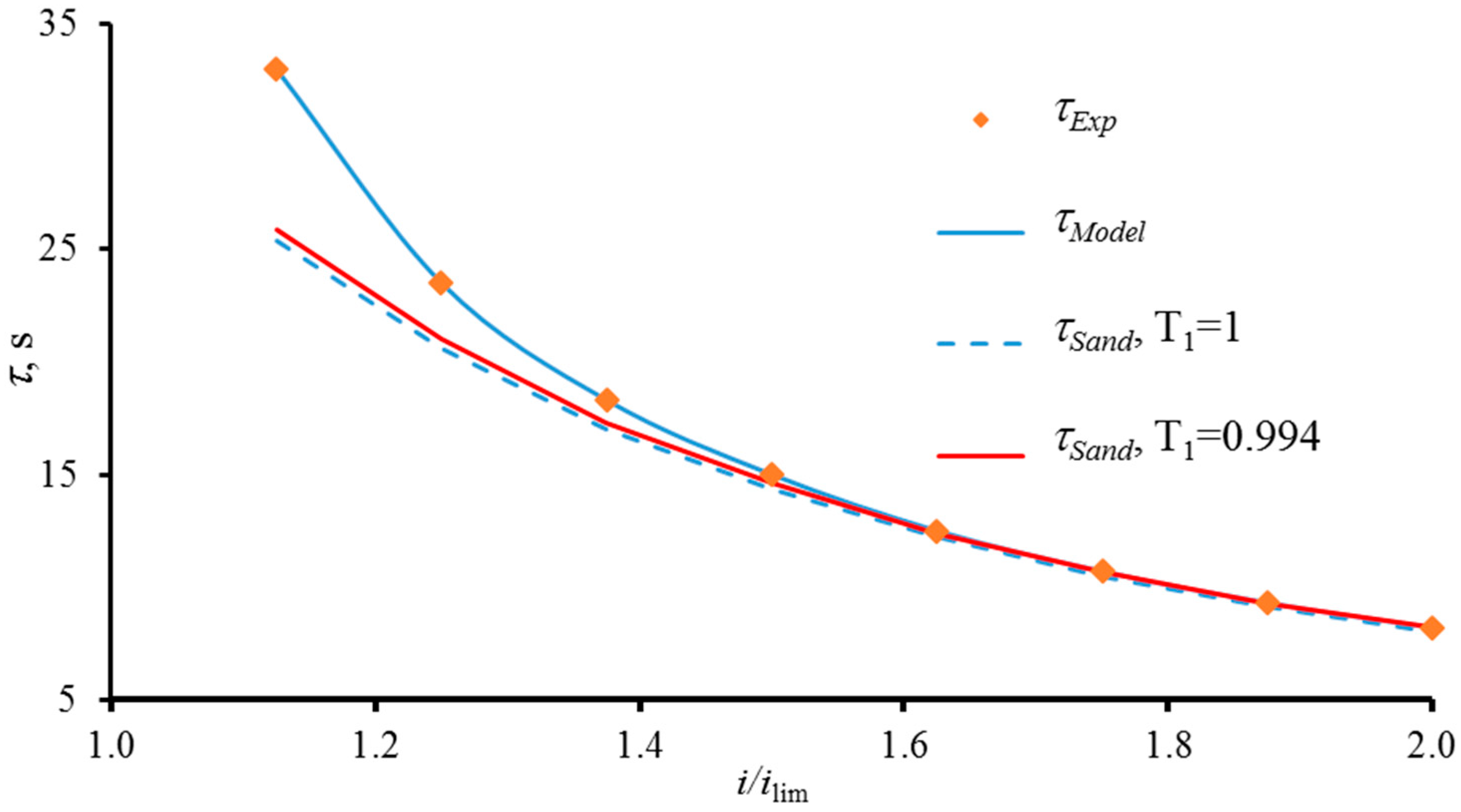
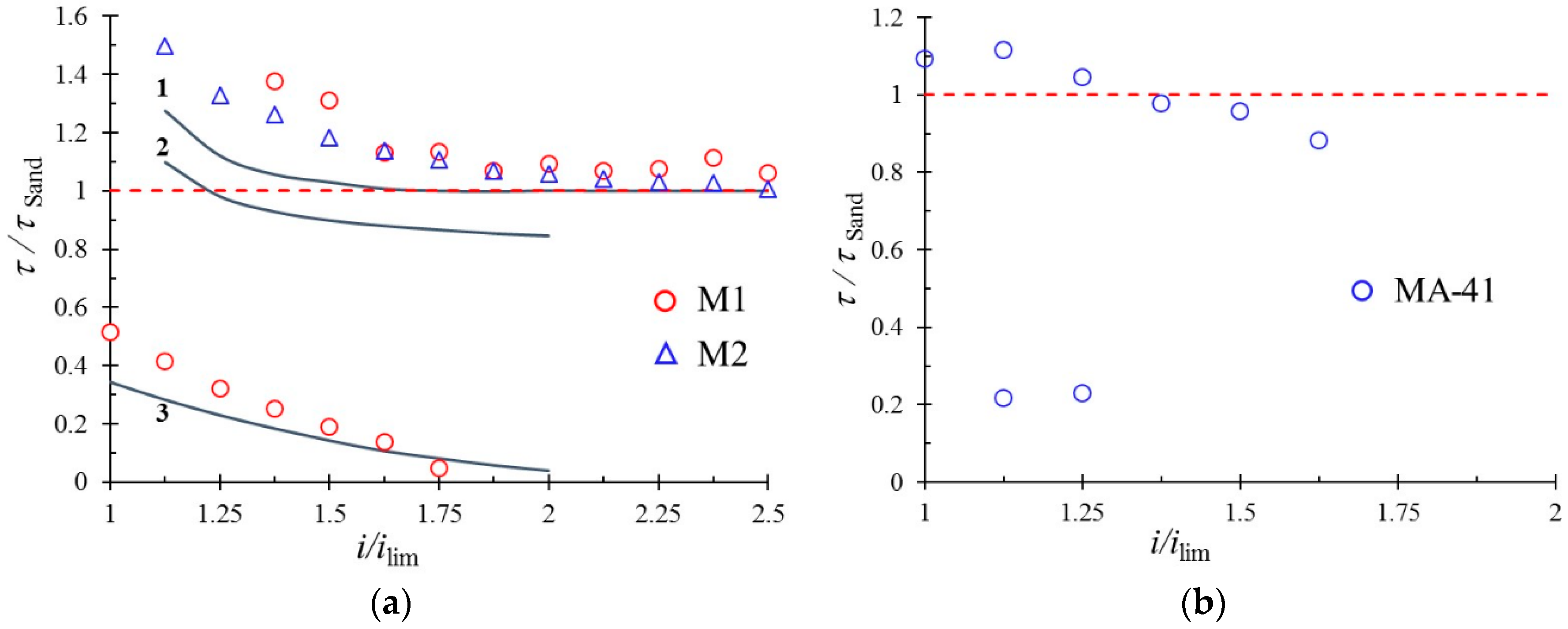
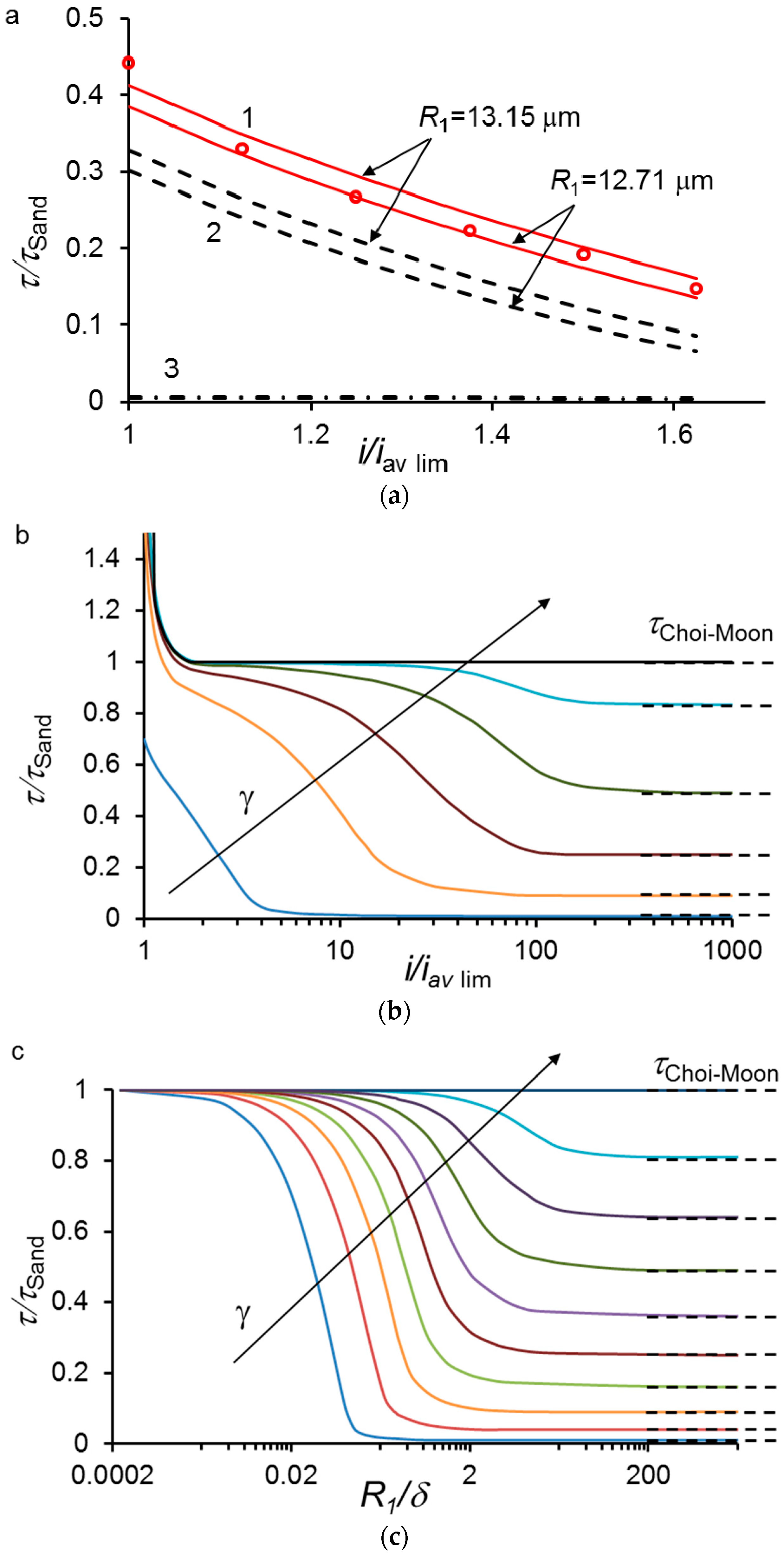
The Use of Electric Current Stream Function. Comparison with the Sand and Choi and Moon Theories

Electrochemical responses of materials having heterogeneous surface mainly depend on the parameters of surface heterogeneity [15,274,291]: on the size and shape [292,293], as well as the surface fraction [274,292,294,295,296] of conductive and nonconductive areas. Most of mathematical descriptions of ionic transport in electrochemical systems are restricted to 1D geometry [296], not relevant to a heterogeneous permselective surface.

The passage from 1D to 2D and especially 3D geometry sharply increases mathematical difficulties. Nevertheless, there are a large number of systems with permselective surface for which multidimensional effects are important: mass transfer at partially blocked electrodes [292,295], microelectrodes [297,298], proton-exchange membrane fuel cells and batteries [299]; flow electrochemical devices, such as electrolysers and electrodialysers [80,300], electrochemically heterogeneous graphene [293] or carbon nanofilaments [274], heterogeneous IEMs [15,274,291] and so forth. Development of approaches for handling multidimensional modelling of interface phenomena represents an important issue.

2D/3D mathematical description of the PD response of membrane/electrode systems is complicated since an integral condition of current intensity is needed at the permselective surface. This constitutes a problem as the current density distribution over the conductive area is not known a priori. Rubinstein et al. [274], Green and Yossifon [301,302] used the condition of uniform current density distribution on the conductive regions of membrane surface. However, this condition was not verified using another approach. The use of the electric current stream function [303] seems promising for the solution of this kind of problems, since this approach does not require any assumption about the character of current density distribution. Stream functions are widely used in fluid mechanics [304]. The main feature of this approach is that it allows calculation of the fluid velocity distribution when the volumetric flow rate is known in heterogeneous systems [305]. Another advantage is that any solution obtained with the use of stream function satisfies automatically the law of mass conservation.

Apparently, G. Taylor et al. [306] were the first who has introduced the stream function for modelling electric current across heterogeneous surface. They used the mathematical analogy between the flow of fluid and that of electric current. Later on, this approach was applied for simulation of electric current density distribution in semiconductors [307], in superconductors [308], in thin circuits [309], on the earth’s surface [310], in electromagnetic devices [311] and other systems. In membrane systems, this method was applied by Pismensky et al. [312] and Mareev et al. [303]. 3D modelling in Ref. [303] was used for describing the chronopotentiograms of a heterogeneous IEM; the results of computations were compared with experiment and with other known theories, namely, that by Sand [284], Choi and Moon [291] and Rubinstein et al. [274].

The geometry used in Ref. [303] is shown in Figure 15. A hexagonal distribution of conductive areas (the open circles in Figure 15) over the membrane surface is assumed.

The three-layer system ‘membrane + depleted DBL + enriched DBL’ adjacent to the membrane from its both sides is considered as a system of cylindrical cells (Figure 15). The membrane upper surface layer consists of a conductive disk of radius R₁ within a nonconductive ring of external radius R₂. The DBL thickness, δ, is assumed identical from both membrane sides. Using cylindrical symmetry, the system under study may be presented in two coordinates r and z.

The governing equations are the same as in the case of ED channel with heterogeneous membrane described in Section 5.3: the Nernst-Planck transport equation (without convective term), the continuity equation for ion transfer and the LEN condition. However, the time-dependent problem is considered here, that is, $\partial c_i/\partial t=-div{\overrightarrow{j}}_i\ne 0$. As in Section 5.3, the flux continuity condition at the conductive surface/solution boundaries is applied. At the non-conductive boundaries, the zero flux condition like Equation (65) is used. In galvanostatic regime, the average current density across the membrane surface, $i_{av}$, is a known parameter. It is linked with the unknown local current density as [303]:

$$i_{av}=\frac{1}{R_2}{\displaystyle \underset{0}{\overset{R_2}{\int }}{i}_z\left(r,\delta ,t\right)dr}=\frac{1}{R_2}{\displaystyle \underset{0}{\overset{R_2}{\int }}{i}_z\left(r,-d_1-d_2-\delta ,t\right)dr}=const$$

(77)

No condition on the distribution of normal current density over the conductive regions is imposed. Instead, the electric current stream function [306,312] η is introduced as follows:

$$\frac{1}{r}\frac{\partial \eta }{\partial z}=-j_r,\frac{1}{r}\frac{\partial \eta }{\partial r}=j_z$$

(78)

The charge conservation (continuity) equation in the cylindrical geometry is written in the form:

$$\frac{\partial {\rho }_e}{\partial t}=-div\overrightarrow{j}=-\left(\frac{1}{r}\frac{\partial }{\partial r}(r{j}_r)+\frac{\partial }{\partial z}{j}_z\right)=0$$

(79)

Note that Equation (79) holds, if the rate of the space charge density (${\rho }_e$) variation with time is negligible.

Equation (78) assures that Equation (79) is satisfied at any function η, if only the condition for equality of mixed derivatives of η is met.

The condition of uniform current density distribution over the conductive areas according to Refs. [274,313] is expressed as:

$${i_z(r,0+,t)|}_{r=0\dots R_1}=i_{av}/\gamma$$

(80)

However, as it is shown in Ref. [303], when integral condition, Equation (77), is applied, the current lines are concentrated within conductive areas at the boundary with the neighbour non-conductive region. The application of the uniform current density distribution, Equation (80), results in too fast decrease with time of the interfacial electrolyte concentration in the centre of conductive areas, which leads to a shorter transition time in comparison with the model [303].

The model [303] formulated above allows computation of chronopotentiograms and the transition times. As the LEN assumption and a fixed DBL thickness are used in this model, the transition time corresponds to the state where the PD tends to infinity, as in the model [269] described in Section 6.1, where the current-induced transport is implicitly taken into account.

It is known, that the transition time for heterogeneous membranes is lower than that for homogeneous ones [15,291]. However, the only mathematical description of the transition time for an electrically non-homogeneous permselective interface was made by Choi and Moon [291]. They had modified the Sand equation, Equation (76), replacing the average current density, i_av, by the local current density, $i_{local}=i_{av}/\gamma$, across the conductive areas:

$${\tau }_{Choi-Moon}=\left(\frac{\pi D}{4}\right){\left(\frac{c_{i0}{z}_{i}F}{T_i-t_i}\right)}^2\frac{{\gamma }^2}{i_{av}^2}$$

(81)

The relationship between the transition times expressed according to Sand and to Choi and Moon [291] is expressed as ${\tau }_{Choi-Moon}={\tau }_{Sand}{\gamma }^2$.

The transition time calculated using the 3D model [303] is in a good agreement with the experimental data (Figure 16a) obtained for a specially designed membrane. The substrate is a polyethylene terephthalate track-etched membrane with cylindrical randomly distributed pores with a radius of 12.93 ± 0.22 μm. The substrate was coated on one side with a Nafion^® perfluorinated resin solution of thickness d₂ about 3 μm, the Nafion^® solution filled also the pores. Thus, a membrane with a smooth homogeneous permselective surface on one side and a heterogeneous surface on the other was obtained. The circular conductive areas filled with the Nafion^® material occupy about ≈7.7% of the surface, 92.3% of the surface was non-conductive.

No fitting parameters in the model of Mareev et al. [303] are used. The curve computed for the lower bound of the range of possible radii, R₁ = 12.71 μm, is below the experimental points; that for the upper bound, R₁ = 13.15 μm, is above. The transition times calculated using the Sand equation, Equation (76), are essentially higher than the experimental ones and that calculated using the Choi-Moon equation are much lower (Figure 16a). The calculated values of τ using the 3D model [303] but under condition (80) are lower too. In fact, Equations (76) and (81) give two extreme asymptotes of the model [303]. As we mention in the previous section, the Sand Equation (76) holds, when the surface is homogeneous and the current density i > (1.5 ÷ 2)$i_{av\lim }$ [269] (Figure 16b,c). The Sand equation holds also when γ < 1 and the ratio R₁/δ is sufficiently small (Figure 16c). In this case, the concentration distribution far from the heterogeneous surface is the same as in the case of homogeneous surface. The Choi-Moon theory [291] assumes the current lines normal to the conductive surface, hence, the funnel effect [274] is not taken into account and tangential transport is considered negligible. This condition is satisfied, when R₁/δ and i are both sufficiently great (Figure 16b,c).

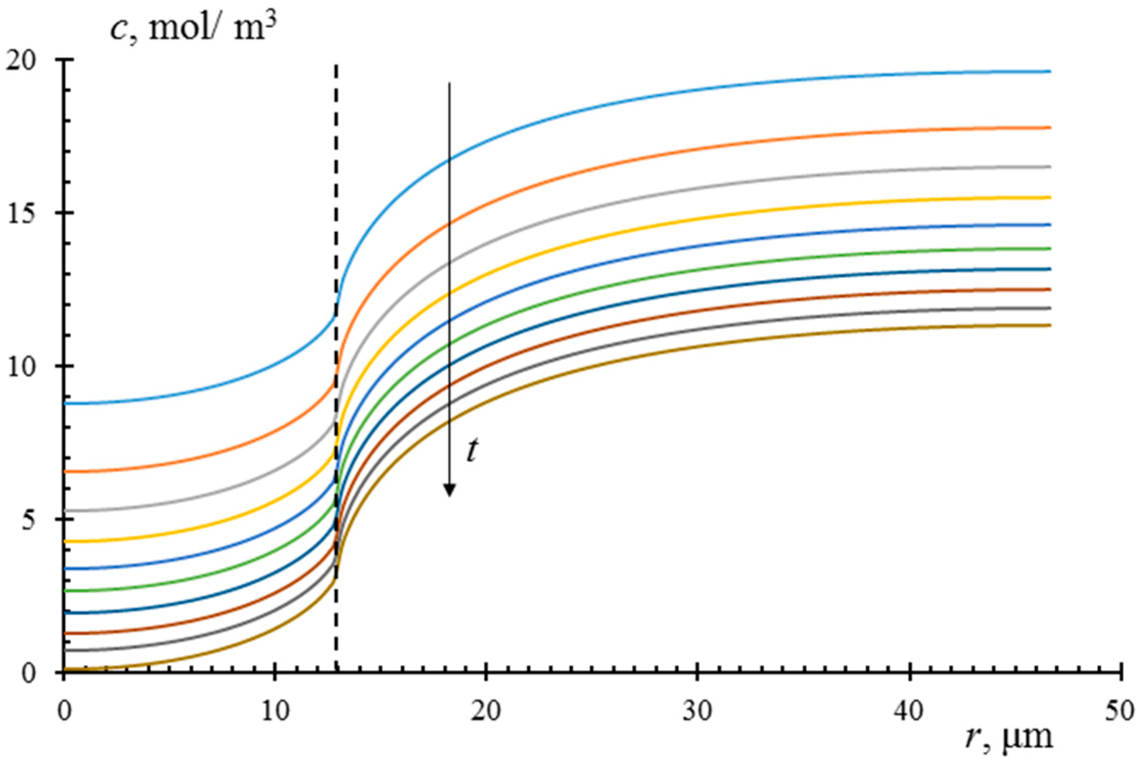
6.3. Phenomenon of Two Transition Times of Chronopotentiograms for Membranes with Heterogeneous Surface

When an electric current is applied to an IEM with electrically heterogeneous surface, the current lines are concentrated within the conductive regions. With the passage of time, the electrolyte concentration decreases first near the conductive surface regions, then the concentration changes propagate to the solution domains near the non-conducting regions (Figure 17). Tangential diffusion, which enhances the delivery of electrolyte to the surface of conductive regions occurs in this system.

The contribution of tangential diffusion is detected by appearance of two transition times in chronopotentiometry, as it was observed by Butylskii et al. [314].

The first transition time, τ₁, is attained, when the electrolyte concentration at the conductive regions of the surface becomes sufficiently low to give rise current-induced convection developed locally at the boundaries between the conductive and non-conductive regions. The second transition time, τ₂, is reached when a critically small concentration is attained at the whole membrane surface, including the conductive and non-conductive regions [314]. As the 3D model [303] predicts, when there is no current-induced convection, the electrolyte concentration remains rather elevated at the non-conductive regions, while it reaches very small values at the conductive regions (Figure 17). According to this model, only one transition time τ₁ < ${\tau }_{Sand}$ can occur in a heterogeneous membrane system if the ions in the depleted DBL are transferred by electrodiffusion solely. The decrease of concentration near the non-conductive regions may be caused by the current-induced convection, apparently electroconvection occurring as electroosmosis of the first kind [314]. Electroconvection enhances the exchange between the solution domains, which are located near the conductive and non-conductive surface regions. The onset of this enhancement (occurring at $t={\tau }_1<{\tau }_{Sand}$) reduces the rate of the PD growth, which gives the first inflection point on the chronopotentiogram. The appearance of larger electroconvective vortices, when the concentration reaches a critically small value on the entire membrane surface ($t={\tau }_2\approx {\tau }_{Sand}$), gives the second inflection point. τ₂ is close to ${\tau }_{Sand}$, since the latter event occurs also at homogeneous membrane surface. However, electroconvection occurring when the near-surface concentration is small everywhere can enhance mass transfer and slows down the rate of concentration decrease resulting in increasing τ₂ higher than ${\tau }_{Sand}$. This case is shown in Figure 18 for the M1 and M2 membranes.

The experimental values of τ₂ are essentially higher than the results of calculations for these membranes using the 3D model [303], which takes into account the electrical heterogeneity of the surface but not account for electroconvection. Note that the increase in the values of τ₂ with decreasing the $i/i_{\lim }$ ratio is due to the effect of the finite length of DBL described in Section 6.1. The behaviour of the MA-41 membrane is similar: at $i/i_{\lim }\le$ 1.25, there are two transition times. However, the $\tau /{\tau }_{Sand}$ vs. $i/i_{\lim }$ curve passes lower than the similar curves for the M2 membrane, which is apparently due to a low fraction of the conductive surface area.

7. Conclusions

In conclusion, we once again emphasize that the heterogeneity of both membrane bulk and surface plays an important role in conditioning membrane properties and enhancing their performance in electroseparation and energy production applications. The recent research shows that design of the membrane bulk affects such membrane properties as conductivity, diffusion permeability and permselectivity (mainly as related to the selective transport of ions of a certain sign of charge). An important example is the immobilization of inorganic nanoparticles in the membrane bulk, which increases membrane conductivity and permselectivity, especially at low relative humidity. Modification of membrane surface exerts a strong impact on the properties related to mass exchange between the solution and membrane surface. The use of membranes with tailored surface heterogeneity allows a significant increase of the limiting current density and overlimiting ion transport rate. It possible to talk about the formation of surfaces, self-inducing the mixing of the adjacent solution. Mathematical modelling brings a new insight into complicated transport phenomena occurring in heterogeneous systems. This deeper understanding may be very useful for the development of high-performance membranes and membrane devices. In particular, the modelling suggests that the very important factors affecting the intensity of electroconvection mixing are the size and surface fraction of the conductive/non-conductive surface regions. Numerical computations can give optimum values of these parameters. However, there is no good accordance between the computations made in different laboratories. Besides, the role of charge density and degree of hydrophilicity of surface is not yet well understood, while these parameters are also important.

Although there is a strong progress in understanding of the response of membrane performance on certain modifications of their bulk and surface, some important knowledge gaps remain. Most experiments and theoretical calculations are made for NaCl solutions and in conditions proper for laboratory tests. There are no studies on the effects of these modifications on the performance of real ED, no estimations of how these effects depend on solution concentration and forced flow velocity, what is the influence of the cell geometry, intermembrane distance, geometric shape of surface patterns, the presence of intermembrane spacers.

Even more questions remain as to the effect of modification on the membrane antifouling behaviour. The understanding of the relationships between the surface properties and antifouling resistance is rather poor. No mathematical modelling of these effects is available. The problem here is complicated by complexity of coupling between mass transport and chemical reactions, especially when the rate of these reactions is quite low. A similar situation occurs with respect to the relationship between membrane properties and the characteristics of competing transfer of ions having the same charge sign but different valence. However, given the importance of these problems for the sustainable development of society, we can expect rapid progress in this area.

References

1. Ozin, G.A.; Arsenault, A.C. Nanochemistry: A Chemical Approach to Nanomaterials. In Nanochemistry: A Chemical Approach to Nanomaterials; Royal Society of Chemistry: London, UK, 2005; p. 876. ISBN 085404664X. [Google Scholar]
2. Van Rijn, P.; Tutus, M.; Kathrein, C.; Zhu, L.; Wessling, M.; Schwaneberg, U.; Böker, A. Challenges and advances in the field of self-assembled membranes. Chem. Soc. Rev. 2013, 42, 6578–6592. [Google Scholar] [CrossRef] [PubMed]
3. Timashev, S.F. Physical Chemistry of Membrane Processes; Ellis Horwood Ltd.: New York, NY, USA, 1991; ISBN 9780136629825. [Google Scholar]
4. Nikonenko, V.V.; Yaroslavtsev, A.B.; Pourcelly, G. Ion Transfer in and Through Charged Membranes: Structure, Properties, and Theory. In Ionic Interactions in Natural and Synthetic Macromolecules; John Wiley & Sons, Inc.: Hoboken, NJ, USA, 2012; pp. 267–335. ISBN 9780470529270. [Google Scholar]
5. Kreuer, K.D.; Paddison, S.J.; Spohr, E.; Schuster, M. Transport in proton conductors for fuel-cell applications: Simulations, elementary reactions, and phenomenology. Chem. Rev. 2004, 104, 4637–4678. [Google Scholar] [CrossRef] [PubMed]
6. Strathmann, H. Ion-Exchange Membrane Separation Processes, 1st ed.; Elsevier: Amsterdam, The Netherlands, 2004; ISBN 9780444502360. [Google Scholar]
7. Xu, T. Ion exchange membranes: State of their development and perspective. J. Membr. Sci. 2005, 263, 1–29. [Google Scholar] [CrossRef]
8. Nagarale, R.K.; Gohil, G.S.; Shahi, V.K. Recent developments on ion-exchange membranes and electro-membrane processes. Adv. Colloid Interface Sci. 2006, 119, 97–130. [Google Scholar] [CrossRef] [PubMed]
9. Mizutani, Y. Review Structure of ion Exchange Membranes. J. Membr. Sci. 1990, 49, 121–144. [Google Scholar] [CrossRef]
10. Pismenskaya, N.D.; Nikonenko, V.V.; Melnik, N.A.; Shevtsova, K.A.; Belova, E.I.; Pourcelly, G.; Cot, D.; Dammak, L.; Larchet, C. Evolution with time of hydrophobicity and microrelief of a cation-exchange membrane surface and its impact on overlimiting mass transfer. J. Phys. Chem. B 2012, 116, 2145–2161. [Google Scholar] [CrossRef]
11. Mareev, S.A.; Butylskii, D.Y.; Pismenskaya, N.D.; Larchet, C.; Dammak, L.; Nikonenko, V.V. Geometric heterogeneity of homogeneous ion-exchange Neosepta membranes. J. Membr. Sci. 2018, 563, 768–776. [Google Scholar] [CrossRef]
12. Pismenskaia, N.; Sistat, P.; Huguet, P.; Nikonenko, V.; Pourcelly, G. Chronopotentiometry applied to the study of ion transfer through anion exchange membranes. J. Membr. Sci. 2004, 228, 65–76. [Google Scholar] [CrossRef]
13. Svoboda, M.; Beneš, J.; Vobecká, L.; Slouka, Z. Swelling induced structural changes of a heterogeneous cation-exchange membrane analyzed by micro-computed tomography. J. Membr. Sci. 2017, 525, 195–201. [Google Scholar] [CrossRef]
14. Vobecká, L.; Svoboda, M.; Beneš, J.; Belloň, T.T.; Slouka, Z.; Vobeckà, L.; Svoboda, M.; Beneš, J.; Belloň, T.T.; Slouka, Z.; et al. Heterogeneity of heterogeneous ion-exchange membranes investigated by chronopotentiometry and X-ray computed microtomography. J. Membr. Sci. 2018, 559, 127–137. [Google Scholar] [CrossRef]
15. Volodina, E.; Pismenskaya, N.; Nikonenko, V.; Larchet, C.; Pourcelly, G. Ion transfer across ion-exchange membranes with homogeneous and heterogeneous surfaces. J. Colloid Interface Sci. 2005, 285, 247–258. [Google Scholar] [CrossRef] [PubMed]
16. Vasil’eva, V.I.; Kranina, N.A.; Malykhin, M.D.; Akberova, E.M.; Zhiltsova, A.V. The surface inhomogeneity of ion-exchange membranes by SEM and AFM data. J. Surf. Investig. X-ray Synchrotron Neutron Tech. 2013, 7, 144–153. [Google Scholar] [CrossRef]
17. Pourcelly, G. Electrodialysis: Ion Exchange. Encycl. Sep. Sci. 2000, 2665–2675. [Google Scholar] [CrossRef]
18. Wódzki, R. ION EXCHANGE|Organic Membranes. Encycl. Sep. Sci. 2000, 1632–1639. [Google Scholar] [CrossRef]
19. Wang, W.; Fu, R.; Liu, Z.; Wang, H. Low-resistance anti-fouling ion exchange membranes fouled by organic foulants in electrodialysis. Desalination 2017, 417, 1–8. [Google Scholar] [CrossRef]
20. Sata, T. Studies on ion exchange membranes with permselectivity for specific ions in electrodialysis. J. Membr. Sci. 1994, 93, 117–135. [Google Scholar] [CrossRef]
21. Saracco, G. Transport properties of monovalent-ion-permselective membranes. Chem. Eng. Sci. 1997, 52, 3019–3031. [Google Scholar] [CrossRef]
22. Zhao, Y.; Tang, K.; Liu, H.; Van der Bruggen, B.; Sotto Díaz, A.; Shen, J.; Gao, C. An anion exchange membrane modified by alternate electro-deposition layers with enhanced monovalent selectivity. J. Membr. Sci. 2016, 520, 262–271. [Google Scholar] [CrossRef]
23. Khan, M.I.; Zheng, C.; Mondal, A.N.; Hossain, M.M.; Wu, B.; Emmanuel, K.; Wu, L.; Xu, T. Preparation of anion exchange membranes from BPPO and dimethylethanolamine for electrodialysis. Desalination 2017, 402, 10–18. [Google Scholar] [CrossRef]
24. Simons, R. Electric field effects on proton transfer between ionizable groups and water in ion exchange membranes. Electrochim. Acta 1984, 29, 151–158. [Google Scholar] [CrossRef]
25. Simons, R. A mechanism for water flow in bipolar membranes. J. Membr. Sci. 1993, 82, 65–73. [Google Scholar] [CrossRef]
26. Zabolotskii, V.I.; Shel ’deshov, N.V.; Gnusin, N.P. Dissociation of Water Molecules in Systems with Ion-exchange Membranes. Russ. Chem. Rev. 1988, 5713, 801–808. [Google Scholar] [CrossRef]
27. Strathmann, H.; Krol, J.J.; Rapp, H.J.; Eigenberger, G. Limiting current density and water dissociation in bipolar membranes. J. Membr. Sci. 1997, 125, 123–142. [Google Scholar] [CrossRef] [Green Version]
28. Scott, K. Sustainable and Green Electrochemical Science and Technology; John Wiley & Sons, Ltd.: Chichester, UK, 2017; ISBN 9781118698075. [Google Scholar]
29. Mauritz, K.A.; Moore, R.B. State of understanding of Nafion. Chem. Rev. 2004, 104, 4535–4585. [Google Scholar] [CrossRef]
30. Gebel, G. Structural evolution of water swollen perfluorosulfonated ionomers from dry membrane to solution. Polymer 2000, 41, 5829–5838. [Google Scholar] [CrossRef]
31. Helfferich, F.G. Ion Exchange; Dover Publications: Mineola, NY, USA, 1995; ISBN 0486687848. [Google Scholar]
32. Drozdov, A.D.; deClaville Christiansen, J. The effects of pH and ionic strength on equilibrium swelling of polyampholyte gels. Int. J. Solids Struct. 2017, 110–111, 192–208. [Google Scholar] [CrossRef]
33. Kozmai, A.E.; Nikonenko, V.V.; Zyryanova, S.; Pismenskaya, N.D.; Dammak, L. A simple model for the response of an anion-exchange membrane to variation in concentration and pH of bathing solution. J. Membr. Sci. 2018, 567, 127–138. [Google Scholar] [CrossRef]
34. Gierke, T.D.; Munn, G.E.; Wilson, F.C. The morphology in nafion perfluorinated membrane products, as determined by wide- and small-angle x-ray studies. J. Polym. Sci. Polym. Phys. 1981, 19, 1687–1704. [Google Scholar] [CrossRef]
35. Rubatat, L.; Rollet, A.L.; Gebel, G.; Diat, O. Evidence of elongated polymeric aggregates in Nafion. Macromolecules 2002, 35, 4050–4055. [Google Scholar] [CrossRef]
36. Kreuer, K.D. On the development of proton conducting polymer membranes for hydrogen and methanol fuel cells. J. Membr. Sci. 2001, 185, 29–39. [Google Scholar] [CrossRef]
37. Berezina, N.P.; Kononenko, N.A.; Dyomina, O.A.; Gnusin, N.P. Characterization of ion-exchange membrane materials: Properties vs structure. Adv. Colloid Interface Sci. 2008, 139, 3–28. [Google Scholar] [CrossRef] [PubMed]
38. Kononenko, N.A.; Fomenko, M.A.; Volfkovich, Y.M. Structure of perfluorinated membranes investigated by method of standard contact porosimetry. Adv. Colloid Interface Sci. 2015, 222, 425–435. [Google Scholar] [CrossRef] [PubMed]
39. Kononenko, N.; Nikonenko, V.; Grande, D.; Larchet, C.; Dammak, L.; Fomenko, M.; Volfkovich, Y. Porous structure of ion exchange membranes investigated by various techniques. Adv. Colloid Interface Sci. 2017, 246, 196–216. [Google Scholar] [CrossRef] [PubMed]
40. Divisek, J.; Eikerling, M.; Mazin, V.; Schmitz, H.; Stimming, U.; Volfkovich, Y.M. A Study of Capillary Porous Structure and Sorption Properties of Nafion Proton-Exchange Membranes Swollen in Water. J. Electrochem. Soc. 1998, 145, 2677. [Google Scholar] [CrossRef]
41. Bryk, M.T.; Zabolotskii, V.I.; Atamanenko, I.D.; Dvorkina, G.A. Structural inhomogeneity of ion-exchange membranes in swelling state andmethods of its investigations. Sov. J. Water Chem. Technol. 1989, 11, 14. [Google Scholar]
42. Berezina, N.P.; Shkirskaya, S.A.; Kolechko, M.V.; Popova, O.V.; Senchikhin, I.N.; Roldugin, V.I. Barrier effects of polyaniline layer in surface modified MF-4SK/Polyaniline membranes. Russ. J. Electrochem. 2011, 47, 995–1005. [Google Scholar] [CrossRef]
43. Haubold, H.G.; Vad, T.; Jungbluth, H.; Hiller, P. Nano structure of NAFION: A SAXS study. Electrochim. Acta 2001, 46, 1559–1563. [Google Scholar] [CrossRef]
44. Kornyshev, A.A.; Kuznetsov, A.M.; Spohr, E.; Ulstrup, J. Kinetics of proton transport in water. J. Phys. Chem. B 2003, 107, 3351–3366. [Google Scholar] [CrossRef]
45. Paddison, S.J. Proton Conduction Mechanisms at Low Degrees of Hydration in Sulfonic Acid–Based Polymer Electrolyte Membranes. Annu. Rev. Mater. Res. 2003, 33, 289–319. [Google Scholar] [CrossRef]
46. Larchet, C.; Nouri, S.; Auclair, B.; Dammak, L.; Nikonenko, V. Application of chronopotentiometry to determine the thickness of diffusion layer adjacent to an ion-exchange membrane under natural convection. Adv. Colloid Interface Sci. 2008, 139, 45–61. [Google Scholar] [CrossRef]
47. Kamcev, J.; Paul, D.R.; Freeman, B.D. Ion activity coefficients in ion exchange polymers: Applicability of Manning’s counterion condensation theory. Macromolecules 2015, 48, 8011–8024. [Google Scholar] [CrossRef]
48. Kamcev, J.; Galizia, M.; Benedetti, F.M.; Jang, E.S.; Paul, D.R.; Freeman, B.D.; Manning, G.S. Partitioning of mobile ions between ion exchange polymers and aqueous salt solutions: Importance of counter-ion condensation. Phys. Chem. Chem. Phys. 2016, 18, 6021–6031. [Google Scholar] [CrossRef]
49. Kamcev, J.; Paul, D.R.; Freeman, B.D. Effect of fixed charge group concentration on equilibrium ion sorption in ion exchange membranes. J. Mater. Chem. A 2017, 5, 4638–4650. [Google Scholar] [CrossRef]
50. Mumford, D. Selected Papers, 1st ed.; Springer: New York, NY, USA; Copenhagen, Denmark, 2004; ISBN 978-1-4419-1936-6. [Google Scholar]
51. Manning, G.S. Limiting Laws and Counterion Condensation in Polyelectrolyte Solutions I. Colligative Properties. J. Chem. Phys. 1969, 51, 924–933. [Google Scholar] [CrossRef]
52. Manning, G.S. The molecular theory of polyelectrolyte solutions with applications to the electrostatic properties of polynucleotides. Q. Rev. Biophys. 1978, 11, 179. [Google Scholar] [CrossRef] [PubMed]
53. Muthukumar, M. Polymer Translocation, 1st ed.; CRC Press: Boca Raton, FL, USA, 2011; ISBN 9781420075175. [Google Scholar]
54. Zabolotskii, V.V.; Nikonenko, V.V. Ion Transport in Membranes (in Russian); Nauka: Moscow, Russia, 1996; ISBN 5-02-001677-2. [Google Scholar]
55. Lakshminarayanaiah, N. Transport Phenomena in Membranes; Acad. Press: New York, NY, USA, 1969; ISBN 9780124342507. [Google Scholar]
56. Kontturi, K.; Murtomäki, L.; Manzanares, J.A. Ionic Transport Processes: In Electrochemistry and Membrane Science; Oxford University Press: Oxford, UK, 2008; ISBN 9780198719991. [Google Scholar]
57. Tanaka, Y. Ion Exchange Membranes, Volume 12 2nd Edition. In Fundamentals and Applications; Elsevier Science: Amsterdam, The Netherlands, 2015; p. 522. ISBN 9780444633194. [Google Scholar]
58. Yaroslavtsev, A.B.; Nikonenko, V.V.; Zabolotsky, V.I. Ion transfer in ion-exchange and membrane materials. Russ. Chem. Rev. 2003, 72, 393–421. [Google Scholar] [CrossRef]
59. Weber, A.Z.; Newman, J. A combination model for macroscopic transport in polymer-electrolyte membranes. Top. Appl. Phys. 2009, 113, 157–198. [Google Scholar]
60. Wang, C.Y. Fundamental models for fuel cell engineering. Chem. Rev. 2004, 104, 4727–4765. [Google Scholar] [CrossRef]
61. Kondepudi, D.; Prigogine, I. Modern Thermodynamics: From Heat Engines to Dissipative Structures, 2nd ed.; John Wiley: Hoboken, NJ, USA, 2014; Volume 9781118371, ISBN 9781118698723. [Google Scholar]
62. Spiegler, K.S. Transport processes in ionic membranes. Trans. Faraday Soc. 1958, 54, 1408–1428. [Google Scholar] [CrossRef]
63. Zabolotsky, V.I.; Nikonenko, V.V. Effect of structural membrane inhomogeneity on transport properties. J. Membr. Sci. 1993, 79, 181–198. [Google Scholar] [CrossRef]
64. Kedem, O.; Katchalsky, A. A physical interpretation of the phenomenological coefficients of membrane permeability. J. Gen. Physiol. 1961, 45, 143–179. [Google Scholar] [CrossRef] [PubMed]
65. Narȩbska, A.; Koter, S.; Kujawski, W. Ions and water transport across charged nafion membranes. Irreversible thermodynamics approach. Desalination 1984, 51, 3–17. [Google Scholar] [CrossRef]
66. Spiegler, K.S.; Kedem, O. Thermodynamics of hyperfiltration (reverse osmosis): Criteria for efficient membranes. Desalination 1966, 1, 311–326. [Google Scholar] [CrossRef]
67. Auclair, B.; Nikonenko, V.; Larchet, C.; Métayer, M.; Dammak, L. Correlation between transport parameters of ion-exchange membranes. J. Membr. Sci. 2001, 195, 89–102. [Google Scholar] [CrossRef]
68. Kedem, O.; Katchalsky, A. Permeability of composite membranes Part 1—Electric current, volume flow and flow of solute through membranes. Trans. Faraday Soc. 1963, 59, 1918–1930. [Google Scholar] [CrossRef]
69. Meares, P. Coupling of ion and water fluxes in synthetic membranes. J. Membr. Sci. 1981, 8, 295–307. [Google Scholar] [CrossRef]
70. Mason, E.A.; Lonsdale, H.K. Statistical-mechanical theory of membrane transport. J. Membr. Sci. 1990, 51, 1–81. [Google Scholar] [CrossRef]
71. Koter, S.; Kujawski, W.; Koter, I. Importance of the cross-effects in the transport through ion-exchange membranes. J. Membr. Sci. 2007, 297, 226–235. [Google Scholar] [CrossRef]
72. Kedem, O.; Perry, M. A simple procedure for estimating ion coupling from conventional transport coefficients. J. Membr. Sci. 1983, 14, 249–262. [Google Scholar] [CrossRef]
73. Narȩbska, A.; Koter, S. Permselectivity of ion-exchange membranes in operating systems. Irreversible thermodynamics treatment. Electrochim. Acta 1993, 38, 815–819. [Google Scholar] [CrossRef]
74. Gnusin, N.P.; Berezina, N.P.; Kononenko, N.A.; Dyomina, O.A. Transport structural parameters to characterize ion exchange membranes. J. Membr. Sci. 2004, 243, 301–310. [Google Scholar] [CrossRef]
75. Larchet, C.; Auclair, B.; Nikonenko, V. Approximate evaluation of water transport number in ion-exchange membranes. Electrochim. Acta 2004, 49, 1711–1717. [Google Scholar] [CrossRef]
76. Larchet, C.; Dammak, L.; Auclair, B.; Parchikov, S.; Nikonenko, V. A simplified procedure for ion-exchange membrane characterisation. New J. Chem. 2004, 28, 1260. [Google Scholar] [CrossRef]
77. Paterson, R.; Gardner, C.R. Comparison of the transport properties of normal and expanded forms of a cation-exchange membrane by use of an irreversible thermodynamic approach. Part I. Membranes in the sodium form in 0·1 M-sodium chloride. J. Chem. Soc. A 1971, 2254–2261. [Google Scholar] [CrossRef]
78. Robinson, R.A.; Stokes, R.H. Electrolyte Solutions, 2nd ed.; Butterworths: London, UK, 2002; ISBN 0-486-42225-9. [Google Scholar]
79. Lebrun, L.; Da Silva, E.; Pourcelly, G.; Métayer, M. Elaboration and characterisation of ion-exchange films used in the fabrication of bipolar membranes. J. Membr. Sci. 2003, 227, 95–111. [Google Scholar] [CrossRef]
80. Newman, J.S.; Thomas-Alyea, K.E. Electrochemical Systems; John Wiley & Sons, Inc.: Hoboken, NJ, USA, 2004; ISBN 3175723993. [Google Scholar]
81. Zaltzman, B.; Rubinstein, I. Electro-osmotic slip and electroconvective instability. J. Fluid Mech. 2007, 579, 173–226. [Google Scholar] [CrossRef]
82. Chu, K.T.; Bazant, M.Z. Electrochemical Thin Films at and above the Classical Limiting Current. SIAM J. Appl. Math. 2005, 65, 1485–1505. [Google Scholar] [CrossRef] [Green Version]
83. Urtenov, M.A.K.; Kirillova, E.V.; Seidova, N.M.; Nikonenko, V.V. Decoupling of the Nernst-Planck and Poisson equations. Application to a membrane system at overlimiting currents. J. Phys. Chem. B 2007, 111, 14208–14222. [Google Scholar] [CrossRef]
84. Kamcev, J.; Sujanani, R.; Jang, E.S.; Yan, N.; Moe, N.; Paul, D.R.; Freeman, B.D. Salt concentration dependence of ionic conductivity in ion exchange membranes. J. Membr. Sci. 2018, 547, 123–133. [Google Scholar] [CrossRef]
85. Wijmans, J.G.; Baker, R.W. The solution-diffusion model: A review. J. Membr. Sci. 1995, 107, 1–21. [Google Scholar] [CrossRef]
86. Baker, R.W. Membrane Technology and Applications, 3rd ed.; John Wiley and Sons Ltd.: Hoboken, NJ, USA, 2012; ISBN 9780470743720. [Google Scholar]
87. Paul, D.R. Reformulation of the solution-diffusion theory of reverse osmosis. J. Membr. Sci. 2004, 241, 371–386. [Google Scholar] [CrossRef]
88. Kamcev, J.; Paul, D.R.; Manning, G.S.; Freeman, B.D. Accounting for frame of reference and thermodynamic non-idealities when calculating salt diffusion coefficients in ion exchange membranes. J. Membr. Sci. 2017, 537, 396–406. [Google Scholar] [CrossRef]
89. Kamcev, J.; Paul, D.R.; Manning, G.S.; Freeman, B.D. Predicting salt permeability coefficients in highly swollen, highly charged ion exchange membranes. ACS Appl. Mater. Interfaces 2017, 9, 4044–4056. [Google Scholar] [CrossRef] [PubMed]
90. Yaroshchuk, A.E.; Dukhin, S.S. Phenomenological theory of reverse osmosis in macroscopically homogeneous membranes and its specification for the capillary space-charge model. J. Membr. Sci. 1993, 79, 133–158. [Google Scholar] [CrossRef]
91. Choy, T.C. Effective Medium Theory: Principles and Applications; Oxford University Press: Oxford, UK, 2015; ISBN 0198518927. [Google Scholar]
92. Kjelstrup, S.; Bedeaux, D. Non-Equilibrium Thermodynamics of Heterogeneous Systems; World Scientific Publishing Co. Pte. Ltd.: Singapore, 2008; ISBN 9789812779137. [Google Scholar]
93. Galama, A.H.; Post, J.W.; Hamelers, H.V.M.; Nikonenko, V.V.; Biesheuvel, P.M. On the origin of the membrane potential arising across densely charged ion exchange membranes: How well does the Teorell-Meyer-Sievers theory work? J. Membr. Sci. Res. 2016, 2, 128–140. [Google Scholar] [CrossRef]
94. Geise, G.M.; Paul, D.R.; Freeman, B.D. Fundamental water and salt transport properties of polymeric materials. Prog. Polym. Sci. 2014, 39, 1–42. [Google Scholar] [CrossRef]
95. Bandini, S.; Bruni, L. Transport Phenomena in Nanofiltration Membranes. In Comprehensive Membrane Science and Engineering; Elsevier Science: Amsterdam, The Netherlands, 2010; pp. 1–21. ISBN 9780080932507. [Google Scholar]
96. Jonsson, G.; Macedonio, F. Fundamentals in Reverse Osmosis. In Comprehensive Membrane Science and Engineering; Elsevier Science: Amsterdam, The Netherlands, 2010; Volume 2, pp. 1–22. ISBN 9780080932507. [Google Scholar]
97. Caputo, M.; Cametti, C. Diffusion with memory in two cases of biological interest. J. Theor. Biol. 2008, 254, 697–703. [Google Scholar] [CrossRef]
98. Tedesco, M.; Hamelers, H.V.M.; Biesheuvel, P.M. Nernst-Planck transport theory for (reverse) electrodialysis: II. Effect of water transport through ion-exchange membranes. J. Membr. Sci. 2017, 531, 172–182. [Google Scholar] [CrossRef] [Green Version]
99. Ding, M.; Ghoufi, A.; Szymczyk, A. Molecular simulations of polyamide reverse osmosis membranes. Desalination 2014, 343, 48–53. [Google Scholar] [CrossRef]
100. Ding, M.; Szymczyk, A.; Ghoufi, A. On the structure and rejection of ions by a polyamide membrane in pressure-driven molecular dynamics simulations. Desalination 2015, 368, 76–80. [Google Scholar] [CrossRef]
101. Ding, M.; Szymczyk, A.; Goujon, F.; Soldera, A.; Ghoufi, A. Structure and dynamics of water confined in a polyamide reverse-osmosis membrane: A molecular-simulation study. J. Membr. Sci. 2014, 458, 236–244. [Google Scholar] [CrossRef]
102. Ding, M.; Szymczyk, A.; Ghoufi, A. Hydration of a polyamide reverse-osmosis membrane. J. Membr. Sci. 2016, 501, 248–253. [Google Scholar] [CrossRef]
103. Teorell, T. An Attempt to Formulate a Quantitative Theory of Membrane Permeability. Exp. Biol. Med. 1935, 33, 282–285. [Google Scholar] [CrossRef]
104. Meyer, K.H.; Sievers, J.F. La perméabilité des membranes I. Théorie de la perméabilité ionique. Helv. Chim. Acta 1936, 19, 649–664. [Google Scholar] [CrossRef]
105. Verbrugge, M.W.; Pintauro, P.N. Transport Models for Ion-Exchange Membranes; Springer: Boston, MA, USA, 1989; pp. 1–67. [Google Scholar]
106. Miller, D.G. Application of Irreversible Thermodynamics to Electrolyte Solutions. I. Determination of Ionic Transport Coefficients lij for Isothermal Vector Transport Processes in Binary Electrolyte Systems. J. Phys. Chem. 1966, 70, 2639–2659. [Google Scholar] [CrossRef]
107. Pitzer, K.S. Thermodynamic model for aqueous solutions of liquid-like density. Rev. Mineral. 1987, 81. [Google Scholar] [CrossRef]
108. Wright, M.R. An Introduction to Aqueous Electrolyte Solutions; John Wiley: Hoboken, NJ, USA, 2007; ISBN 9780470842935. [Google Scholar]
109. Manning, G.S. Polyelectrolytes. Annu. Rev. Phys. Chem. 1972, 23, 117–140. [Google Scholar] [CrossRef]
110. Manning, G.S. Counterion binding in polyelectrolyte theory. Acc. Chem. Res. 1979, 12, 443–449. [Google Scholar] [CrossRef]
111. Hiemenz, P.C.; Lodge, T.P. Polymer Chemistry, 2nd ed.; CRC Press: Boca Raton, Fl, USA, 2007; ISBN 1574447793. [Google Scholar]
112. Tanaka, Y. Chapter 4 Theory of Teorell, Meyer and Sievers (TMS Theory). Membr. Sci. Technol. 2007, 12, 59–66. [Google Scholar] [CrossRef]
113. Wang, X.-L.; Tsuru, T.; Nakao, S.-I.; Kimura, S. Electrolyte transport through nanofiltration membranes by the space-charge model and the comparison with Teorell-Meyer-Sievers model. J. Membr. Sci. 1995, 103, 117–133. [Google Scholar] [CrossRef]
114. Filippov, A.N.; Starov, V.M.; Kononenko, N.A.; Berezina, N.P. Asymmetry of diffusion permeability of bi-layer membranes. Adv. Colloid Interface Sci. 2008, 139, 29–44. [Google Scholar] [CrossRef] [PubMed]
115. Filippov, A.N.; Safronova, E.Y.; Yaroslavtsev, A.B. Theoretical and experimental investigation of diffusion permeability of hybrid MF-4SC membranes with silica nanoparticles. J. Membr. Sci. 2014, 471, 110–117. [Google Scholar] [CrossRef]
116. Filippov, A.; Khanukaeva, D.; Afonin, D.; Skorikova, G.; Ivanov, E.; Vinokurov, V.; Lvov, Y. Transport Properties of Novel Hybrid Cation-Exchange Membranes on the Base of MF-4SC and Halloysite Nanotubes. J. Mater. Sci. Chem. Eng. 2015, 3, 58–65. [Google Scholar] [CrossRef]
117. Filippov, A.; Afonin, D.; Kononenko, N.; Lvov, Y.; Vinokurov, V. New approach to characterization of hybrid nanocomposites. Colloids Surf. A Physicochem. Eng. Asp. 2017, 521, 251–259. [Google Scholar] [CrossRef]
118. Fíla, V.; Bouzek, K. A mathematical model of multiple ion transport across an ion-selective membrane under current load conditions. J. Appl. Electrochem. 2003, 33, 675–684. [Google Scholar] [CrossRef]
119. Fíla, V.; Bouzek, K. The effect of convection in the external diffusion layer on the results of a mathematical model of multiple ion transport across an ion-selective membrane. J. Appl. Electrochem. 2008, 38, 1241–1252. [Google Scholar] [CrossRef]
120. Sokirko, A.V.; Manzanares, J.A.; Pellicer, J. The Permselectivity of Membrane Systems with an Inhomogeneous Distribution of Fixed Charge Groups. J. Colloid Interface Sci. 1994, 168, 32–39. [Google Scholar] [CrossRef]
121. Moya, A.A.; Moleón, J.A. Study of the electrical properties of bi-layer ion-exchange membrane systems. J. Electroanal. Chem. 2010, 647, 53–59. [Google Scholar] [CrossRef]
122. Balannec, B.; Ghoufi, A.; Szymczyk, A. Nanofiltration performance of conical and hourglass nanopores. J. Membr. Sci. 2018, 552, 336–340. [Google Scholar] [CrossRef]
123. Dubinin, M.M. Surface and Porosity of Adsorbents. Russ. Chem. Rev. 1982, 51, 605–611. [Google Scholar] [CrossRef]
124. Sélégny, E.; Boyd, G.; Gregor, H.P. Charged Gels and Membranes: Part I; Springer Science & Business Media: Berlin, Germany, 1976; ISBN 9401014647. [Google Scholar]
125. Mafé, S.; Manzanares, J.A.; Ramirez, P. Modeling of surface vs. bulk ionic conductivity in fixed charge membranes. Phys. Chem. Chem. Phys. 2003, 5, 376–383. [Google Scholar] [CrossRef]
126. Rojo, A.G.; Roman, H.E. Effective-medium approach for the conductivity of dispersed ionic conductors. Phys. Rev. B 1988, 37, 3696–3698. [Google Scholar] [CrossRef]
127. Duan, H.L.; Karihaloo, B.L.; Wang, J.; Yi, X. Effective conductivities of heterogeneous media containing multiple inclusions with various spatial distributions. Phys. Rev. B 2006, 73, 174203. [Google Scholar] [CrossRef]
128. Starov, V.M.; Zhdanov, V.G. Effective properties of suspensions/emulsions, porous and composite materials. Adv. Colloid Interface Sci. 2008, 137, 2–19. [Google Scholar] [CrossRef] [PubMed]
129. Pal, R. Thermal conductivity of three-component composites of core-shell particles. Mater. Sci. Eng. A 2008, 498, 135–141. [Google Scholar] [CrossRef]
130. Zhdanov, M. Generalized effective-medium theory of induced polarization. Geophysics 2008, 73, F197–F211. [Google Scholar] [CrossRef]
131. Vasin, S.I.; Filippov, A.N.; Starov, V.M. Hydrodynamic permeability of membranes built up by particles covered by porous shells: Cell models. Adv. Colloid Interface Sci. 2008, 139, 83–96. [Google Scholar] [CrossRef]
132. Maxwell, J.C. A Treatise on Electricity and Magnetism V2 (1873) (Clarendon Press Series); Clarendon: Oxford, UK, 1873; ISBN 978-0548642573. [Google Scholar]
133. Mackie, J.S.; Meares, P. The Diffusion of Electrolytes in a Cation-Exchange Resin Membrane. I. Theoretical. Proc. R. Soc. A Math. Phys. Eng. Sci. 1955, 232, 498–509. [Google Scholar] [CrossRef]
134. Wódzki, R.; Narebska, A. Composition and structure of cation permselective membranes II. Multilayer electrochemical model. Angew. Makromol. Chem. 1980, 88, 149–163. [Google Scholar] [CrossRef]
135. Gnusin, N.P.; Zabolotsky, V.I.; Meshechkov, A.I. Development of the generalized conductance principle to the description of transfer phenomena in disperse systems under the acting of different forces. Russ. J. Phys. Chem. 1980, 54, 1518–1522. [Google Scholar]
136. Hsu, W.Y.; Gierke, T.D.; Molnar, C.J. Morphological effects on the physical properties of polymer composites. Macromolecules 1983, 16, 1945–1947. [Google Scholar] [CrossRef]
137. Belaid, N.; Ngom, B.; Dammak, L.; Larchet, C.; Auclair, B. Conductivité membranaire: Interprétation et exploitation selon le modèle à solution interstitielle hétérogène. Eur. Polym. J. 1999, 35, 879–897. [Google Scholar] [CrossRef]
138. Elattar, A.; Elmidaoui, A.; Pismenskaia, N.; Gavach, C.; Pourcelly, G. Comparison of transport properties of monovalent anions through anion-exchange membranes. J. Membr. Sci. 1998, 143, 249–261. [Google Scholar] [CrossRef]
139. Gohil, G.S.; Shahi, V.K.; Rangarajan, R. Comparative studies on electrochemical characterization of homogeneous and heterogeneous type of ion-exchange membranes. J. Membr. Sci. 2004, 240, 211–219. [Google Scholar] [CrossRef]
140. Xu, T.W.; Li, Y.; Wu, L.; Yang, W.H. A simple evaluation of microstructure and transport parameters of ion-exchange membranes from conductivity measurements. Sep. Purif. Technol. 2008, 60, 73–80. [Google Scholar] [CrossRef]
141. Sedkaoui, Y.; Szymczyk, A.; Lounici, H.; Arous, O. A new lateral method for characterizing the electrical conductivity of ion-exchange membranes. J. Membr. Sci. 2016, 507, 34–42. [Google Scholar] [CrossRef] [Green Version]
142. Vyas, P.; Ray, P.; Adhikary, S.; Shah, B.; Rangarajan, R. Studies of the effect of variation of blend ratio on permselectivity and heterogeneity of ion-exchange membranes. J. Colloid Interface Sci. 2003, 257, 127–134. [Google Scholar] [CrossRef]
143. Le, X.T.; Bui, T.H.; Viel, P.; Berthelot, T.; Palacin, S. On the structure-properties relationship of the AMV anion exchange membrane. J. Membr. Sci. 2009, 340, 133–140. [Google Scholar] [CrossRef]
144. Le, X.T. Permselectivity and microstructure of anion exchange membranes. J. Colloid Interface Sci. 2008, 325, 215–222. [Google Scholar] [CrossRef]
145. Berezina, N.; Gnusin, N.; Dyomina, O.; Timofeyev, S. Water electrotransport in membrane systems. Experiment and model description. J. Membr. Sci. 1994, 86, 207–229. [Google Scholar] [CrossRef]
146. Tuan, L.X.; Buess-Herman, C. Study of water content and microheterogeneity of CMS cation exchange membrane. Chem. Phys. Lett. 2007, 434, 49–55. [Google Scholar] [CrossRef]
147. Pismenskaya, N.D.; Nevakshenova, E.E.; Nikonenko, V.V. Using a Single Set of Structural and Kinetic Parameters of the Microheterogeneous Model to Describe the Sorption and Kinetic Properties of Ion-Exchange Membranes. Pet. Chem. 2018, 58, 465–473. [Google Scholar] [CrossRef]
148. Zabolotskii, V.I.; Nikonenko, V.V.; Kostenko, O.N.; Elnikova, L.F. Analysis of ion-exchange membranes using microheterogeneous models. Russ. J. Phys. Chem. 1993, 67, 2423–2427. [Google Scholar]
149. Tuan, L.X.; Mertens, D.; Buess-Herman, C. The two-phase model of structure microheterogeneity revisited by the study of the CMS cation exchange membrane. Desalination 2009, 240, 351–357. [Google Scholar] [CrossRef]
150. Geise, G.M.; Falcon, L.P.; Freeman, B.D.; Paul, D.R. Sodium chloride sorption in sulfonated polymers for membrane applications. J. Membr. Sci. 2012, 423–424, 195–208. [Google Scholar] [CrossRef]
151. Huguet, P.; Kiva, T.; Noguera, O.; Sistat, P.; Nikonenko, V. The crossed interdiffusion of sodium nitrate and sulfate through an anion exchange membrane, as studied by Raman spectroscopy. New J. Chem. 2005, 29, 955. [Google Scholar] [CrossRef]
152. Zabolotsky, V.I.; Lebedev, K.A.; Nikonenko, V.V.; Shudrenko, A.A. Identification of a microheterogeneous model for a heterogeneous membrane. Russ. J. Electrochem. 1993, 29, 811–816. [Google Scholar]
153. Karpenko-Jereb, L.V.; Berezina, N.P. Determination of structural, selective, electrokinetic and percolation characteristics of ion-exchange membranes from conductive data. Desalination 2009, 245, 587–596. [Google Scholar] [CrossRef]
154. Lee, H.-J.; Hong, M.-K.; Han, S.-D.; Moon, S.-H. Influence of the heterogeneous structure on the electrochemical properties of anion exchange membranes. J. Membr. Sci. 2008, 320, 549–555. [Google Scholar] [CrossRef]
155. Pismenskaya, N.D.; Belova, E.I.; Nikonenko, V.V.; Larchet, C. Electrical conductivity of cation-and anion-exchange membranes in ampholyte solutions. Russ. J. Electrochem. 2008, 44, 1285–1291. [Google Scholar] [CrossRef]
156. Volfkovich, Y.; Filippov, A.; Bagotsky, V. Structural Properties of Porous Materials and Powders Used in Different Fields of Science and Technology; Springer: London, UK, 2014; ISBN 978-1-4471-6376-3. [Google Scholar]
157. Chaabane, L.; Bulvestre, G.; Larchet, C.; Nikonenko, V.; Deslouis, C.; Takenouti, H. The influence of absorbed methanol on the swelling and conductivity properties of cation-exchange membranes: Evaluation of nanostructure parameters. J. Membr. Sci. 2008, 323, 167–175. [Google Scholar] [CrossRef]
158. Choi, J.-H.H.; Kim, S.-H.H.; Moon, S.-H.H. Heterogeneity of ion-exchange membranes: The effects of membrane heterogeneity on transport properties. J. Colloid Interface Sci. 2001, 241, 120–126. [Google Scholar] [CrossRef] [PubMed]
159. Tuan, L.X.; Verbanck, M.; Buess-Herman, C.; Hurwitz, H.D. Properties of CMV cation exchange membranes in sulfuric acid media. J. Membr. Sci. 2006, 284, 67–78. [Google Scholar] [CrossRef]
160. Villaluenga, J.P.G.; Barragán, V.M.; Izquierdo-Gil, M.A.; Godino, M.P.; Seoane, B.; Ruiz-Bauzá, C. Comparative study of liquid uptake and permeation characteristics of sulfonated cation-exchange membranes in water and methanol. J. Membr. Sci. 2008, 323, 421–427. [Google Scholar] [CrossRef]
161. Kumar, M.; Singh, S.; Shahi, V.K. Cross-Linked Poly(vinyl alcohol)−Poly(acrylonitrile-co-2-dimethylamino ethylmethacrylate) Based Anion-Exchange Membranes in Aqueous Media. J. Phys. Chem. B 2010, 114, 198–206. [Google Scholar] [CrossRef] [PubMed]
162. Alberti, G.; Casciola, M. Solid state protonic conductors, present main applications and future prospects. Solid State Ionics 2001, 145, 3–16. [Google Scholar] [CrossRef]
163. Adjemian, K.T.; Lee, S.J.; Srinivasan, S.; Benziger, J.; Bocarsly, A.B. Silicon Oxide Nafion Composite Membranes for Proton-Exchange Membrane Fuel Cell Operation at 80–140°C. J. Electrochem. Soc. 2002, 149, A256–A261. [Google Scholar] [CrossRef]
164. Jalani, N.H.; Dunn, K.; Datta, R. Synthesis and characterization of Nafion®-MO2 (M = Zr, Si, Ti) nanocomposite membranes for higher temperature PEM fuel cells. Electrochim. Acta 2005, 51, 553–560. [Google Scholar] [CrossRef]
165. Pereira, F.; Vallé, K.; Belleville, P.; Morin, A.; Lambert, S.; Sanchez, C. Advanced Mesostructured Hybrid Silica−Nafion Membranes for High-Performance PEM Fuel Cell. Chem. Mater. 2008, 20, 1710–1718. [Google Scholar] [CrossRef]
166. Safronova, E.Y.; Volkov, V.I.; Yaroslavtsev, A.B. Ion mobility and conductivity of hybrid ion-exchange membranes incorporating inorganic nanoparticles. Solid State Ion. 2011, 188, 129–131. [Google Scholar] [CrossRef]
167. Gerasimova, E.; Safronova, E.; Ukshe, A.; Dobrovolsky, Y.; Yaroslavtsev, A. Electrocatalytic and transport properties of hybrid Nafion® membranes doped with silica and cesium acid salt of phosphotungstic acid in hydrogen fuel cells. Chem. Eng. J. 2016, 305, 121–128. [Google Scholar] [CrossRef]
168. Niepceron, F.; Lafitte, B.; Galiano, H.; Bigarré, J.; Nicol, E.; Tassin, J.-F. Composite fuel cell membranes based on an inert polymer matrix and proton-conducting hybrid silica particles. J. Membr. Sci. 2009, 338, 100–110. [Google Scholar] [CrossRef]
169. Yaroslavtsev, A.B. Correlation between the properties of hybrid ion-exchange membranes and the nature and dimensions of dopant particles. Nanotechnol. Russ. 2012, 7, 437–451. [Google Scholar] [CrossRef]
170. Safronova, E.Y.; Prikhno, I.A.; Yurkov, G.Y.; Yaroslavtsev, A.B. Nanocomposite membrane materials based on nafion and cesium acid salt of phosphotungstic heteropolyacid. Chem. Eng. Trans. 2015, 43, 679–684. [Google Scholar] [CrossRef]
171. Golubenko, D.V.; Pourcelly, G.; Yaroslavtsev, A.B. Permselectivity and ion-conductivity of grafted cation-exchange membranes based on UV-oxidized polymethylpenten and sulfonated polystyrene. Sep. Purif. Technol. 2018, 207, 329–335. [Google Scholar] [CrossRef]
172. Ng, L.Y.; Mohammad, A.W.; Leo, C.P.; Hilal, N. Polymeric membranes incorporated with metal/metal oxide nanoparticles: A comprehensive review. Desalination 2013, 308, 15–33. [Google Scholar] [CrossRef]
173. Martynov, G.A.; Starov, V.M.; Churaev, N.V. Theory of Membrane Separation of Solutions. 1. Formulation of the Problem and Solution of Transport-Equations. Colloid J. USSR 1980, 42, 402. [Google Scholar]
174. Porozhnyy, M.; Huguet, P.; Cretin, M.; Safronova, E.; Nikonenko, V. Mathematical modeling of transport properties of proton-exchange membranes containing immobilized nanoparticles. Int. J. Hydrogen Energy 2016, 41, 15605–15614. [Google Scholar] [CrossRef]
175. Novikova, S.A.; Safronova, E.Y.; Lysova, A.A.; Yaroslavtsev, A.B. Influence of incorporated nanoparticles on the ionic conductivity of MF-4SC membrane. Mendeleev Commun. 2010, 20, 156–157. [Google Scholar] [CrossRef]
176. Parvizian, F.; Hosseini, S.M.; Hamidi, A.R.; Madaeni, S.S.; Moghadassi, A.R. Electrochemical characterization of mixed matrix nanocomposite ion exchange membrane modified by ZnO nanoparticles at different electrolyte conditions “pH/concentration”. J. Taiwan Inst. Chem. Eng. 2014, 45, 2878–2887. [Google Scholar] [CrossRef]
177. Morrison, F.A.; Osterle, J.F. Electrokinetic Energy Conversion in Ultrafine Capillaries. J. Chem. Phys. 1965, 43, 2111–2115. [Google Scholar] [CrossRef]
178. Levine, S.; Marriott, J.; Neale, G.; Epstein, N. Theory of electrokinetic flow in fine cylindrical capillaries at high zeta-potentials. J. Colloid Interface Sci. 1975, 52, 136–149. [Google Scholar] [CrossRef]
179. Koter, S. Transport of simple electrolyte solutions through ion-exchange membranes—The capillary model. J. Membr. Sci. 2002, 206, 201–215. [Google Scholar] [CrossRef]
180. García-Morales, V.; Cervera, J.; Manzanares, J.A. Pore entrance effects on the electrical potential distribution in charged porous membranes and ion channels. J. Electroanal. Chem. 2007, 599, 203–208. [Google Scholar] [CrossRef]
181. Sparreboom, W.; van den Berg, A.; Eijkel, J.C.T. Principles and applications of nanofluidic transport. Nat. Nanotechnol. 2009, 4, 713–720. [Google Scholar] [CrossRef] [PubMed]
182. Bazant, M.Z.; Squires, T.M. Induced-charge electrokinetic phenomena. Curr. Opin. Colloid Interface Sci. 2010, 15, 203–213. [Google Scholar] [CrossRef] [Green Version]
183. Guzmán-Garcia, A.G.; Pintauro, P.N.; Verbrugge, M.W.; Hill, R.F. Development of a space-charge transport model for ion-exchange membranes. AIChE J. 1990, 36, 1061–1074. [Google Scholar] [CrossRef]
184. Lefebvre, X.; Palmeri, J. Nanofiltration theory: Good Co-Ion exclusion approximation for single salts. J. Phys. Chem. B 2005, 109, 5525–5540. [Google Scholar] [CrossRef]
185. Yaroshchuk, A.; Boiko, Y.; Makovetskiy, A. Ion-Rejection, Electrokinetic and Electrochemical Properties of a Nanoporous Track-Etched Membrane and Their Interpretation by Means of Space Charge Model. Langmuir 2009, 25, 9605–9614. [Google Scholar] [CrossRef]
186. Szymczyk, A.; Zhu, H.; Balannec, B. Ion Rejection Properties of Nanopores with Bipolar Fixed Charge Distributions. J. Phys. Chem. B 2010, 114, 10143–10150. [Google Scholar] [CrossRef]
187. Hou, X.; Guo, W.; Jiang, L. Biomimetic smart nanopores and nanochannels. Chem. Soc. Rev. 2011, 40, 2385. [Google Scholar] [CrossRef] [PubMed]
188. Peters, P.B.; van Roij, R.; Bazant, M.Z.; Biesheuvel, P.M. Analysis of electrolyte transport through charged nanopores. Phys. Rev. E 2016, 93, 053108. [Google Scholar] [CrossRef] [PubMed]
189. Moya, A.A.A.; Nikonenko, V.V.V. A Comparative Theoretical Study of Potential Distribution and Conductivity in Cation- and Anion-Exchange Nanoporous Membranes Filled with Ternary Electrolytes. Electrochim. Acta 2015, 180, 929–938. [Google Scholar] [CrossRef]
190. Ryzhkov, I.I.; Lebedev, D.V.; Solodovnichenko, V.S.; Shiverskiy, A.V.; Simunin, M.M. Induced-Charge Enhancement of the Diffusion Potential in Membranes with Polarizable Nanopores. Phys. Rev. Lett. 2017, 119, 226001. [Google Scholar] [CrossRef] [PubMed]
191. Catalano, J.; Hamelers, H.V.M.; Bentien, A.; Biesheuvel, P.M. Revisiting Morrison and Osterle 1965: The efficiency of membrane-based electrokinetic energy conversion. J. Phys. Condens. Matter 2016, 28, 324001. [Google Scholar] [CrossRef] [PubMed]
192. Szymczyk, A.; Zhu, H.; Balannec, B. Pressure-Driven Ionic Transport through Nanochannels with Inhomogenous Charge Distributions. Langmuir 2010, 26, 1214–1220. [Google Scholar] [CrossRef]
193. Zhu, H.; Szymczyk, A.; Balannec, B. On the salt rejection properties of nanofiltration polyamide membranes formed by interfacial polymerization. J. Membr. Sci. 2011, 379, 215–223. [Google Scholar] [CrossRef]
194. de Jong, J.; Lammertink, R.G.H.; Wessling, M. Membranes and microfluidics: A review. Lab Chip 2006, 6, 1125. [Google Scholar] [CrossRef]
195. Laser, D.J.; Santiago, J.G. A review of micropumps. J. Micromech. Microeng. 2004, 14, R35–R64. [Google Scholar] [CrossRef]
196. Zangle, T.A.; Mani, A.; Santiago, J.G. Theory and experiments of concentration polarization and ion focusing at microchannel and nanochannel interfaces. Chem. Soc. Rev. 2010, 39, 1014. [Google Scholar] [CrossRef]
197. Deng, D.; Dydek, E.V.; Han, J.H.; Schlumpberger, S.; Mani, A.; Zaltzman, B.; Bazant, M.Z. Overlimiting current and shock electrodialysis in porous media. Langmuir 2013, 29, 16167–16177. [Google Scholar] [CrossRef] [PubMed]
198. Alizadeh, S.; Mani, A. Multiscale Model for Electrokinetic Transport in Networks of Pores, Part I: Model Derivation. Langmuir 2017, 33, 6205–6219. [Google Scholar] [CrossRef] [PubMed]
199. Dickhout, J.M.; Moreno, J.; Biesheuvel, P.M.; Boels, L.; Lammertink, R.G.H.; de Vos, W.M. Produced water treatment by membranes: A review from a colloidal perspective. J. Colloid Interface Sci. 2017, 487, 523–534. [Google Scholar] [CrossRef] [PubMed]
200. Eikerling, M.; Kornyshev, A.A. Proton transfer in a single pore of a polymer electrolyte membrane. J. Electroanal. Chem. 2001, 502, 1–14. [Google Scholar] [CrossRef]
201. Mansouri, A.; Scheuerman, C.; Bhattacharjee, S.; Kwok, D.Y.; Kostiuk, L.W. Transient streaming potential in a finite length microchannel. J. Colloid Interface Sci. 2005, 292, 567–580. [Google Scholar] [CrossRef] [PubMed]
202. Yang, Y.; Pintauro, P.N. Multicomponent space-charge transport model for ion-exchange membranes. AIChE J. 2000, 46, 1177–1190. [Google Scholar] [CrossRef]
203. Höltzel, A.; Tallarek, U. Ionic conductance of nanopores in microscale analysis systems: Where microfluidics meets nanofluidics. J. Sep. Sci. 2007, 30, 1398–1419. [Google Scholar] [CrossRef] [PubMed]
204. Schoch, R.B.; Han, J.; Renaud, P. Transport phenomena in nanofluidics. Rev. Mod. Phys. 2008, 80, 839–883. [Google Scholar] [CrossRef] [Green Version]
205. Bazant, M.Z.; Kilic, M.S.; Storey, B.D.; Ajdari, A. Towards an understanding of induced-charge electrokinetics at large applied voltages in concentrated solutions. Adv. Colloid Interface Sci. 2009, 152, 48–88. [Google Scholar] [CrossRef] [Green Version]
206. Cwirko, E.H.; Carbonell, R.G. Interpretation of transport coefficients in Nafion using a parallel pore model. J. Membr. Sci. 1992, 67, 227–247. [Google Scholar] [CrossRef]
207. Szymczyk, A.; Fievet, P.; Aoubiza, B.; Simon, C.; Pagetti, J. An application of the space charge model to the electrolyte conductivity inside a charged microporous membrane. J. Membr. Sci. 1999, 161, 275–285. [Google Scholar] [CrossRef]
208. Luo, T.; Abdu, S.; Wessling, M. Selectivity of ion exchange membranes: A review. J. Membr. Sci. 2018, 555, 429–454. [Google Scholar] [CrossRef]
209. Manzanares, J.; Kontturi, K. Diffusion and migration. In Encyclopedia of Electrochemistry. V. 2. Interfacial Kinetics and Mass Transport; Bard, A., Stratmann, M., Calvo, E.J., Eds.; VCH-Wiley: Weinheim, Germany, 2003; pp. 81–121. ISBN 9783527302505. [Google Scholar]
210. Hwang, S.-T.; Kammermeyer, K. Membranes in Separation; Wiley: New York, NY, USA, 1975; ISBN 978-0898748017. [Google Scholar]
211. Peers, A.M. Membrane phenomena. Discuss. Faraday Soc. 1956, 21, 124. [Google Scholar] [CrossRef]
212. Balster, J.; Yildirim, M.H.; Stamatialis, D.F.; Ibanez, R.; Lammertink, R.G.H.; Jordan, V.; Wessling, M. Morphology and microtopology of cation-exchange polymers and the origin of the overlimiting current. J. Phys. Chem. B 2007, 111, 2152–2165. [Google Scholar] [CrossRef] [PubMed]
213. Nikonenko, V.V.; Kovalenko, A.V.; Urtenov, M.K.; Pismenskaya, N.D.; Han, J.; Sistat, P.; Pourcelly, G. Desalination at overlimiting currents: State-of-the-art and perspectives. Desalination 2014, 342, 85–106. [Google Scholar] [CrossRef]
214. Urtenov, M.K.; Uzdenova, A.M.; Kovalenko, A.V.; Nikonenko, V.V.; Pismenskaya, N.D.; Vasil’eva, V.I.; Sistat, P.; Pourcelly, G. Basic mathematical model of overlimiting transfer enhanced by electroconvection in flow-through electrodialysis membrane cells. J. Membr. Sci. 2013, 447, 190–202. [Google Scholar] [CrossRef]
215. Pismenskaya, N.D.; Pokhidnia, E.V.; Pourcelly, G.; Nikonenko, V.V. Can the electrochemical performance of heterogeneous ion-exchange membranes be better than that of homogeneous membranes? J. Membr. Sci. 2018, 566, 54–68. [Google Scholar] [CrossRef]
216. Rubinstein, I.; Zaltzman, B. Electro-osmotically induced convection at a permselective membrane. Phys. Rev. E 2000, 62, 2238–2251. [Google Scholar] [CrossRef]
217. Nikonenko, V.V.; Vasil’eva, V.I.; Akberova, E.M.; Uzdenova, A.M.; Urtenov, M.K.; Kovalenko, A.V.; Pismenskaya, N.P.; Mareev, S.A.; Pourcelly, G. Competition between diffusion and electroconvection at an ion-selective surface in intensive current regimes. Adv. Colloid Interface Sci. 2016, 235, 233–246. [Google Scholar] [CrossRef]
218. Nikonenko, V.V.; Mareev, S.A.; Pis’menskaya, N.D.; Uzdenova, A.M.; Kovalenko, A.V.; Urtenov, M.K.; Pourcelly, G. Effect of electroconvection and its use in intensifying the mass transfer in electrodialysis (Review). Russ. J. Electrochem. 2017, 53, 1122–1144. [Google Scholar] [CrossRef]
219. Rubinstein, I.; Zaltzman, B. Equilibrium Electroconvective Instability. Phys. Rev. Lett. 2015, 114, 114502. [Google Scholar] [CrossRef] [PubMed]
220. Pismenskaya, N.D.; Nikonenko, V.V.; Belova, E.I.; Lopatkova, G.Y.; Sistat, P.; Pourcelly, G.; Larshe, K. Coupled convection of solution near the surface of ion-exchange membranes in intensive current regimes. Russ. J. Electrochem. 2007, 43, 307–327. [Google Scholar] [CrossRef]
221. Kim, S.J.; Wang, Y.C.; Lee, J.H.; Jang, H.; Han, J. Concentration polarization and nonlinear electrokinetic flow near a nanofluidic channel. Phys. Rev. Lett. 2007, 99, 1–4. [Google Scholar] [CrossRef] [PubMed]
222. Kwak, R.; Guan, G.; Peng, W.K.; Han, J. Microscale electrodialysis: Concentration profiling and vortex visualization. Desalination 2013, 308, 138–146. [Google Scholar] [CrossRef]
223. Rubinstein, S.M.; Manukyan, G.; Staicu, A.; Rubinstein, I.; Zaltzman, B.; Lammertink, R.G.H.H.; Mugele, F.; Wessling, M. Direct observation of a nonequilibrium electro-osmotic instability. Phys. Rev. Lett. 2008, 101, 236101. [Google Scholar] [CrossRef] [PubMed]
224. Yossifon, G.; Chang, H.C. Selection of nonequilibrium overlimiting currents: Universal depletion layer formation dynamics and vortex instability. Phys. Rev. Lett. 2008, 101, 254501. [Google Scholar] [CrossRef] [PubMed]
225. Zabolotskiy, V.I.I.; But, A.Y.; Vasil’eva, V.I.; Akberova, E.M.M.; Melnikov, S.S.S.; Vasil, V.I.; Akberova, E.M.M.; Melnikov, S.S.S. Ion transport and electrochemical stability of strongly basic anion-exchange membranes under high current electrodialysis conditions. J. Membr. Sci. 2017, 526, 60–72. [Google Scholar] [CrossRef]
226. Shaposhnik, V.A.; Vasil’eva, V.I.; Grigorchuk, O.V. Diffusion boundary layers during electrodialysis. Russ. J. Electrochem. 2006, 42, 1202–1207. [Google Scholar] [CrossRef]
227. Vasil’eva, V.I.; Zhil’tsova, A.V.; Malykhin, M.D.; Zabolotskii, V.I.; Lebedev, K.A.; Chermit, R.K.; Sharafan, M.V. Effect of the chemical nature of the ionogenic groups of ion-exchange membranes on the size of the electroconvective instability region in high-current modes. Russ. J. Electrochem. 2014, 50, 120–128. [Google Scholar] [CrossRef]
228. de Valença, J.C.; Kurniawan, A.; Wagterveld, R.M.; Wood, J.A.; Lammertink, R.G.H. Influence of Rayleigh-Bénard convection on electrokinetic instability in overlimiting current conditions. Phys. Rev. Fluids 2017, 2, 033701. [Google Scholar] [CrossRef]
229. Jo, M.; Wagterveld, R.M.; Karatay, E.; Wood, A.; Lammertink, R.G.H.; de Valença, J.; Jõgi, M.; Wagterveld, R.M.; Karatay, E.; Wood, J.A.; et al. Con fi ned Electroconvective Vortices at Structured Ion Exchange Membranes. Langmuir 2018, 34, 2455–2463. [Google Scholar] [CrossRef]
230. Kwak, R.; Pham, V.S.; Lim, K.M.; Han, J. Shear flow of an electrically charged fluid by ion concentration polarization: Scaling laws for electroconvective vortices. Phys. Rev. Lett. 2013, 110, 1–5. [Google Scholar] [CrossRef]
231. Chang, H.-C.; Yossifon, G.; Demekhin, E.A. Nanoscale Electrokinetics and Microvortices: How Microhydrodynamics Affects Nanofluidic Ion Flux. Annu. Rev. Fluid Mech. 2012, 44, 401–426. [Google Scholar] [CrossRef]
232. Mishchuk, N.А. Concentration polarization of interface and non-linear electrokinetic phenomena. Adv. Colloid Interface Sci. 2010, 160, 16–39. [Google Scholar] [CrossRef] [PubMed]
233. Davidson, S.M.; Wessling, M.; Mani, A. On the Dynamical Regimes of Pattern-Accelerated Electroconvection. Sci. Rep. 2016, 6, 22505. [Google Scholar] [CrossRef] [Green Version]
234. Andersen, M.B.; Van Soestbergen, M.; Mani, A.; Bruus, H.; Biesheuvel, P.M.; Bazant, M.Z. Current-induced membrane discharge. Phys. Rev. Lett. 2012, 109, 1–5. [Google Scholar] [CrossRef]
235. Dukhin, S.S. Electrokinetic phenomena of the second kind and their applications. Adv. Colloid Interface Sci. 1991, 35, 173–196. [Google Scholar] [CrossRef]
236. Mishchuk, N.; Gonzalez-Caballero, F.; Takhistov, P. Electroosmosis of the second kind and current through curved interface. Colloids Surf. A Physicochem. Eng. Asp. 2001, 181, 131–144. [Google Scholar] [CrossRef]
237. Squires, T.M.; Bazant, M.Z. Induced-charge electro-osmosis. J. Fluid Mech. 2004, 509, 217–252. [Google Scholar] [CrossRef] [Green Version]
238. Leinweber, F.C.; Tallarek, U. Concentration polarization-based nonlinear electrokinetics in porous media: Induced-charge electroosmosis. J. Phys. Chem. B 2005, 109, 21481–21485. [Google Scholar] [CrossRef]
239. Rubinstein, I.; Shtilman, L. Voltage against current curves of cation exchange membranes. J. Chem. Soc. Faraday Trans. 2 1979, 75, 231–246. [Google Scholar] [CrossRef]
240. Forgacs, C.; Ishibashi, N.; Leibovitz, J.; Sinkovic, J.; Spiegler, K.S. Polarization at ion-exchange membranes in electrodialysis. Desalination 1972, 10, 181–214. [Google Scholar] [CrossRef]
241. Davis, T.A.; Grebenyuk, V.; Grebenyuk, O. Membrane Technology in Chemical Industry; Nunes, S., Peinemann, K., Eds.; Wiley-VCH: Weinheim, Germany, 2001; ISBN 978-3-527-31316-7. [Google Scholar]
242. Mishchuk, N.A.; Heldal, T.; Volden, T.; Auerswald, J.; Knapp, H. Micropump based on electroosmosis of the second kind. Electrophoresis 2009, 30, 3499–3506. [Google Scholar] [CrossRef] [PubMed]
243. Ajdari, A. Pumping liquids using asymmetric electrode arrays. Phys. Rev. E 2000, 61, R45–R48. [Google Scholar] [CrossRef]
244. Kim, D.; Posner, J.D.; Santiago, J.G. High flow rate per power electroosmotic pumping using low ion density solvents. Sens. Actuators A Phys. 2008, 141, 201–212. [Google Scholar] [CrossRef]
245. Volgin, V.M.; Davydov, A.D. Calculation of limiting current density of metal electrodeposition on vertical plane electrode under conditions of natural convection. Electrochim. Acta 2004, 49, 365–372. [Google Scholar] [CrossRef]
246. Trau, M.; Saville, D.A.; Aksay, I.A. Field-Induced Layering of Colloidal Crystals. Science 1996, 272, 706–709. [Google Scholar] [CrossRef]
247. Sonin, A.A.; Probstein, R.F. A hydrodynamic theory of desalination by electrodialysis. Desalination 1968, 5, 293–329. [Google Scholar] [CrossRef] [Green Version]
248. Gnusin, N.P.; Zabolotsky, V.I.; Nikonenko, V.V.; Urtenov, M.K. Convective-diffusion model of the electrodialytic desalination. Limiting current and diffusion layer. Sov. Electrochem. 1986, 22, 273. [Google Scholar]
249. Zabolotskii, V.I.; Gnusin, N.P.; Nikonenko, V.V.; Urtenov, K.M. Convective diffusion model of the process of electrodialysis desalination: Distribution of concentration and current density. Elektrokhimiya 1985, 3, 296–302. [Google Scholar]
250. Tedesco, M.; Hamelers, H.V.M.; Biesheuvel, P.M. Nernst-Planck transport theory for (reverse) electrodialysis: I. Effect of co-ion transport through the membranes channel. J. Membr. Sci. 2016, 510, 370–381. [Google Scholar] [CrossRef]
251. Shaposhnik, V.A.; Kuzminykh, V.A.; Grigorchuk, O.V.; Vasil’eva, V.I. Analytical model of laminar flow electrodialysis with ion-exchange membranes. J. Membr. Sci. 1997, 133, 27–37. [Google Scholar] [CrossRef]
252. Shaposhnik, V.A.; Grigorchuk, O.V.; Korzhov, E.N.; Vasil’eva, V.I.; Klimov, V.Y. The effect of ion-conducting spacers on mass transfer—Numerical analysis and concentration field visualization by means of laser interferometry. J. Membr. Sci. 1998, 139, 85–96. [Google Scholar] [CrossRef]
253. Solan, A.; Winograd, Y.; Katz, U. An analytical model for mass transfer in an electrodialysis cell with spacer of finite mesh. Desalination 1971, 9, 89–95. [Google Scholar] [CrossRef]
254. Winograd, Y.; Solan, A.; Toren, M. Mass transfer in narrow channels in the presence of turbulence promoters. Desalination 1973, 13, 171–186. [Google Scholar] [CrossRef]
255. Kim, Y.; Walker, W.S.; Lawler, D.F. Electrodialysis with spacers: Effects of variation and correlation of boundary layer thickness. Desalination 2011, 274, 54–63. [Google Scholar] [CrossRef]
256. Sano, Y.; Bai, X.; Amagai, S.; Nakayama, A. Effect of a porous spacer on the limiting current density in an electro-dialysis desalination. Desalination 2018, 444, 151–161. [Google Scholar] [CrossRef]
257. Balster, J.; Pünt, I.; Stamatialis, D.F.; Wessling, M. Multi-layer spacer geometries with improved mass transport. J. Membr. Sci. 2006, 282, 351–361. [Google Scholar] [CrossRef]
258. Balster, J.; Stamatialis, D.F.; Wessling, M. Membrane with integrated spacer. J. Membr. Sci. 2010, 360, 185–189. [Google Scholar] [CrossRef]
259. Pawlowski, S.; Sistat, P.; Crespo, J.G.; Velizarov, S. Mass transfer in reverse electrodialysis: Flow entrance effects and diffusion boundary layer thickness. J. Membr. Sci. 2014, 471, 72–83. [Google Scholar] [CrossRef]
260. Pawlowski, S.; Rijnaarts, T.; Saakes, M.; Nijmeijer, K.; Crespo, J.G.; Velizarov, S. Improved fluid mixing and power density in reverse electrodialysis stacks with chevron-profiled membranes. J. Membr. Sci. 2017, 531, 111–121. [Google Scholar] [CrossRef]
261. Pawlowski, S.; Nayak, N.; Meireles, M.; Portugal, C.A.M.; Velizarov, S.; Crespo, J.G. CFD modelling of flow patterns, tortuosity and residence time distribution in monolithic porous columns reconstructed from X-ray tomography data. Chem. Eng. J. 2018, 350, 757–766. [Google Scholar] [CrossRef]
262. Tado, K.; Sakai, F.; Sano, Y.; Nakayama, A. An analysis on ion transport process in electrodialysis desalination. Desalination 2016, 378, 60–66. [Google Scholar] [CrossRef]
263. Tanaka, Y. A computer simulation of feed and bleed ion exchange membrane electrodialysis for desalination of saline water. Desalination 2010, 254, 99–107. [Google Scholar] [CrossRef]
264. Campione, A.; Gurreri, L.; Ciofalo, M.; Micale, G.; Tamburini, A.; Cipollina, A. Electrodialysis for water desalination: A critical assessment of recent developments on process fundamentals, models and applications. Desalination 2018, 434, 121–160. [Google Scholar] [CrossRef] [Green Version]
265. Zabolotskii, V.I.; Shel’deshov, N.V.; Orel, I.V.; Lebedev, K.A. Determining the ion transference numbers through a membrane by its hydrodynamic isolation. Russ. J. Electrochem. 1997, 33, 1066–1071. [Google Scholar]
266. Lebedev, K.A.; Zabolotskii, V.I.; Nikonenko, V.V. Selectivity of Ion-Exchange Membranes. Theoretical Basis for Procedures Used to Determine Migrational Transport Numbers. Sov. Electrochem. 1987, 23, 555–559. [Google Scholar]
267. Lévêque, A. Les lois de la transmission de chaleur par convection. Ann. Mines 1928, 13, 201–299. [Google Scholar]
268. Geankoplis, C. Transport Processes and Separation Process Principles: (Includes Unit Operations), 4th ed.; Prentice Hall Professional Technical Reference: Upper Saddle River, NJ, USA, 2003; ISBN 013101367X. [Google Scholar]
269. Mareev, S.A.A.; Butylskii, D.Y.; Pismenskaya, N.D.D.; Nikonenko, V.V.V. Chronopotentiometry of ion-exchange membranes in the overlimiting current range. Transition time for a finite-length diffusion layer: Modeling and experiment. J. Membr. Sci. 2016, 500, 171–179. [Google Scholar] [CrossRef]
270. Belova, E.I.; Lopatkova, G.Y.; Pismenskaya, N.D.; Nikonenko, V.V.; Larchet, C.; Pourcelly, G. Effect of anion-exchange membrane surface properties on mechanisms of overlimiting mass transfer. J. Phys. Chem. B 2006, 110, 13458–13469. [Google Scholar] [CrossRef]
271. Conway, B.E.; Bockris, J.O.; Yeager, E.; Khan, S.U.M.; White, R.E. (Eds.) Comprehensive Treatise of Electrochemistry; Springer: Boston, MA, USA, 1983; Volume 7, ISBN 978-1-4613-3586-3. [Google Scholar]
272. Zabolotsky, V.I.I.; Novak, L.; Kovalenko, A.V.V.; Nikonenko, V.V.; Urtenov, M.H.H.; Lebedev, K.A.A.; But, A.Y.Y. Electroconvection in systems with heterogeneous ion-exchange membranes. Pet. Chem. 2017, 57, 779–789. [Google Scholar] [CrossRef]
273. Sharafan, M.V.; Zabolotskii, V.I.; Bugakov, V.V. Electric mass transport through homogeneous and surface-modified heterogeneous ion-exchange membranes at a rotating membrane disk. Russ. J. Electrochem. 2009, 45, 1162–1169. [Google Scholar] [CrossRef]
274. Rubinstein, I.; Zaltzman, B.; Pundik, T. Ion-exchange funneling in thin-film coating modification of heterogeneous electrodialysis membranes. Phys. Rev. E 2002, 65, 1–10. [Google Scholar] [CrossRef] [PubMed]
275. Rubinstein, I. Electroconvection at an electrically inhomogeneous permselective interface. Phys. Fluids A Fluid Dyn. 1991, 3, 2301–2309. [Google Scholar] [CrossRef]
276. Mishchuk, N.A. Polarization of systems with complex geometry. Curr. Opin. Colloid Interface Sci. 2013, 18, 137–148. [Google Scholar] [CrossRef]
277. Pham, V.S.; Li, Z.; Lim, K.M.; White, J.K.; Han, J. Direct numerical simulation of electroconvective instability and hysteretic current-voltage response of a permselective membrane. Phys. Rev. E 2012, 86, 1–11. [Google Scholar] [CrossRef] [PubMed]
278. MacDonald, D.D. Transient Techniques in Electrochemistry; Springer: New York, NY, USA, 1977; ISBN 978-1-4613-4147-5. [Google Scholar]
279. Nikonenko, V.V.; Pismenskaya, N.D.; Belova, E.I.; Sistat, P.; Huguet, P.; Pourcelly, G.; Larchet, C. Intensive current transfer in membrane systems: Modelling, mechanisms and application in electrodialysis. Adv. Colloid Interface Sci. 2010, 160, 101–123. [Google Scholar] [CrossRef] [PubMed]
280. Dukhin, S.S.; Mishchuk, N.A. Unlimited increase in the current through an ionite granule. Kolloidn. Zhurnal 1987, 49, 1197. [Google Scholar]
281. Gueshi, T.; Tokuda, K.; Matsuda, H. Voltammetry at partially covered electrodes: Part I. Chronopotentiometry and chronoamperometry at model electrodes. J. Electroanal. Chem. Interfacial Electrochem. 1978, 89, 247–260. [Google Scholar] [CrossRef]
282. Krol, J.J.; Wessling, M.; Strathmann, H. Chronopotentiometry and overlimiting ion transport through monopolar ion exchange membranes. J. Membr. Sci. 1999, 162, 155–164. [Google Scholar] [CrossRef]
283. Martí-Calatayud, M.C.C.; Buzzi, D.C.C.; García-Gabaldón, M.; Bernardes, A.M.M.; Tenório, J.A.S.; Pérez-Herranz, V. Ion transport through homogeneous and heterogeneous ion-exchange membranes in single salt and multicomponent electrolyte solutions. J. Membr. Sci. 2014, 466, 45–57. [Google Scholar] [CrossRef] [Green Version]
284. Sand, H.J.S., III. On the Concentration at the Electrodes in a Solution, with special reference to the Liberation of Hydrogen by Electrolysis of a Mixture of Copper Sulphate and Sulphuric Acid. Philos. Mag. Ser. 1901, 1, 45–79. [Google Scholar] [CrossRef]
285. Lerche, D.; Wolf, H. Quantitative Characterisation of current-induced diffusion layers at cation-exchange membranes. I. investigations of temporal and local behaviour of concentration profile at constant current density. Bioelectrochem. Bioenerg. 1975, 2, 293–302. [Google Scholar] [CrossRef]
286. Warburg, E. Ueber das Verhalten sogenannter unpolarisirbarer Elektroden gegen Wechselstrom. Ann. Phys. 1899, 303, 493–499. [Google Scholar] [CrossRef]
287. Zholkovskij, E.K.; Vorotyntsev, M.A.; Staude, E. Electrokinetic Instability of Solution in a Plane-Parallel Electrochemical Cell. J. Colloid Interface Sci. 1996, 181, 28–33. [Google Scholar] [CrossRef]
288. Franceschetti, D.R.; Macdonald, J.R.; Carolina, N.; Buck, R.P. Interpretation of Finite-Length-Warburg-Type Impedances in Supported and Unsupported Electrochemical Cells with Kinetically Reversible Electrodes. J. Electrochem. Soc. 1991, 138, 1368. [Google Scholar] [CrossRef]
289. Sistat, P.; Pourcelly, G. Chronopotentiometric response of an ion-exchange membrane in the underlimiting current-range. Transport phenomena within the diffusion layers. J. Membr. Sci. 1997, 123, 121–131. [Google Scholar] [CrossRef]
290. Van Soestbergen, M.; Biesheuvel, P.M.; Bazant, M.Z. Diffuse-charge effects on the transient response of electrochemical cells. Phys. Rev. E 2010, 81, 1–13. [Google Scholar] [CrossRef]
291. Choi, J.-H.; Moon, S.-H. Pore size characterization of cation-exchange membranes by chronopotentiometry using homologous amine ions. J. Membr. Sci. 2001, 191, 225–236. [Google Scholar] [CrossRef]
292. Amatore, C.; Savéant, J.M.; Tessier, D. Charge transfer at partially blocked surfaces: A model for the case of microscopic active and inactive sites. J. Electroanal. Chem. Interfacial Electrochem. 1983, 147, 39–51. [Google Scholar] [CrossRef]
293. Ward, K.R.; Lawrence, N.S.; Hartshorne, R.S.; Compton, R.G. The theory of cyclic voltammetry of electrochemically heterogeneous surfaces: Comparison of different models for surface geometry and applications to highly ordered pyrolytic graphite. Phys. Chem. Chem. Phys. 2012, 14, 7264. [Google Scholar] [CrossRef] [PubMed]
294. Zabolotskii, V.I.; Bugakov, V.V.; Sharafan, M.V.; Chermit, R.K. Transfer of electrolyte ions and water dissociation in anion-exchange membranes under intense current conditions. Russ. J. Electrochem. 2012, 48, 650–659. [Google Scholar] [CrossRef]
295. Baltrūnas, G.; Valiūnas, R.; Popkirov, G. Identification of electrode surface blocking by means of thin-layer cell: 1. The model. Electrochim. Acta 2007, 52, 7091–7096. [Google Scholar] [CrossRef]
296. Bard, A.J.; Faulkner, L.R. Electrochemical Methods: Fundamentals and Applications, 2nd ed.; John Wiley & Sons, Inc.: New York, NY, USA, 2001; ISBN 9781118312803. [Google Scholar]
297. Szunerits, S.; Thouin, L. Microelectrode Arrays. In Handbook of Electrochemistry; Zoski, C., Ed.; Elsevier: Amsterdam, The Netherlands, 2007; ISBN 978-0-444-51958-0. [Google Scholar]
298. Amatore, C.; Pebay, C.; Sella, C.; Thouin, L. Mass Transport at Microband Electrodes: Transient, Quasi-Steady-State, and Convective Regimes. ChemPhysChem 2012, 13, 1562–1568. [Google Scholar] [CrossRef]
299. Ma, X.; Zhang, H.; Xing, F. A three-dimensional model for negative half cell of the vanadium redox flow battery. Electrochim. Acta 2011, 58, 238–246. [Google Scholar] [CrossRef] [Green Version]
300. Probstein, R.F. Physicochemical Hydrodynamics: An Introduction; John Wiley & Sons, Inc.: New York, NY, USA, 2005; ISBN 9780471010111. [Google Scholar]
301. Green, Y.; Yossifon, G. Effects of three-dimensional geometric field focusing on concentration polarization in a heterogeneous permselective system. Phys. Rev. E 2014, 89, 013024. [Google Scholar] [CrossRef]
302. Green, Y.; Yossifon, G. Time-dependent ion transport in heterogeneous permselective systems. Phys. Rev. E 2015, 91, 063001. [Google Scholar] [CrossRef] [PubMed]
303. Mareev, S.A.; Nichka, V.S.; Butylskii, D.Y.; Urtenov, M.K.; Pismenskaya, N.D.; Apel, P.Y.; Nikonenko, V.V. Chronopotentiometric Response of an Electrically Heterogeneous Permselective Surface: 3D Modeling of Transition Time and Experiment. J. Phys. Chem. C 2016, 120, 13113–13119. [Google Scholar] [CrossRef]
304. Peyret, R.; Taylor, T. Computational Methods for Fluid Flow; Springer: New York, NY, USA, 1983; ISBN 978-3-642-85952-6. [Google Scholar]
305. Lamb, H. Hydrodynamics, 6th ed.; Cambridge University Press: Cambridge, MA, USA; Dover Publications: New York, NY, USA, 1932; ISBN 0486602567. [Google Scholar]
306. Taylor, G.I.; Sharman, C.F. A Mechanical Method for Solving Problems of Flow in Compressible Fluids. Proc. R. Soc. A Math. Phys. Eng. Sci. 1928, 121, 194–217. [Google Scholar] [CrossRef] [Green Version]
307. Pattanayak, D.N.; Williams, R.A.; Poksheva, J.G. Generalized stream function representation for current flow in semiconducting media. Appl. Phys. Lett. 1982, 41, 459–461. [Google Scholar] [CrossRef]
308. Khapaev, M.M.; Kupriyanov, M.Y.; Goldobin, E.; Siegel, M. Current distribution simulation for superconducting multi-layered structures. Supercond. Sci. Technol. 2002, 16, 24–27. [Google Scholar] [CrossRef]
309. Bandelier, B.; Daveau, C.; Ashtiani, P.H.; Raïs, A.; Rioux-Damidau, F. Use of stream functions for the computation of currents in thin circuits determination of the impedances. IEEE Trans. Magn. 2000, 36, 760–764. [Google Scholar] [CrossRef]
310. Bobachev, A.A.; Modin, I.N.; Pervago, E.V.; Shevnin, V.A. Stream-function used for current-lines’ construction in 2-dimensional DC modeling. In Proceedings of the 5th EEGS-ES Meeting, Budapest, Hungary, 5–9 September 1999; pp. 1–4. [Google Scholar]
311. Peeren, G.N. Stream function approach for determining optimal surface currents. J. Comput. Phys. 2003, 191, 305–321. [Google Scholar] [CrossRef] [Green Version]
312. Pismensky, A.V.; Urtenov, M.K.; Nikonenko, V.V.; Sistat, P.; Pismenskaya, N.D.; Kovalenko, A.V. Model and experimental studies of gravitational convection in an electromembrane cell. Russ. J. Electrochem. 2012, 48, 756–766. [Google Scholar] [CrossRef]
313. Rubinstein, I.; Maletzki, F. Electroconvection at an electrically inhomogeneous permselective membrane surface. J. Chem. Soc. Faraday Trans. 1991, 87, 2079–2087. [Google Scholar] [CrossRef]
314. Butylskii, D.Y.; Mareev, S.A.; Pismenskaya, N.D.; Apel, P.Y.; Polezhaeva, O.A.; Nikonenko, V.V. Phenomenon of two transition times in chronopotentiometry of electrically inhomogeneous ion exchange membranes. Electrochim. Acta 2018, 273, 289–299. [Google Scholar] [CrossRef]
Figure 1. SEM images of surface and cross-sections of IEMs; (a) a homogeneous Neosepta® AMX (Astom, Toukyouto, Japan, 2016) AEM, a styrene-DVB copolymer [12], (b) a heterogeneous MA-40 (Shchekinoazot, Russia, 2016) AEM; 1: particles of ion-exchange resin; 2: polyethylene; 3: reinforcing cloth. Reproduced with permission from [4], Wiley, 2012.
Applsci 09 00025 g001
Figure 2. Distribution of counterion (1) and co-ion (2) within a pore near a charged wall with fixed functional groups (3) shown as distribution of points (a) or with concentration profiles (b). Reproduced with permission from [4], Wiley, 2012.
Applsci 09 00025 g002
Figure 3. Schematic representation of the IEM structure with its main elements: fixed ions (shown as circles with “−”), EDL formed at the internal interfaces and electroneutral solution in the centre zone of inter-gel spaces. The gel phase includes the polymer matrix bearing the fixed ions and the EDL. Adapted with permission from [46], Elsevier, 2008.
Applsci 09 00025 g003
Figure 4. Conductivity of IEMs under AC (κ) as a function of bathing solution concentration, c, in Lg-Lg coordinates for different membranes; 1 – CMX in KCl [141], 2 – MK-40 in KCl [141], 3 – Nafion 125 in NaCl [153], 4 – MF-4SK-101 in NaCl [153], 5 – MA-41 in KCl [141], 6 – AMX in KCl [141], 7 – AMV in KCl [144], 8 – AMX in NaCl [154], 9 – AMX in KCl [144], 10 – CMS in NaCl [146], 11 – LNA in NaCl [154].
Applsci 09 00025 g004
Figure 5. Schematic representation of a fragment of a mesoporous IEM containing a charged nanoparticle surrounded by an EDL. Adapted with permission from [174], Elsevier, 2016.
Applsci 09 00025 g005
Figure 6. Proton conductivity in water κ (a) and diffusion permeability P (from 0.1 M HCl solution to water) (b) of a Nafion® membrane doped with caesium acid salt of phosphotungstic heteropolyacid, as functions of nanoparticle volume fraction, fp. Diamond icons show experimental results [170]; the curves are calculated by applying the model [174] for different particle diameters shown in nm near the curves. The best fitting is obtained, when assuming that the nanoparticle size is 16 nm. Reproduced with permission from [174], Elsevier, 2016.
Applsci 09 00025 g006
Figure 7. Schematic depiction of the membrane structure fragment containing pores with charged walls. The polymer matrix is presented by the hatched area. Reproduced with permission from [4], Wiley, 2012.
Applsci 09 00025 g007
Figure 8. Scheme of an ED cell with an AEM and a CEM; DC and CC are the desalting and concentrating compartments, respectively. The points 1 and 1′ show where the tips of Luggin’s capillaries are placed for measuring PD. Redrawn from [4].
Applsci 09 00025 g008
Figure 9. Concentration profile in the DC of an ED cell computed (at = 0.2 V) using the basic version of convection-diffusion model [247,248,249] at different dimensionless distances from the channel entrance Y = y D / ( V ¯ h 2 ) : 1 – 0, 2 – 0.001, 3 – 0.02, 4 – 0.2. AEM and CEM refer to an AEM and a CEM, respectively.
Applsci 09 00025 g009
Figure 10. A desalination ED channel formed by a heterogeneous CEM and a homogeneous AEM.
Applsci 09 00025 g010
Figure 11. Schematic distribution of the electric potential. The variations within quasi-equilibrium interfacial EDLs are shown as vertical lines. c 2 s and c 1 s relate to the positions of counterion minimum concentration near the AEM and the CEM, respectively; c 1 m and c 2 m show the position of the points where the counterion concentration profile passes from the solution to the membrane phase.
Applsci 09 00025 g011
Figure 12. The positions of the planes normal to the membrane surface for which the concentration profiles are computed. Cross-section 1 is at a distance of 550 μm from the DC entrance.
Applsci 09 00025 g012
Figure 13. Concentration profiles near a heterogeneous (1–4) and a homogeneous (5) CEM. The fraction of conductive area for the heterogeneous membrane is 0.1 (a), 0.2 (b) and 0.5 (c).
Applsci 09 00025 g013aApplsci 09 00025 g013b
Figure 14. Dependence of theoretical (lines) and experimental (points) transition time on the normalized current density for a Neosepta® CMX membrane in a 0.02 M NaCl, τSand refers to the transition time calculated using the Sand equation, Equation (76); τModel refers to the finite-length time-dependent diffusion layer model [269]; the DBL thickness and the limiting current density calculated using the Lévêque Equations (60) and (61) are δLev = 260 μm, ilim = 2.0 mA/cm2, respectively. Reproduced with permission from [269], Elsevier, 2016.
Applsci 09 00025 g014
Figure 15. Distribution of round conductive areas over the membrane surface in hexagonal geometry (a). The DBL of thickness δ is assumed independent of lateral position (b). Conversion of the 3D system (b) into a 2D simulation problem (c). Reproduced with permission from [303], American Chemical Society, 2016.
Applsci 09 00025 g015
Figure 16. Transition time normalized by τ S a n d as a function of (a) i / i a v   lim : experimental results (circles) are compared with the simulation using the 3D model [303] with integral current condition (77) (curve 1) or condition [274] (80) (curve 2) and the Choi-Moon theory [291], Equation (81), (curve 3), R2 = 46.53 μm; (b) i / i a v   lim at different fraction of conductive area γ = 0.1 ; 0.3 ; 0.5 ; 0.7 ; 0.9 ; 1.0 ; R1 = 12.71 μm; (c) R1/δ at different γ (the same as in b) at fixed i = 2 i a v   lim ; (b,c) are computed using the 3D model [303] with condition (77). The dashed straight lines show the transition time calculated by the Choi-Moon Equation (81). In all cases δ = 260 μm, i a v   lim = 19.74 A/m2. Reproduced with permission from [303], American Chemical Society, 2016.
Applsci 09 00025 g016
Figure 17. Distribution of electrolyte concentration in the DBL at a heterogeneous membrane surface, calculated using the 3D model [303] at i = 1.25ilim in moments of time 0.2, 0.8, 1.4 … 5.6 s. The parameters used in simulation relate to a membrane with randomly distributed conductive areas with the radius of 12.95 μm, the fraction of the conductive surface area γ = 0.077, the DBL thickness δ = 260 μm. The centre of the conductive area refers to r = 0, the boundary between the conductive and non-conductive regions is shown with the dashed line. Reproduced with permission from [314], Elsevier, 2018.
Applsci 09 00025 g017
Figure 18. Dependence of the τ / τ S a n d ratio on the i / i lim ratio for the M1 (the conductive surface area fraction γ = 0.077, red circles) and M2 (γ = 0.318, triangles) membranes (both are lab-made on the basis of track-etched membranes) (a) and for a anion-exchange heterogeneous MA-41 membrane (γ = 0.2) (b). The horizontal dashed line shows the τ S a n d value. The solid curves present the results of calculation of τ using the 3D model [303]: curve 1 relates to a hypothetical homogeneous membrane, curves 2 and 3, to the M1 and M2 heterogeneous membranes, respectively. Reproduced with permission from [314], Elsevier, 2018.
Applsci 09 00025 g018