The Impact of Catchment Characteristics and Weather Conditions on Heavy Metal Concentrations in Stormwater—Data Mining Approach


Geomatic and Energy Engineering, Faculty of Environmental, Kielce University of Technology, Al. Tysiąclecia Państwa Polskiego 7, 25-314 Kielce, Poland
*
Author to whom correspondence should be addressed.
Appl. Sci. 2019, 9(11), 2210; https://doi.org/10.3390/app9112210
Submission received: 11 March 2019
/
Revised: 23 May 2019
/
Accepted: 23 May 2019
/
Published: 29 May 2019
(This article belongs to the Special Issue The Adsorption of Emerging Contaminants in Aqueous Environment)
Abstract
:The dynamics of processes affecting the quality of stormwater removed through drainage systems are highly complicated. Relatively little information is available on predicting the impact of catchment characteristics and weather conditions on stormwater heavy metal (HM). This paper reports research results concerning the concentrations of selected HM (Ni, Cu, Cr, Zn, Pb and Cd) in stormwater removed through drainage system from three catchments located in the city of Kielce, Poland. Statistical models for predicting concentrations of HM in stormwater were developed based on measurement results, with the use of artificial neural network (ANN) method (multi-layer perceptron). Analyses conducted for the study demonstrated that it is possible to use simple variables to characterise catchment and weather conditions. Simulation results showed that for Ni, Cu, Cr, Zn and Pb, the selected independent variables ensure satisfactory predictive capacities of the models (R2 > 0.78). The models offer considerable application potential in the area of development plans, and they also account for environmental aspects as stormwater and snowmelt water quality affects receiving waters.
1. Introduction
Urbanisation and increasingly frequent extreme weather events result in higher volumes of stormwater flowing from catchments. That, together with the deterioration of air quality in urban areas, leads to growing amounts of pollutants that are washed off surfaces in rainfall events. Consequently, they negatively affect the aquatic environment of the receiving waters. Various mathematical models are currently developed in order to predict negative stormwater impacts on the natural environment [1,2,3]. They are useful when making decisions, in adherence to sustainable development principles, which concern land use and urban space management. To predict stormwater quality, these models primarily take into account deposition of pollutants on surfaces [1], their runoff, and transportation by the drainage system. The Stormwater Management Model (SWMM) software is commonly used; however, simplifications [2] adopted in the model can make it difficult to fit simulation results to measurements. Literature overview [4] shows that, in many cases, unsatisfactory prediction results can be caused by the simplified model of pollutant deposition. The complex process of pollutant accumulation on the catchment surface is influenced by numerous factors, including air quality, weather patterns, and local conditions. Air quality and pollutant deposition conditions vary in time [5,6]; therefore, their proper modelling is not easy and requires advanced tools. Consequently, statistical models are more frequently used to account for the stochastic character of determinants that affect stormwater quality. In addition, empirical models are much cheaper and simpler to develop than physical ones [7]. Statistical models (e.g., artificial neural networks (ANNs)) allow simulation of strongly nonlinear phenomena occurring in the natural environment [8]. However, the lack of physical interpretation of the obtained model structure may be a disadvantage, which in some cases can produce errors in computations. Physical and statistical models for stormwater quality prediction developed so far are local in character; thus, they cannot be applied to catchments with different characteristics. In practice, even for a single catchment model, development generates high costs of field studies, and may not be economically viable. Consequently, it is necessary to look for and develop models that would be global in character, and at the same time, account for variation in site factors.
The literature reports that artificial neural networks (ANNs) are frequently used to predict phenomena where physical models are too complex. In addition, physical models are often not able to produce reliable simulation results. Therefore, ANNs are generally applied to model phenomena that are nonlinear in character. In addition, depending on their numerical values can have diversified effects on the predicted dependent variable. The benefits offered by ANN have been utilised in many research fields [9]. Among others, ANNs are employed to simulate stormwater quantity and quality [10], and also to design and size sewage systems [11,12]. Although ANNs were used to predict heavy metal (HM) concentrations in stormwater, the analysis dealt exclusively with small, highly impervious, homogeneous catchments. ANN-based methods are also commonly employed to predict wastewater quality [13,14] with respect to organic and inorganic compounds and HM. However, the method was mainly applied to simulate HM concentrations in sewage for small urban catchments, where the pattern of HM transportation is different from riverine catchments.
This study proposes a methodology for building a versatile ANN model that would capture a range of the catchment’s physical and geographical characteristics, and also local weather conditions that indirectly affect air quality. The approach makes it possible to examine interactions between variables included in the model. It can also account for mechanisms (runoff, deposition), not thoroughly investigated yet, which affect to stormwater quality flowing from the catchment. The analyses conducted for the study produced an example of a model for simulating HM concentrations. The simulation calculations were based on the results of stormwater quality measurements from 58 precipitation events for three urban catchments in the years 2009–2018.
2. Materials and Methods
2.1. Characteristics of the Study Area
The investigations into stormwater quality and quantity were conducted for three urban catchments in the city of Kielce, Poland (Figure 1). In the catchments, which differ in land use, five characteristic surface types with respect to runoff were identified (Table 1): asphalt and gravel road surfaces, roofs, car parks, and green spaces. The first catchment, having a total area of 62 ha, is located in the central-eastern part of the city. It holds main transportation routes, service sector areas, and high-rise residential buildings. Overall, impervious areas with a high runoff coefficient (>0.8) constitute 51.5% of the total area of the catchment, which indicates its typical urban character. The highest point of the catchment is at 271.2 m above sea level and the lowest at 260 m a.s.l. The average slope of the land is 0.71% [15]. The stormwater from the catchment area is collected by the existing stormwater drainage system and conveyed by a main sewer to the stormwater treatment plant (SWTP) in IX Wieków Kielc Street (Figure 1a).
The Witosa SWTP catchment, which has an area of 83 ha, is located at the outskirts of the city. On the east, and partially north side, the catchment is surrounded by an open ditch collecting stormwater flowing from a dense forest area. The ditch turns into a ø 800 mm closed sewer, which is connected to a sewer conveying effluent from the Witosa treatment plant (Figure 1b). All the stormwater is piped (ø 1400 mm) to the receiving water of the river Silnica. Land development includes primarily one- and multi-family housing, and the share of impervious surfaces is 25.9% of total catchment area (Table 1). The highest point in the catchment is 365.5 m a.s.l., and the lowest is 291.25 m a.s.l. The average slope of the land is 8.2% [16].
Jesionowa SWTP catchment occupies the largest area (400 ha). It is located in north-western part of Kielce and includes highly urbanised areas. The catchment land use is dominated by industrial zones with large commercial buildings, and low residential buildings. As a result, the share of impervious surfaces is 42.4% (169.6 ha). The highest point in the catchment is 315 m a.s.l., and the lowest is 265 m a.s.l. The average slope of the land is 2.65%.
In all three catchments, a separate sewage system is used, in which drains collect stormwater and sanitary wastewater is carried by sewers.
2.2. Measurement Apparatus
In rainfall events, the flow was measured, and at the same time, samples were collected for analytical tests. The measurement apparatus was installed in the separation chambers (monitoring point—Figure 1) of all treatment plants. The ISCO AV 2150 module flow meters (Teledyne ISCO, Lincoln, NE, USA) were employed to measure stormwater quantity. Stormwater samples were collected using ISCO 6712 portable samplers (Teledyne ISCO, Lincoln, NE, USA). Unstabilised samples were immediately transported to a chemical laboratory in order to determine the following quality indicators, i.e., HM: Ni, Cu, Cr, Zn, Pb, and Cd. The pH value was measured in accordance with the PN-EN ISO 10523:2012 method using SevenMulti™ meter (Mettler Toledo, Columbus, OH, USA) [17]. Samples were digested in nitric acid using microwave oven (Multiwave 3000, Anton Paar, Graz, Austria) and filtered with membrane filters (0.45 μm). Concentrations of HM were determined by atomic emission spectrometry with inductively coupled plasma ICP Optima 8000 (Perkin Elmer, Waltham, MA, USA) with certified multi element standards (Perkin Elmer) [18]. The tipping bucket type rain gauge RG50 from SEBA Hydrometrie GmbH (Kaufbeuren, Germany) was used to measure rainfall depth. Measurement frequency ranged from 2 to 5 min, with a resolution of 0.1 mm.
2.3. Rainfall Events
The analyses were based on the results of rainfall depth measurements recorded since 2009. The measurements were taken using a rain gauge located in Kielce (Figure 1), within the Jesionowa SWTP catchment. The rain gauge is situated 1.2 km from the boundaries of the Witosa SWTP catchment and 2.5 km from the IX Wieków SWTP catchment. For calculation purposes, individual precipitation events were extracted from rainfall data. Based on the analysis of stormwater drainage system operation, the following parameters were adopted in the study—minimum inter-event (rainless) time (tbd): 4h (DWA A-118 [19]) and minimum rainfall depth (Ptot): 2.0 mm. Although average weighted catchment retention is higher and amounts to 3.81 mm [20], rainfall with smaller Ptot value may induce runoff, which is determined by specific rainfall distribution within catchment area. The number of precipitation events ranged yearly from 52 to 75. Precipitation events were parameterised with respect to total rainfall depth and rainfall duration (tr). Values tr for the observed precipitation events varied in the range 10–2366 min., tbd was 0.16–60 days, and Ptot 2.0–45.2 mm.
2.4. Meteorological Conditions and Parameters of Hydrographs
In the city of Kielce, monitoring of air quality and weather conditions was conducted in the years 2009–2018. Daily measurements included visibility, temperature and wind speed, and the occurrence of rainy, snowy and foggy days was noted. In this study, visibility is the measure of air pollution level [5]. The measurements demonstrated that in the years 2008–2018, selected parameters ranged as follows: visibility 8.7 to 33.0 km, average air temperatures from −1.3 °C to 22.0 °C, average wind speed was from 0.6 to 11.4 m/s, annual number of rainy days ranged from 189 to 201 and snowy days ranged from 36 to 78. In addition, it was found that in the periods between individual precipitation events, the number of days with rainfall ranged from 60 to 75, those with snowfall in the range of 1–70 and with fog 25–71.
The hydrographs analysed for the study showed different patterns, depending on the maximum flow values and runoff duration in the sewer. The highest flow (Q) values were observed in the Jesionowa SWTP (maximum 4.53 m3∙s−1), which results not only from precipitation characteristics, but also from the catchment size (Table 1). For Witosa SWTP and IX Wieków Kielc SWTP, Q values amounted to slightly over 0.5 m3∙s−1. Hydrographs duration values ranged from 60 to 850 min.
2.5. Statistical Analysis
Statistical analyses were employed to determine mean, median and range values. In order to identify the relationships between variables under consideration (HM, percentage of each land use type in a given catchment, and weather characteristics), Pearson correlation coefficient and regression analysis were used. Additionally, it was checked beforehand whether empirical distributions of the independent variables of concern do not deviate from normal distribution. The Kolmogorov—Smirnov test was used for that purpose. When the determined value for individual independent variables was p ≤ 0.05, no grounds were found to reject the assumption that the empirical distribution of variables was normal. Otherwise (p > 0.05), the data were subjected to Box-Cox transformation [21].
2.6. Development of ANN Model for Predicting HM Concentrations
2.6.1. The Model for Stormwater Quality Prediction
Initially, to develop the ANN model for predicting HM concentrations, the independent variables describing catchment characteristics, precipitation and weather conditions [1,3,10,22] were adopted. Prior to further analyses, those data were normalised and standardised [23]. Then, the independent variables that have negligible effect on the simulation results were eliminated from the set of potential variables using the Fisher–Snedecor test. The next stage involved the development of ANNs models—the multi-layer perceptron (MLP), and structure optimisation (conjugate gradient, gradient descent, number of neurons in the hidden layer and activation functions in the hidden and output layers) [23]. Figure 2 shows the diagram of the adopted computational procedure [24].
2.6.2. Selection of Variables for the Model
To predict HM concentrations in stormwater, the general formula was used:
where HMC (t)—heavy metal concentrations in time t, G—event type (rainfall, snowmelt), A—catchment area; Zi—land use; Q—stormwater flow rate in the SWTP gauging section of the analysed catchment; Pi, tr, tbd—variables describing rainfall characteristics, including Pi (total depth—Ptot, maximum ten minutes rainfall depth—P(10)); tr—rainfall duration, tbd—inter-event time; Vi, T, w, Tsn, Tf—variables characterising meteorological conditions and air quality based on Vi—visibility, T—air temperature, w—wind speed, Tsn,f—number of days with snowfall (or fog) preceding the event and ts —time measured from rainfall onset to the instant, for which stormwater quality is to be determined (precipitation events).
HMC(t) = f (ts,G,A,Zi,Q,Pi,tr,tbd,Vi,T,w,Tsn,Tf),
In order to thoroughly identify the physics of the analysed phenomena, the following parameters were studied for the inter-event (rainless) period (tbd): average values, variance in the values (xi—independent variables found in Equation (1)) of visibility, wind speed and air temperature. The values of variance (range: from minimum to maximum) for individual variables in the period tbd are as follows: visibility (0.65–72 km, mean 34 km), wind speed (0.3–30 m/s, mean 10 m/s) and air temperature (0.4–19.2 °C, mean 6.1 °C).
Based on the measurements of the variables above xi (t0) (where t0 = 0 − tbd), trends in variable changes were shown in the period of concern by determining the values of coefficients in the linear model (estimated with the least squares method) xi = ait + bi (Figure 3).
The analyses demonstrated that the values of coefficient a = tg α range from −3.48 to 5.55, from −8.5 to 1.6, and from −2.85 to 1.4. These values indicate considerable variability of trends in changes in weather conditions during the analysed inter-event periods, which may have significant impact on pollutant deposition on the catchment surface.
For snowmelt events, t is measured from the minimum flow value Qmin (t = 0), which is the basis for identifying a specific event of given character. HMC(t) values are calculated for successive values of Q(t+i) > Qmin obtained from the measurements in snowmelt events.
Two hypotheses are formulated in the Fisher–Snedecor test: (i) the null hypothesis (H0), in which structural parameters are not significantly different from zero (α1 = α2 =…αk = 0) and (ii) the alternative hypothesis (HA), according to which at least one parameter is found that is significantly different from zero (α1 ≠ 0, α2 ≠ 0,…, αk ≠ 0).
2.6.3. Artificial Neural Networks
Artificial neural networks are frequently used for modelling different phenomena. Although many more complex and less complex ANN have been developed, one of the most popular is the unidirectional multi-layer network—the multi-layer perceptron (MLP) (Figure 4).
In ANN model, individual input signals (xi) that reach the input layer are multiplied by the values of weights (wij), then by products xi∙wij. Next, they are transmitted to the hidden layer neurons, where they are summed up (Figure 4). The sums obtained undergo transformation by the activation function f (linear or nonlinear), and then they are transmitted to the output layer neurons. In the MLP model, the values of weights (wij) are estimated at the training stage. The estimation is intended to minimise the following function [23]:
where E(RMSE)—target function, in the case under consideration equivalent to RMSE, n—number of data in a set, ys—value y obtained through iteration and ym—value y obtained through measurements.
That is achieved with appropriate numerical methods, for instance, that of the Broyden–Goldfarb–Shanno.
The values of the dependent variable outputs (y) are determined using the following formula [23]:
where I—number of model inputs, J—number of neurons in the hidden layer, wij—the values of weights between inputs and neurons in the hidden layer, bj—loads of neurons in the hidden layer, wj—the values of weights between neurons in the hidden layer and the neuron in the output layer and f—the activation function.
For the set of independent variables (xi), the Fisher–Snedecor test was used to find the optimal structure of the MLP model for the number of the hidden layer neurons ranging (i−2)·(i+1) [24]. In the simulation tests, the following activation functions were taken into account: linear, exponential, tangent–hyperbolic and sine. The Broyden–Goldfarb–Shanno algorithm [23] was employed to determine the values of weights in the model. Due to substantial impact of the initial values of weights on the simulation results, and also problems with their optimisation, each ANN (having a specified number of neurons and activation function) was generated many times (5000 times) for different boundary conditions (initial values of weights for individual neurons). The above-mentioned algorithm was computed using the MATLAB software. The program automatically generates initial values [25], and the user can only choose the decay values for the hidden and output layers, which were assumed to be 0.001 and 0.0001 [8], respectively. The assessment of the predictive capacities of the models was based on coefficient determination (R2), mean absolute error (MAE) and root-mean-square error (RMSE), as discussed in [26].
For the assumed values of neuron numbers and activation functions, the optimum values of weights were sought. The computations were performed using the method of successive approximations (for various numbers of iterations). In succession, for a number of neurons of the hidden layer, assumed a priori, activation functions were selected (hidden and output layers). With adopted assumptions, the computations of weight values were made using MATLAB software. Assuming successive values of neuron numbers to range from i to 2i+1 (1 neuron difference between successive models of concern), ANN models were determined for different combinations of the activation function. At the analysis stage, measures of fit of the computational results to measurements were obtained for the models produced. Structure and model considered optimal were those for which the lowest values of RMSE and MAE were found. The approach, described in details in [8], is frequently used when developing ANN models.
3. Results and Discussion
3.1. Heavy Metal Concentrations in Runoff
Heavy metals found primarily in the airborne particulate matter are particularly hazardous substances. Deposited on the ground together with particulate matter, HM are then washed off the catchment and transported, with the stormwater, into the wastewater receiving body. High concentrations of Zn, Pb and Ni in the stormwater result from the widespread use of these elements in the automotive and fuel industries. The presence of copper and chromium in the atmosphere is mainly caused by coal combustion and industrial activity [27,28,29,30,31].
Zinc had the highest concentration of all HM analysed (Table 2). In stormwater samples collected from the Jesionowa SWTP catchment, Zn concentrations ranged 319–5731 μg∙dm−3, and were higher than the values observed for the IX Wieków Kielc SWTP (0–3873 μg∙dm−3) and for Witosa SWTP (45–3160 μg∙dm−3). These values are similar to the range specified for Bialystok, Poland (200–6000 μg∙dm−3) [27], and for Belgrade (284–6200 μg∙dm−3) [32]. The high concentrations of Zn in the studied catchments result from significant percentage (9.4%–14.3%) of the area of roof covers in land development [33], especially in the industrial part of the SWTP Jesionowa.
The highest concentration of Pb (1405 μg∙dm−3) was observed in the IX Wieków Kielc SWTP catchment, and it fits within the limits for runoff from motorways and major roads (3–2410 μg∙dm−3) [34]. The high Pb values can be caused by a large volume of vehicular traffic in the city centre—exhaust gas, among others, is a source of Pb [28]. Conversely, the lowest Pb concentrations (1–343 μg∙dm−3) were observed in the Witosa SWTP catchment, which may result from the prevalent single-family housing and local character of roads. However, Pb concentrations are higher than limits for Paris [35,36] and Genoa [37], although they fit within the range for runoff from suburban and residential roads (10–440 μg∙dm−3) [34].
Maximum Ni concentration found in the IX Wieków Kielc SWTP catchment (168 μg∙dm−3) was lower than the values for the other two facilities (304 and 341 μg∙dm−3). The values are located within the range specified in literature for runoff from car parks and industrial areas (2–493 μg∙dm−3) [38]. On the other hand, the highest median of Ni concentrations for the Jesionowa SWTP (80 μg∙dm−3) exceeded the values observed in China (20.3 μg∙dm−3) [39].
Cr concentration ranges in IX Wieków Kielc SWTP (0–350 μg∙dm−3) and Witosa SWTP (3–319 μg∙dm−3) catchments were similar, whereas the highest concentration was found for the Jesionowa SWTP catchment (2236 μg∙dm−3). It was greater than that found in Serbia [32] (1350 mg dm−3) for asphalt surface samples collected from the car park of the University of Belgrade. So high concentrations of Cr can be associated with the industrial character of the catchment and carbon incineration in household boilers [28]. Additional source of Cr is a municipal heat and power plant located less than 1.0 km from the studied catchment.
Minor differences were observed in Cu concentration maxima in IX Wieków Kielc SWTP and Witosa SWTP catchments (1068 and 959 μg∙dm−3, respectively). They corresponded to the results for urban runoff in Germany (maximum 1143 μg∙dm−3) [40], but were much lower than those for runoff from roofs (maximum 7861 μg∙dm−3) [41]. Cu concentration range in the Jesionowa SWTP catchment (5–660 μg∙dm−3) was similar to the results of runoff analyses for high-density residential housing development (1.8–656 μg∙dm−3) reported for Lahti [42].
Cd concentrations were the lowest in the IX Wieków Kielc SWTP catchment (0–162 μg∙dm−3). Average Cd concentrations in the catchments of concern (16–37 μg∙dm−3) were much higher than the average value range in Europe for runoff from residential areas (0–5 μg∙dm−3) reported in [34].
3.2. Correlation Significance Analysis
The existence of statistically significant relations between stormwater HM concentrations and catchment characteristics and weather conditions may deliver information on HM sources (e.g., pollution from transport, atmospheric deposition, etc.) [43,44]. Additionally, strong correlation of individual HMs (Zn–Cu, Cr–Cu, Pb–Ni, Cd–Ni, Pb–Cd and Cr–Zn) may indicate common sources [45]. Analysis of data in Table 3 suggests that HM present in stormwater from the three catchments originate in either traffic, pollutant wash-off from impervious surfaces, or atmospheric deposition.
Pb, Ni and Cd concentrations in stormwater are positively correlated with the area of roofs (RF), roads (RD) and car parks (CP), which suggests that atmospheric deposition is not the main source of those elements. In the catchments of concern, Pb, Ni and Cd originate primarily from traffic and roof covers [46]. Concentrations of HM in storm water are not determined by rainfall event duration (tr) as shown by a low correlation coefficient (Table 3). They rather depend on precipitation depth (Ptot, P(10)). This observation complies with the results reported by Rocher et al. in [47]. Based on the data obtained from Paris, the researchers observed that the process of pollutant removal from the atmosphere with rainfall depends mainly on its depth rather than other characteristics. Permeable surfaces (green spaces—GS and gravel roads—GRD) within the catchment, characterised by high water retention capacity, to some extent reduce the content of trace elements in stormwater intercepted by watertight drainage systems. This observation is confirmed by the occurrence of negative correlation relationships between the analysed pollution indicators and the share of permeable surfaces in total area of the catchments.
Stormwater quality also depends on wind velocity, which has substantial impacts on transport and deposition of atmospheric pollutants (Table 3) and may provide a reasonable explanation for the negative correlation between the catchment area and the studied HM. With respect to the analysed catchments, large areas are relatively less urbanised and have a considerable share of green spaces. In addition, the negative correlations (from −0.34 to −0.71) between wind velocity and HM concentrations in stormwater may indicate that wind has a substantial impact on the volume of dry pollutant deposition.
3.3. Prediction of HM Concentrations in Stormwater
The results also indicate that it is possible to develop a model for assessing stormwater HM concentrations on the basis of precipitation characteristics, catchment parameters, and weather conditions, including visibility. The model proposed in the study can have practical applications to urban catchments. Additionally, the model makes it possible to examine the impact and interactions between variables analysed, both for rainfall and snowmelt events. These issues were investigated in many research studies; however, they focused on homogeneous catchments [46,48]. Yet, with respect to urban catchments, a large number of problems have not been tackled. The model proposed allows analysis of the impact of many different phenomena (e.g., deposition of airborne pollutants and their washing off the ground surface) and their variability, which depends on land use type. Comparison of simulation results and literature data shows that the ANN model proposed in the study accounts for nonlinear variables, which contributes to its predictive capacity (Table 4, Figure 5).
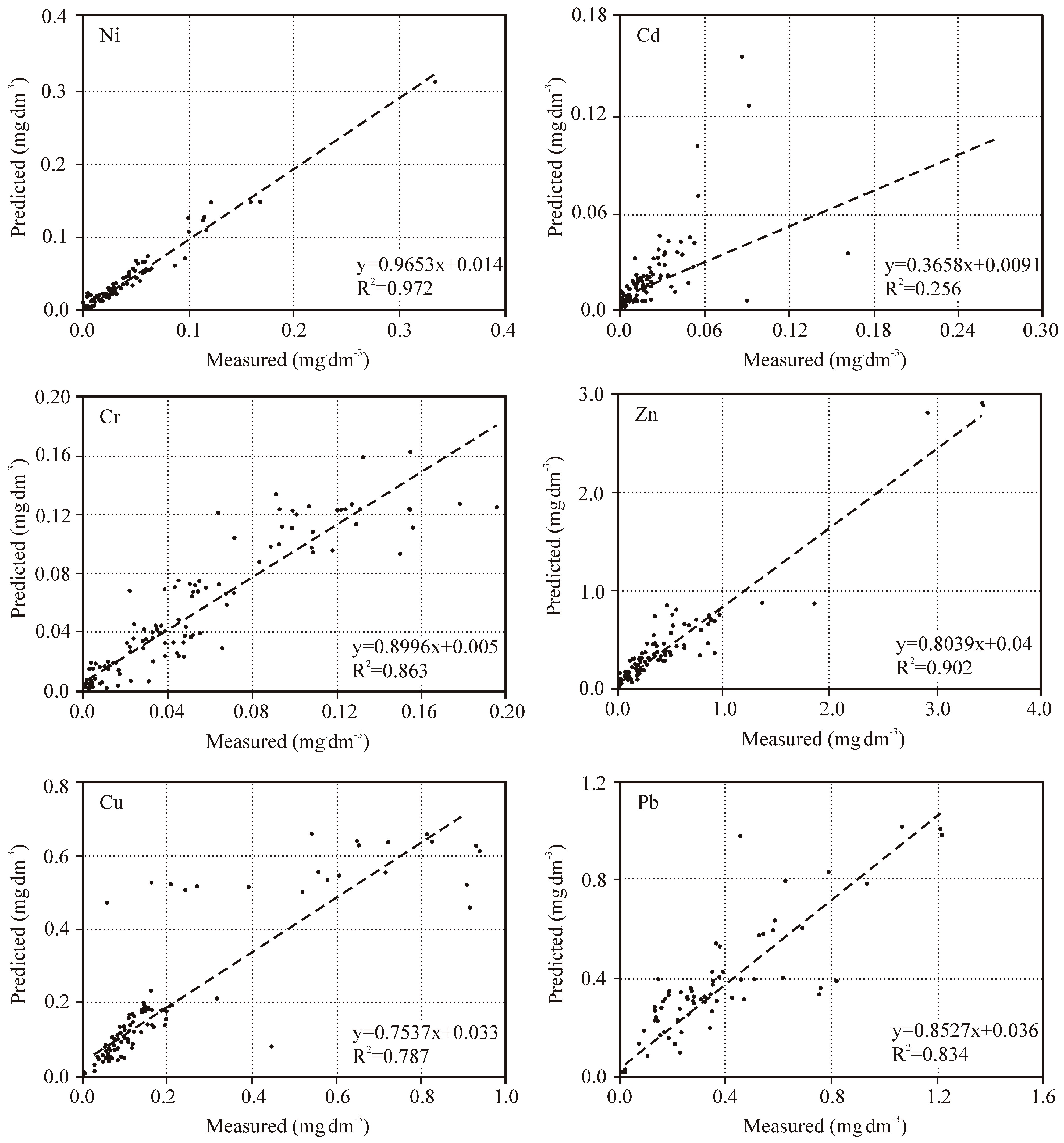
The parameters that characterise the structure of MLP models, namely number of neurons, activation functions in the hidden and output layers, are shown in Table 5. The values of measures of the model fit (R, MAE, RMSE) to experimental data are also given in the table. Based on the data from Table 5, it can be seen that for individual networks, a number of neurons in the hidden layer ranges from 28 to 35. Additionally, the analyses demonstrate that the number of neurons obtained for individual MLP models is not greater than that recommended [25]. The results show that for Ni and Zn, selected independent variables ensure satisfactory predictive capacities of HMC mathematical models—R2 > 0.90 (Figure 5). With regard to Cr and Pb, the fit of simulated values to the measured ones is also satisfactory (0.83 < R2 < 0.86). In addition, Figure 5 shows that the smallest scatter is found for concentrations lower than 0.08 mg∙dm−3 (Cr) and 0.4 mg∙dm−3 (Pb). With respect to Cu, good predictive abilities of the model are observed only up to the value of approx. 0.2 mg∙dm−3. The value of R2 = 0.256 for Cd shows poor fit between ANN predictions and measurements, especially for concentrations higher than 0.03 mg∙dm−3 (Figure 5).
The analyses indicate (Table 4) that the pattern of variation in HM concentrations for catchments with diversified land use is much more complex than in homogeneous catchments [46]. Additionally, in heterogeneous catchments, mechanisms affecting the quality and quantity of stormwater are far more complex. Consequently, taking into account simulation results, it is difficult to specify variables that decidedly determine HM concentrations. The concentrations of the analysed HM are affected to the greatest extent by the following values: G, P(10), Tme, wme and A (Table 3). It is necessary to conduct further investigations and select adequate computational models to identify key independent variables.
4. Conclusions
The computations performed for this study demonstrate it is possible to develop an ANN model to simulate variation in HM concentrations in stormwater and meltwater. The model is innovative because it attempts to simulate different mechanisms that affect HM concentrations. The use of a single mathematical model for that purpose has not been reported in the literature so far.
The computations show it is possible to simulate HM (Ni, Cd, Cu, Zn, Cr and Pb) concentrations in stormwater flowing from catchments with different types of land use. The ANN-based model employed to that end ensures satisfactory reliability. The results reported in the study demonstrate that HM concentrations in stormwater are affected by the physical and geographical characteristics of the catchment, and also by parameters describing atmospheric conditions and air quality. It is also shown that for heterogeneous catchments (as those investigated in the study), it is difficult to clearly specify key variables that decide the selected HM concentrations. To validate the ANN models developed for the study, it is necessary to conduct further field investigations.
The methodology proposed in the study is universal in character. The analysis of spatial data making up the catchment characteristics, which are retrieved from available databases (orthoimagery, base maps, digital elevation models—http://www.gis.kielce.eu/), measurements of atmospheric conditions and air quality, (alternatively available monitoring network data—https://en.tutiempo.net/climate/poland, http://smjp.kielce.pios.gov.pl/) and measurements of HM concentrations in stormwater can be combined. That provides a tool which can be applied to model HM concentrations in different scenarios. The ANN method employed in the study is commonly used in computational packages. As a result, the development of the model and the optimisation of its structure are not complex tasks (the parameters are automatically estimated by the programs, e.g., MATLAB), and such an approach will gain in popularity in engineering practice. The model can be applied to spatial development and planning. It can be used to seek optimal solutions in stormwater management intended to reduce the HM content flowing from the catchment.
Author Contributions
Conceptualisation, B.S. and J.G.; methodology, B.S. and Ł.B.; validation, Ł.B. and K.G.; formal analysis, B.S.; investigation, Ł.B. and J.G.; resources, K.G.; data curation, B.S.; writing—original draft preparation, B.S., Ł.B. and J.G.; writing—review and editing, J.G. and K.G.; visualisation, Ł.B.; supervision, B.S.; project administration, Ł.B.; funding acquisition, J.G.
Funding
This research was funded from the programme of the Minister of Science and Higher Education entitled “Regional Initiative of Excellence” in 2019–2022 project number 025/RID/2018/19 financing amount PLN 12,000,000”.
Conflicts of Interest
The funders had no role in the design of the study; in the collection, analyses, or interpretation of data; in the writing of the manuscript, or in the decision to publish the results.
References
- Ali, S.A.; Rodriguez, F.; Bonhomme, C.; Chebbo, G. Accounting for the Spatio-Temporal Variability of Pollutant Processes in Stormwater TSS Modeling Based on Stochastic Approaches. Water 2018, 10, 1773. [Google Scholar] [CrossRef]
- Tsai, L.Y.; Chen, C.F.; Fan, C.H.; Lin, J.Y. Using the HSPF and SWMM Models in a High Pervious Watershed and Estimating Their Parameter Sensitivity. Water 2017, 9, 780. [Google Scholar] [CrossRef]
- Cho, J.H.; Lee, J.H. Multiple Linear Regression Models for Predicting Nonpoint-Source Pollutant Discharge from a Highland Agricultural Region. Water 2018, 10, 1156. [Google Scholar] [CrossRef]
- Zawilski, M.; Sakson, G. Assessment of total suspended solid emission discharged via storm sewerage system from urban areas. Ochr. Srodowiska 2013, 35, 33–40. (In Polish) [Google Scholar]
- Yang, L.; Zhou, X.; Wang, Z.; Zhou, Y.; Cheng, S.; Xu, P.; Gao, X.; Nie, W.; Wang, X.; Wang, W. Airborne fine particulate pollution in Jinan, China: Concentrations, chemical compositions and influence on visibility impairment. Atmos. Environ. 2012, 55, 506–514. [Google Scholar] [CrossRef]
- Majewski, G.; Rogula-Kozłowska, W. The elemental composition and origin of fine ambient particles in the largest Polish conurbation: First results from the short-term winter campaign. Theor. Appl. Climatol. 2016, 125, 79–92. [Google Scholar] [CrossRef]
- Garcia, J.T.; Espin-Leal, P.; Vigueras-Rodriguez, A.; Carrillo, J.M.; Castillo, L.G. Synthetic pollutograph by prediction indices: An evaluation in several urban sub-catchnents. Sustainability 2018, 10, 2634. [Google Scholar] [CrossRef]
- Szeląg, B.; Barbusiński, K.; Studziński, J. Activated sludge process modelling using selected machine learning techniques. Desalin. Water Treat. 2018, 117, 78–87. [Google Scholar] [CrossRef]
- Bąk, Ł.; Szeląg, B.; Sałata, A.; Studziński, J. Modeling of Heavy Metal (Ni, Mn, Co, Zn, Cu, Pb, and Fe) and PAH Content in Stormwater Sediments Based on Weather and Physico-Geographical Characteristics of the Catchment-Data-Mining Approach. Water 2019, 11, 626. [Google Scholar] [CrossRef]
- May, D.B.; Sivakumar, M. Prediction of heavy metal concentrations in urban stormwater. Water Environ. J. 2009, 23, 247–254. [Google Scholar] [CrossRef]
- Pochwat, K. The use of artificial neural networks for analyzing the sensitivity of a retention tank. In Proceedings of the VI International Conference of Science and Technology INFRAEKO Modern Cities—E3S Web of Conferences 45, Krakow, Poland, 7–8 June 2018; p. 00066. [Google Scholar] [CrossRef]
- Mounce, S.R.; Shepherd, W.; Sailor, G.; Shucksmith, J.; Saul, A.J. Predicting combined sewer overflows chamber depth using artificial neural networks with rainfall radar data. Water Sci. Technol. 2014, 69, 1326–1333. [Google Scholar] [CrossRef]
- Singh, K.P.; Basant, A.; Malik, A.; Jain, G. Artificial neural network modeling of the river water quality—A case study. Ecol. Model. 2009, 220, 888–895. [Google Scholar] [CrossRef]
- Sarkar, A.; Pandey, P. River Water Quality Modelling Using Artificial Neural Network Technique. Aquat. Procedia 2015, 4, 1070–1077. [Google Scholar] [CrossRef]
- Bąk, Ł.; Górski, J.; Górska, K.; Szeląg, B. Suspended Solids and Heavy Metals Content of Selected Rainwater Waves in an Urban Catchment Area: A Case Study. Ochr. Srodowiska 2012, 34, 49–52. (In Polish) [Google Scholar]
- Górski, J.; Szeląg, B.; Bąk, Ł. The application of SWMM software for the evaluation of stormwater treatment plant operation. Woda Środ. Obsz. Wiej. 2016, 16, 17–35. (In Polish) [Google Scholar]
- PN-EN ISO 10523:2012. Water Quality. Determination pH Value; ISO: Geneva, Switzerland, 2012. (In Polish) [Google Scholar]
- PN-EN ISO 11885:2009. Determination of Selected Elements by Inductively Coupled Plasma Optical Emission Spectrometry (ICP-OES); ISO: Geneva, Switzerland, 2009. (In Polish) [Google Scholar]
- Arbeitsblatt DWA-A 118. Hydraulische Bemessung und Nachweis von Entwässerungssystemen; Deutsche Vereinigung für Wasserwirtschaft, Abwasser und Abfall: Hennef, Germany, 2006. [Google Scholar]
- Szeląg, B.; Kiczko, A.; Studziński, J.; Dąbek, L. Hydrodynamic and probabilistic modelling of storm overflow discharges. J. Hydroinform. 2018, 10, 1–11. [Google Scholar] [CrossRef]
- Box, G.E.P.; Cox, D.R. An analysis of transformations. J. R. Stat. Soc. B 1964, 26, 211–252. [Google Scholar] [CrossRef]
- Murphy, L.U. Quantifying Spatial and Temporal Deposition of Atmospheric Pollutants in Runoff from Different Pavement Types. Ph.D. Thesis, University of Canterbury Christchurch, Christchurch, New Zealand, 2015. [Google Scholar]
- Rutkowski, L. Artificial Intelligence Methods and Techniques; PWN: Warszawa, Poland, 2006. (In Polish) [Google Scholar]
- Hecht-Nielsen, R. Kolmogorov’s Mapping Neural Network Existence Theorem. In Proceedings of the IEEE First Annual International Conference on Neural Networks, San Diego, CA, USA, 21–24 June 1987. [Google Scholar]
- Demuth, H.; Beale, M. Neural Network Toolbox. For Use with MATLAB; The MathWorks: Natick, MA, USA, 2002. [Google Scholar]
- Fach, S.; Sitzenfrei, R.; Rauch, W. Assessing the relationship between water level and combined sewer overflow with computational fluid dynamics. In Proceedings of the 11th International Conference on Urban Drainage, Edinburgh, UK, 31 August–5 September 2008. [Google Scholar]
- Królikowski, A.; Garbarczyk, K.; Gwoździej-Mazur, J.; Butarewicz, A. Sediments Formed in Stormwater Sewer Facilities; Polish Academy of Sciences: Lublin, Poland, 2005. (In Polish) [Google Scholar]
- Górska, K.; Sikorski, M.; Górski, J. Occurrence of heavy metals in rain wastewater on example of urban catchment in Kielce. Ecol. Chem. Eng. A 2013, 20, 961–974. [Google Scholar] [CrossRef]
- Rogula-Kozłowska, W.; Majewski, G.; Czechowski, P.O. The size distribution and origin of elements bound to ambient particles: A case study of a Polish urban area. Environ. Monit. Assess. 2015, 187, 240. [Google Scholar] [CrossRef] [PubMed]
- Murphy, L.U.; Cochrane, T.A.; O’Sullivan, A. Build-up and wash-off dynamics of atmospherically derived Cu, Pb, Zn and TSS in stormwater runoff as a function of meteorological characteristics. Sci. Total Environ. 2015, 508, 206–213. [Google Scholar] [CrossRef] [PubMed]
- Hong, N.; Zhu, P.; Liu, A. Modelling heavy metals build-up on urban road surfaces for effective stormwater reuse strategy implementation. Environ. Pollut. 2017, 253, 821–828. [Google Scholar] [CrossRef] [PubMed]
- Djukić, A.; Lekić, B.; Rajaković-Ognjanović, V.; Veljović, D.; Vulić, T.; Djolić, M.; Naunovic, Z.; Despotović, J.; Prodanović, D. Further insight into the mechanism of heavy metals partitioning in stormwater runoff. J. Environ. Manag. 2016, 168, 104–110. [Google Scholar] [CrossRef] [PubMed]
- Sakson, G.; Zawilski, M.; Badowska, E.; Brzezińska, A. Stormwater pollution as the basis of choice the method of their management. J. Civ. Eng. Environ. Archit. 2014, 31, 253–264. [Google Scholar] [CrossRef]
- Lundy, L.; Ellis, J.B.; Revitt, D.M. Risk prioritisation of stormwater pollutant sources. Water Res. 2012, 46, 6589–6600. [Google Scholar] [CrossRef]
- Gasperi, J.; Kafi-Benyahia, M.; Lorgeoux, C.; Moilleron, R.; Gromaire, M.C.; Chebbo, G. Wastewater quality and pollutant loads in combined sewers during dry weather periods. Urban Water J. 2008, 5, 305–314. [Google Scholar] [CrossRef]
- Zgheib, S.; Moilleron, R.; Chebbo, G. Priority pollutants in urban stormwater: Part 1—Case of separate storm sewers. Water Res. 2012, 46, 6683–6692. [Google Scholar] [CrossRef]
- Gnecco, I.; Berretta, C.; Lanza, L.G.; La Barbera, P. Storm water pollution in the urban environment of Genoa, Italy. Atmos. Res. 2005, 77, 60–73. [Google Scholar] [CrossRef]
- Revitt, D.M.; Lundy, L.; Coulon, F.; Fairley, M. The sources, impact and management of car park runoff pollution: A review. J. Environ. Manag. 2014, 146, 552–567. [Google Scholar] [CrossRef] [Green Version]
- Gan, H.; Zhuo, M.; Li, D.; Zhou, Y. Quality characterization and impact assessment of highway runoff in urban and rural area of Guangzhou, China. Environ. Monit. Assess. 2008, 140, 147–159. [Google Scholar] [CrossRef]
- Brombach, H.; Fuchs, S. Datenpool Gemessener Verschmutzungskonzentrationen von Trocken—und Regenwetterabflüssen in Misch—und Trennkanalisationen; ATV-DVWK—Forschungsfonds, Projekt 1-01; GFA: Hennef, Germany, 2001. [Google Scholar]
- Charters, F.J.; Cochrane, T.A.; O’Sullivan, A. Untreated runoff quality from roof and road surfaces in a low intensity rainfall climate. Sci. Total Environ. 2016, 550, 265–272. [Google Scholar] [CrossRef]
- Valtanen, M.; Sillanpää, N.; Setälä, H. The Effects of Urbanization on Runoff Pollutant Concentrations, Loadings and Their Seasonal Patterns Under Cold Climate. Water Air Soil Pollut. 2014, 225, 1977. [Google Scholar] [CrossRef]
- Sternbeck, J.; Sjodin, A.; Andreasson, K. Metal emissions from road traffic and the influence of resuspension—Results from two tunnel studies. Atmos. Environ. 2002, 36, 4735–4744. [Google Scholar] [CrossRef]
- Bergbäck, B.; Johansson, K.; Mohlander, U. Urban Metal Flows—A Case Study of Stockholm. Review and Conclusions. Water Air Soil Pollut. Focus 2001, 1, 3–24. [Google Scholar] [CrossRef]
- Suresh, G.; Sutharsan, P.; Ramasamy, V.; Venkatachalapathy, R. Assessment of spatial distribution and potential ecological risk of the heavy metals in relation to granulometric contents of Veeranam lake sediments India. Ecotoxicol. Environ. Saf. 2012, 84, 117–124. [Google Scholar] [CrossRef]
- Gunawardena, J.; Ziyath, A.M.; Egodawatta, P.; Ayoko, G.A.; Goonetilleke, A. Sources and transport pathways of common heavy metals to urban road surfaces. Ecol. Eng. 2015, 77, 98–102. [Google Scholar] [CrossRef] [Green Version]
- Rocher, V.; Azimi, S.; Gasperi, J.; Beuvin, L.; Mulle, M.; Moilleron, R.; Chebbo, G. Hydrocarbons and metals in atmospheric deposition and roof runoff in central Paris. Water Air Soil Pollut. 2004, 159, 67–86. [Google Scholar] [CrossRef]
- Wicke, D.; Cochrane, T.A.; O’Sullivan, A.D. Atmospheric deposition and storm induced runoff of heavy metals from different impermeable urban surfaces. J. Environ. Monit. 2012, 14, 209–216. [Google Scholar] [CrossRef]
Figure 1.
Study area—(a) location in the city of Kielce; (b) IX Wieków Kielc stormwater treatment plant (SWTP) catchment; (c) Witosa SWTP catchment; and (d) Jesionowa SWTP catchment.
Figure 1.
Study area—(a) location in the city of Kielce; (b) IX Wieków Kielc stormwater treatment plant (SWTP) catchment; (c) Witosa SWTP catchment; and (d) Jesionowa SWTP catchment.

Figure 2.
Methodology of the development of multi-layer perceptron (MLP) model for predicting the selected pollutant concentrations in stormwater.
Figure 2.
Methodology of the development of multi-layer perceptron (MLP) model for predicting the selected pollutant concentrations in stormwater.

Figure 3.
Graphic interpretation of the trend function.

Figure 4.
The structure of the multi-layer perceptron artificial neural networks (ANN) model used for the study.
Figure 4.
The structure of the multi-layer perceptron artificial neural networks (ANN) model used for the study.
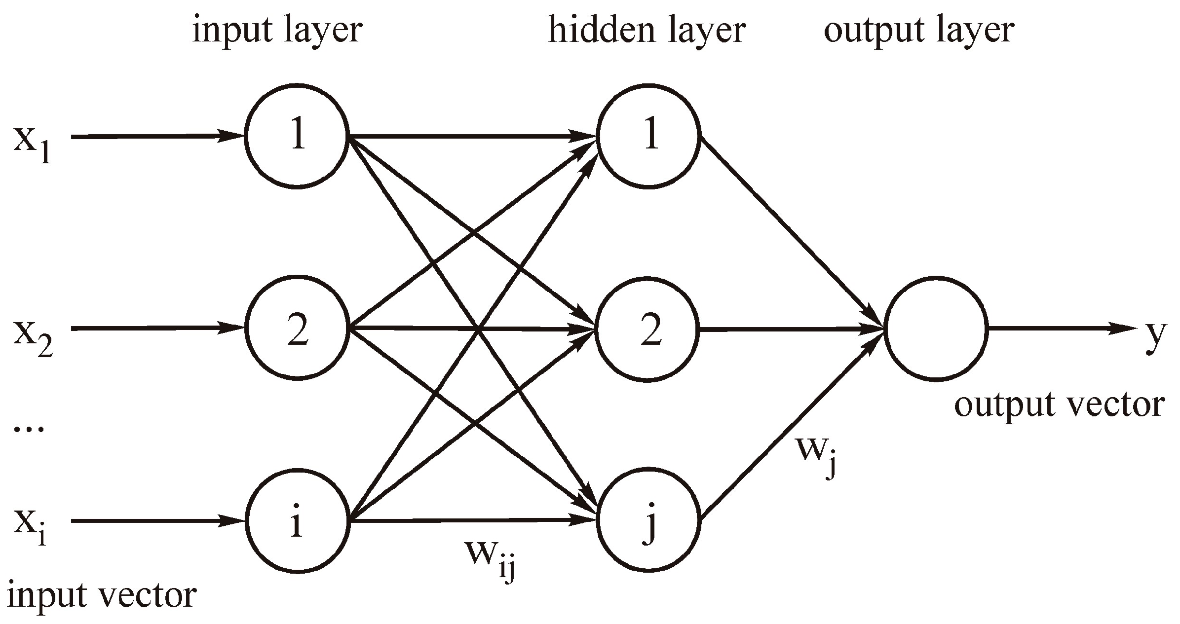
Figure 5.
Predicted versus observed HM concentrations in stormwater (validation step).

Table 1.
Land use characteristics.
| Catchment | Area A | Surface Type | ||||
|---|---|---|---|---|---|---|
| Roads | Roofs | Car Parks | Green Spaces | |||
| Asphalt | Gravel | |||||
| ha | % | |||||
| IX Wieków Kielc | 62 | 26.0 | – | 14.3 | 11.2 | 48.5 |
| Witosa | 83 | 8.5 | 1.6 | 9.4 | 6.4 | 74.1 |
| Jesionowa | 400 | 11.3 | 8.4 | 11.5 | 11.2 | 57.6 |
Table 2.
Summary statistics describing heavy metals concentrations in the analysed catchments.
| Years | Value (μg∙dm−3) | Cd | Cu | Cr | Ni | Pb | Zn |
|---|---|---|---|---|---|---|---|
| IX Wieków Kielc SWTP | |||||||
| 2009–2018 | Range | 0–162 | 0–1068 | 0–350 | 0–168 | 0–1405 | 0–3873 |
| Median | 20 | 128 | 70 | 45 | 411 | 430 | |
| Mean | 17 | 113 | 46 | 31 | 342 | 298 | |
| Witosa SWTP | |||||||
| 2015–2018 | Range | 1–766 | 3–959 | 3–319 | 2–341 | 1–343 | 45–3160 |
| Median | 37 | 358 | 70 | 38 | 55 | 663 | |
| Mean | 22 | 262 | 67 | 23 | 14 | 550 | |
| Jesionowa SWTP | |||||||
| 2016–2018 | Range | 4–649 | 5–660 | 14–2236 | 13–304 | 13–1115 | 319–5731 |
| Median | 16 | 128 | 177 | 74 | 138 | 1148 | |
| Mean | 7 | 99 | 117 | 80 | 101 | 842 | |
Table 3.
Matrix of Pearson correlation coefficients between selected heavy metal (HM) and catchment/atmosphere characteristics.
Table 3.
Matrix of Pearson correlation coefficients between selected heavy metal (HM) and catchment/atmosphere characteristics.
| Ni | Cu | Cr | Zn | Pb | Cd | Q | Ptot | P(10) | tr | tbd | G | |
|---|---|---|---|---|---|---|---|---|---|---|---|---|
| Ni | 1.00 | 0.57 * | 0.42 * | 0.61 * | 0.71 * | 0.72 * | −0.28 * | −0.43 * | −0.52 * | −0.11 * | −0.27 * | 0.49 * |
| Cu | 0.57 * | 1.00 | 0.81 * | 0.79 * | 0.58 * | 0.71 * | −0.24 * | −0.48 * | −0.53 * | −0.03 | −0.12 * | 0.40 * |
| Cr | 0.42 * | 0.81 * | 1.00 | 0.65 * | 0.57 * | 0.59 * | −0.06 | −0.26 * | −0.53 * | 0.06 | 0.00 | 0.17 * |
| Zn | 0.61 * | 0.79 * | 0.65 * | 1.00 | 0.65 * | 0.71 * | −0.22 * | −0.41 * | −0.45 * | 0.03 | −0.24 * | 0.39 * |
| Pb | 0.70 * | 0.57 * | 0.57 * | 0.66 * | 1.00 | 0.73 * | 0.02 | −0.17 * | −0.44 * | −0.11 * | −0.13 * | 0.24 * |
| Cd | 0.72 * | 0.71 * | 0.59 * | 0.71 * | 0.72 * | 1.00 | −0.26 * | −0.38 * | −0.49 * | −0.03 | −0.22 * | 0.39 * |
| wme | wvar | wgrad | Vime | Vivar | Vigrad | Tsn | Tf | Tme | Tvar | Tgrad | ts | |
| Ni | −0.71 * | −0.46 * | −0.15 * | 0.32 * | 0.51 * | 0.02 | 0.09 | −0.08 | −0.70 * | −0.24 * | −0.01 | 1.00 |
| Cu | −0.46 * | −0.28 * | −0.41 * | 0.39 * | 0.44 * | 0.27 * | 0.02 | 0.35 * | −0.60 * | 0.18 * | −0.16 * | −0.34 |
| Cr | −0.34 * | −0.31 * | −0.52 * | 0.44 * | 0.42 * | 0.29 * | −0.03 | 0.20 * | −0.46 * | 0.15 * | −0.19 * | −0.37 |
| Zn | −0.58 * | −0.29 * | −0.28 * | 0.42 * | 0.39 * | 0.12 * | −0.05 | 0.20 * | −0.70 * | 0.11 * | −0.10 * | −0.33 |
| Pb | −0.64 * | −0.45 * | −0.33 * | 0.47 * | 0.52 * | −0.03 | −0.05 | −0.16 * | −0.68 * | −0.28 * | 0.07 | −0.38 |
| Cd | −0.59 * | −0.52 * | −0.26 * | 0.35 * | 0.39 * | 0.21 * | 0.00 | 0.01 | −0.62 * | −0.07 | −0.19 * | −0.32 |
| Zi | A | |||||||||||
| RF | CP | GRD | GS | RD | ||||||||
| Ni | 0.43 * | 0.43 * | −0.26 * | −0.43 * | 0.43 * | −0.66 * | ||||||
| Cu | 0.13 * | 0.13 * | −0.49 * | −0.13 * | 0.14 * | −0.51 * | ||||||
| Cr | 0.28 * | 0.28 * | −0.33 * | −0.28 * | 0.29 * | −0.56 * | ||||||
| Zn | 0.19 * | 0.19 * | −0.45 * | −0.19 * | 0.19 * | −0.54 * | ||||||
| Pb | 0.71 * | 0.71 * | −0.12 * | −0.71 * | 0.71 * | −0.86 * | ||||||
| Cd | 0.34 * | 0.34 * | −0.31 * | −0.35 * | 0.34 * | −0.59 * | ||||||
* significant at p ≤ 0.05; RF, roofs; CP, car parks; GRD, gravel roads; GS, green spaces; RD, roads; Vi, visibility; T, air temperature; w, wind speed (me, median; var, variance; grad, gradient).
Table 4.
F and p values for the Fisher–Snedecor test.
| Ni | Cu | Cr | Zn | Pb | Cd | ||||||||||||
|---|---|---|---|---|---|---|---|---|---|---|---|---|---|---|---|---|---|
| Variable | F | p | Variable | F | p | Variable | F | p | Variable | F | p | Variable | F | p | Variable | F | p |
| G | 215 | <0.00001 | GRD | 68.2 | <0.00001 | A | 95.2 | <0.00001 | A | 49.4 | <0.00001 | RF | 215 | <0.00001 | A | 58.2 | <0.00001 |
| Tme | 92.6 | <0.00001 | RF | 68.2 | <0.00001 | CP | 56.7 | <0.00001 | CP | 24.8 | <0.00001 | CP | 215 | <0.00001 | G | 30.7 | <0.00001 |
| ts | 72.1 | <0.00001 | RD | 68.2 | <0.00001 | RF | 56.7 | <0.00001 | RF | 24.8 | <0.00001 | GS | 215 | <0.00001 | RD | 29.5 | <0.00001 |
| A | 63.9 | <0.00001 | CP | 68.2 | <0.00001 | RD | 56.7 | <0.00001 | RD | 24.8 | <0.00001 | RD | 215 | <0.00001 | CP | 29.5 | <0.00001 |
| CP | 46.7 | <0.00001 | GS | 68.2 | <0.00001 | GRD | 56.7 | <0.00001 | GS | 24.8 | <0.00001 | GRD | 215 | <0.00001 | RF | 29.5 | <0.00001 |
| RD | 46.7 | <0.00001 | A | 59.3 | <0.00001 | GS | 56.7 | <0.00001 | GRD | 24.8 | <0.00001 | A | 82.9 | <0.00001 | GS | 29.5 | <0.00001 |
| GRD | 46.7 | <0.00001 | wvar | 53.6 | <0.00001 | Tvar | 55.1 | <0.00001 | ts | 24.7 | <0.00001 | Vivar | 48.6 | <0.00001 | GRD | 29.5 | <0.00001 |
| RF | 46.7 | <0.00001 | Tvar | 53.4 | <0.00001 | ts | 52.1 | <0.00001 | wvar | 24.4 | <0.00001 | wvar | 41.7 | <0.00001 | ts | 26.3 | <0.00001 |
| GS | 46.7 | <0.00001 | ts | 46.2 | <0.00001 | Vime | 49.0 | <0.00001 | Tme | 16.6 | <0.00001 | ts | 34.3 | <0.00001 | wvar | 25.0 | <0.00001 |
| Vime | 41.1 | <0.00001 | G | 43.6 | <0.00001 | Tme | 37.6 | <0.00001 | Tvar | 16.5 | <0.00001 | Tme | 29.0 | <0.00001 | Tme | 21.1 | <0.00001 |
| wvar | 38.8 | <0.00001 | Tme | 38.6 | <0.00001 | Vivar | 27.7 | <0.00001 | wme | 14.7 | <0.00001 | wgrad | 24.5 | <0.00001 | tbd | 13.5 | <0.00001 |
| P(10) | 29.4 | <0.00001 | Q | 30.2 | <0.00001 | Tsn | 25.2 | <0.00001 | Vigrad | 12.8 | <0.00001 | tbd | 24.2 | <0.00001 | wme | 12.2 | <0.00001 |
| Vivar | 24.9 | <0.00001 | Tf | 22.3 | <0.00001 | Ptot | 21.6 | <0.00001 | Vime | 9.7 | <0.00001 | Vime | 21.4 | <0.00001 | Vime | 11.1 | <0.00001 |
| Ptot | 24.7 | <0.00001 | Ptot | 21.0 | <0.00001 | Q | 20.5 | 0.0001 | G | 9.3 | 0.0024 | Tf | 20.9 | <0.00001 | Ptot | 9.3 | <0.00001 |
| wme | 17.9 | <0.00001 | tr | 19.4 | <0.00001 | wgrad | 19.6 | <0.00001 | Ptot | 8.9 | <0.00001 | Ptot | 19.9 | <0.00001 | Tgrad | 9.1 | <0.00001 |
| Tsn | 17.4 | <0.00001 | Vigrad | 15.1 | <0.00001 | P(10) | 19.4 | <0.00001 | tr | 8.2 | <0.00001 | wme | 19.1 | <0.00001 | Tvar | 7.9 | <0.00001 |
| Tvar | 12.7 | <0.00001 | Tgrad | 13.2 | <0.00001 | Tf | 14.9 | <0.00001 | Tf | 7.9 | <0.00001 | Tvar | 18.9 | <0.00001 | Tf | 7.3 | <0.00001 |
| Tgrad | 11.7 | <0.00001 | P(10) | 9.9 | <0.00001 | Tgrad | 13.4 | <0.00001 | tbd | 6.2 | 0.0004 | Tsn | 15.1 | <0.00001 | Vivar | 6.7 | <0.00001 |
| Vigrad | 10.4 | <0.00001 | Vivar | 8.4 | <0.00001 | tr | 11.2 | <0.00001 | P(10) | 5.3 | 0.0001 | P(10) | 13.4 | <0.00001 | Vigrad | 6.4 | <0.00001 |
| tbd | 7.9 | <0.00001 | Vime | 5.6 | <0.00001 | G | 11.1 | 0.0010 | Tgrad | 3.2 | 0.0029 | Vigrad | 11.8 | <0.00001 | P(10) | 5.7 | <0.00001 |
| Tf | 6.8 | <0.00001 | wme | 0.32 | >0.05 | wvar | 9.0 | <0.00001 | Q | 0.26 | >0.05 | tr | 9.5 | <0.00001 | tr | 5.6 | <0.00001 |
| Q | 6.2 | <0.00001 | wgrad | 0.22 | >0.05 | tbd | 7.8 | <0.00001 | wgrad | 0.25 | >0.05 | Q | 5.2 | 0.0001 | Q | 4.2 | 0.0010 |
| tr | 3.7 | 0.0013 | tbd | 0.13 | >0.05 | wme | 6.3 | <0.00001 | Tsn | 0.18 | >0.05 | G | 0.31 | >0.05 | Tsn | 0.28 | >0.05 |
| wgrad | 0.17 | >0.005 | Tsn | 0.10 | >0.05 | Vigrad | 0.33 | >0.05 | Vivar | 0.11 | >0.05 | Tgrad | 0.28 | >0.05 | wgrad | 0.19 | >0.05 |
Table 5.
Parameters of ANN structure and model fit to experimental data.
| Heavy Metals | Number of Neurons | Activation Function | Training | Validation | |||||
|---|---|---|---|---|---|---|---|---|---|
| Hidden Layer | Output Layer | R | MAE | RMSE | R | MAE | RMSE | ||
| mg·dm−3 | mg·dm−3 | mg·dm−3 | mg·dm−3 | ||||||
| Ni | 28 | exp | tanh | 0.887 | 0.0093 | 0.0200 | 0.845 | 0.986 | 0.0043 |
| Cu | 30 | exp | tanh | 0.933 | 0.0374 | 0.0824 | 0.979 | 0.887 | 0.0457 |
| Cr | 32 | tanh | lin | 0.889 | 0.0130 | 0.0237 | 0.871 | 0.929 | 0.0113 |
| Zn | 35 | tanh | exp | 0.951 | 0.0931 | 0.1539 | 0.975 | 0.950 | 0.0871 |
| Pb | 33 | sigm | lin | 0.923 | 0.0489 | 0.1072 | 0.881 | 0.913 | 0.0557 |
| Cd | 35 | lin | tanh | 0.896 | 0.0044 | 0.0078 | 0.581 | 0.530 | 0.0083 |
R, correlation coefficient; MAE, mean absolute error; RMSE, root-mean-square error.
© 2019 by the authors. Licensee MDPI, Basel, Switzerland. This article is an open access article distributed under the terms and conditions of the Creative Commons Attribution (CC BY) license (http://creativecommons.org/licenses/by/4.0/).
Share and Cite
MDPI and ACS Style
Bąk, Ł.; Szeląg, B.; Górski, J.; Górska, K. The Impact of Catchment Characteristics and Weather Conditions on Heavy Metal Concentrations in Stormwater—Data Mining Approach. Appl. Sci. 2019, 9, 2210. https://doi.org/10.3390/app9112210
AMA Style
Bąk Ł, Szeląg B, Górski J, Górska K. The Impact of Catchment Characteristics and Weather Conditions on Heavy Metal Concentrations in Stormwater—Data Mining Approach. Applied Sciences. 2019; 9(11):2210. https://doi.org/10.3390/app9112210
Chicago/Turabian StyleBąk, Łukasz, Bartosz Szeląg, Jarosław Górski, and Katarzyna Górska. 2019. "The Impact of Catchment Characteristics and Weather Conditions on Heavy Metal Concentrations in Stormwater—Data Mining Approach" Applied Sciences 9, no. 11: 2210. https://doi.org/10.3390/app9112210
Note that from the first issue of 2016, this journal uses article numbers instead of page numbers. See further details here.